Article

Spatial Information Enhancement with Multi-Scale Feature Aggregation for Long-Range Object and Small Reflective Area Object Detection from Point Cloud

College of Electronic Science and Technology, National University of Defense Technology, Changsha 410073, China
*
Author to whom correspondence should be addressed.
These authors contributed equally to this work.
Remote Sens. 2024, 16(14), 2631; https://doi.org/10.3390/rs16142631
Submission received: 11 June 2024 / Revised: 13 July 2024 / Accepted: 16 July 2024 / Published: 18 July 2024

Abstract

:
Accurate and comprehensive 3D objects detection is important for perception systems in autonomous driving. Nevertheless, contemporary mainstream methods tend to perform more effectively on large objects in regions proximate to the LiDAR, leaving limited exploration of long-range objects and small objects. The divergent point pattern of LiDAR, which results in a reduction in point density as the distance increases, leads to a non-uniform point distribution that is ill-suited to discretized volumetric feature extraction. To address this challenge, we propose the Foreground Voxel Proposal (FVP) module, which effectively locates and generates voxels at the foreground of objects. The outputs are subsequently merged to mitigating the difference in point cloud density and completing the object shape. Furthermore, the susceptibility of small objects to occlusion results in the loss of feature space. To overcome this, we propose the Multi-Scale Feature Integration Network (MsFIN), which captures contextual information at different ranges. Subsequently, the outputs of these features are integrated through a cascade framework based on transformers in order to supplement the object features space. The extensive experimental results demonstrate that our network achieves remarkable results. Remarkably, our approach demonstrated an improvement of 8.56% AP on the SECOND baseline for the Car detection task at a distance of more than 20 m, and 9.38% AP on the Cyclist detection task.

1. Introduction

The development of autonomous driving technology has led to the burgeoning interest in 3D object detection. LiDAR has become one of the most popular sensors due to its ability to accurately capture 3D information in space with point clouds.
In contrast to 2D images, which utilize a pixel-based data structure, 3D detectors typically employ point clouds as input data, the inherent disorder and irregularity of which [1] bring challenges to the convolutional operation [2]. The majority of existing 3D detectors can be categorized into raw point cloud methods [1,3,4,5] and volumetric methods [6,7,8]. Prior methods directly consumed points and maintained the spatial information of the point clouds. For example, PointNet [1] and Part-A2 [5] employ multiple transform layers constructed with Multi-layer Perceptron (MLP) to aggregate the input points into aggregate point features, which are then output by a Feed Forward Network (FFN) to produce the k class classification scores. However, the raw point cloud is computationally expensive due to the 3D convolutions. In contrast to the aforementioned approaches, volumetric-based methods, such as [7,8], discretize the unstructured point clouds into a volumetric 3D grid of voxels, processing the voxel space similarly to the pixel space. However, the efficiency of the conversion from the point domain to the voxel domain exerts a strong influence on the detector potency.
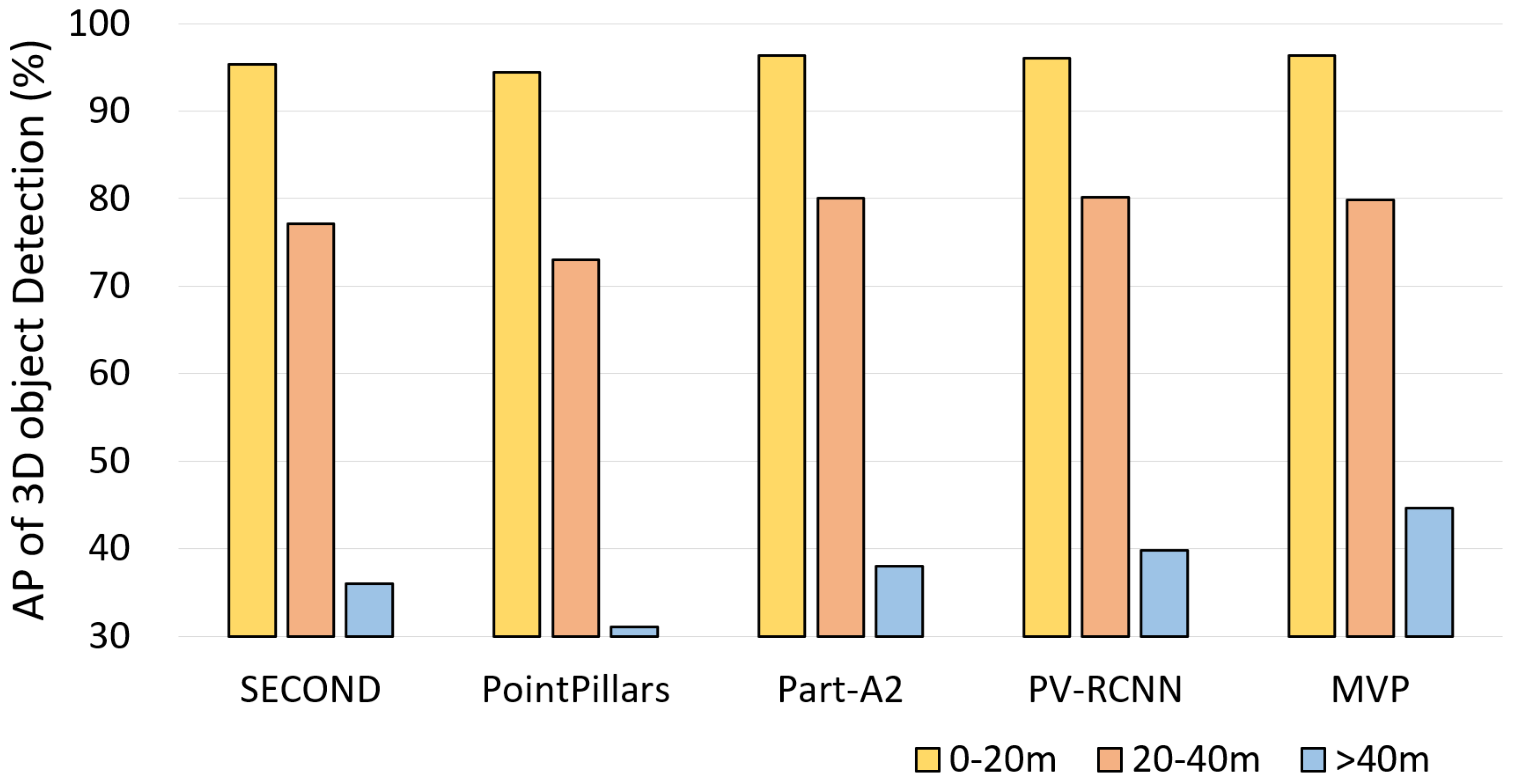
Although these approaches have demonstrated robust feature extraction capabilities on point clouds, they largely disregard the fact that LiDAR scanning angle changes result in the collected points naturally diverging as distance increases. Consequently, the number of points returned by closer distances is considerably greater than those returned at farther distances, resulting in a significant difference in point cloud density at different distance ranges from the LiDAR (as seen in Figure 1), which means point features extracted from sparse regions may generalize poorly to dense regions, and vice versa. As shown in Figure 2, most current methods ignore this density variation, resulting in a higher detection capability with Average Precision (AP) > 90% at near distance, far greater than than at far distance (AP of 30–45%).In autonomous driving, the system has more time and choices to make decisions when the effective detection range is greater and the detection categories are more comprehensive. For safety reasons, it is necessary to improve the detection accuracy of long-range objects.
Refs. [4,9] mitigate the issue of imbalance point density by Farthest Point Sampling (FPS), which extends the point set by selecting the points that are furthest away from the already selected point set to ensure that there is a uniform distribution of distances between the sampled points. By employing this methodology, the discrepancy in point density between dense and sparse regions can be mitigated by regulating the capacity of the point set. However, this approach entails a trade-off between resolution loss and point density. While it offers a more balanced spatial representation, it also results in a significant loss of spatial information.
In fact, even for long-range objects with a more decentralized distribution of points, strong representation capabilities still remain. Ref. [10] have demonstrated these representation capabilities by completing the sparse shape of an object to a dense shape with LiDAR points only. In addition, most networks rely heavily on the surface features, as the LiDAR beam has difficulty reaching the interior of the object, resulting in incomplete object coverage, especially for larger objects. It can be demonstrated that the unbalanced point density results in a learning bias towards the objects occupying the dense points in the detection (as seen in Appendix A). To overcome this limitation, we introduce the Foreground Voxel Proposal (FVP) module. Specifically, it aims firstly to voxelize the raw point cloud, which serves to overcome the disorder and irregularity inherent in the data. Subsequently, the FVP module employs the voxels of the foreground to generate proposal points that lie within the ground truth box, thereby enriching the internal information on objects and balancing the difference in point cloud density at different distances.
Once the voxels have been constructed, the next challenge lies in effectively extracting the features from the voxel space. However, the small objects within the autopilot scenario, such as pedestrians and cyclists, are more susceptible to occlusion due to their small reflective area. Meanwhile, the design of the convolution kernel limits the acquisition of global features, which is crucial for detecting small objects, such as cyclists and pedestrians. In order to enhance environmental coverage, it is essential to direct attention towards smaller objects, rather than solely focusing on larger ones. Current methods often overlook this crucial aspect [7,11,12,13]. Inspired by the accomplishments of vision transformer (ViT) [14], which regards the input features as patches and gains a global view by calculating the correlation between different patches, many approaches have been successful in capturing long-range information [12,15]. However the expending of the receptive fields imposes a burgeoning computational burden. To capture the long-range information while preserving local features, we propose a transformer-based cascade network named Multi-Scale Feature Integration Network (MsFIN). The key idea involves dividing the voxel space into multiple concentric 3D windows of varying sizes. By adopting self-attention with different rate of sampling, each size of window focuses on a different granularity of information with a controllable calculating burden. By cascading the concentric windows with cross-attention [14], the communication between windows is established. In order to assess the efficacy of our module, we conducted experiments on KITTI [16] dataset. Our results demonstrated that our module exhibited remarkable performance, particularly in the context of long-range and small objects. In summary, the main contributions of this paper are as follows:
  • A Foreground Voxel Proposal (FVP) module was designed to enhance point cloud density by proposing voxels at the foreground of sparse objects, thereby circumventing the bias that arises from an imbalanced point density. It improved the network’s detection capabilities of distant objects.
  • We present a Multi-scale Feature Integration Network (MsFIN) based on the cascading attention framework, which progressively incorporates contextual information at larger scales, supplementing the objects with surrounding voxel features. It improved the network’s detection capabilities of small-reflective-area objects.
  • We combine the FVP module with MsFIN and propose the Multi-scale Foreground Voxel Proposal (Ms-FVP) network, which balances the detection of long-range objects with that of small-reflective-area objects. We compare a variety of other models and demonstrate the effectiveness of our algorithm.
The structure of this paper is as follows: Section 2 reports the related research. Section 3 introduces the network structure and method in detail and Section 4 presents our work and experimental results and compares them with related methods to verify the effectiveness of our approach. Finally, Section 5 concludes the paper.

2. Related Work

This section reviews existing works on 3D object detection based on LiDAR point clouds. Then, we review the methods to counter the issues of non-uniform point density and occlusion in the 3D object detection of long-range objects and small-reflective-area objects. Finally, we introduce the transformer in 3D objection detection.

2.1. 3D Object Detection on Point Clouds

Detecting 3D objects from point clouds typically involves point-based detectors [4,17,18,19] and voxel-based detectors [5,6,8]. The point-based methods consume the point clouds directly and aggregate the features of an object from neighboring points. PointNet [1] extends the points’ features with a shared feed-forward network and uses the maximum function to aggregate the feature for the object. To better represent the local structure, PointNet++ [3] adopts a hierarchical structure, which can effectively extract local features in different areas based on different sensory field sizes. The voxel-based methods usually voxelize a point cloud into 3D grids with a specially designed local aggregation operators and then apply a Convolution Neural Network (CNN) to extract the features from a series of voxels. The local aggregation layer usually adopt the coordinates and features of points inside the grids as input, and outputs the combined result as a feature representation of the whole voxel. VoxelNet [6] utilizes PointNet [1,20] as the operator to aggregate features and then employ sparse 3D convolution to generate the detection outcome. However, due to the sparsity of the point cloud, a large number of convolutional computations are performed in a space with vacant feature, causing a computational burden. SECOND [8] mainly focuses on improving the performance of sparse convolutions to improve the computation efficiency. PointPillars [21] expends the scale in the height axis to format the voxel into a pillar, which allows the use of 2D CNNs to further increase efficiency. However, the loss of resolution in the height direction results in a reduction in detection accuracy. Pillarnet [20] further improves the inference accuracy of the pillar-based method by adding a neck network, while maintaining a high inference speed. In this paper, we employed the voxel-based approach Region Proposal Network (RPN) to ensure the efficiency.

2.2. Non-Uniform Density Point Cloud in 3D Detection

The distribution of 3D points across the distance range in a LiDAR point cloud for autonomous driving is inhomogeneous [22,23]. This is primarily due to the fixed scanning pattern of the LiDAR sensor and its limited beam resolution, which results in significant differences in point density between objects at different distances from the sensor. Ref. [24] put forward a density-adaptive sampling method that addresses the issue of point density while maintaining the point object representation. The method involves oversampling to balance the point density of the pre-mesh point cloud data, followed by empirical sampling of points from the balanced mesh. PDV [23] addresses this issue from an architectural standpoint by considering point density variations. The method employs a voxel point plasma to identify voxel features, thereby enabling their spatial localization. These features are then aggregated through a kernel density estimation-based density-aware Region of Interest (RoI) pooling module and self-attention mechanism. Refs. [10,25] viewed this problem as a complementary problem for a mutilated point cloud. The encoding–decoding module was designed to learn the complementation rule by using randomly sampled point clouds with complete point clouds as training data. ImVoteNet [26] combines images and point cloud for long-range object detection. Additional semantic information is provided to the object by using visible light features as a complement. SPG [27] adopts a hide-and-predict strategy, whereby a portion of the object’s points is deliberately concealed, while the remainder is left unaltered. This is achieved by monitoring the network’s generation of points on incomplete objects, thereby enhancing the network’s resilience. In this work, we address the issue of low accuracy in long-range object recognition due to a non-uniform point cloud distribution by upsampling the raw point cloud. However, to prevent the significant increase in computing burden that would result from upsampling the whole screen, we differentiate between the foreground and background of the point cloud. By supervising the network to upsampling solely based on the foreground points, we can efficiently enrich the point cloud without increasing the computational effort and improve the network robustness.

2.3. Small-Reflective-Area Object Detection in Point Cloud

In the context of 3D small-reflective-area object detection, the recognition accuracy is often negatively impacted by occlusion and adverse weather conditions, which result in the complete absence of object feature space. Refs. [28,29] improve the completeness performance of the point cloud feature space by utilizing adversarial networks for the purpose of complementing the feature space. Ref. [30] proposes a shape-completion method based on adversarial network inversion, which circumvents the necessity for pairwise real-data dependence by utilizing an adversarial network that has been pre-trained on the complete shape. This is achieved by searching for latent codes that will provide the complete shape that best reconstructs a given portion of the input. PillarNeXt [31] enhances network contextual connectivity by integrating multi-scale feature fusion, which aggregates features at different scales to provide more comprehensive information on small objects. MsSVT [32] explicitly divides attention head into multiple groups, with each group focusing on a specific range. This allows the system to gather both fine-grained and long-range information, which it then uses to gather supplementary contextual information from neighbouring groups to enrich the feature space of small objects. In this paper, we employ the large receptive field strategy. The objective of expanding the receptive field is to facilitate the acquisition of contextual information at different scales. The aggregation of multi-scale contextual information enables the acquisition of supplementary information for small-reflective-area objects.

2.4. Transformer-Based Network on Point Clouds

Since the Transform [14] model was proposed, it has made impressive achievements in various fields. Refs. [33,34,35,36,37] conducted an exploration of the application of a transformer in point clouds, demonstrating the potential of attentional mechanisms for capturing spatial dependencies. VoTr [12] employs the attention mechanism for the purpose of backbone construction. This is achieved through the utilization of self-attention for the extraction of inter-voxel features within voxels. CT3D [38] introduces a two-stage channel-wise transformer architecture for 3D object detection, which aggregates the features of all the points output by the encoder module into a global feature that represents the features of this proposal. In contrast, our method divides mixed windows and balanced sampling to achieve the more efficient fusion of multi-scale features within each attention layer. By specifically projecting different sizes of divided windows into query windows and applying cross-attention, not only does the voxel better understand global features, it can also learn the relationship between local and global features for multi-scale feature capture.

3. Method

In this section, we introduced our network for 3D object detection from point clouds. We begin by providing a detailed explanation of the Foreground Voxel Proposal module (Section 3.1), which generates points at the foreground space of the object in order to enhance the object’s features and achieve balanced point cloud density within the detection space. Subsequently, we delve into the specifics of the Multi-Scale Feature Integration Network (Section 3.2), which capture mixed-scale information for voxels. Lastly, we discuss the region proposal network and training targets (Section 3.3).
The pipeline of our network is present at Figure 3. The raw point cloud is firstly aggregated into voxels to counteracting disorder and irregularity. Then the foreground voxels are utilized for the proposing points by the Foreground Voxel Proposal module. The proposed points are then aggregated and merged to mitigate point density differences.
In order for the model to more effectively capture the long-range information, the Multi-Scale Feature Integration Network is adopted. Finally, we pass the multi-scale feature voxels to the spare convolution layers [8] for the further extraction of higher level features, which are then sent into the Region Proposal Network (RPN) to form the final result.

3.1. Foreground Voxel Proposal Module

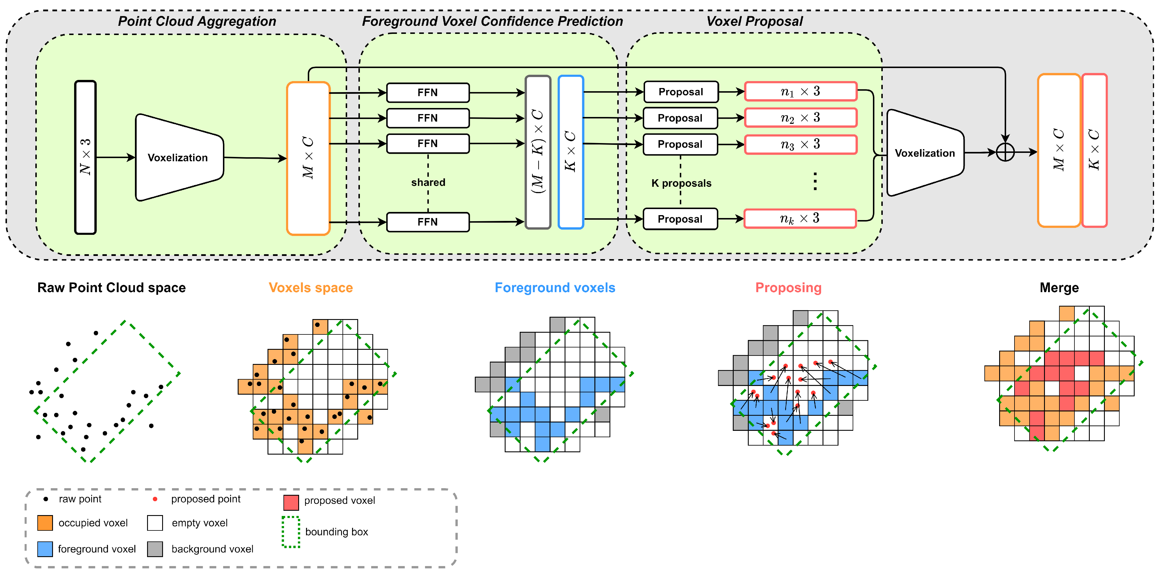
The overall architecture of FVP module is depicted in Figure 4. Initially, we divide the point space into grids and aggregate the point features in the same grid into voxels. For each voxel, the network predicts the probability of being a foreground voxel. Subsequently, the foreground voxels are required to proposal for the features of points located inside the object bounding box. Finally, we voxelize the proposal points and merge them with the raw voxels.

3.1.1. Point Cloud Aggregation

Since the typical LiDAR sensors can capture more than 100k points per frame on the streets [16,39,40], in order to avoid the high computation and memory requirements of directly consuming the raw points, we aggregate the raw points into voxels. Let c = { x m , y m , z m } be a voxel centroid with the arithmetic mean of all points in this voxel, and P = { p 1 , p 2 , . . . , p N } R 3 + F be the set of raw points of location x y z with F properties in the voxel. For each point p i within P , the point-wise enhancement is first performed:
p ˜ i = { f i x , f i y , f i z , F }
where f i x = { x i , Δ x i m } and Δ x i m is the distance to the voxel centroid at x dimension. Based on this, a simplified PointNet [1] is applied in each voxel with a multilayer perception (MLP) and a symmetry function to generate the voxel V:
V = MAX ( { MLP ( p ˜ i ) | i = 1 , . . . , M } )
where we use the MAX ( · ) as the symmetry function to make the model invariant to input permutation. Since it is common for the coordinates of points to be negative in LiDAR coordinate system, we also use LeakyReLU [41] instead of ReLU as the activation function to avoid the gradient vanishing.

3.1.2. Foreground Voxel Confidence Prediction

To generate the points within the foreground object bounding box, only the foreground voxels that contain the object information are considered to have the potential to make the points proposals. We regard all the voxels within the bounding box as the foreground voxels V f , and consider the remaining voxels as background. Each voxel undergoes processing through a shared FFN branch to encode features that contribute to determining the probability confidence P ˜ f . The probability confidence for each voxel is calculated as
P ˜ i f = σ ( FFN ( V i f ) )
where the σ is the Sigmoid function to normalizing the predicted probabilities, and V is the feature of the voxel. Restricting the foreground voxels from the proposal also keeps the number of generated points from being excessive, so as to avoid imposing a computational burden on the network.
To supervise P ˜ f , we use focal loss [42] to ensure a loss balance between foreground and background classes:
L V c l s = p f ( 1 p ˜ f ) γ log ( p ˜ f ) ( 1 p f ) ( p ˜ f ) γ log ( 1 p ˜ f )
where p f is the ground truth prediction and p f = 1 if the voxel belongs to the foreground else p f = 0 .

3.1.3. Voxel Proposal

Given a set of foreground voxels V f = { V i f | i = 1 , . . . , M } . We supervise the foreground voxels to generate the proposal points p ˜ p R 3 + P + F within the bounding box as
p ˜ i p = MLP ( [ V i f ; P ˜ i f ] )
Specifically, the proposal process is realized with an MLP network with fully connected layers, which is followed by batch normalization [43] and LeakyReLU. We additionally appended the probability confidence P f to generate the proposal points p p . The MLP takes the foreground voxel features V and the foreground probability confidence of the voxel to achieves the mapping R D R 3 + P + F , where the resulting vector consists of the proposal point coordinates offset Δ x i R 3 , P values for foreground probability confidence and the F-dimensional feature vector. We choose the K proposal points with the highest P f to generate the proposal voxels V p as described in Section 3.1.1, and merge them with the original voxels V to obtain the dense object representation.
We use Smooth-L1 loss for the regression of p ˜ p , which is calculated as
L V p r o p o s a l = 0.5 ( p p ˜ ) 2 if | p p ˜ | < 1 | p p ˜ | Otherwise
where p is the ground truth of the point feature. It is pertinent to mention that, given that the majority of the space in the foreground is devoid of points, we posit that the center of each empty voxel serves as the object of the regression.

3.2. Multi-Scale Feature Integration Network

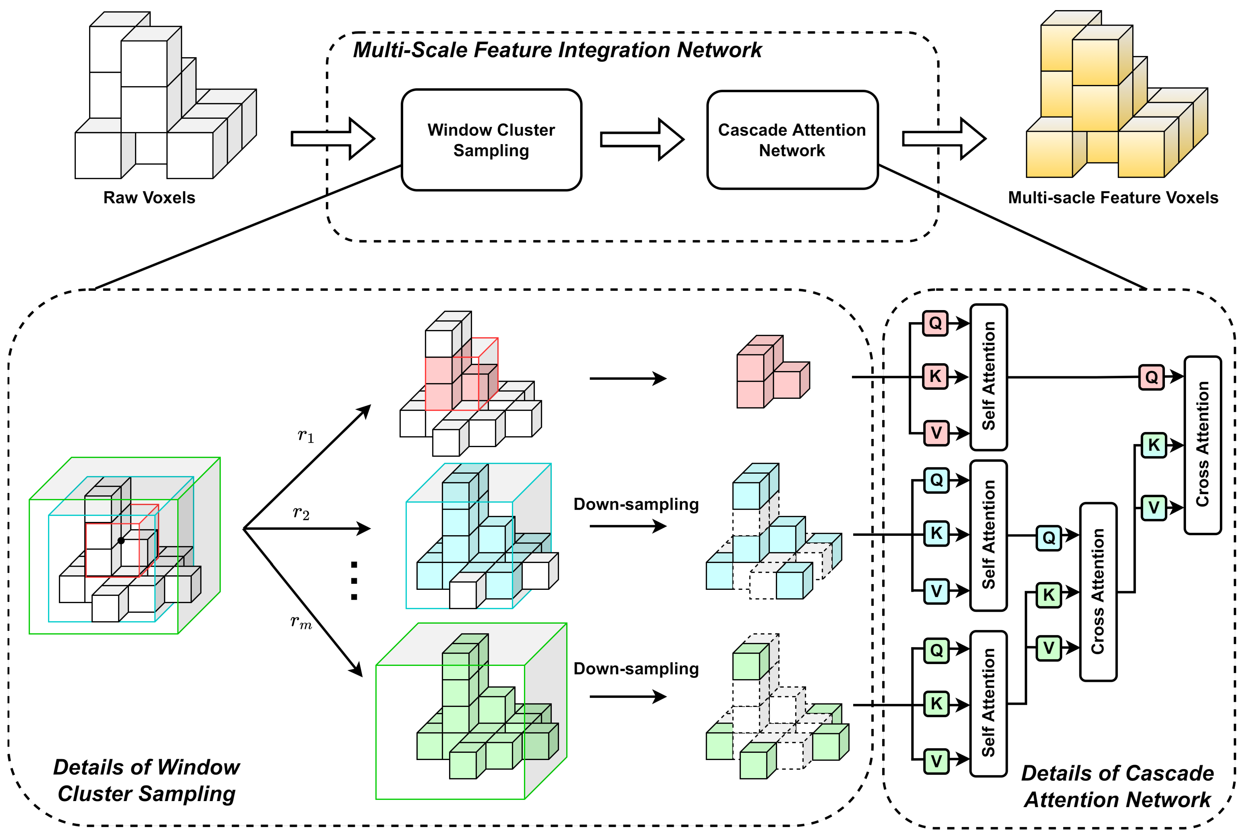
Global features can gather supplementary contextual information from neighboring areas, which is beneficial for a more comprehensive understanding of the detect space, particularly in the case of improving the detection performance on small-reflective-area objects such as cyclists and pedestrians. As shown in lower part of Figure 5, the detect space is initially divided into window clusters, each of which contains windows of different scales. Subsequently, the obtained windows are inputted into self-attention blocks to encode the visual word vector for each voxel. Lastly, we cascade the encoded windows with cross-attention to facilitate the extraction of mixed-scale information.

3.2.1. Window Cluster Sampling

We first divide the detect space into a series of non-overlapping 3D windows W 0 with size r 0 Z 3 as initial windows. The windows will be mostly empty or include few background points due to the sparsity of the point cloud. This sparsity is exploited by imposing a limit on the number of voxels inside the window; only windows with voxels greater than n 0 in W 0 are considered as valid windows. Consider { c j | c j = ( x , y , z ) j } j = 0 L as the center coordinates of W 0 , where L denotes the total numbers of valid initial windows. Then, centered on c , the space is divided into progressively larger windows of size r, where r = { r i | i = 1 , . . . , m } . Similarly, with operations as the initial windows, we save them only for windows with voxels greater than n i and adopt the FPS strategy to sample voxels within these windows to n i . We regard the set of windows with the same center c as a window cluster W j = { W 0 j , W 1 j , . . . W m j } j = 1 L , where W m is the window with size r m . By creating window clusters, we obtain a set of windows that contains the feature information of the same object at different scales. Also, the FPS step helps to reduce the memory consumption and balance the distribution of voxels within different window clusters from LiDAR.

3.2.2. Cascade Attention Network

We aggregate the features across stages to increase object appearance to more accurately and robustly detect distance. Initially, we compute word vectors for the voxels in the window with a self-attention block and represent them as
X = { x 0 , x 1 , . . . , x n }
where n is the total voxels in the window and x i R D is voxel feature with attentional weighting after passing through the self-attention mechanism. After that, we proceed with the establishment of the cascade network by project X j and X ˜ j + 1 to Q R N j × D , K R N j + 1 × D and V R N j + 1 × D with three learnable matrices, where X j is the visual words of the window with size r j and X ˜ j + 1 is the output of the previous attention stage. The output voxels of each stage are computed by
X ˜ j = σ Q j K j + 1 T k V j + 1
where σ ( · ) is the softmax function and k is a scaling factor to avoid gradient vanishing, with reference to [14]. By calculating the attention matrix separately for windows of different sizes r i , we can enrich the voxels with mixed-scale feature information.

3.2.3. Position Encoding

Position encoding has a crucial impact on the performance of a transformer-based network. We add relative Position Encoding to the self-attention module by using the absolute position and the relative position from the center of the window. The positional encoding for each voxel feature is calculated as
PE ( V j ) = FFN ( [ δ V j , c ] )
where c is the center coordinates of a window and δ V j = x V j c is the relative position of voxel V from center of the window which it belongs. By simply concatenating the voxel feature and corresponding Position Encoding, we finished the position embedding for each voxel.

3.2.4. Sparse Accelerator

For the significant memory and computational burden in voxel transformer, a method must be applied. We use the sparse accelerator to counter the sparsity of the voxel, fullfill the positioning of center voxel and the collect voxels inside the windows. Sparse accelerator mapping of a sparse coordinate space to a dense voxels index is achieved by building a hash table as discussed in [12]. The hash table contains two rows, preserving values and keys separately, where values keep the features of voxels and keys are related to the voxel coordinates, and each voxel corresponds to a unique key. For the query coordinates, the accelerator decides whether the corresponding voxel exists based on the return of the queried hash value. For example, we gather each feasible coordinate inside the window when establishing the window cluster. These coordinates are then converted to the query keys by a hash function, and only the values corresponding to valid keys are retained. We followed the hash function discussed in [12] as
b x m a x y m a x z m a x + x y m a x z m a x + y z m a x + z
where x m a x , y m a x , z m a x represent the maximum range of detect space, and b , x , y , z denote the batch index and the coordinates of a voxel. The hash function use the linear probing scheme to resolve the collisions in the hash table. With the parallel capability of CUDA, coordinates queries can be processed in parallel, which further accelerates the voxel searching process. By leveraging the per-built hash table, we efficiently build the window clusters for the following steps.

3.3. Region Proposal Network

We use the region proposal network similar to SECOND [8], which is composed of several convolution layers with each followed with BatchNormal and ReLU layers. Finally, the 1 × 1 convolutions are applied to generate classification vector, regression offsets and direction vector. For the regression, we encode the box as
Δ x = x g t x p d , Δ y = y g t y p d , Δ z = z g t z p d Δ l = log l g t l p , Δ w = log w g t w p , Δ h = log h g t h p Δ θ = s i n ( θ g t θ p )
where x g t and x p are, respectively, the ground truth and prediction and d = ( w p ) 2 + ( l p ) 2 is the distance between. The box regression loss is
L r e g = b ( x , y , z , l , w , h , θ ) SmoothL 1 ( Δ b )
We use the focal loss as the object classification loss:
L c l s = α a ( 1 p a ) γ log p a
where p a is the class probability of the anchor and α is the weight of each class. We set α = 0.25 and γ = 2 as described in [8].

4. Experiments

We evaluate our algorithms by comparing them with existing algorithms on the KITTI dataset, using both performance metrics and a qualitative perspective. Furthermore, the detection capabilities of the algorithms are evaluated for objects at varying distances. Finally, the contribution of each module to the network is analyzed.

4.1. Implementation Details

The size of the voxel used for the voxelization was (0.075 m, 0.075 m, 0.2 m). In the MsFIN, each window cluster contains two scales of windows with sizes of (2 m, 2 m, 2 m) and (5 m, 5 m, 5 m), and the voxel centroid coordinates wrapped by the window are counted as an asset of the window. For the windows in the window cluster, the number of preset voxels N i is 32 with the smaller window and 512 with the larger one.
Our model is trained end-to-end for 80 epochs using AdamW optimizer [44]. The learning rate is initially set to 1 × 10 4 and increases to 1 × 10 3 during the first 40% of the epochs and decreases to 1 × 10 5 in the last 20% of the epochs. We also augment the dataset by dumping a 1% percentile of all points’ heights to avoid the impact of ground points on detection. All experiments are conducted using Python 3.8 on one machine with 8 RTX 3090 GPUs and 2.8 GHz AMD EPYC 7402.

4.2. Result on KITTI

In this section, a comparison is made between the ability to detect objects at different distances in the KITTI dataset, as well as the ability to detect objects at different levels of difficulty, with other existing methods.

4.2.1. Dataset Setups

All experiments use KITTI object detection benchmark dataset [16]. The KITTI dataset contains 3712 training samples, 3769 validation samples [7] and 7518 test samples. Only the points within the field of view are retained because these are the only regions that have been labeled.
The evaluation metric we used is the Average Precision (AP) for 3D detection task and Bird’s Eye View (BEV) detection task, with three difficulty levels based on the number of points occupied by the object and the degree of truncation: Easy, Moderate, and Hard. We also report the results on the validation set at different distance ranges.

4.2.2. Main Results

Since point clouds of different densities can introduce data density imbalance problems, as discussed before, the capability of FPV for objects at different distance ranges was first evaluated. We split the validation set into three copies based on the distance of the object, containing three different distances, i.e., 0–20 m, 20–40 m and over 40 m. As shown in the fifth and the last columns in Table 1, the mean Average Precision (mAP) results of all three distances in our work outperforms previous methods, with 0.83% on the 3D detection task and 0.8% on the BEV detection task. For rear objects less than 20 m away, the performance obtained is comparable to the most effective algorithms, while as the distance increases, our method shows better performance, leading SIENet by 0.73% AP in the BEV detection task at distances of 0–20 m, and by 2.15% AP at distances over 40 m. A similar trend can be also observed in the 3D detection task, with our method leading SIENet by 0.87% AP at distances of 20–40 m and by 1.89% AP in comparison to MVP at distances exceeding 40 m. It is noted that our method has a slightly lower performance in the under 20 m range. Given that the AP baseline for close objects is sufficiently high (>95%), and the ability to detect mid-range and long-range objects in autonomous driving is of greater importance for the safety during driving, we consider such an inconsistency to be acceptable. These results provide compelling evidence of the efficacy of our methodology.
Additionally, Table 2 presents the detection result on the Car, Pedestrian and Cyclist categories. Our network outperforms other models at the Hard and Moderate level, which are mainly composed of sparse point set objects and obscured objects. We outperformed VoxelRCNN on 3D Car detection by 1.04% and 0.31% on Moderate AP and Hard AP, respectively. Moreover, our model exhibits excellent performance in the detection of of small objects, achieving 6.86% AP over VoxelNet [6] in the Pedestrian category at the Hard level and a striking 26.6% AP in the Cyclist category at the Hard level. To compare it with the second best result, our Pedestrian result outperformed VoxelRCNN by 1.47% on Hard AP and 0.18% on Moderate AP. The same trend is also shown in the detection of cyclists, as shown in the ninth and tenth columns.

4.2.3. Visualization

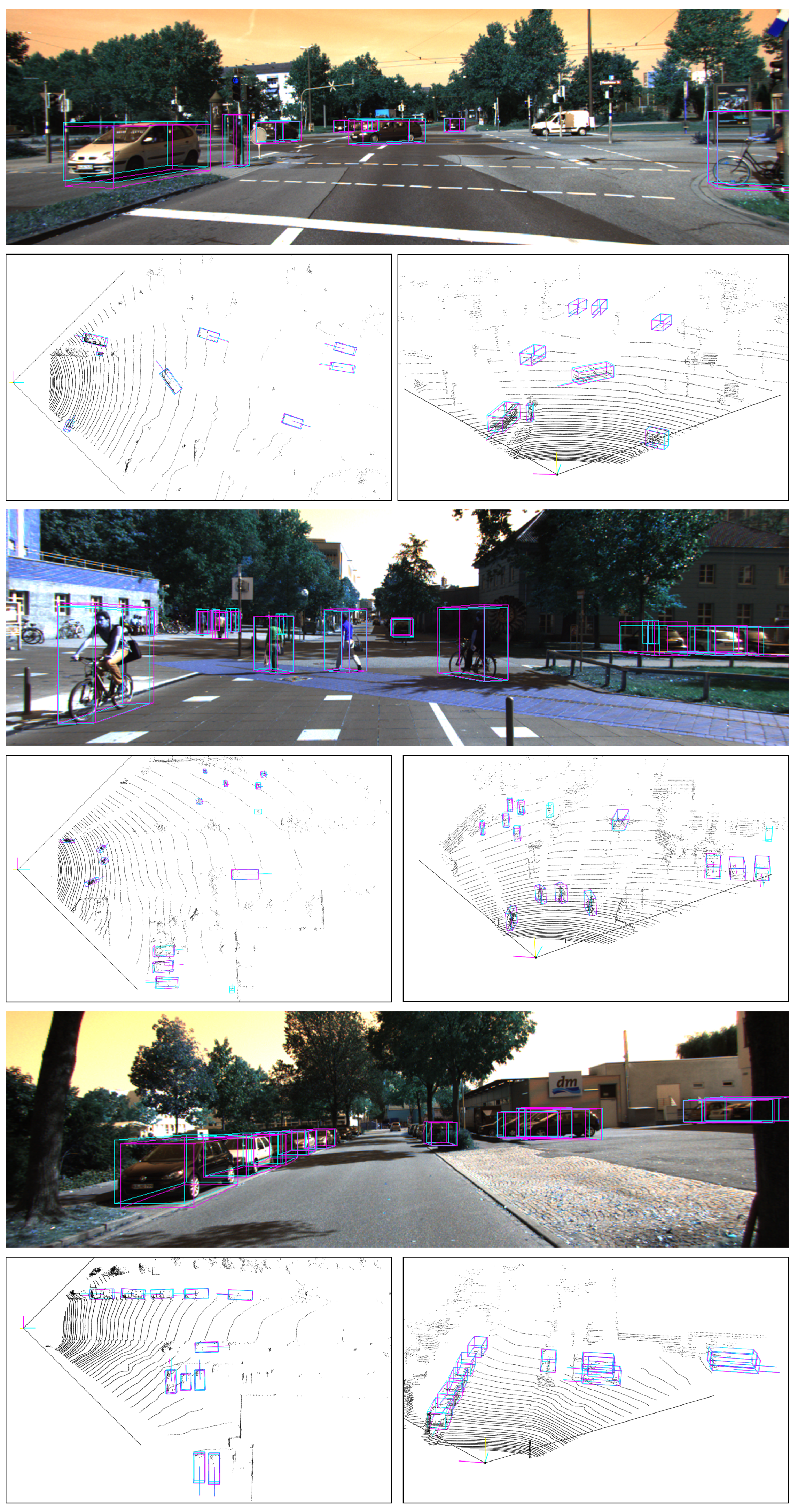
Qualitative Results. The results on the KITTI dataset demonstrate the excellent detection capability of our method, especially for long-range objects and small objects. We also present the qualitative results in Figure 6. Notably, our method demonstrates the capability of accurately detecting an object at a distance of more than 50 m with an extremely sparse distribution of points, as shown in the upper portion of Figure 6. This remarkable capability proves the effectiveness of our work in balancing the bias of point clouds, as well as complementing the shape of the object. The result also provides a comprehensive detection of multiple-sized objects, as shown in the middle part of Figure 6, which includes pedestrian, cyclist and car objects at different distances. The crowd was still well detected despite the long distance (left front of the LiDAR). Nevertheless, when confronted with exceedingly sparse and isolated objects, the limited local features with the isolated location make it difficult for the window of the Cascade Attention Network to capture more global information for it. The lower section of Figure 6 exhibits the excellent detection in scenarios involving a large number of objects in close proximity to one another.
Visualization of Proposed Voxels. To gain a better understanding of the Foreground Voxel Proposal module, we visualize the intermediate results produced during the proposing of foreground voxels. The number of points on a object at long distances is typically fewer and more dispersed. As depicted in the upper part of Figure 7, the FVP module generates voxels at both the surface edge and inner of the object, which effectively guides the network to regress on objects with insufficient features. The lower part of Figure 7 presents the street screen prediction results with and without the FVP module, which shows two common misjudgments in the case of point sparsity, i.e., positional errors and missed detection. The introduction of the FVP module has been shown to significantly enhance the detection ability in the case of long-range objects and those with occluded parts. This observation serves to illustrate the capacity of the FVP module to generate voxels, thereby enhancing the object information and reducing the bias impact of imbalanced point density, which in turn leads to an increased probability of identifying the object.
Visualization of Cascade Attention. In order to analyze the impact of a larger receptive field for small-reflective-area object recognition, we visualized the results of the Cascade Attention Network. As depicted in Figure 8a, the loss of feature information in objects due to occlusion is significant, which leads to less attention given to the object area due to the inability for the local receptive field to extract more valid information, resulting in missed detection. After switching to a larger sensory field (Figure 8b), we found that the network could still assign higher weights to the object region. At the same time, more additional information is captured by the network due to the expanded receptive field. Finally we cascade the results from the different receptive fields as described in Section 3.2, and find that the network increased the weight to the objects in (a). This is due to the fact that a larger receptive field allows for the acquisition of more feature information from nearby objects, which in turn enables the detection of objects that are not feature-rich with greater accuracy. Figure 8d,e illustrate that even in cases where the feature set is incomplete, our Multi-Scale Feature Integration Network can be utilized to improve the efficacy of identifying objects that are devoid of features.

4.3. Ablation Studies

In this section, the efficacy of the proposed method was evaluated through ablation experiments, which involved the validating of the components and parameter settings.

4.3.1. Effect of Key Components

We examine the impact of the crucial components, namely the Voxel Proposal, Cascade Attention Network, Window Cluster Sampling and Position Encoding. The network was incrementally augmented with these modules in order to facilitate the analysis of each structure, as depicted in Table 3.
Voxel Proposal. First, the Voxel Proposal strategy is assessed. As shown in the first row, we used a base model that is only composed of the point cloud aggregate followed by the convolution layers and detection head. To investigate the impact of our Voxel Proposal strategy, we insert our module before the convolution layers of the base model and combine the proposed voxels with the origins. As shown in the first and second row of Table 3, by limiting the number of participating voxels to those in the foreground and suppressing the proposing results of those in the background through the confidence of foreground prediction, we significantly improved the performance in all three categories, with the most significant AP improvement being in the car objects: from 78.46% to 80.98%.
Cascade Attention Network. We explore the effects of the Cascade Attention Network. We employed a base windows-based attention [48] and use the single size window of ( 5 , 5 , 5 ) with the random sampling. As a comparison, we use a two level cascade network to apply attention to the same window. As shown in the second and third row of Table 3, the AP performance improved from 56.01% to 56.31% for the Pedestrian category and from 70.01% to 70.86% for the Cyclist category, suggesting that the cascade attention mechanism has the ability to be made aware of different aspects of the features, and collects additional feature information from the neighborhood to complement the object features.
Window Cluster Sampling. The effect of Window Cluster Sampling is presented in the third and fourth row of Table 3. The use of different sampling rates for different window sizes ensures that the network can efficiently acquire both fine-grained local features and long-range information simultaneously. The adoption of the Window Cluster Sampling significantly increases the AP by 1.04% and 2.48% in the Pedestrian and Cyclist categories, respectively. Furthermore, the data also indicates an improvement in the detection of the Car category from 83.53% AP to 85.10% AP.
Position Encoding. The effect of Position Encoding presented in the final two rows of Table 3 demonstrates that incorporating Position Encoding improves the performance compared to the base model without a Position Encoding strategy. The results indicate a improvement on all three categories.

4.3.2. Impact of Foreground Voxel Confidence Prediction Settings

We further explored the impact of different prediction settings on network performance. As illustrated in the first and second row of Table 3, the network exhibits enhanced performance when foreground prediction constraints are imposed, in comparison to the scenario where confidence is not constrained. To illustrate the effect of the confidence prediction strategy, we change the setting of the confidence threshold, and present the results of the comparison in Table 4. As shown in the first three rows, the exclusion of background voxels from all proposing voxels resulted in an improvement in the detection performance. In our test, the best detection performance could be obtained by using 0.5 as the threshold. After that, as the threshold rises, the performance starts to decrease and eventually fluctuates within an interval. To explain this, we further analyzed the proposed quality. As shown in the second column, which presents the best proposal out of all proposals, we see that foreground voxels are more likely to be proposed in the foreground space and the background voxels are more inclined to introduce unwanted noise due to the lack of structural information. It is important to note that as the threshold increases, the number of voxels generated begins to decline and eventually becomes insufficient to have a significant impact on the prediction results.

4.3.3. Impact of Window Cluster Sampling Settings

We examine the impact of varying window sizes on performance. As shown in Table 5, we used a combination of three different window sizes. As seen in the first row in the table, the application of two relatively larger-sized windows was the least effective on all three categories. We attribute these results to the larger windows introducing a loss of local information during the sampling step. Furthermore, we used a small and a large window for pairing as shown in the final two rows. Significant performance gains were achieved after replacing a larger window with a small window, especially for the small-reflective-area objects. It is notable that the performance gain from further replacement with the larger window is not significant, as the size of (5 m, 5 m, 5 m) is already able to accommodate the majority of the categories in our test.

5. Conclusions

In this paper, we propose a LiDAR-based 3D object detection network that focus on improving the detection performance of long-range objects and small-reflective-area objects in an urban autonomous driving scenario. In the case of long-range objects with an extremely sparse point distribution, the proposed detector employs a foreground Voxel Proposal strategy that enables the generation of voxels within foreground objects. This mitigates the imbalance of point cloud density bias and enhances spatial information. Furthermore, for small objects that are prone to feature loss due to occlusion, a cascade attention structure is proposed to capture voxels with both local and long-range information, effectively gathering supplementary contextual information from neighbouring voxels. The efficacy of our method has been demonstrated through extensive experimental evaluations. We evaluated our method using KITTI and it outperforms the previous work in the detection tasks of long-range objects and small-reflective-area objects. However, a slight lower detection accuracy occurred with near objects compared to the current state-of-the-art algorithms. We speculate that this is due to the fact that we did not improve the detection head to a significant extent, as we focused our efforts on the processing of the point cloud of the long-range objects and the small-reflective-area objects. In future work, we will investigate the potential for enhancing the detection process to achieve further improvements in performance.

Author Contributions

Conceptualization, H.L.; methodology, H.L.; software, H.L. and H.T.; validation, H.L., H.T. and Q.D.; formal analysis, H.L.; investigation, H.L., Q.D. and S.X.; resources, H.L., S.X. and J.Z.; data curation, H.L. and Q.D.; writing—original draft preparation, H.L.; writing—review and editing, H.L., H.T., Q.D., S.X. and J.Z.; visualization, H.L.; supervision, H.T. and Q.D.; project administration, H.T.; funding acquisition, H.T. All authors have read and agreed to the published version of the manuscript.

Funding

The APC was funded by Research Project on Laser object Feature Extraction and Recognition.

Data Availability Statement

The KITTI dataset was obtained from https://www.cvlibs.net/datasets/kitti, accessed on 25 September 2022.

Conflicts of Interest

The authors declare no conflict of interest.

Appendix A

We assume that the non-uniform distribution of the point cloud introduces a bias as a factor in the lower detection accuracy of long-range objects. To test our hypothesis, we randomly sampled point clouds at near distances and then trained the processed dataset with PointPillars [21]. The result in Figure A1 exhibits an improved performance on long-range objects.
Figure A1. mAP for PointPillars [21] detector evaluated on KITTI validation dataset. The result on PointPillars trained on KITTI point clouds with and without 50% random sampling at a distance range of (0, 10) m are represented with a red bar and yellow bar, separately.
Remotesensing 16 02631 g0a1

References

  1. Qi, C.R.; Su, H.; Mo, K.; Guibas, L.J. Pointnet: Deep learning on point sets for 3d classification and segmentation. In Proceedings of the IEEE Conference on Computer Vision and Pattern Recognition, Honolulu, HI, USA, 21–26 July 2017; pp. 652–660. [Google Scholar]
  2. He, K.; Zhang, X.; Ren, S.; Sun, J. Deep residual learning for image recognition. In Proceedings of the IEEE Conference on Computer Vision and Pattern Recognition, Las Vegas, NA, USA, 27–30 June 2016; pp. 770–778. [Google Scholar]
  3. Qi, C.R.; Yi, L.; Su, H.; Guibas, L.J. Pointnet++: Deep hierarchical feature learning on point sets in a metric space. Adv. Neural Inf. Process. Syst. 2017, 30. [Google Scholar]
  4. Shi, S.; Wang, X.; Li, H. Pointrcnn: 3d object proposal generation and detection from point cloud. In Proceedings of the IEEE/CVF Conference on Computer Vision and Pattern Recognition, Long Beach, CA, USA, 15–20 June 2019; pp. 770–779. [Google Scholar]
  5. Shi, S.; Wang, Z.; Shi, J.; Wang, X.; Li, H. From points to parts: 3d object detection from point cloud with part-aware and part-aggregation network. IEEE Trans. Pattern Anal. Mach. Intell. 2020, 43, 2647–2664. [Google Scholar] [CrossRef] [PubMed]
  6. Zhou, Y.; Tuzel, O. Voxelnet: End-to-end learning for point cloud based 3d object detection. In Proceedings of the IEEE Conference on Computer Vision and Pattern Recognition, Salt Lake City, UT, USA, 18–28 June 2018; pp. 4490–4499. [Google Scholar]
  7. Deng, J.; Shi, S.; Li, P.; Zhou, W.; Zhang, Y.; Li, H. Voxel r-cnn: Towards high performance voxel-based 3d object detection. In Proceedings of the AAAI Conference on Artificial Intelligence, Virtual, 2–9 February 2021; Volume 35, pp. 1201–1209. [Google Scholar]
  8. Yan, Y.; Mao, Y.; Li, B. Second: Sparsely embedded convolutional detection. Sensors 2018, 18, 3337. [Google Scholar] [CrossRef] [PubMed]
  9. Shi, S.; Guo, C.; Jiang, L.; Wang, Z.; Shi, J.; Wang, X.; Li, H. Pv-rcnn: Point-voxel feature set abstraction for 3d object detection. In Proceedings of the IEEE/CVF Conference on Computer Vision and Pattern Recognition, Washington, DC, USA, 14–19 June 2020; pp. 10529–10538. [Google Scholar]
  10. Li, Z.; Yao, Y.; Quan, Z.; Xie, J.; Yang, W. Spatial information enhancement network for 3D object detection from point cloud. Pattern Recognit. 2022, 128, 108684. [Google Scholar] [CrossRef]
  11. Mao, J.; Niu, M.; Bai, H.; Liang, X.; Xu, H.; Xu, C. Pyramid r-cnn: Towards better performance and adaptability for 3d object detection. In Proceedings of the IEEE/CVF International Conference on Computer Vision, Virtual, 19–25 June 2021; pp. 2723–2732. [Google Scholar]
  12. Mao, J.; Xue, Y.; Niu, M.; Bai, H.; Feng, J.; Liang, X.; Xu, H.; Xu, C. Voxel transformer for 3d object detection. In Proceedings of the IEEE/CVF International Conference on Computer Vision, Montreal, QC, Canada, 10–17 October 2021; pp. 3164–3173. [Google Scholar]
  13. Zheng, W.; Tang, W.; Jiang, L.; Fu, C.W. SE-SSD: Self-ensembling single-stage object detector from point cloud. In Proceedings of the IEEE/CVF Conference on Computer Vision and Pattern Recognition, Virtual, 19–25 June 2021; pp. 14494–14503. [Google Scholar]
  14. Vaswani, A.; Shazeer, N.; Parmar, N.; Uszkoreit, J.; Jones, L.; Gomez, A.N.; Kaiser, Ł.; Polosukhin, I. Attention is all you need. Adv. Neural Inf. Process. Syst. 2017, 30. [Google Scholar]
  15. Fan, L.; Pang, Z.; Zhang, T.; Wang, Y.X.; Zhao, H.; Wang, F.; Wang, N.; Zhang, Z. Embracing single stride 3d object detector with sparse transformer. In Proceedings of the IEEE/CVF Conference on Computer Vision and Pattern Recognition, New Orleans, LA, USA, 19–24 June 2022; pp. 8458–8468. [Google Scholar]
  16. Geiger, A.; Lenz, P.; Stiller, C.; Urtasun, R. Vision meets robotics: The kitti dataset. Int. J. Robot. Res. 2013, 32, 1231–1237. [Google Scholar] [CrossRef]
  17. Qi, C.R.; Litany, O.; He, K.; Guibas, L.J. Deep hough voting for 3d object detection in point clouds. In Proceedings of the IEEE/CVF International Conference on Computer Vision, Seoul, Republic of Korea, 27 October–2 November 2019; pp. 9277–9286. [Google Scholar]
  18. Yang, Z.; Sun, Y.; Liu, S.; Shen, X.; Jia, J. Std: Sparse-to-dense 3d object detector for point cloud. In Proceedings of the IEEE/CVF International Conference on Computer Vision, Seoul, Republic of Korea, 27 October–2 November 2019; pp. 1951–1960. [Google Scholar]
  19. Yang, Z.; Sun, Y.; Liu, S.; Jia, J. 3dssd: Point-based 3d single stage object detector. In Proceedings of the IEEE/CVF Conference on Computer Vision and Pattern Recognition, Washington, DC, USA, 14–19 June 2020; pp. 11040–11048. [Google Scholar]
  20. Shi, G.; Li, R.; Ma, C. Pillarnet: Real-time and high-performance pillar-based 3d object detection. In Proceedings of the European Conference on Computer Vision, Tel Aviv, Israel, 24–28 October 2022; Springer: Berlin/Heidelberg, Germany, 2022; pp. 35–52. [Google Scholar]
  21. Lang, A.H.; Vora, S.; Caesar, H.; Zhou, L.; Yang, J.; Beijbom, O. Pointpillars: Fast encoders for object detection from point clouds. In Proceedings of the IEEE/CVF Conference on Computer Vision and Pattern Recognition, Long Beach, CA, USA, 16–17 June 2019; pp. 12697–12705. [Google Scholar]
  22. Corral-Soto, E.R.; Bingbing, L. Understanding strengths and weaknesses of complementary sensor modalities in early fusion for object detection. In Proceedings of the 2020 IEEE Intelligent Vehicles Symposium (IV), Las Vegas, NV, USA, 19 October–13 November 2020; IEEE: Piscataway, NJ, USA, 2020; pp. 1785–1792. [Google Scholar]
  23. Hu, J.S.; Kuai, T.; Waslander, S.L. Point density-aware voxels for lidar 3d object detection. In Proceedings of the IEEE/CVF Conference on Computer Vision and Pattern Recognition, New Orleans, LA, USA, 19–24 June 2022; pp. 8469–8478. [Google Scholar]
  24. Arief, H.A.; Arief, M.; Bhat, M.; Indahl, U.G.; Tveite, H.; Zhao, D. Density-Adaptive Sampling for Heterogeneous Point Cloud Object Segmentation in Autonomous Vehicle Applications. In Proceedings of the CVPR Workshops, Long Beach, CA, USA, 16–17 June 2019; pp. 26–33. [Google Scholar]
  25. Yuan, W.; Khot, T.; Held, D.; Mertz, C.; Hebert, M. Pcn: Point completion network. In Proceedings of the 2018 International Conference on 3D Vision (3DV), Piscataway, NJ, USA, 5–8 September 2018; pp. 728–737. [Google Scholar]
  26. Qi, C.R.; Chen, X.; Litany, O.; Guibas, L.J. Imvotenet: Boosting 3d object detection in point clouds with image votes. In Proceedings of the IEEE/CVF Conference on Computer Vision and Pattern Recognition, Virtual, 14–19 June 2020; pp. 4404–4413. [Google Scholar]
  27. Xu, Q.; Zhou, Y.; Wang, W.; Qi, C.R.; Anguelov, D. Spg: Unsupervised domain adaptation for 3d object detection via semantic point generation. In Proceedings of the IEEE/CVF International Conference on Computer Vision, Virtual, 19–25 June 2021; pp. 15446–15456. [Google Scholar]
  28. Tsai, D.; Berrio, J.S.; Shan, M.; Nebot, E.; Worrall, S. Viewer-centred surface completion for unsupervised domain adaptation in 3D object detection. In Proceedings of the 2023 IEEE International Conference on Robotics and Automation (ICRA), IEEE, London, UK, 29 May–2 June 2023; pp. 9346–9353. [Google Scholar]
  29. Chen, X.; Chen, B.; Mitra, N.J. Unpaired point cloud completion on real scans using adversarial training. arXiv 2019, arXiv:1904.00069. [Google Scholar]
  30. Zhang, J.; Chen, X.; Cai, Z.; Pan, L.; Zhao, H.; Yi, S.; Yeo, C.K.; Dai, B.; Loy, C.C. Unsupervised 3d shape completion through gan inversion. In Proceedings of the IEEE/CVF Conference on Computer Vision and Pattern Recognition, Virtual, 19–25 June 2021; pp. 1768–1777. [Google Scholar]
  31. Li, J.; Luo, C.; Yang, X. PillarNeXt: Rethinking network designs for 3D object detection in LiDAR point clouds. In Proceedings of the IEEE/CVF Conference on Computer Vision and Pattern Recognition, Vancouver, Canada, 18–22 June 2023; pp. 17567–17576. [Google Scholar]
  32. Dong, S.; Ding, L.; Wang, H.; Xu, T.; Xu, X.; Wang, J.; Bian, Z.; Wang, Y.; Li, J. Mssvt: Mixed-scale sparse voxel transformer for 3d object detection on point clouds. Adv. Neural Inf. Process. Syst. 2022, 35, 11615–11628. [Google Scholar]
  33. Guo, M.H.; Cai, J.X.; Liu, Z.N.; Mu, T.J.; Martin, R.R.; Hu, S.M. Pct: Point cloud transformer. Comput. Vis. Media 2021, 7, 187–199. [Google Scholar] [CrossRef]
  34. Zhao, H.; Jiang, L.; Jia, J.; Torr, P.H.; Koltun, V. Point transformer. In Proceedings of the IEEE/CVF International Conference on Computer Vision, Virtual, 19–25 June 2021; pp. 16259–16268. [Google Scholar]
  35. He, C.; Li, R.; Li, S.; Zhang, L. Voxel set transformer: A set-to-set approach to 3d object detection from point clouds. In Proceedings of the IEEE/CVF Conference on Computer Vision and Pattern Recognition, New Orleans, LA, USA, 19–24 June 2022; pp. 8417–8427. [Google Scholar]
  36. Zhang, C.; Wan, H.; Liu, S.; Shen, X.; Wu, Z. Pvt: Point-voxel transformer for 3d deep learning. arXiv 2021, arXiv:2108.06076. [Google Scholar]
  37. Park, C.; Jeong, Y.; Cho, M.; Park, J. Fast point transformer. In Proceedings of the IEEE/CVF Conference on Computer Vision and Pattern Recognition, New Orleans, LA, USA, 19–24 June 2022; pp. 16949–16958. [Google Scholar]
  38. Sheng, H.; Cai, S.; Liu, Y.; Deng, B.; Huang, J.; Hua, X.S.; Zhao, M.J. Improving 3d object detection with channel-wise transformer. In Proceedings of the IEEE/CVF International Conference on Computer Vision, Virtual, 19–25 June 2021; pp. 2743–2752. [Google Scholar]
  39. Sun, P.; Kretzschmar, H.; Dotiwalla, X.; Chouard, A.; Patnaik, V.; Tsui, P.; Guo, J.; Zhou, Y.; Chai, Y.; Caine, B.; et al. Scalability in perception for autonomous driving: Waymo open dataset. In Proceedings of the IEEE/CVF Conference on Computer Vision and Pattern Recognition, Virtual, 14–19 June 2020; pp. 2446–2454. [Google Scholar]
  40. Chang, M.F.; Lambert, J.; Sangkloy, P.; Singh, J.; Bak, S.; Hartnett, A.; Wang, D.; Carr, P.; Lucey, S.; Ramanan, D.; et al. Argoverse: 3d tracking and forecasting with rich maps. In Proceedings of the IEEE/CVF Conference on Computer Vision and Pattern Recognition, Long Beach, CA, USA, 16–17 June 2019; pp. 8748–8757. [Google Scholar]
  41. Xu, J.; Li, Z.; Du, B.; Zhang, M.; Liu, J. Reluplex made more practical: Leaky ReLU. In Proceedings of the 2020 IEEE Symposium on Computers and Communications (ISCC), Piscataway, NJ, USA, 7–10 July 2020; pp. 1–7. [Google Scholar]
  42. Lin, T.Y.; Goyal, P.; Girshick, R.; He, K.; Dollár, P. Focal loss for dense object detection. In Proceedings of the IEEE International Conference on Computer Vision, Honolulu, HI, USA, 21–26 July 2017; pp. 2980–2988. [Google Scholar]
  43. Ioffe, S.; Szegedy, C. Batch normalization: Accelerating deep network training by reducing internal covariate shift. In Proceedings of the International Conference on Machine Learning, Lille, France, 6–11 July 2015; pp. 448–456. [Google Scholar]
  44. Loshchilov, I.; Hutter, F. Decoupled weight decay regularization. arXiv 2017, arXiv:1711.05101. [Google Scholar]
  45. Shi, S.; Wang, Z.; Wang, X.; Li, H. Part-a2 net: 3d part-aware and aggregation neural network for object detection from point cloud. arXiv 2019, arXiv:1907.03670. [Google Scholar]
  46. Yin, T.; Zhou, X.; Krähenbühl, P. Multimodal virtual point 3d detection. Adv. Neural Inf. Process. Syst. 2021, 34, 16494–16507. [Google Scholar]
  47. Shi, S.; Jiang, L.; Deng, J.; Wang, Z.; Guo, C.; Shi, J.; Wang, X.; Li, H. PV-RCNN++: Point-voxel feature set abstraction with local vector representation for 3D object detection. Int. J. Comput. Vis. 2023, 131, 531–551. [Google Scholar] [CrossRef]
  48. Liu, Z.; Lin, Y.; Cao, Y.; Hu, H.; Wei, Y.; Zhang, Z.; Lin, S.; Guo, B. Swin transformer: Hierarchical vision transformer using shifted windows. In Proceedings of the IEEE/CVF International Conference on Computer Vision, Virtual, 19–25 June 2021; pp. 10012–10022. [Google Scholar]
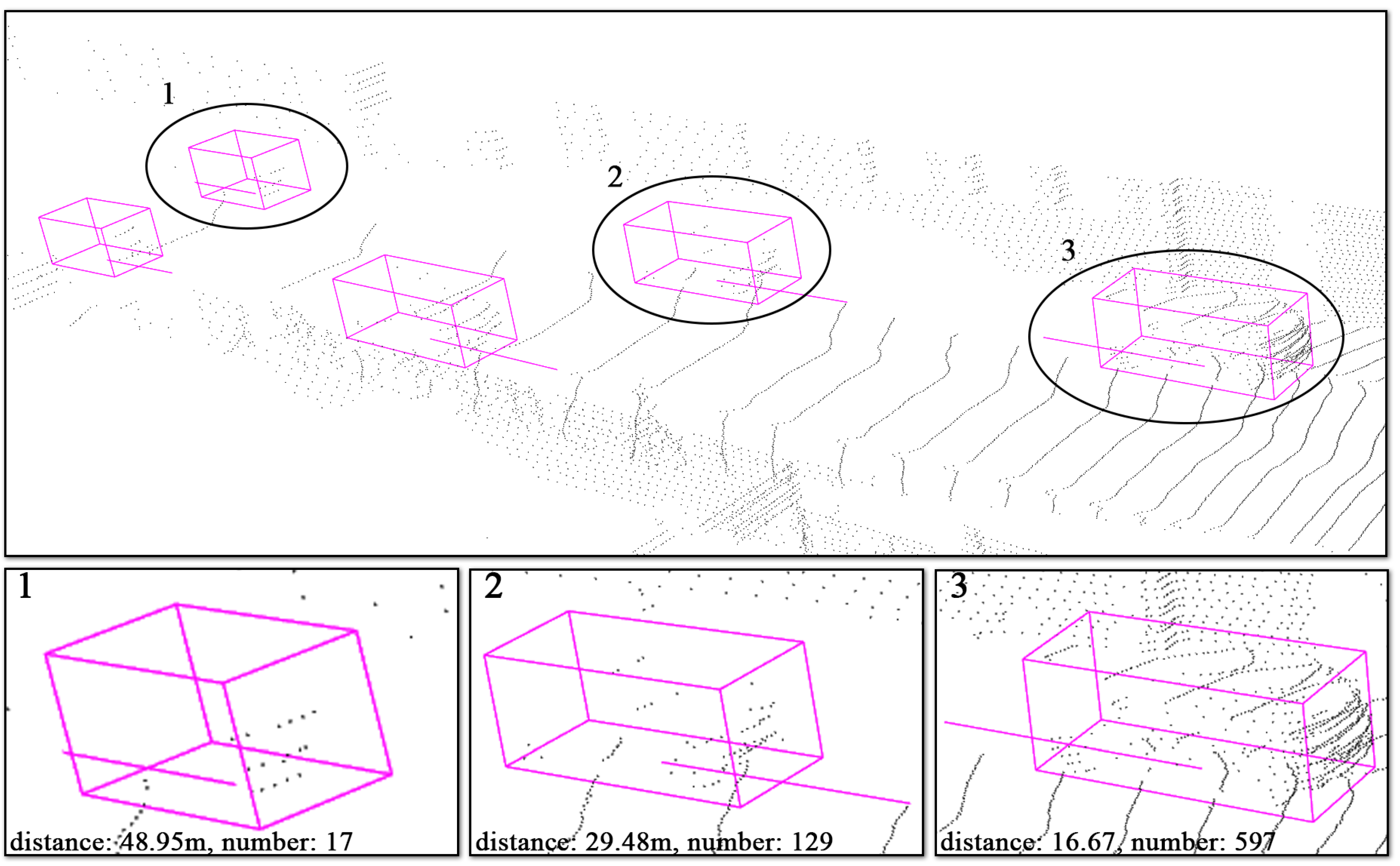
Figure 1. Illustration of the imbalanced point density on the KITTI dataset. (Top): The raw point cloud with green 3D bounding boxes. (Bottom): The zoomed-in display of three different distance objects with distance and point number information labeled. We use the line point from the center to direction to specify the direction the object is heading.
Remotesensing 16 02631 g001
Figure 2. Detection performance of state-of-the-art methods at different distances.
Remotesensing 16 02631 g002
Figure 3. The overarching architecture of our detection framework.
Remotesensing 16 02631 g003
Figure 4. Illustration of FVP module. In order to provide a more comprehensive illustration of the processing flow, we simplify the three-dimensional space into two dimensions by compressing along the height direction.
Remotesensing 16 02631 g004
Figure 5. Pipeline of Multi-Scale Feature Integration Network.
Remotesensing 16 02631 g005
Figure 6. Qualitative result of FVPNet on KITTI dataset. We use the line point from the center to specify the direction in which the object is heading.
Remotesensing 16 02631 g006
Figure 7. The visualization of proposed voxel. (a) The RGB image of detect screen and object. (b) The voxel space of object. (c) The proposed voxels (Green) merged with origin voxels (Black). (d,e) The predicted result with and without the Foreground Voxel Proposal module. where the Blue boxes and Purple boxes are the generated and predicted objects.
Remotesensing 16 02631 g007
Figure 8. The visualization of cascade attention effect. (a) The attention map of the small-size window. (b) The attention map of the large-size window. (c) The attention map of the cascade network. (d,e) are the predicted result.
Remotesensing 16 02631 g008
Table 1. Average Precision (%) comparison of Car detection task at different distance ranges. The result is reported on the R40. We mark the best result in bold and second best in underline.
Method   3D Detection   BEV Detection
0–20 m20–40 m>40 mMean0–20 m20–40 m>40 mMean
SECOND [8]95.3277.0835.9769.4696.1488.8954.3179.78
PointPillars [21]94.1576.4131.2467.2695.6387.6650.6677.98
Part-A2 [45]96.3080.0338.0171.4596.6988.5954.6579.97
PV-RCNN [9]96.0280.1039.8071.9796.3688.8555.4780.23
MVP [46]96.3579.8344.6273.6096.9689.2258.8381.67
SIENet [10]96.2382.7844.5974.5396.6789.7060.3782.25
Ms-FVP (Ours)95.9383.6546.5175.3696.2290.4362.5283.05
Table 2. Average Precision (%) comparison on KITTI val and test set. We use R40 recall for the AP in the Car, Pedestrian and Cyclist categories. The best result is marked in bold and the second best is marked with an underline.
MethodParam Validation Test
  3D Car (IoU = 0.7)  3D Ped. (IoU = 0.5)  3D Cyc. (IoU = 0.5)  3D Car (IoU = 0.7)
EasyMod.HardEasyMod.HardEasyMod.HardEasyMod.Hard
VoxelNet [6]6.4 M81.9765.4662.8557.8653.4248.8767.1747.6545.1177.4765.1157.73
SECOND [8]5.3 M86.4677.2874.6561.6356.2752.6080.1062.6959.7184.6575.9668.71
PointPillars [5]4.8 M88.6178.6277.2256.5552.9847.7380.5967.1653.1182.5874.3168.99
3DSSD [19]2.8 M88.5578.4577.3058.1854.3249.5686.2570.4965.3288.3679.5774.55
VoTr-SS [36]4.8 M87.8678.2776.93------88.3679.5774.55
VoxelSet [35]3.1 M88.4578.4877.0760.6254.7450.3984.0768.1165.1488.5382.0677.46
PointRCNN [4]4.1 M89.0378.7877.8662.5055.1850.1587.4972.5566.0186.9675.6470.70
PV-RCNN [9]13.1 M89.3583.6978.7063.1254.8451.7886.0669.4864.5090.2581.4376.82
VoTr-TS [36]12.6 M89.0484.0478.68------89.9082.0979.14
PV-RCNN++ [47]14.1 M---------90.1481.8877.15
MsSVT [32]-89.0878.7577.3563.5957.3353.1288.5771.7066.2990.0482.1078.25
VoxelRCNN [7]7.6 M89.4184.5278.93------90.9081.6277.06
Ms-FVP (Ours)9.8 M89.2185.5679.2462.8157.5154.5987.6474.2568.7589.8683.4779.46
Table 3. Ablations on key components. The results are presented in AP (%) of moderate level. VP: Voxel Proposal. CAN: Cascade Attention Network. WCS: Window Cluster Sampling. PE: Position Encoding.
VPCANWCSPECarPed.Cyc.
----78.4655.2369.73
---80.9856.0170.01
--83.5356.3170.86
-85.1057.3573.34
85.5657.5174.25
Table 4. Ablations in the foreground confidence settings. mAP (%) is the mean AP across three levels of 3D car detection.
Confidence SettingsPositive Propose RatemAP (%)
Threshold = 0.0 12.1%76.25
Threshold = 0.3 47.5%79.25
Threshold = 0.5 71.2%83.91
Threshold = 0.7 79.2%80.21
Threshold = 0.9 85.2%79.62
Table 5. Ablations in the size of window cluster. The results are presented as the mAP (%) of all three difficulty levels.
Window SizeCarPed.Cyc.
( 5 , 5 , 5 ) + ( 7 , 7 , 7 ) 80.8055.3772.05
( 2 , 2 , 2 ) + ( 7 , 7 , 7 ) 84.3657.7375.91
( 2 , 2 , 2 ) + ( 5 , 5 , 5 ) 84.6758.0976.88
Disclaimer/Publisher’s Note: The statements, opinions and data contained in all publications are solely those of the individual author(s) and contributor(s) and not of MDPI and/or the editor(s). MDPI and/or the editor(s) disclaim responsibility for any injury to people or property resulting from any ideas, methods, instructions or products referred to in the content.