Abstract
Flow–duration curves (FDCs) provide a compact view of the historical variability of river flows, reflecting climate conditions and the main hydrologic features of river basins. The Surface Water and Ocean Topography (SWOT) satellite mission will enable the estimation of river flows globally, by sensing rivers wider than 100 m with a sampling recurrence from 3 to 21 days. This study investigated the lifetime mission potential for FDC estimation through the comparison between remotely-sensed and empirical FDCs. We employed the Global Runoff Data Center dataset and derived SWOT-like river flows by selecting gauging stations of rivers wider than 100 m with more than 10-year long daily river flow time series. Overall, 1200 gauged river cross-sections were examined. For each site, we created a set of 24 SWOT-simulated FDCs (i.e., based on different sampling recurrences, mean biases, and random errors) to be compared against their empirical counterparts through the Nash–Sutcliffe efficiency and the mean relative error. Our results show that climate and the sampling recurrence play a key role on the performance of SWOT-based FDCs. Tropical and temperate climates performed the best, whereas arid climates mostly revealed higher uncertainties, especially for high- and low-flows.
1. Introduction
River flow is an essential hydrological variable that deeply influences various aspects of river management. River flow records are pivotal for monitoring the dynamic behavior of rivers (also including hydrological extremes such as floods and droughts), regulating water flows for anthropogenic purposes, assessing river sediment transport and water quality issues, and ensuring sustainable water resource management.
Despite their relevance, river flow data records are generally sparse in terms of both spatial and temporal coverage. Moreover, the number of gauging stations is decreasing worldwide due to economic, technical, or political reasons (e.g., [1]). To date, large portions of river networks around the world are still ungauged and the percentage of ungauged areas will likely tend to change, and in some cases might even increase in the future, together with the dismantling of obsolete river gauges not being replaced with newer technologies. For instance, in the UK and Ireland, changing societal priorities and/or financial constraints have caused river gauges to be closed down [2]; similar examples have occurred in Italy, where the number of river gauges declined sharply in the 1970s when the national hydrological service was split into regional services. As reported in many documents, the number of publicly available river flow gauging stations providing data has decreased from about 8000, before 1970, to less than 1000, around 2015 [3,4]. Although global databases might not include all the river flow gauging stations existing worldwide, mainly due to the different data distribution policies of water agencies, this trend is an undoubted proxy of a worldwide progressive reduction in the number of at-site gauging stations. In light of these considerations, observing surface water flows with high accuracy in space and time still remains one of the 23 unsolved problems in hydrology [5].
Directly related to the availability of river flow records, the flow–duration curve (FDC) of a given river section depicts its river flow regime since it graphically represents the percentage of time (or duration, i.e., frequency, in a statistical fashion) with which a specific river flow is equaled (or exceeded) over a historical period of time [6]. The literature reports two different representations of empirical FDCs, depending on the reference period of time that is considered [6]: (i) annual FDCs (AFDCs) are constructed year-wise, while (ii) period-of-record FDCs (POR-FDCs) refer to the entire observation period. These two representations are complementary to each other and are selected by practitioners depending on the specific water problem at hand. AFDCs are useful for quantifying the river flow regime in a typical hydrological year, or in a particularly wet or dry year [7]; POR-FDCs are a steady-state representation of the long-term river flow regime and can be effectively used for patching and extending river flow data (i.e., [8]) and for addressing water resource management problems such as the classification of river flow regimes, irrigation planning and management, definition of environmental flows, hydropower feasibility studies, habitat suitability studies, and the assessment of hydrologic changes [9,10,11,12,13]. Since FDCs reflect the climatic conditions and the hydrogeological characteristics of the catchment, they are regularly employed to tackle water resource management challenges [14,15,16].
The effective construction of empirical FDCs requires the availability of river flow data at the river cross-section of interest for at least 5–10 years of continuous daily observations. However, it is common that the target site is ungauged (i.e., absence of hydrometric observations) or scarcely gauged (i.e., the available hydrometric observations are not accurate, intermittent, and/or not sufficient). In order to estimate FDCs across these sites, the scientific literature reports the successful application of a variety of procedures based on the regionalization of hydrological information (see e.g., [16,17,18,19]).
Remote sensing is envisioned as a potentially valuable solution to compensate for the lack of a ground-based monitoring network, offering the possibility to systematically and continuously monitor large areas. The scientific literature reports many approaches intended to estimate the river flow by adopting remotely-sensed data. However, depending on the intrinsic assumptions and proposed methodologies in each approach, most of them rely on a significant amount of ancillary data, measurements, and calibration (see [20] for a general review). Reducing such dependencies on remotely observing inland river flows represents one of the key challenges of the scientific community.
The Surface Water and Ocean Topography (SWOT) mission, launched at the end of 2023 by the National Aeronautics and Space Administration (NASA) and the Centre National D’Etudes Spatiales (CNES), with contributions from the Canadian Space Agency (CSA) and UK Space Agency, is expected to provide continuous observations of the world’s oceans and terrestrial surface waters. Specifically, SWOT is devoted to provide, for the first time, two-dimensional measurements of the extent, elevation, and slope of inland water bodies (i.e., lakes, wetlands, and rivers wider than 100 m) [21].
Given the SWOT mission’s mandate for a river flow data product for all internal water bodies matching the dimension requirements, a suite of algorithms with operational viability has been developed in the last decade [22]. A significant body of research has proposed various methodologies for estimating river flow from synthetic SWOT observations, adopting data assimilation techniques, interpolation approaches, and fundamental hydraulic laws. While a proper assessment of real satellite observations is currently undergoing (see e.g., [21,22]), the initial evaluation of the proposed algorithms indicates the expected accuracy of the river flow estimates based on SWOT-like observations [22,23,24,25,26].
Among the potential applications, river flow products from SWOT could enhance our understanding of the hydrological regime of rivers worldwide, with particular attention on those not traditionally monitored. In this context, Ref. [27] was the first to explore the use of SWOT-like river flow data for estimating flow–duration curves (FDCs), demonstrating the feasibility of utilizing SWOT lifetime products along a stretch of the Po River in Italy. The results of this initial endeavor encouraged the current investigation, which aims to further analyze the mission potential for FDC estimation. Specifically, this study aims to elucidate how the SWOT lifetime mission data will be suitable to infer the hydrological regime of inland rivers worldwide. In particular, we examine the potential of SWOT-based FDCs on a global scale, considering factors such as (i) the sampling recurrence per orbit repeat period (~21 days) [28] and (ii) the macro-climatic region of rivers. Various scenarios of biases and errors within the expected ranges for SWOT-derived river flow data products were also considered [25].
As of the time of writing, SWOT data are only available for a limited number of case studies worldwide and only for scientists involved in the SWOT mission science team, primarily for calibration and validation purposes. Moreover, the lifetime dataset is anticipated to become available at the conclusion of the mission, which is expected to span several years. Therefore, in this document, we endeavor to illustrate the potential of SWOT for describing FDCs on a global scale by referring to available river flow time series. Following this rationale, we initially introduce the selected datasets and the methodology employed to generate SWOT-like river flow data and the associated FDCs (Section 2). In Section 3, we present the results, discussing the implications of macro-climatic regions, sampling occurrences, and data uncertainty on the characterization of the hydrologic regimes of numerous gauging stations worldwide.
2. Materials and Methods
2.1. GRDC River Flow Data Processing
The hydrologic data used in this study were based upon the global database of the Global Runoff Data Center (GRDC, https://grdc.bafg.de/GRDC/EN/02_srvcs/21_tmsrs/riverdischarge_node.html, accessed on 3 March 2023).
The GRDC is a global data archive that provides coupled hydrologic and geographic information, thus promoting long-term global hydrological studies. This is a unique heritage of collected observations recorded by various territorial agencies responsible for the measurement, processing, and release of river flow data. From the GRDC database, two types of products were here analyzed and employed as input data: (1) a hydrologic product (i.e., the global database of river flow records, at daily intervals, available from more than 9300 stations in 160 countries, with an average duration of 43 years of data available) and (2) a geographic product, in the form of georeferenced points for the geographical location of river gauge stations.
To complement the hydrologic data gathered from the GRDC database, we employed the hydraulic information provided by a freely available global river bankfull width database ([29], http://gaia.geosci.unc.edu/rivers, accessed on 3 March 2023). This database estimates plausible values for river widths and depths globally by merging the GRDC river flow data with the HydroSHEDS river network dataset and by employing geomorphic power-law equations [30] that relate the river width and depth with the drainage area and river flow estimates.
We combined the GRDC daily river flow dataset and the global river bankfull width database as follows.
- Selected GRDC river gauge stations must belong to river reaches wider than 100 m.
- The number of consecutive daily river flow records must be equal or larger than 10 years. In the case of small random gaps along the river flow series, up to three consecutive days, we filled in missing values through linear interpolation. In all other cases, when the series showed longer gaps, the river gauge station was discarded from the analysis.
- A GRDC river gauge station was considered to belong to the river network when the nearest river reach intersected a circular buffer area with 1 km radius area, centered on the station spatial coordinates.
Overall, we considered 1200 river gauge stations in our analysis.
2.2. SWOT-like River Flow Data Generation
We then introduced a methodology for simulating SWOT-like river flow data under the hypothesis that SWOT river flow observations would be comparable to the ones observed in the same location by at-site river gauge stations installed at the given river cross-section. To account for SWOT features in observing river altimetry, where SWOT passes occur for 3 years (i.e., expected mission lifetime) every k days, with k being the sampling recurrence (or revisiting time), and to consider uncertainties in river flow estimation, we corrupted the observed river flows series measured across the selected 1200 GRDC river gauge stations as follows. Despite the SWOT nominal repeat cycle of nearly 21 days, most of the globe will experience more frequent SWOT visits due to orbit overlaps (i.e., swath width approximately equal to 60 km). According to [28] (see Figure 3a and Figure 4 therein), the sampling recurrence during each repeat cycle ranges from a maximum of 2 at the equator to more than 10 for rivers at higher latitudes (above 70°N/S). In this study, we assumed a k ranging between 3, 5, 7, and 10 days.
For any river gauge station, a 3-year-long moving time frame is first applied throughout the river flow time series (Figure 1). The time frame is pushed forward in time by 13 days, being the first non-multiple number among all possible values for k. This shift in time allows us to collect as many samples as possible from the whole series, without any duplicate river flow value. Then, a sampling procedure is applied to the selected river flow series with time intervals between each record equal to the sampling recurrence k.
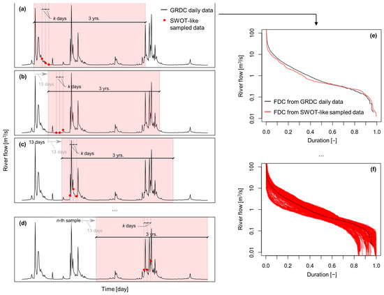
Figure 1.
Methodological scheme for the estimation of flow–duration curves (FDC) from SWOT-like river flow data. (a–d) SWOT-like river flow data sampled from observed GRDC time series every k days within a 3-year moving time frame (red areas). (e,f) Computation of FDCs, showing the comparison between the observed and SWOT-based FDCs within a single (e) or multiple time frames (f).
To account for possible satellite measurement errors, which may be due to, among others, atmospheric disturbance, actual river flow conditions spanning from low- to high-flow conditions, and random faultiness of the instrument, [25] suggests considering both biases and random errors, estimated around 30% and 20%, respectively. Given this, we assumed that SWOT-like river flows can be related to sampled GRDC data as follows:
where is the simulation of remotely sensed river flows from SWOT at the river gauge station j and time t, assuming a bias and a random error proportional to μ and σ, respectively, and a sampling recurrence equal to k days. More specifically, j amounts to 1200 river gauge stations in total and t ranges up to 3 years. is the GRDC river flow observation measured at the river gauge station j, at time t and sampled every k days. We assumed that the SWOT measurement errors followed a normal distribution with mean μ and standard deviation σ, where μ = 0, ±0.15, ±0.30 and σ = 0, ±0.20. Overall, we considered six possible perturbation scenarios, where river flows were either not perturbed or they were altered by minor or major biases triggering both over- and underestimations and by random errors in the detected magnitude (see Table 1 for a detailed list). For each perturbation scenario, we then defined four alternative sampling recurrences (i.e., k, ranging between 3, 5, 7, and 10 days). In total, 6 × 4 = 24 alternative SWOT-like river flow datasets were examined. We acknowledge that the simulation method may likely produce negative values in the simulated time series, but we assumed that these random occurrences might simulate missing values, which will be considered as NA (i.e., not available).

Table 1.
Description of SWOT-like river flow datasets, accounting for potential biases and random errors in estimating river flow values and considering alternative sampling recurrences.
2.3. Estimation of Flow–Duration Curves from SWOT-like River Flow Data
For a gauged site, the empirical FDC can be obtained from the daily river flow data by considering the entire record, pooled in one sample (i.e., period-of-record FDC), and by ranking in ascending order the river flow observations, which are associated with their corresponding duration (i.e., fractional or percentage). The duration di is equal to an estimate of the exceedance probability of the i-th observation in the sorted sample, 1-Fi. If Fi is estimated using a Weibull plotting position, the duration di is expressed as follows:
where i is the i-th position in the rearranged sample and N is the length of daily river flows observed in a gauged site.
Here, we computed FDCs using as input data SWOT-like river flows (Table 1, Figure 1), and we tested for their statistical representativeness with respect to FDCs from observed GRDC river flows. To this aim, the Nash–Sutcliffe efficiency index (NSE) and the mean relative error (MRE) were used.
Given a selected river gauge station j and a sampling recurrence k, for each 3-year-long SWOT time frame l, where the number of time frames Nl depends on the available GRDC observations, we computed NSE as follows:
where is the river flow quantile, as derived from the SWOT-based FDC, for the river gauge station j and duration di within a generic time frame l and sampled from GRDC data every k days; is the river flow quantile, as derived from the GRDC-based (i.e., observed daily river flows) FDC for the river gauge station j and duration di; is the mean of the GRDC-based river flow quantiles for the river gauge station j. For each river gauge station j (amounting to 1200), Nl values of NSE are computed, where the duration di ranges between 0 and 1 and is discretized in n = 366 points.
In order to assess the behavior across duration ranges, we estimated the mean relative errors (MREs) for three specific duration values, namely d = 0.027, d = 0.5, and d = 0.973, which are representative of high, median, and low flows, respectively. For a given river gauge station j and sampling recurrence k, the MRE values can be computed as follows:
where is the number of 3-year-long time frames for the river gauge station j, while other symbols are as above.
In order to interpret our results from a climatic perspective, and thus understand how and where SWOT-derived FDCs can better predict long-term flow–duration curves, we used the Köppen–Geiger climate classification [31]. This classification outlines five macro-climatic classes, then subdivides those into 30 sub-classes. For our analysis, we assumed that the first-order classification represented a satisfactory trade-off for the level of details we wanted to achieve. The macro-climatic regions here considered were tropical (A), arid (B), temperate (C), cold (D), and polar (E).
3. Results and Discussion
3.1. GRDC-Based FDCs Compliant with SWOT Mission Features
One initial accomplishment of this study was the creation and publication of a global dataset of period-of-record FDCs (referred to hereafter as FDCs for simplicity), constructed using freely accessible river flow records. From the combination of GDRC river flow data and the global river bankfull width database [29], we considered in total 1200 river gauge sections, which complied with our methodological requirements [30]. A bias toward a larger number of river gauge stations in North America and Europe was evident, mainly due to a lower availability of data from GRDC in the remaining continents. The considered river gauge stations showed a rather heterogeneous spatial distribution across different macro-climatic classes, as shown in Figure 2 and Table 2. More than 44% of stations were located in cold climates, followed by temperate (28%), tropical (18%), arid (9%), and polar (1%) zones. Despite the low representativeness of polar areas, we still considered river gauge stations located in this region in order to make the presented procedure as general and reproducible as possible. The temporal availability of observed river flow time series from GRDC presented some variability (Table 2), with the average series lengths ranging from approximately 36 years across tropical climates to 81 years in polar regions. Similarly, the magnitude of river flows was well-assorted (see average values of median and mean river flows for climate-grouped gauge stations in Table 2), thus allowing us to explore the potential performance of SWOT-like data in reproducing FDCs, spanning from lower to higher river flows.
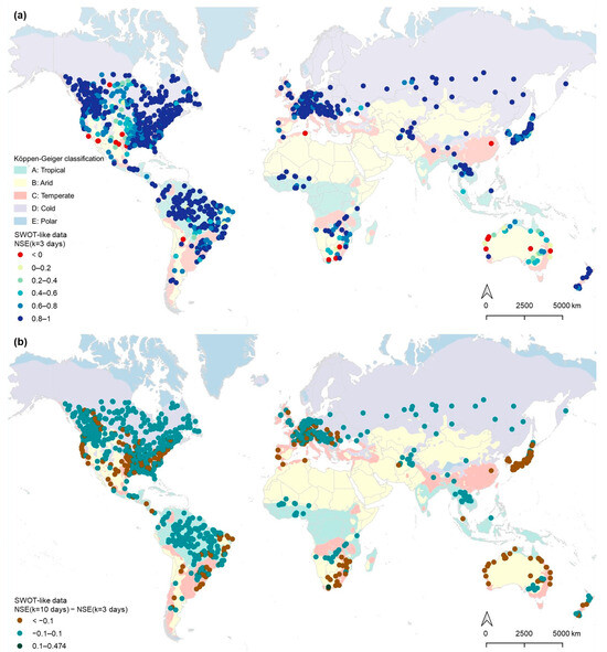
Figure 2.
Assessment of SWOT-like river flow data performance in reproducing long-term FDCs, expressed in terms of the Nash–Sutcliffe efficiency (NSE). The geographic location and the climatic characterization of the considered 1200 GRDC river gauge stations are also shown. (a) Values for the NSE computed from SWOT-like data derived from GRDC river flow observations without any bias or random error and sampled every 3 days (i.e., QSWOT,0,0,3). (b) Difference between NSE values computed from SWOT-like data derived from GRDC river flow observations without any bias or random error and sampled every 3 and 10 days (i.e., QSWOT,0,0,3 and QSWOT,0,0,10, respectively). Additional maps showing NSE values for the remaining SWOT-like river flow datasets are available in Appendix A.

Table 2.
Main characteristics of SWOT-like river flow series for different climatic macro-regions.
3.2. Creation of SWOT-like FDCs and Performance Analysis
As mentioned in the Methods, we defined 6 × 4 = 24 alternative SWOT-like river flow datasets, where 6 identifies the number of perturbation scenarios (i.e., whether river flows are not perturbed or if they are altered by minor or major biases triggering both over- and underestimations and random errors in the detected magnitude), and 4 represents the number of the considered sampling recurrences (i.e., k).
We evaluated the performance of SWOT-like data in reproducing FDCs compared to the observed daily river flows (Figure 2 and Figure A1, Figure A2, Figure A3, Figure A4, Figure A5 and Figure A6). As expected, our analysis revealed a marked heterogeneity of the performance of SWOT-based FDCs, which depends on the perturbation scenario, the satellite sampling recurrence, and the main climatic conditions.
In the case where we assumed that data from the ongoing SWOT mission were not affected by any bias or random perturbation and were sampled every 3 days (i.e., QSWOT,0,0,3, being the best-case scenario), the NSE values computed from the comparison against FDCs from the observed daily river flows presented some variability, with NSE > 0.8 for the majority of river gauge stations (Figure 2a). In the case the sampling recurrence was increased up to k = 10 days (i.e., QSWOT,0,0,10), a progressive decrease in NSE performances was found, as reported in Figure 2b, where we showed the difference in NSE values between k = 10 days and k = 3 days. Therein, 75% of river gauge stations presented ΔNSE values included in a ±0.1 range, with the majority of them (98%) showing underestimations. For the remaining 25% of stations, a larger NSE underestimation for QSWOT,0,0,10 was found compared to NSE values associated to QSWOT,0,0,3. It is evident that the NSE values dropped as the sampling recurrence k moved toward coarser sampling schemes, regardless of the macro-climatic conditions.
We grouped the NSE values according to the Köppen–Geiger macro-climates (Figure 3 and Table 3). Regardless of the sampling recurrence, the best reproduction (in terms of median values) of the observed FDCs as derived from the SWOT-like data without any perturbation (i.e., QSWOT,0,0,k) was observed in tropical climates, immediately followed by cold, polar, and temperate climates. As expected, arid climates showed significantly lower performances as they remarkably suffered from a reduction in the sampling recurrence, with median values of NSE lower than 0.75. Although river gauge locations belonging to the polar climate seemed to show rather high performances, the statistical significance of such a macro-climatic area could be misrepresented due to the low number of stations belonging to it. These stations are either mountainous catchments, likely located at high elevations, or at extreme latitudes. Nevertheless, our goal was to make the presented procedure as general and reproducible as possible, therefore we decided not to remove these sites from the analyses, which indeed would have introduced a further subjective rule.
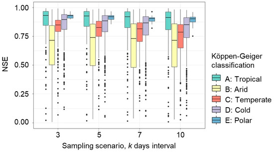
Figure 3.
Average site-specific NSE values, computed from SWOT-like data derived from GRDC river flow observations without any bias or random error (i.e., QSWOT,0,0,k) and grouped by macro-climate and sampling scenario. Additional boxplots showing NSE values for the remaining SWOT-like river flow datasets are available in Appendix A.

Table 3.
Median values of NSE, computed from SWOT-like data derived from GRDC river flow observations and grouped by macro-climate, perturbation, and sampling scenarios.
When looking at the variability of NSE values within each macro-climate, we found that tropical, temperate, and cold climates presented comparable interquartile ranges (IQR), significantly smaller than the IQR for arid climates. This once again suggests a possible poorer performance of SWOT data across arid regions. With increasing sampling time, we observed that temperate climates revealed a 63% increase in the IQR moving from k = 3 to k = 10 days sampling recurrence. Conversely, tropical and cold climates showed an overall lower variability, with little variations in the IQR (i.e., 41% and 47% IQR increase from k = 3 days to k = 10 days, respectively). Our results clearly highlight the large dependency of the performance of SWOT-based flow–duration curves on the particular climatic and regional area where river flow records are collected. For instance, in Japan, where two macro-climatic conditions exist within the same country (i.e., temperate in the south and cold in the north), we observed a rather amplified performance decline, mainly located in the southern part (Figure A1, Figure A2, Figure A3, Figure A4, Figure A5 and Figure A6). For river gauge stations located in mostly arid climates (e.g., in Australia, South Africa, or some limited parts of south-central United States), the variability in the SWOT-like data performance was higher than every other climatic condition, which may potentially suggest a lower reliability of SWOT-based FDCs across these regions.
In the case the SWOT data were characterized by random errors without any bias (i.e., QSWOT,0,20,k), and also in the case of negative biases (i.e., QSWOT,−15,20,k, QSWOT,−30,20,k), our analysis revealed that NSE performances (median values) tended to slightly worsen (Table 3 and Figure A7), showing lower median values, but comparable IQRs. Conversely, in the case positive biases were considered (i.e., QSWOT,15,20,k, QSWOT,30,20,k), the performance of SWOT-based FDCs decreased remarkably, with median NSE values ranging between 0.4 and 0.6 approximately. A detailed representation of NSE values for all the considered SWOT-like river flow datasets is reported in Figure A1, Figure A2, Figure A3, Figure A4, Figure A5, Figure A6 and Figure A7, where both the geographical and the climatic analyses are shown.
Despite NSE being a well-known metric that assesses the performance of modeled data compared to observations, it did not allow us to differentiate the performance analysis by distinguishing among different flow conditions (e.g., high and low flows). To this aim, we computed and analyzed the MRE values for relative durations equal to 0.027, 0.5, and 0.973 as representative of high, median, and low flow conditions, respectively.
We observed a general tendency of unperturbed SWOT-based FDCs (QSWOT,0,0,k) to satisfactorily mimic high and median flows, as shown by MRE values close to 0 and low IQRs (Figure 4a and Table 4). Indeed, in most rivers, lower baseflows tend to dominate the hydrograph (and thus the median) compared to flood flows because runoff peaks are fewer in number than baseflows between peaks. As a consequence, the average river flow would be biased low, while the median flow would be better represented. In particular, high flows revealed a slightly decreasing performance with increasing k values, characterized by higher MRE values and larger IQR with increasing k. This result was expected and highlights the importance of sampling river flows during floods with the highest sampling frequency as possible. Median flows looked less sensitive to varying sampling recurrences, as revealed by the overall uniform pattern across k values, and thus seem to be the most observable river flow regime for SWOT (Table 4). For median flows, the procedure delivered the narrowest IQRs in terms of MRE for all macro-climatic areas and sampling recurrence. When looking at low flows, SWOT-based FDCs tended to overestimate the observed FDCs, mainly due to less recurrent sampling. When comparing macro-climates, tropical areas revealed a better performance in terms of MRE, especially during low flows. As previously highlighted, arid climates presented the largest variability of median and low flows compared to all other climates.
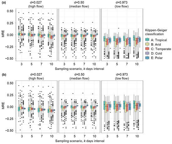
Figure 4.
Average site-specific mean relative error (MRE) values, computed from SWOT-like data derived from GRDC river flow observations (a) without any bias or random error (i.e., QSWOT,0,0,k), (b) assuming a random error only (i.e., QSWOT,0,20,k), and grouped by macro-climate and sampling scenario. Additional boxplots showing MRE values for the remaining SWOT-like river flow datasets are available in Appendix A.

Table 4.
Median values of MRE for median flows, computed from SWOT-like data derived from GRDC river flow observations and grouped by macro-climate, perturbation, and sampling scenarios.
In the case a random error characterized the SWOT-like data (i.e., QSWOT,0,20,k), our results showed a slight overestimation of high flows, with a pattern from k = 3 days to k = 10 days, similar to the one observed for unperturbed data (Figure 4b). Regarding low flows, a slight underestimation was detected, with larger IQRs, probably due to a smaller size of the river flow dataset (i.e., QSWOT < 0 is neglected). No remarkable changes were found for median flows.
Whether a negative (positive) bias will characterize the river flow estimates from SWOT, the MRE values tended to consistently increase (decrease), as shown in Table 4 and Figure A8. Despite this, our results proved that regardless of the potential bias of SWOT in estimating river flows, the distribution of MRE was not significantly affected. SWOT river flow estimations are expected to preserve the intrinsic variability of river flows even though a shift in the actual values may emerge, which needs to be properly assessed in order to provide reliable river flow estimates.
4. Conclusions
In anticipation of the upcoming release of SWOT products, this study investigated the mission potential to estimate flow–duration curves (FDCs) of remotely-sensed river flows. We examined the influence of sampling recurrences, biases, and random errors on river flow estimation, considering the most significant hydrological signatures of rivers (low, high, and median flows) and their climatic features.
In doing so, we also provide the first global collection of FDCs at traditionally monitored river sections (1200 gauging stations) using GRDC data with suitable consistency (i.e., length of records).
Our results show that the performance of SWOT-based FDCs heavily depends on the climatic and regional context of the rivers: the best median reproduction derived from unperturbed SWOT-like data occurred in tropical climates, closely followed by cold, polar, and temperate climates. Poor performance is expected in arid regions.
The sampling recurrence is also a significant factor, especially for high flows, where more frequent observations (i.e., k = 3) ensure a higher possibility to sample floods along the rivers. Among the considered flows, the median river flows result was less sensitive to varying sampling frequencies, as indicated by the overall uniform pattern across k values, making them the most reliably observable river flow regime for SWOT, regardless of the macro-climate conditions.
The presence of random errors or biases of SWOT data may significantly impact the errors on reproducing the river hydrological regime. Despite this, our results showed that the distribution of MRE remained largely unaffected by the presence of biases: SWOT is expected to maintain the intrinsic variability of river flows, although actual value shifts may occur. These results further highlight the relevance of the calibration/validation phase currently undertaken by the science mission teams, which should constrain the risk of random and unexpected biases.
This preliminary investigation paves the way for further studies. The promising performance of SWOT-based FDCs in depicting median flows offers potential for applications such as FDC regionalization (see, e.g., [9]), water management, habitat suitability, and other areas that rely on understanding river hydrological regimes and river flow variability.
Author Contributions
Conceptualization, A.D., S.C. and A.P.; Methodology, A.D., S.C. and A.P.; Software, S.C. and A.P.; Investigation, A.D., S.C. and A.P.; Data curation, A.P. and S.P.; Writing—original draft preparation, A.D., S.C., A.P. and S.P.; Writing—review and editing, A.D., S.C., A.P., S.P., I.P., A.C., A.M. and A.B.; Visualization, S.C. and A.P.; Supervision, A.D., A.C. and A.B. All authors have read and agreed to the published version of the manuscript.
Funding
This research received no external funding.
Data Availability Statement
Data supporting the reported results are available at https://doi.org/10.5281/zenodo.11257221, accessed on 24 May 2024.
Conflicts of Interest
The authors declare no conflicts of interest.
Appendix A
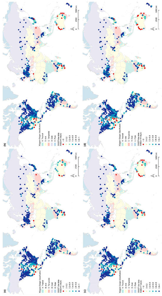
Figure A1.
Assessment of SWOT-like river flow data performance in reproducing long-term FDCs, expressed in terms of the Nash–Sutcliffe efficiency (NSE). The geographic location and the climatic characterization of the considered 1200 GRDC river gauge stations are also shown. Values for NSE computed from SWOT-like data derived from GRDC river flow observations without any bias or random error (i.e., Qswot,0,0,k) and sampled every (a) 3 days, (b) 5 days, (c) 7 days, and (d) 10 days.
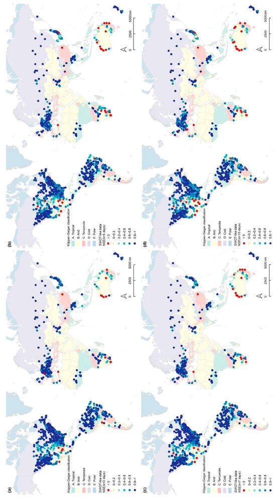
Figure A2.
Assessment of SWOT-like river flow data performance in reproducing long-term FDCs, expressed in terms of the Nash–Sutcliffe efficiency (NSE). The geographic location and the climatic characterization of the considered 1200 GRDC river gauge stations are also shown. Values for NSE computed from SWOT-like data derived from GRDC river flow observations considering a 20% random error (i.e., Qswot,0,20,k) and sampled every (a) 3 days, (b) 5 days, (c) 7 days, and (d) 10 days.
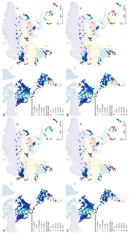
Figure A3.
Assessment of SWOT-like river flow data performance in reproducing long-term FDCs, expressed in terms of the Nash–Sutcliffe efficiency (NSE). The geographic location and the climatic characterization of the considered 1200 GRDC river gauge stations are also shown. Values for NSE computed from SWOT-like data derived from GRDC river flow observations considering a 15% negative bias and a 20% random error (i.e., Qswot,−15,20,k) and sampled every (a) 3 days, (b) 5 days, (c) 7 days, and (d) 10 days.
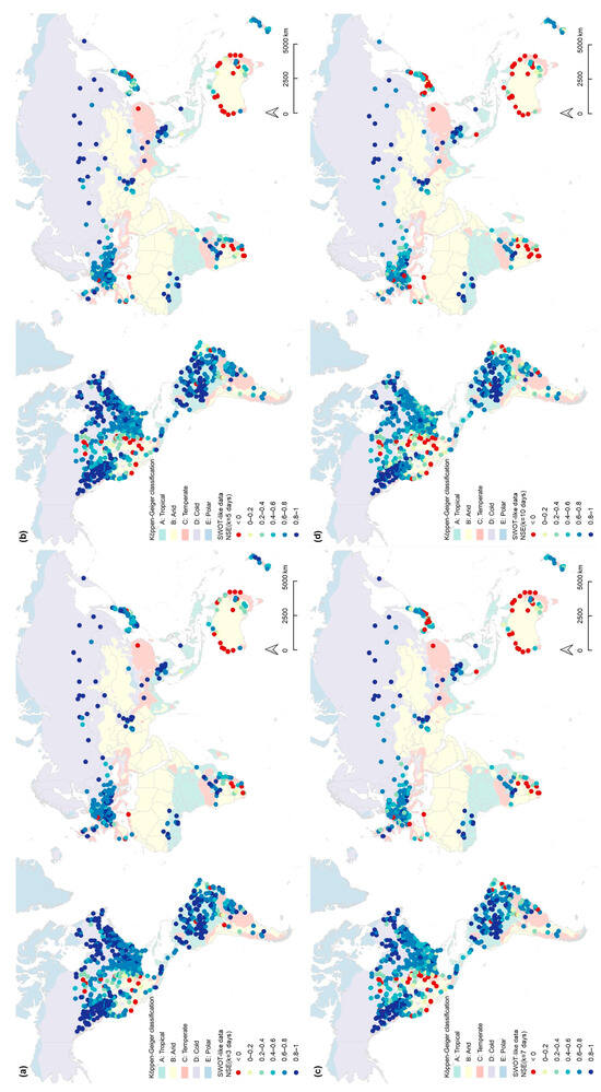
Figure A4.
Assessment of SWOT-like river flow data performance in reproducing long-term FDCs, expressed in terms of the Nash–Sutcliffe efficiency (NSE). The geographic location and the climatic characterization of the considered 1200 GRDC river gauge stations are also shown. Values for NSE computed from SWOT-like data derived from GRDC river flow observations considering a 15% positive bias and a 20% random error (i.e., Qswot,15,20,k) and sampled every (a) 3 days, (b) 5 days, (c) 7 days, and (d) 10 days.
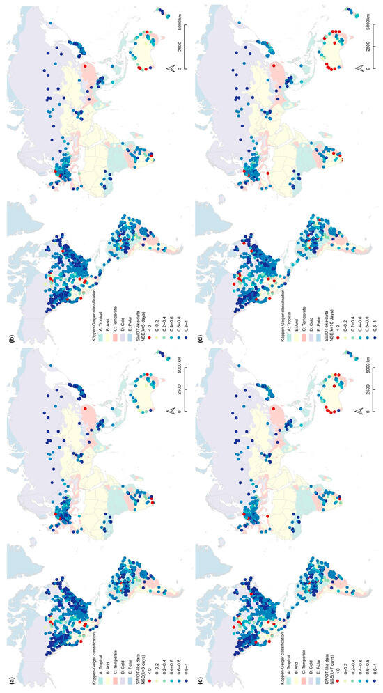
Figure A5.
Assessment of SWOT-like river flow data performance in reproducing long-term FDCs, expressed in terms of the Nash–Sutcliffe efficiency (NSE). The geographic location and the climatic characterization of the considered 1200 GRDC river gauge stations are also shown. Values for NSE computed from SWOT-like data derived from GRDC river flow observations considering a 30% negative bias and a 20% random error (i.e., Qswot,−30,20,k) and sampled every (a) 3 days, (b) 5 days, (c) 7 days, and (d) 10 days.
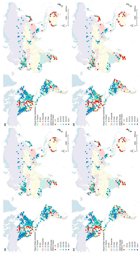
Figure A6.
Assessment of SWOT-like river flow data performance in reproducing long-term FDCs, expressed in terms of the Nash–Sutcliffe efficiency (NSE). The geographic location and the climatic characterization of the considered 1200 GRDC river gauge stations are also shown. Values for NSE computed from SWOT-like data derived from GRDC river flow observations considering a 30% positive bias and a 20% random error (i.e., Qswot,30,20,k) and sampled every (a) 3 days, (b) 5 days, (c) 7 days, and (d) 10 days.
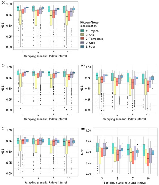
Figure A7.
Average site-specific NSE values, computed from SWOT-like data derived from GRDC river flow observations and grouped by macro-climate and sampling scenario for (a) 20% random error (Qswot,0,20,k), (b) 15% negative bias and 20% random error (Qswot,−15,20,k), (c) 15% positive bias and 20% random error (Qswot,15,20,k), (d) 30% negative bias and 20% random error (Qswot,−30,20,k), and (e) 30% positive bias and 20% random error (Qswot,30,20,k).
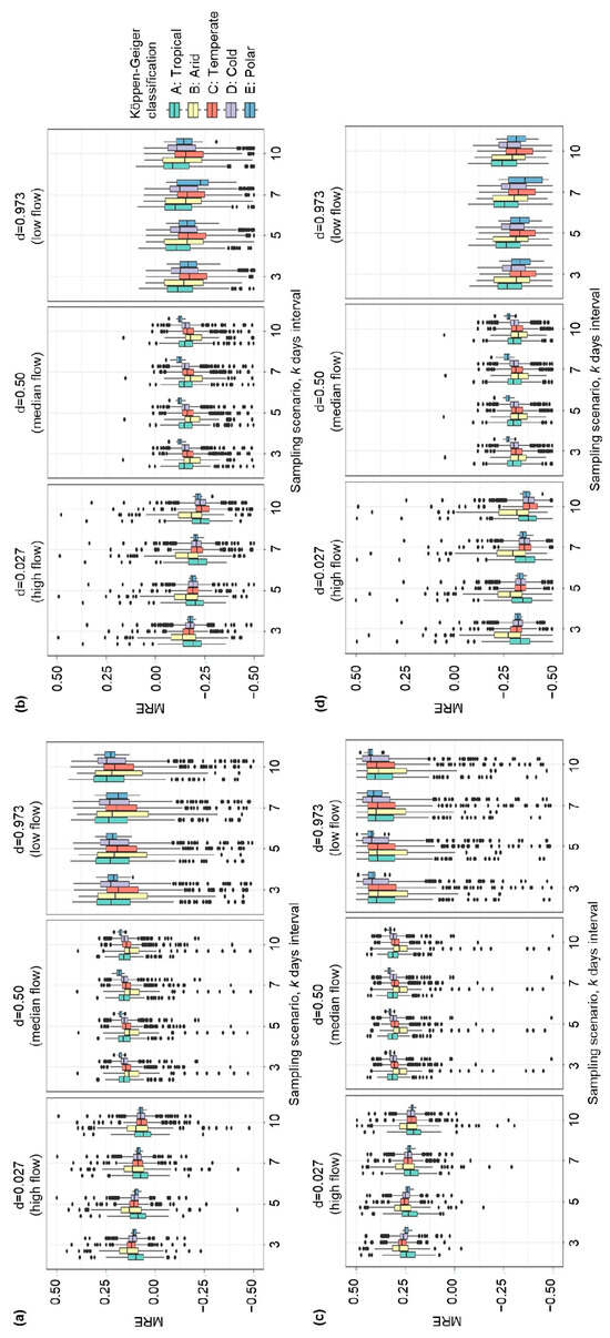
Figure A8.
Average site-specific mean relative error (MRE) values, computed from SWOT-like data derived from GRDC river flow observations and grouped by macro-climate and sampling scenario for (a) 15% negative bias and 20% random error (Qswot,−15,20,k), (b) 15% positive bias and 20% random error (Qswot,15,20,k), (c) 30% negative bias and 20% random error (Qswot,−30,20,k), and (d) 30% positive bias and 20% random error (Qswot,30,20,k).
References
- Krabbenhoft, C.A.; Allen, G.H.; Lin, P.; Godsey, S.E.; Allen, D.C.; Ryan, M.; Delvecchia, A.G.; Fritz, K.M.; Shanafield, M.; Burgin, A.J.; et al. Assessing Placement Bias of the Global River Gauge Network. Nat. Sustain. 2022, 5, 586–592. [Google Scholar] [CrossRef]
- Hall, J.; Arheimer, B.; Borga, M.; Brazdil, R.; Claps, P.; Kiss, A.; Kjeldsen, T.R.; Kriauciuniene, J.; Kundzewicz, Z.W.; Lang, M.; et al. Understanding Flood Regime Changes in Europe: A State-of-the-Art Assessment. Hydrol. Earth Syst. Sci. 2014, 18, 2735–2772. [Google Scholar] [CrossRef]
- Tourian, M.J.; Schwatke, C.; Sneeuw, N. River Discharge Estimation at Daily Resolution from Satellite Altimetry over an Entire River Basin. J. Hydrol. 2017, 546, 230–247. [Google Scholar] [CrossRef]
- Tourian, M.J.; Sneeuw, N.; Bárdossy, a. A Quantile Function Approach to Discharge Estimation from Satellite Altimetry (ENVISAT). Water Resour. Res. 2013, 49, 4174–4186. [Google Scholar] [CrossRef]
- Blöschl, G.; Bierkens, M.F.P.; Chambel, A.; Cudennec, C.; Destouni, G.; Fiori, A.; Kirchner, J.W.; Mcdonnell, J.J.; Savenije, H.G.; Sivapalan, M.; et al. Twenty-Three Unsolved Problems in Hydrology (UPH)—A Community Perspective. Hydrol. Sci. J. 2019, 64, 1141–1158. [Google Scholar] [CrossRef]
- Vogel, R.M.; Fennessey, N.M. Flow-Duration Curves. I: New Interpretation and Confidence Intervals. J. Water Resour. Plan. Manag. 1994, 120, 485–504. [Google Scholar] [CrossRef]
- Castellarin, A.; Galeati, G.; Brandimarte, L.; Montanari, A.; Brath, A. Regional Flow-Duration Curves: Reliability for Ungauged Basins. Adv. Water Resour. 2004, 27, 953–965. [Google Scholar] [CrossRef]
- Hughes, D.A.; Smakhtin, V. Daily Flow Time Series Patching or Extension: A Spatial Interpolation Approach Based on Flow Duration Curves. Hydrol. Sci. J. 1996, 41, 851–871. [Google Scholar] [CrossRef]
- Pugliese, A.; Persiano, S.; Bagli, S.; Mazzoli, P.; Parajka, J.; Arheimer, B.; Capell, R.; Montanari, A.; Blöschl, G.; Castellarin, A. A Geostatistical Data-Assimilation Technique for Enhancing Macro-Scale Rainfall—Runoff Simulations. Hydrol. Earth Syst. Sci. 2018, 22, 4633–4648. [Google Scholar] [CrossRef]
- Ceola, S.; Pugliese, A.; Ventura, M.; Galeati, G.; Montanari, A.; Castellarin, A. Hydro-Power Production and Fish Habitat Suitability: Assessing Impact and Effectiveness of Ecological Flows at Regional Scale. Adv. Water Resour. 2018, 116, 29–39. [Google Scholar] [CrossRef]
- Yaeger, M.; Coopersmith, E.; Ye, S.; Cheng, L.; Viglione, A.; Sivapalan, M. Exploring the Physical Controls of Regional Patterns of Flow Duration Curves—Part 4: A Synthesis of Empirical Analysis, Process Modeling and Catchment Classification. Hydrol. Earth Syst. Sci. 2012, 16, 4483–4498. [Google Scholar] [CrossRef]
- Kroll, C.N.; Croteau, K.E.; Vogel, R.M. Hypothesis Tests for Hydrologic Alteration. J. Hydrol. 2015, 530, 117–126. [Google Scholar] [CrossRef]
- Vogel, R.M.; Fennessey, N.M. Flow Duration Curves II: A Review of Applications in Water Resources Planning. JAWRA J. Am. Water Resour. Assoc. 1995, 31, 1029–1039. [Google Scholar] [CrossRef]
- Castellarin, A. Regional Prediction of Flow-Duration Curves Using a Three-Dimensional Kriging. J. Hydrol. 2014, 513, 179–191. [Google Scholar] [CrossRef]
- Persiano, S.; Pugliese, A.; Aloe, A.; Skøien, J.O.; Castellarin, A.; Pistocchi, A. Streamflow Data Availability in Europe: A Detailed Dataset of Interpolated Flow-Duration Curves. Earth Syst. Sci. Data 2022, 14, 4435–4443. [Google Scholar] [CrossRef]
- Castellarin, A.; Vogel, R.M.; Brath, A. A Stochastic Index Flow Model of Flow Duration Curves. Water Resour. Res. 2004, 40, 1–10. [Google Scholar] [CrossRef]
- Castellarin, A. Probabilistic Envelope Curves for Design Flood Estimation at Ungauged Sites. Water Resour. Res. 2007, 43, 1–12. [Google Scholar] [CrossRef]
- Ganora, D.; Claps, P.; Laio, F.; Viglione, A. An Approach to Estimate Nonparametric Flow Duration Curves in Ungauged Basins. Water Resour. Res. 2009, 45, 1–10. [Google Scholar] [CrossRef]
- Pugliese, a.; Castellarin, a.; Brath, a. Geostatistical Prediction of Flow–Duration Curves in an Index-Flow Framework. Hydrol. Earth Syst. Sci. 2014, 18, 3801–3816. [Google Scholar] [CrossRef]
- Gleason, C.J.; Durand, M.T. Remote Sensing of River Discharge: A Review and a Framing for the Discipline. Remote Sens. 2020, 12, 1107. [Google Scholar] [CrossRef]
- Rodriguez, E. Surface Water and Ocean Topography Mission (SWOT) Project Science Requirements Document; JPL D-61923; California Institute of Technology: Pasadena, CA, USA, 2015. [Google Scholar]
- Durand, M.; Gleason, C.J.; Pavelsky, T.M.; Prata, R.; Frasson, D.M.; Turmon, M.; David, C.H.; Altenau, E.H.; Tebaldi, N.; Larnier, K.; et al. A Framework for Estimating Global River Discharge From the Surface Water and Ocean Topography Satellite Mission Water Resources Research. Water Resour. Res. 2023, 59, e2021WR031614. [Google Scholar] [CrossRef]
- Fu, L.L.; Pavelsky, T.; Cretaux, J.F.; Morrow, R.; Farrar, J.T.; Vaze, P.; Sengenes, P.; Shiffer, N.V.; Baron, A.S.; Picot, N.; et al. Special Section: The Surface Water and Ocean Topography Mission: A Breakthrough in Radar Remote Sensing of the Ocean and Land Surface Water. Geophys. Res. Lett. 2024, 51, e2023GL107652. [Google Scholar] [CrossRef]
- Durand, M.; Gleason, C.J.; Garambois, P.A.; Bjerklie, D.; Smith, L.C.; Roux, H.; Rodriguez, E.; Bates, P.D.; Pavelsky, T.M.; Monnier, J.; et al. An Intercomparison of Remote Sensing River Discharge Estimation Algorithms From Measurements of River Height, Width, and Slope. Water Resour. Res. 2016, 52, 4527–4549. [Google Scholar] [CrossRef]
- Prata, R.; Frasson, D.M.; Durand, M.T.; Larnier, K. Exploring the Factors Controlling the Error Characteristics of the Surface Water and Ocean Topography Mission Discharge Estimates. Water Resour. Res. 2021, 57, e2020WR028519. [Google Scholar] [CrossRef]
- Frasson, R.P.D.M.; Turmon, M.J.; Durand, M.T.; Cédric, D.H. Estimating the Relative Impact of Measurement, Parameter, and Flow Law Errors on Discharge from the Surface Water and Ocean Topography Mission. J. Hydrometeorol. 2023, 24, 425–443. [Google Scholar] [CrossRef]
- Domeneghetti, A.; Tarpanelli, A.; Grimaldi, L.; Brath, A. Flow Duration Curve from Satellite: Potential of a Lifetime SWOT Mission. Remote Sens. 2018, 10, 1107. [Google Scholar] [CrossRef]
- Biancamaria, S.; Lettenmaier, D.P.; Pavelsky, T.M. The SWOT Mission and Its Capabilities for Land Hydrology. Surv. Geophys. 2016, 37, 307–337. [Google Scholar] [CrossRef]
- Andreadis, K.M.; Schumann, G.J.P.; Pavelsky, T. A Simple Global River Bankfull Width and Depth Database. Water Resour. Res. 2013, 49, 7164–7168. [Google Scholar] [CrossRef]
- Leopold, L.B. A View of the River; Harvard University Press, Ed.; Harvard University Press: Cambridge, MA, USA, 1994. [Google Scholar]
- Beck, H.E.; Zimmermann, N.E.; Mcvicar, T.R.; Vergopolan, N.; Berg, A.; Wood, E.F. Present and Future Köppen-Geiger Climate Classification Maps at 1 -Km Resolution. Sci. Data 2018, 5, 180214. [Google Scholar] [CrossRef]
Disclaimer/Publisher’s Note: The statements, opinions and data contained in all publications are solely those of the individual author(s) and contributor(s) and not of MDPI and/or the editor(s). MDPI and/or the editor(s) disclaim responsibility for any injury to people or property resulting from any ideas, methods, instructions or products referred to in the content. |
© 2024 by the authors. Licensee MDPI, Basel, Switzerland. This article is an open access article distributed under the terms and conditions of the Creative Commons Attribution (CC BY) license (https://creativecommons.org/licenses/by/4.0/).