1. Introduction
In recent years, the domain of simultaneous localization and mapping (SLAM) [
1] has been an integral part of autonomous navigation, especially in environments where the reception of global navigation satellite system (GNSS) signals is unreliable or absent and where dynamic environmental conditions are the norm. SLAM aims to determine a robot’s pose while simultaneously generating a map of its environment using onboard sensors. This process occurs in environments that may be unknown or partially known. The diversity of applicable sensors in use has naturally led to the bifurcation of SLAM into two primary SLAM categories: LiDAR-based SLAM and visual SLAM. Visual SLAM encompasses various subtypes, including monocular, stereo, and RGB-D [
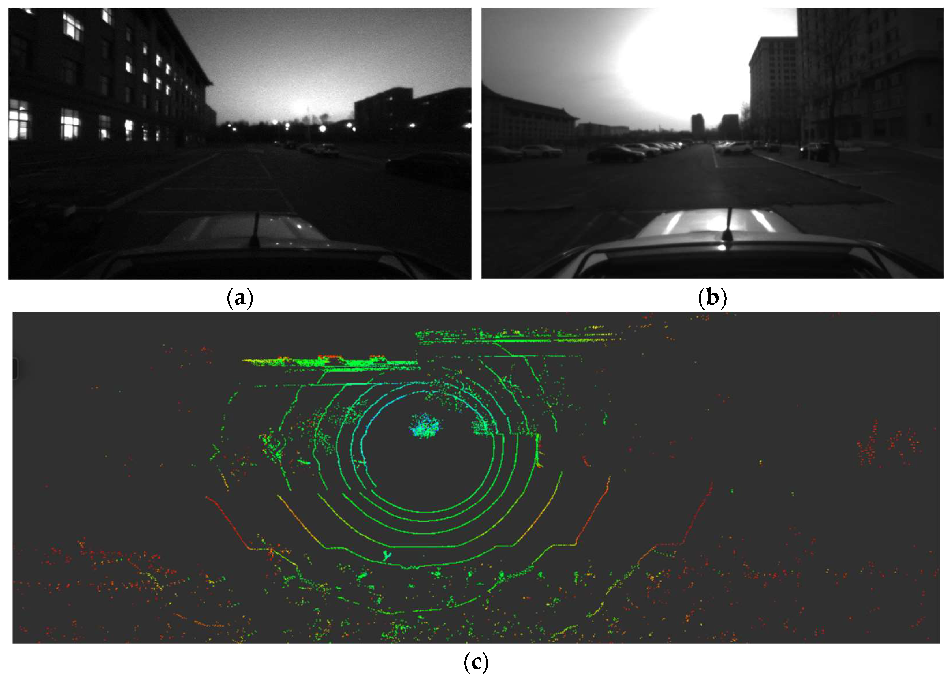
2]. LiDAR-based approaches demonstrate superior accuracy in pose estimation and maintain robust performance across varying environmental conditions, such as time of day and weather. In contrast, visual SLAM, as illustrated in
Figure 1, is highly susceptible to factors like lighting and the availability of distinctive features, thus potentially limiting its effectiveness in certain settings [
3]. Therefore, this paper concentrates on navigation systems leveraging LiDAR technology.
The last two decades have witnessed significant strides in LiDAR-based SLAM methodologies, fueled by advancements in computer processing power and optimization algorithms. While machine learning-based LiDAR SLAM methods are constrained by the scope and quality of training data, two primary categories dominate the current landscape: normal distributions transform (NDT) [
4] and iterative closest point (ICP) [
5] algorithm. The NDT approach, which has seen extensive application in 2D LiDAR SLAM scenarios, entails the discretization of the point cloud data into a grid-like structure, the computation of Gaussian distributions for each cell, and subsequent alignment-based matching and fitting procedures [
4]. However, the transition from 2D to 3D applications has exponentially increased computational demands, posing a significant challenge in meeting the stringent requirements for real-time processing [
6]. To put it simply, when classified solely based on the quantity of point clouds and meshes, the computational data of the most basic 3D LiDAR are at least 16 times that of a 2D LiDAR, as they have at least 16 scanning projection planes. Although efforts to mitigate this issue have been made through algorithms such as SEO-NDT [
7] and KD2D-NDT [
8], they have occasionally resulted in trade-offs concerning accuracy and processing time in certain scenarios. ICP-based methods face similar challenges. However, the advent of LiDAR odometry and mapping (LOAM) [
9] has marked a pivotal shift in focus; LOAM focuses the iteration process towards feature-rich points rather than the entire point cloud. This paradigm shift has propelled the widespread implementation of LOAM-inspired ICP techniques in addressing LiDAR SLAM challenges over the past decades.
LOAM distinguishes itself from conventional ICP techniques by classifying points in the point cloud based on their smoothness. This involves identifying and extracting “edge points”, which are characterized by coarse texture, and “planar points”, which exhibit fine texture. Subsequently, the derived feature points are systematically selected through a sector-based averaging technique. The system leverages these refined point clouds; the system performs odometry calculations at a frequency of 10 Hz using LiDAR data. Following the odometry computation, the aggregated point clouds are then employed for mapping at a reduced frequency of 1 Hz, thereby achieving a more accurate and efficient representation of the environment. To address LOAM’s limitations in computational demands and loop closure, Shan and Englot proposed LeGO-LOAM [
10]. This method, which stands for lightweight and ground-optimized LiDAR odometry and mapping, is specifically tailored for real-time six-degrees-of-freedom pose estimation with ground vehicles. However, further experiments have shown that the strategy of entirely segregating ground points from the surrounding point cloud environment for separate matching can result in a notable vertical drift. Furthermore, the methodologies for loop closure still face certain challenges.
Li He and colleagues investigated the application of Multiview 2D projection (M2DP) [
11] to describe 3D points to achieve loop closure, but their findings showed limited scope and efficacy. Scan Context [
12] and its advanced iteration, Scan Context++ [
13], were introduced by Giseop Kim in 2018 and 2021, respectively. These innovative approaches have rapidly gained recognition as leading solutions for loop closure in 3D LiDAR-based SLAM. This is a non-histogram-based global descriptor that directly captures egocentric structural information from the sensor’s field of view without relying on prior training. However, the aforementioned methods and their derivatives, such as F-LOAM [
14], do not utilize strapdown inertial navigation systems (SINSs) or only use them for the rectification of LiDAR point clouds.
Compared to the mature field of vision-aided SINS, the integration of SINS and LiDAR within LiDAR-based SLAM algorithms remains largely unexplored. A study [
15] employed a loosely coupled extended Kalman filter (EKF) to fuse IMU and LiDAR data within a two-dimensional framework. However, this approach lacked the robustness to handle the complexities of three-dimensional or multifaceted environments. Furthermore, a scholarly review published in 2022 [
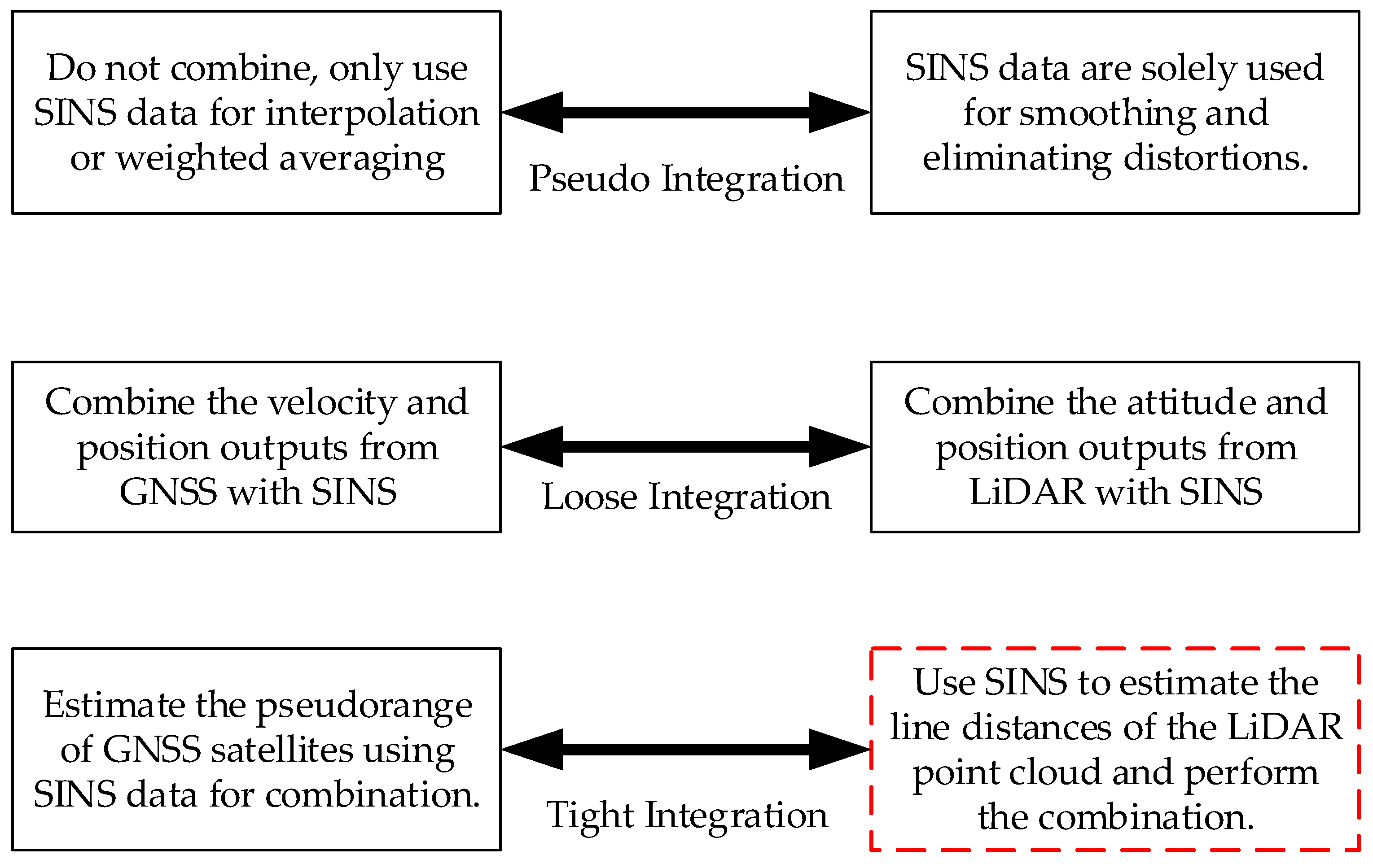
16] emphasized that within the majority of current systems employing the SINS/LiDAR integration systems, the SINS primarily functions to smooth trajectories and mitigate distortions. IMU data are often optionally integrated to predict platform motion and enhance registration accuracy during abrupt maneuvers. However, only gyroscopic measurements between consecutive LiDAR scans are utilized. Although these studies and related works often self-identify as “loose integration” based on the data fusion strategies outlined in this article, a more accurate designation would be “pseudo integration”.
As illustrated in
Figure 2, the concept of loose integration in LiDAR/SINS systems can be redefined from the GNSS/SINS loose integration navigation system. This approach involves combining position and other navigation data obtained from different sensors. In this process, none of the sensors involved in the integration have undergone in-depth data integration, but only a simple integration of the navigation results. By applying this redefined concept of loose integration, it becomes evident that studies such as [
17,
18], while claiming to employ tight integration, actually align more closely with the characteristics of loose integration. Specifically, these studies treat the individual systems as black boxes, focusing solely on integrating their outputs to generate the final navigation solution rather than performing in-depth data extraction and analysis.
To achieve a deeper level of sensor fusion than loose integration, the integration process should occur before the generation of individual navigation solutions. For instance, in a GNSS/SINS system, this translates to integrating data during the pseudorange measurement stage, prior to GNSS position determination. A key advantage of tightly coupled GNSS/SINS integration [
19] over the loosely coupled approach is its reduced reliance on a high number of visible satellites. This integration scheme can function even with a single observable satellite, unlike loose integration, which typically requires at least four. Investigating tight integration within SLAM systems necessitates understanding the nature of the data employed for navigation. In LiDAR-based systems, these data comprise point clouds, while vision-based systems utilize feature point information. Some studies [
20,
21] have demonstrated that within the SLAM framework, the concept of lines exhibits greater stability than points, particularly during data transformations (rotation and translation) across multiple frames. Similarly, research on multi-frame feature tracking within multi-state constrained Kalman filters for vision-aided inertial navigation [
22] has validated the enhanced accuracy and robustness of this approach compared to traditional methods. This has led to the development of a prototype tightly integrated LiDAR/SINS navigation system that utilizes line features extracted from the LiDAR point cloud as observations. The system employs continuous, multi-frame tracking of these line features to refine the SINS data. However, due to the sparse nature of the LiDAR point cloud, it is difficult to accurately track the same line. Consequently, revisiting the concept of distance as a measurement, akin to its application in GNSS/SINS systems, becomes crucial. Notably, distance, being a scalar quantity, offers a significant advantage—rotational invariance. This property can substantially reduce the computational burden of the integration process. The algorithm’s core principle centers on leveraging shared features, specifically line distances, across multiple frames to enhance Kalman filter accuracy. In summary, this paper presents the following contributions:
This paper refines the edge point extraction process of the LOAM algorithm by implementing a more granular clustering approach. By classifying clustered edge points as either convex or concave, the mapping precision is enhanced. Leveraging the rotational invariance of line distances, a Kalman filter is developed that employs line distance error as its primary observation metric. This approach improves the system’s robustness and accuracy.
This paper presents structural modifications to the LOAM algorithm that are predicated on the Scan Context framework to optimize its performance and ensure the data processing occurs more efficiently. The experiments have proven that the situation of incorrect loop closures in LiDAR SLAM has been mitigated effectively.
Extensive experiments conducted in various on-campus and off-campus environments validate the proposed algorithm and offer comparisons with traditional methods. These experiments highlight the superior performance of the proposed algorithm.
2. Method
This section outlines the workflow of our algorithm. This includes an insightful overview of the foundational principles that govern the pertinent hardware components, coupled with a thorough elucidation of the methodologies employed for the preprocessing of data.
Section 3 will then delve into the system error model and measurement model, providing a comprehensive analysis of these crucial framework elements. Additionally, to elucidate the algorithmic details, the subsequent sections of this paper will operate under the assumption that the LiDAR point cloud was sourced from a 16-line LiDAR system by default. This is representative of commonly used systems such as Velodyne’s VLP-16 (Velodyne Acoustics GmbH, Hamburg, Germany) and the LeiShen MS-C16 [
23] (Leishen Intelligent System Co., Ltd., located in Shenzhen, China) employed in the experiments of this paper. These systems, with a horizontal angular resolution of 0.2° and a vertical resolution of 2°, generate a range image of 1800 by 16 pixels [
23]. This translates to a point cloud with 16 projection planes, each containing 1800 points.
2.1. Algorithm Overview
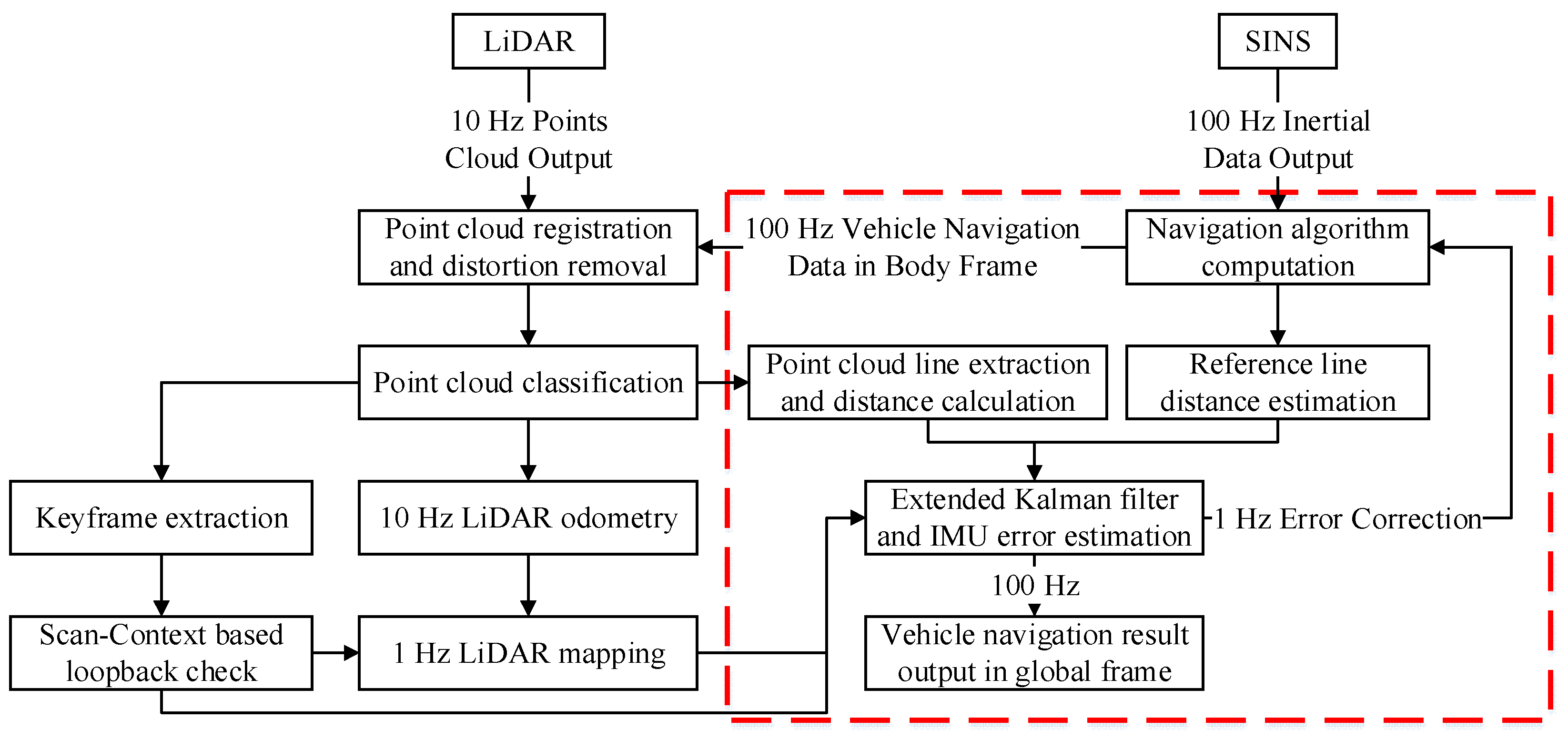
Figure 3 provides the overview of a tightly integrated LiDAR/SINS SLAM algorithm. Let
be the original points received in a laser scan. However, because scanning occurs over a timeframe t (typically exceeding 0.1 s), the resulting point cloud represents the environment over this duration rather than instantaneously. Consequently, in dynamic environments, the recorded point cloud may exhibit distortions caused by movements, particularly pronounced during significant angular variations. To mitigate this, it is essential to utilize the high-frequency motion data provided by the SINS to project all points onto the reference timestamps, either the beginning of the period
or the end
.
After processing, the point cloud is denoted as and proceeds to the next stage. Here, each point undergoes a meticulous classification into four categories based on its properties: (a) ground points, representing the surface on which the vehicle travels; (b) planar points, indicative of flat surfaces except the ground; (c) edge points, which demarcate boundaries or the perimeter of objects; and (d) the others, encompassing all points that do not fit into the previous categories. The subsequent section will elaborate on the point cloud classification technique, ensuring a thorough understanding. All points outside the ground in a key frame are compressed into scan context descriptors, and the key frames are set based on distance and the structure of the point clouds. Concurrently, after the clustering process, edge points are re-extracted to form edge lines. These edge lines will then serve as a basis for further computation of the reference line distances and facilitate tightly coupled filtering.
The LiDAR/SINS odometry primarily relies on the SINS navigation results, and the outputs further processed by LiDAR mapping, which matches and registers the undistorted point cloud onto a map at a frequency of 1 Hz. The Scan Context system performs loop closure detection based on both time and the distance traveled. When the similarity measure in the loop closure detection reaches a certain threshold, it is considered that the vehicle has returned to a previously visited location. Subsequently, the system optimizes the overall trajectory using this information. Successful loop closure detections will also contribute to the refinement of the SINS navigation and Kalman filtering processes.
2.2. Point Cloud Classification and Point Cloud Lines Extraction
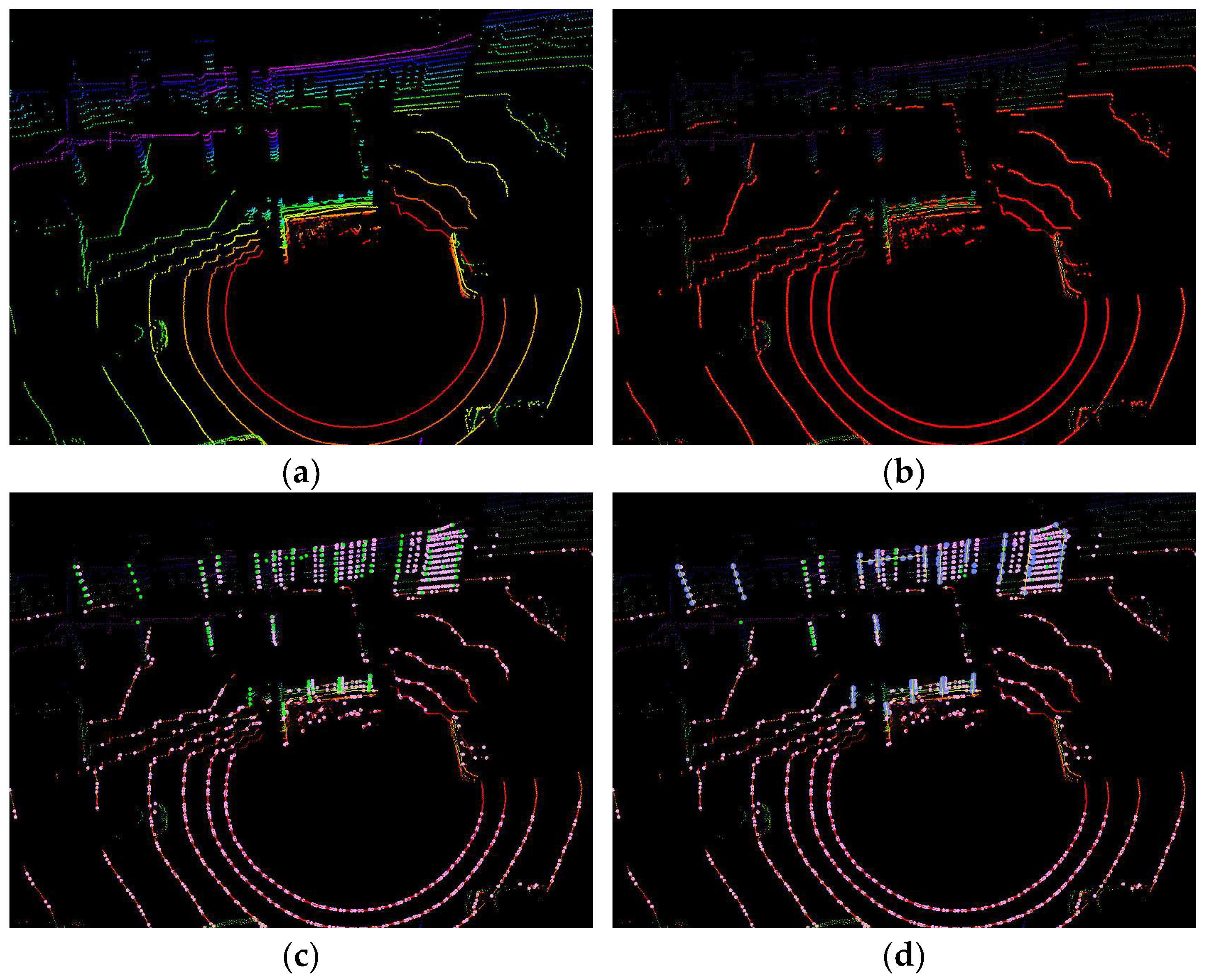
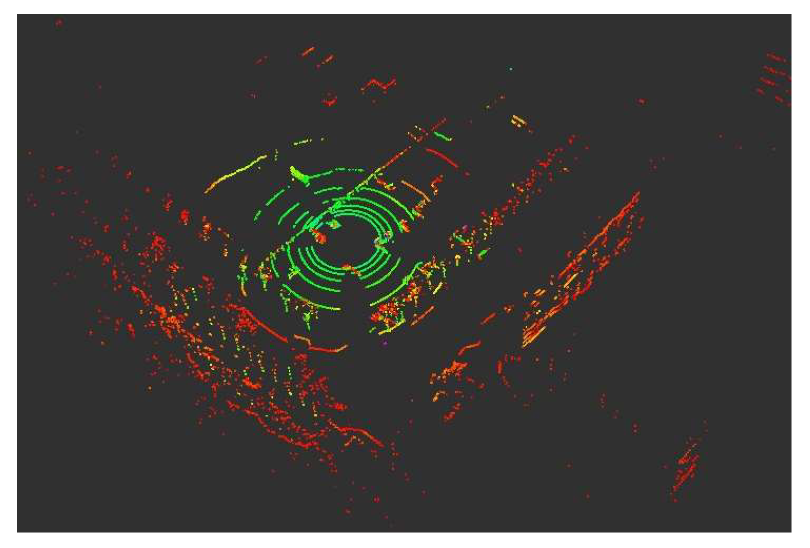
Figure 4 shows the undistorted raw point cloud, ground points, edge points, and planar points, as well as edge line points, respectively. The following will detail the extraction methods for each point type.
2.2.1. Ground Points
LeGO-LOAM employs a straightforward and efficient ground point extraction method, which involves specifically examining the 8 lines out of the total 16 that are positioned below 0° for detection [
23].
In point cloud
, point clouds are labeled with rings and scan sequence; let
,
As shown in
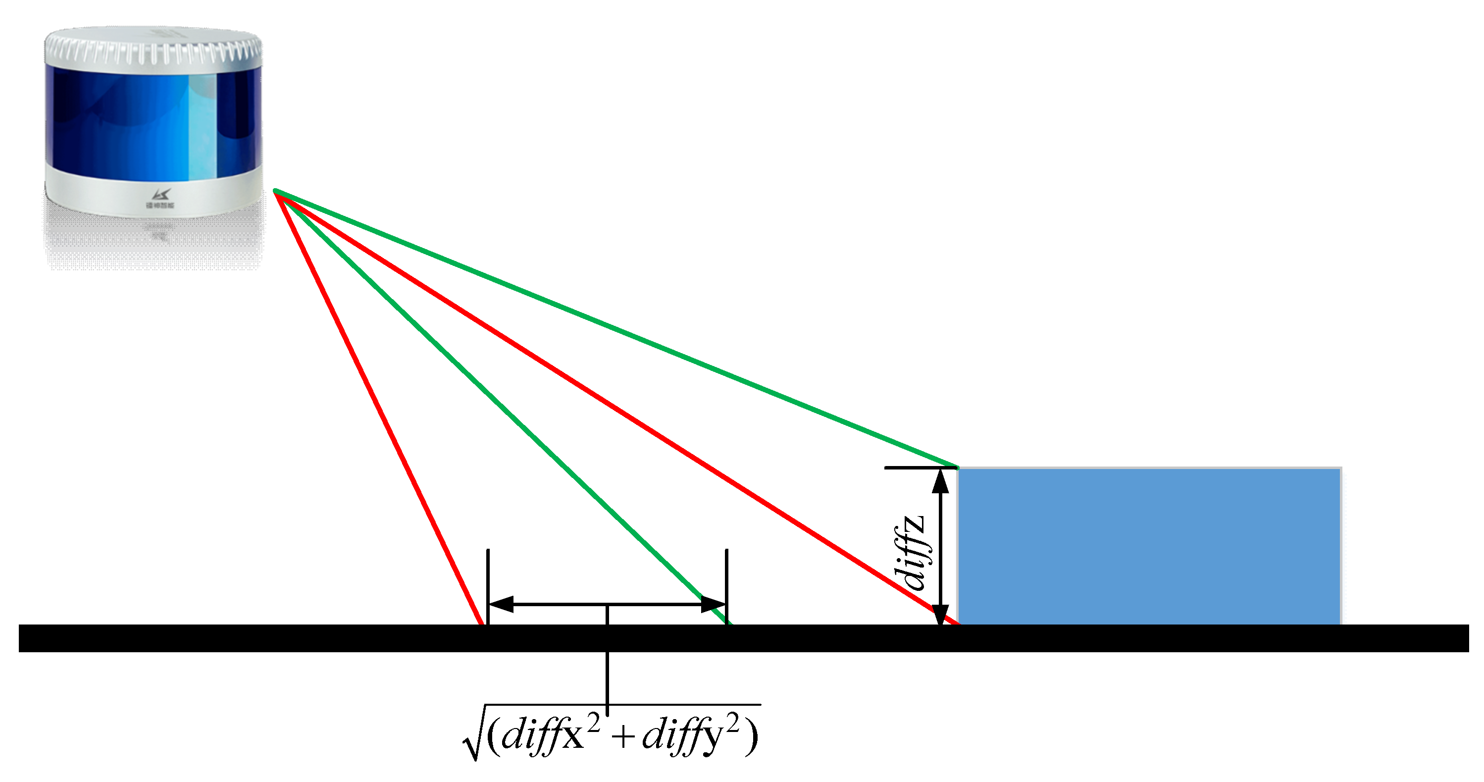
Figure 5, to calculate the angle between adjacent points
and
, this paper assumes their coordinate differences are denoted as
and
. The angle
could be set as:
Once
, points are marked as candidate ground points. Furthermore, an advanced point cloud sieving process [
24] will utilize the RANSAC (random sample consensus) [
25] technique to confirm the identification of ground points. This step is critical to avoid the misclassification of non-ground points as ground points, thereby ensuring the accuracy and reliability of the ground detection process. The fitted ground equation is as follows:
Then, an image-based segmentation method [
26] is applied to the range image to group points into many clusters. Points from the same cluster are assigned a unique label.
2.2.2. Edge and Planar Points
The feature extraction process is similar to the method used in [
9]; but, instead of extracting from the raw point cloud
, we exclusively utilize the portion of the point cloud that remains unmarked as ground points. Let
be the set of points of
from the same ring of the point clouds. Half of the points are on either side of
. The set for this paper is presented in
Table A1. Using the range values computed during segmentation, we can evaluate the roughness of point
in
,
where
means the range from
to the center of LiDAR.
Similar to LOAM, we use a threshold to distinguish different types of features. We call the points with larger than edge points, and the points with smaller than planar points. Then, we sort the edge and planar points from minimum to maximum. The point cloud is segmented into several distinct parts, and a specific number of feature points are extracted from within each segment.
Following the extraction of feature points, another attribute will be computed, specifically, the concavity or convexity of the edge points.
Figure 6 shows the difference between the concave points and convex points. Compare the distances between a specific point
and the remaining points within set
. If the majority of these points have distances greater than that of
, then
is considered a convex point. Otherwise, it is a concave point.
2.2.3. Edge Lines
After classifying edge points as concave or convex, this paper employs K-means clustering [
27] to group them into lines. Similarly, these lines will inherit concavity or convexity from the points that constitute them. This choice of using edge lines instead of individual edge points for subsequent computations stems from the inherent sparsity of LiDAR point clouds. Ensuring the capture of the exact same point across consecutive scans is a challenging proposition. In contrast, lines, when considered as collective entities, offer a higher degree of continuity and are much more amenable to persistent tracking. This approach enhances the reliability and robustness of the subsequent processing steps.
Section 3 will elaborate on the method for calculating point-to-line distances and the line selection criteria.
2.3. Scan Context
Scan Context was inspired by Shape Context [
28], proposed by Belongie et al.; it is an algorithm for place recognition using 3D LiDAR scans. It works by:
Partitioning the point cloud into bins based on azimuthal and radial directions.
Encoding the point cloud into a matrix where each bin’s value is the maximum height of points within it.
Calculating similarity between scan contexts using a column-wise distance measure.
Employing a two-phase search for loop detection that is invariant to viewpoint changes.
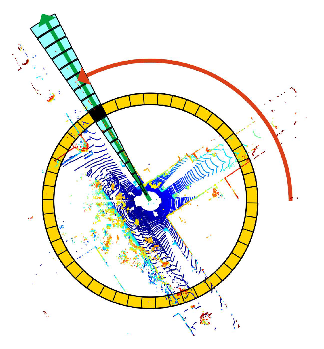
Figure 7 shows the bin division along azimuthal and radial directions. Using the top view of a point cloud from a 3D scan, the paper [
10] partitioned ground areas into bins, which were split according to both azimuthal (from 0 to 2π within a LiDAR frame) and radial (from center to maximum sensing range) directions. They referred to the yellow area as a ring, the cyan area as a sector, and the black-filled area as a bin.
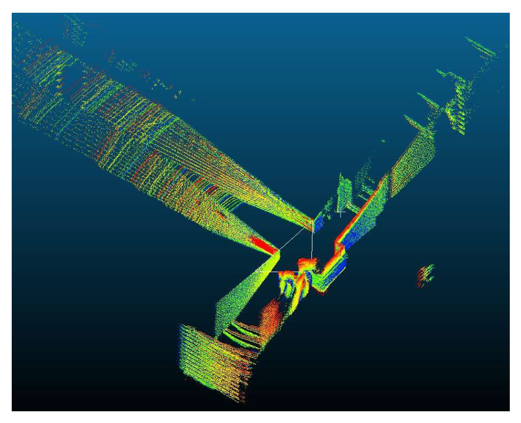
However, assigning the maximum height of points within a bin a value in the scan context can be problematic in certain situations. As depicted in
Figure 8, due to the formation principle of LiDAR point clouds, the point cloud does not fully unfold at close ranges, which may result in the highest point not accurately representing the actual environmental point cloud.
A straightforward and effective solution is to perform a ring-based search for the highest point. If the highest point lies within the outermost ring of the 3D LiDAR and is lower than the adjacent bins, an additional annotation is made to record that the highest point has not been detected. The marked bin can then serve as a ring-key in scan context for the initial match.
Simultaneously, because the point cloud distribution is dense near and sparse far, for each point cloud P selected as a key frame, we can first calculate its centroid:
where
is the total number of the point cloud and
is the point cloud
transformed back to the center of the original point cloud.
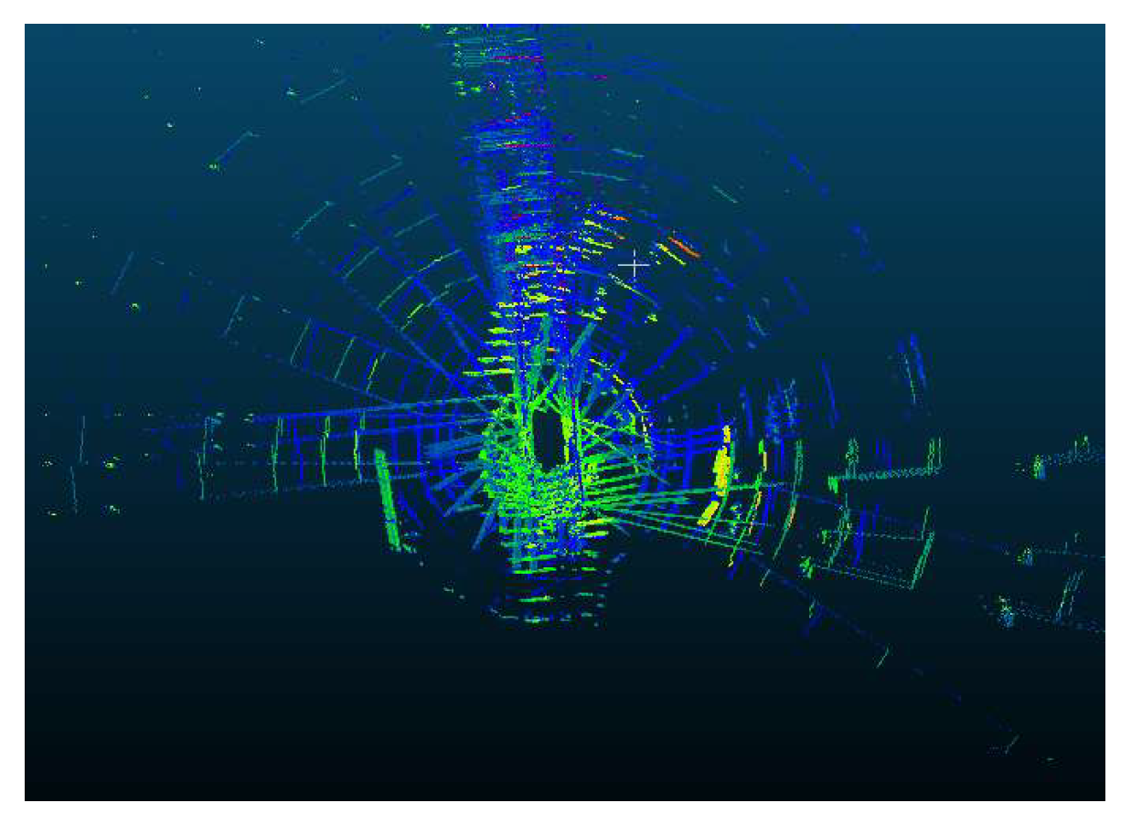
As is shown in
Figure 9, the transformed point cloud will have a common center, which will save a significant amount of time in subsequent scan context description and matching processes.
3. LiDAR/SINS System Model
3.1. System Error Model
The SINS integrated navigation system error model was designed following the list in [
29]:
The specific parameters in Equation (6) can be referred to in Equation (A1). And and are local latitude and longitude. and are meridian radius and normal radius. The is the geodetic height. is the transformation matrix from body frame to navigation frame.
For system state variables, , denotes the positional errors in longitude, latitude, and height. presents the velocity errors related to the three directions above. is the error attitude. and are the sensor noise errors of the gyroscopes and accelerometers, respectively.
The
is system noise, and the corresponding system noise matrix is given by:
where
,
and
denote reciprocals of the correlation times of the autocorrelation sequence of
while
,
and
are related to
. The
,
,
,
,
and
are variance associated with gyroscope and accelerometer errors.
3.2. The Observation Model
Traditionally, LiDAR-IMU integration has followed a loosely coupled approach. The observation variables of the model defined as the estimated position errors are:
However, this integration approach merely treats LiDAR and SINS as two black boxes, simply combining their output results without any deeper level of mutual correction. This paper draws on the concept of tight integration between GNSS and SINS, selecting the error of the reference line distance as the observation variable for filtering.
The selection of the error of as the observation variable is based on the following considerations:
Frame invariance: In navigation systems, the relative orientation between the body frame and the navigation frame continuously changes. Distance, however, remains consistent across different frames.
Robustness to data loss: Compared to vision data, LiDAR point clouds are inherently sparse. Using feature points and their associated information directly as observation variables increases the susceptibility to data loss.
In three-dimensional space, the distance from a point
to a straight line that was built by points
and
can be calculated as follow:
Imagine the points
L1 and
L2 with coordinates
and
, respectively, and the origin of the vehicle or robot in time
could be estimated as
while the ground truth is
; the relationship between them is:
where
and
are the position errors in the ENU directions and
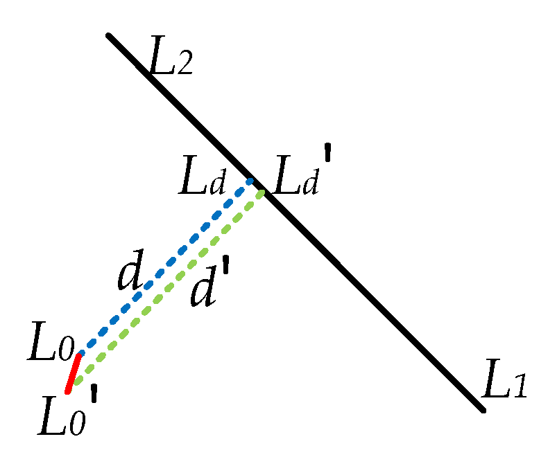
. The figure above represents the relationship between the vehicle and the reference line in three-dimensional space, where
denotes the actual position of the vehicle and
signifies the vehicle’s estimated position.
The measurement parameter in the EKF system is:
As is shown in
Figure 10,
is much smaller than
or
; it can be approximately considered that the normal vector to the line
connecting
and
is consistent. Then, the relationship between
and
could be set as follows:
is the normalized vector from
. Meanwhile, the corresponding system design matrix
is:
is the number of reference lines selected in the integrated system. It will always be changed with the changing of point clouds.
For the LiDAR/IMU EKF system, the formulation linking the system observation variables and state variables is:
,
, and
were defined previously and
represents the observation noise. As mentioned above, the LiDAR point cloud is the covariance value of
. LiDAR point clouds exhibit sparsity, and the uncertainty of a single point affects its entire surrounding space. The surrounding space is a truncated segment of a torus. For ease of calculation, this paper assumes it to be a rectangular prism, and its volume represents the covariance value of the measurement noise
.
For example, imagine a special distance of the reference line . The covariance value of the noise of is and is the horizontal separation angle of the LiDAR device while is the vertical separation angle.
As mentioned above, refers to the number of reference lines; in this stated equation, this paper proposes that the following principles should be adhered to in controlling the reference lines involved in the filtering process.
Region division: The point cloud is segmented into multiple regions based on the scanning direction. Each region is characterized by the edge lines exhibiting distinct convexity/concavity properties.
Reference line tracking: The position of each reference line is tracked across multiple frames using SINS transformations. This ensures the consistent matching of the same reference line over an extended period.
Dynamic reference line management: Due to the inherent sparsity of point clouds, reference lines exceeding a predefined distance threshold are discarded. New reference lines are introduced to maintain robust matching.
3.3. Tracking of Reference Lines
The selection rules of the reference lines are mentioned in
Section 3.2. Here, the tracking of these lines will be revealed with details.
As mentioned in
Section 2.3, scan context built a series of point bins to extract the point cloud information. Imagine the attitude transformation matrix during the tracking period is
while the
represents the displacement provided by SINS. The projections
,
of points
and
in the new point cloud could be calculated in Equation (12):
Connect
and
to obtain the scan context bins they pass through. By statistically analyzing these bins with their adjacent bins, select the edge line
that is also located in the same bin area. To further determine whether it is derived from a change in the original edge line, in addition to judging its concavity and convexity as well as the concavity and convexity and distance of the closest edge line, a further similarity analysis can be conducted on the line vectors.
The smaller the value of
, the higher the similarity between the two lines is. Based on the above conditions, it can be determined whether the new edge line is the target that needs to be tracked. The final threshold selection for this paper can be referred to in the data presented in
Table 1.
5. Discussion
5.1. Results’ Interpretation and Contribution
It redefines the fundamental computational unit in LiDAR SLAM by shifting the focus from LiDAR regression to an INS, rather than treating it as merely an accessory to LiDAR. The high-frequency output from the SINS navigation significantly reduced the computational load on the odometry component of LiDAR SLAM, thereby enhancing the accuracy of its positioning results.
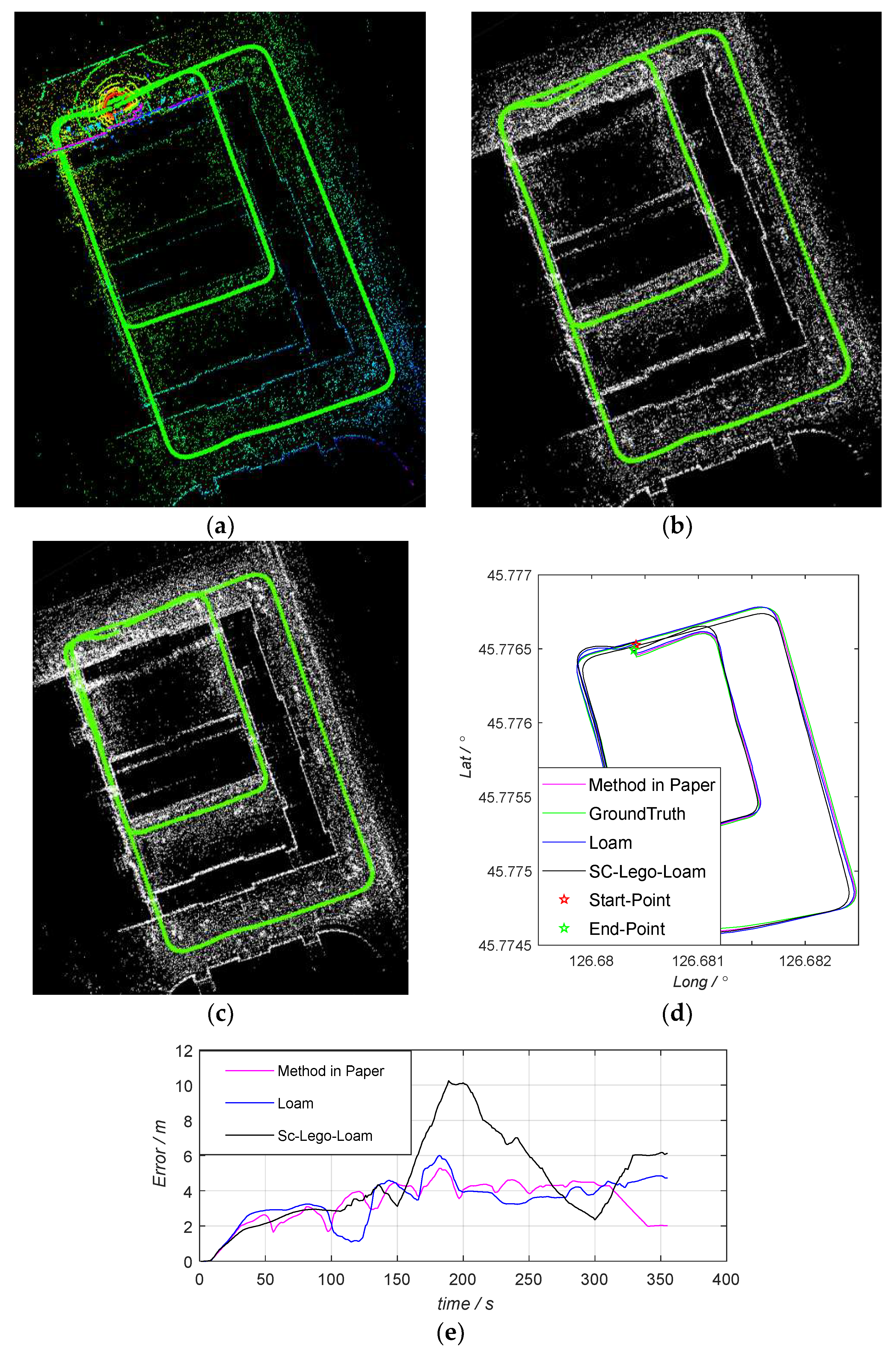
In conventional scenarios, the performance of the algorithm proposed herein was comparable to that of LOAM. However, in scenarios where structural features were sparse or lacking, the algorithm demonstrated superior performance. The experimental results indicate that, while the algorithm achieved results similar to LOAM under typical conditions, it excelled in environments with limited structural features. In experiments that satisfied loop closure conditions, its relative advantage was even more pronounced. The relative accuracy improved by approximately 17%. From
Figure 12, it can be observed that, in a general scenario, although the algorithm in the paper achieved good results, its basic performance was consistent with the other two algorithms. This scenario was only to verify the universal applicability of the algorithm in the paper, so there was no significant improvement in the specific comparative data.
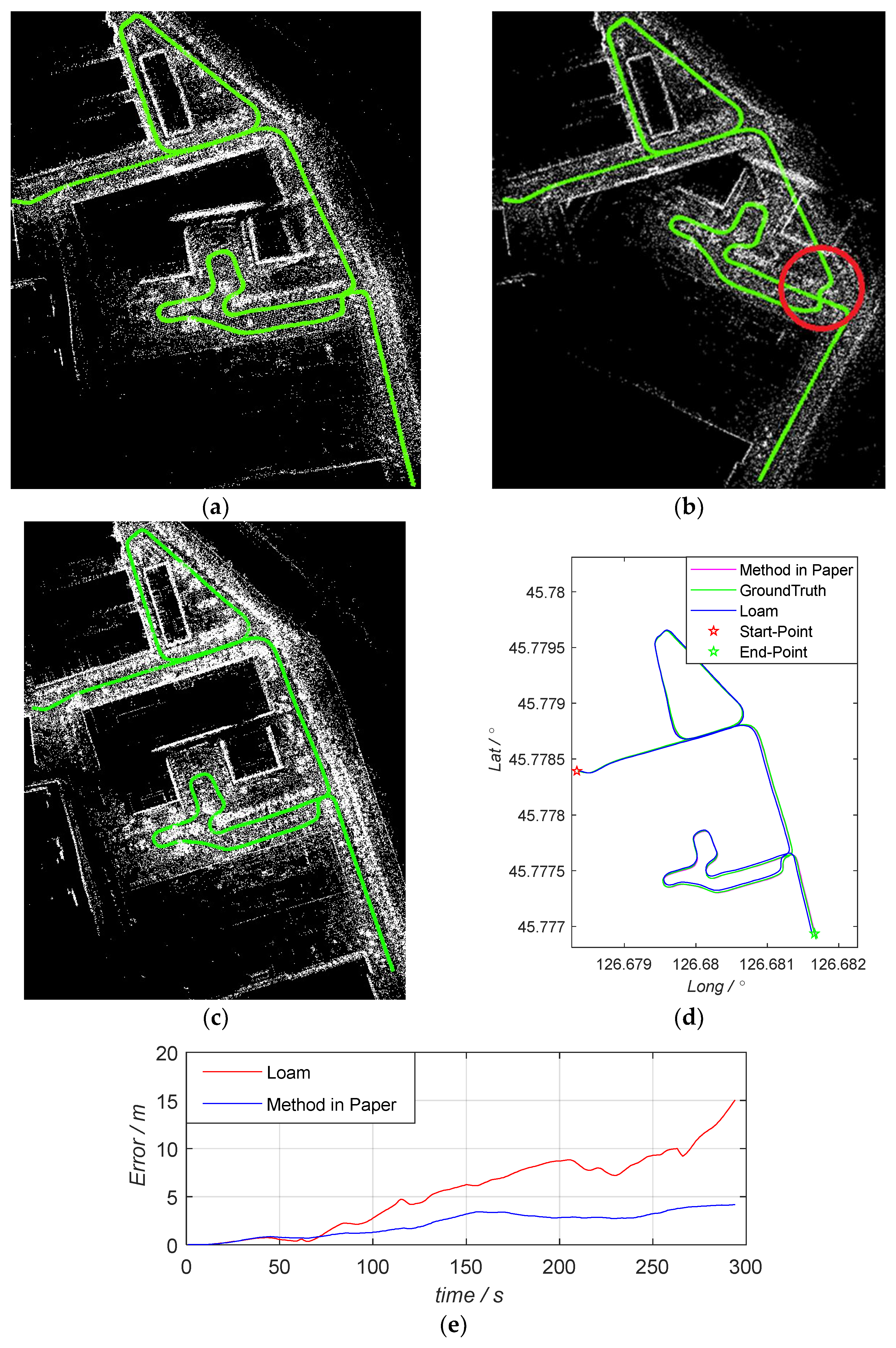
Figure 13 (DATA_2) is a preset scenario for the paper. Excluding the SC-Lego-LOAM algorithm, which was eliminated due to loop closure failure, from the error in
Figure 13e, it can be seen that, after entering the parking lot environment, the error of the LOAM algorithm began to gradually increase, while the algorithm in the paper maintained a stable trajectory tracking. This fully demonstrated that the algorithm proposed in the paper achieved optimization for special scenarios while maintaining universality.
At the same time, this paper reorganizes and extracts the inherent characteristics of the point cloud. It goes a step further in the use of points, focusing the application of LiDAR point clouds on the edges that are less susceptible to the sparsity of point clouds and frequent changes in attitude matrices. This virtual edge composed of edge points is inherently a form of clustering. As long as points that meet the clustering criteria can be scanned, they can be continuously tracked in LiDAR SLAM and used to correct the positioning results of SINS. Of course, considering that the density of the point cloud has an attenuation characteristic with distance, in actual selection, further screening will only be carried out when a cluster contains at least four consecutive points and the line length exceeds 1 m. The selection of line distance rather than points, lines, or surfaces as the observation variable effectively reduces the computational load of the filter and increases the feasibility of real-time computation on low-performance devices.
For LiDAR SLAM loop closure based on scan context, the paper also makes certain rules changes. Experiments have proven that it can effectively reduce the occurrence of incorrect loop closure points and thereby enhance the overall accuracy of SLAM.
Although LiDAR SLAM algorithms based on machine learning have achieved excellent results, for in-vehicle processors, due to limitations in size and power, it is still difficult for their core to meet the real-time requirements in navigation. This work provides another feasible path within traditional algorithms.
5.2. Further Research
The experimental results presented in this paper demonstrate that the algorithm proposed within the text has superiority over traditional algorithms in both the odometry and mapping components of LiDAR SLAM. However, the results for Data_5 also indicate that in complex long-distance environments, relying solely on LiDAR and SINS for navigation still cannot achieve long-term precise positioning. This suggests that the algorithm presented in the paper should only be used as a supplementary method to maintain the original navigation accuracy when GNSS signals are lost, rather than a complete substitute, in urban environments. In future research, exploring how to integrate GNSS-related data to further enhance the performance of LiDAR SLAM will be investigated.
Additionally, another point that requires attention is that, similar to other LiDAR algorithms, the divergence issue in the height channel of the algorithm presented in the paper has not been significantly improved. When the LiDAR is scanning in open areas (such as forest trails), it becomes extremely difficult to obtain lateral edge lines, and at this point, 3D LiDAR SLAM can degrade to a performance like that of 2D LiDAR SLAM. Furthermore, how to further subdivide and utilize ground points will also be one of the key research projects’ focuses in the future.
6. Conclusions
This paper presents a novel LiDAR/SINS tightly integrated SLAM algorithm designed to address the localization challenges in urban environments characterized by sparse structural features. Building upon the LOAM framework, the algorithm introduces further processing of LiDAR point cloud classification to extract edge lines through clustering. Leveraging the rotational invariance of distance, the algorithm constructs a Kalman filter system based on the distance variation in edge lines. This approach contributes to enhanced robustness and positioning accuracy.
Experimental results obtained in local urban scenarios demonstrated a 17% enhancement in positioning accuracy when compared to traditional point-based methods, particularly in environments characterized by sparse features. By proposing a line distance-based observation model and detailing the associated EKF framework and parameter settings, the proposed method redefines the concepts of loosely and tightly coupled integration within LiDAR/SINS systems.
Future research will explore the integration of GNSS data to further enhance the performance of the proposed LiDAR SLAM system, particularly in complex and long-distance navigation scenarios. Additionally, key areas of focus for future work include improving performance in open areas, particularly in the vertical channel, and optimizing ground point utilization.
This study not only achieves significant algorithmic improvements over existing methods but also paves a new technological pathway for autonomous driving and robotic navigation applications.
