Article

Random Stepped Frequency ISAR 2D Joint Imaging and Autofocusing by Using 2D-AFCIFSBL

School of Artificial Intelligence, Xidian University, Xi’an 710126, China
*
Author to whom correspondence should be addressed.
Remote Sens. 2024, 16(14), 2521; https://doi.org/10.3390/rs16142521
Submission received: 22 April 2024 / Revised: 14 June 2024 / Accepted: 3 July 2024 / Published: 9 July 2024
(This article belongs to the Topic Computational Intelligence in Remote Sensing: 2nd Edition)

Abstract

:
With the increasingly complex electromagnetic environment faced by radar, random stepped frequency (RSF) has garnered widespread attention owing to its remarkable Electronic Counter-Countermeasure (ECCM) characteristic, and it has been universally applied in inverse synthetic aperture radar (ISAR) in recent years. However, if the phase error induced by the translational motion of the target in RSF ISAR is not precisely compensated, the imaging result will be defocused. To address this challenge, a novel 2D method based on sparse Bayesian learning, denoted as 2D-autofocusing complex-value inverse-free SBL (2D-AFCIFSBL), is proposed to accomplish joint ISAR imaging and autofocusing for RSF ISAR. First of all, to integrate autofocusing into the ISAR imaging process, phase error estimation is incorporated into the imaging model. Then, we increase the speed of Bayesian inference by relaxing the evidence lower bound (ELBO) to avoid matrix inversion, and we further convert the iterative process into a matrix form to improve the computational efficiency. Finally, the 2D phase error is estimated through maximum likelihood estimation (MLE) in the image reconstruction iteration. Experimental results on both simulated and measured datasets have substantiated the effectiveness and computational efficiency of the proposed 2D joint imaging and autofocusing method.

1. Introduction

Inverse synthetic aperture radar (ISAR) [1] can achieve 2D high-resolution images of noncooperative moving targets in all-day and all-weather scenarios, which plays a significant role in both civil and military fields [2]. For traditional ISAR imaging, it is usually necessary to transmit a large bandwidth signal to achieve high resolution in the range direction. However, transmitting a large bandwidth signal is not only susceptible to interference but also puts tremendous pressure on the radar system hardware. To overcome these difficulties, random stepped frequency (RSF) radar was introduced into the field of ISAR imaging [3]. Because the carrier frequency of RSF radar jumps rapidly and randomly [4], making it unpredictable, RSF radar exhibits excellent Electronic Counter-Countermeasure (ECCM) characteristics in modern complex electromagnetic environments [5]. RSF ISAR can synthesize wideband signals by transmitting a large number of narrowband pulses in a burst, thereby achieving high range resolution. RSF radar significantly reduces the instantaneous bandwidth requirements and overall cost of the radar system. Therefore, continuing to study RSF ISAR imaging is valuable. However, RSF ISAR requires a long coherent processing interval (CPI), which invalidates the assumption of a constant rotation rate of the target and further affects the quality of imaging. To mitigate this issue, sparse RSF (SRSF) technology [6] has been introduced, reducing CPI by transmitting fewer subpulses and bursts. At the same time, random stepped frequency radar can track and image multiple targets, which can result in the loss of some pulses. Additionally, in complex electromagnetic environments, some subpulses and bursts may be unavailable, making the study of SRSF ISAR imaging highly significant.
Considering the inherent sparsity of radar observation targets in space, ISAR imaging can be seen as a problem of sparse signal reconstruction. Compressive sensing (CS) [7], capable of reconstructing sparse signals from insufficient measurements, has been widely applied in the ISAR imaging field in recent years. It has been demonstrated to be more effective than many other methods [8]. Similar to traditional range-Doppler (RD) methods, the most common methods based on CS synthesize high-resolution images separately for the range and cross-range directions [6,9]. Consequently, a number of CS-based reconstruction algorithms have been employed in RSF ISAR imaging, including orthogonal matching pursuit (OMP) [10], smoothed 0 norm (SL0) [11], 1 norm optimization [9] and alternating direction method of multipliers (ADMM) [12]. Nevertheless, the imaging quality of these algorithms relies on the choice of model parameters and is influenced by the SNR of the echo and sparse aperture. Unlike other methods that require manual parameter adjustment, the sparse Bayesian learning (SBL) [13] algorithm produces superior reconstruction outcomes without the need for manual parameter adjustment. Many ISAR imaging methods based on the SBL algorithm have been introduced [14,15,16,17]. However, these SBL algorithms typically involve matrix inversion with high computational complexity, resulting in the computational complexity of SBL-based ISAR imaging algorithms being impractical. Zhang et al. [18] proposed a sparse Bayesian algorithm based on ADMM, treating the problem of solving the posterior expectation of sparse vectors as a convex optimization problem. ADMM is utilized to solve this convex optimization problem, thus avoiding matrix inversion. While the complexity of the algorithm is reduced, it introduces manually adjusted regularization parameters.
However, the sequential imaging method does not fully account for the two-dimensional sparsity of ISAR images, resulting in a decrease in imaging quality. To enhance imaging sparsity, a joint imaging framework is proposed, which can acquire high-resolution profiles in both range and cross-range directions simultaneously. It is common practice to vectorize a 2D ISAR image [19,20]. However, vectorized optimization encounters challenges in terms of high computational complexity and substantial memory requirements due to the large dictionary dimension. To directly process sparse matrix data, various 2D compressive sensing (2D-CS) algorithms, including 2D smoothed 0 norm (2D-SL0) [21], 2D-FISTA [22], 2D-ADMM [12], have been proposed. Unlike the above iterative optimization algorithm, which requires an extensive manual adjustment of model parameters to achieve optimal results in experiments, the SBL-based method does not. However, many Bayesian algorithms struggle with directly handling two-dimensional sparse matrices and face challenges such as matrix inversion and high computational complexity. Zhang et al. [23] proposed a 2D-Fast SBL for ISAR joint imaging. However, this method requires converting the complex matrix into a real matrix, leading to increased computational complexity.
The relative motion of a target to the radar can generally be decomposed into two parts: translation and rotation [24]. Achieving high-resolution ISAR imaging requires precise compensation for the target’s translational motion. However, accurately estimating the motion parameters of the target can be challenging, particularly in SRSF ISAR scenarios with sparse subpulses and gapped apertures, which further affect algorithm performance. Huang et al. [3] introduced an RSF ISAR motion compensation and imaging method, approximating the target’s translational motion as uniform. However, this simplistic approximation leads to residual phase errors, making focusing challenging. An approach to mitigate this is integrating autofocusing into the ISAR image reconstruction process. Zhao et al. [25] used maximum likelihood estimation (MLE) criterion to estimate phase errors during ISAR imaging, reducing the phase error impact. Zhang et al. [26] used the minimum entropy criterion as the optimization goal for the autofocusing process, aiming to improve the quality of sparse aperture ISAR imaging. Li et al. [27] proposed a joint imaging and autofocuing method using MLE criterion to estimate the phase error and a 2D-ADMM method for ISAR imaging. The aforementioned algorithm can mitigate the influence of phase errors on the cross-range direction and produce a well-focused ISAR image. RSF radar synthesizes high-resolution profiles in the distance dimension through multi-pulse synthesis, so there is not only a phase error in the cross-range direction but also a phase error in the distance dimension, posing challenges for existing algorithms regarding effectively addressing range-dimensional defocus. Thus, Shao et al. [28] proposed a 2D joint ISAR imaging and motion compensation algorithm for sparse stepped frequency radar, addressing translation-induced phase errors. However, it cannot handle phase errors from model inaccuracies or system defects. To tackle this issue, Wang et al. [29] introduced imaging autofocusing and motion compensation algorithms. However, vectorizing ISAR images leads to an increased computational burden. Using the 2D-ADMM algorithm, Lv et al. [30] proposed 2D-IADIA to alternately obtain ISAR imaging and phase estimation. However, the quality of the imaging results is highly dependent on the selection of model regularization parameters. To avoid manual parameter tuning, Lv et al. [31] further unfolded 2D-IADIA into a deep neural network, which has better robustness than traditional algorithms.
In this paper, we propose a 2D joint imaging and autofocusing method named 2D-autofocusing and complex-value inverse-free SBL (2D-AFCIFSBL) for SRSF ISAR, aiming to achieve high-resolution imaging from 2D sparse received data. To begin, to leverage the full potential of 2D coupling information of echoes, we develop a vectorized representation model that integrates high-resolution ISAR imaging and 2D phase error estimation. After that, the probabilistic modeling is performed on the ISAR image, which has a gamma-complex Gaussian hierarchical imposed prior to ensure the sparsity of the model, and then variational Bayesian inference is used for image reconstruction in the complex domain. Due to the enormous computational complexity caused by matrix inversion at each iteration in Bayesian inference, matrix inversion is avoided by relaxing the evidence lower bound function (ELBO), which transforms the covariance matrix to be inverted into a diagonal matrix. So as to accomplish phase autofocusing during the ISAR image reconstruction process, the 2D phase error is estimated through MLE in the image reconstruction iteration. To further alleviate the storage pressure and improve the imaging efficiency, the iterative process is reformulated into a matrix form by leveraging the properties of the Kronecker product. Finally, both simulated and measured dataset experiments demonstrate that the proposed 2D joint method has excellent performance and efficiency compared to other joint imaging and autofocusing methods.
The remainder of this article is organized as follows. Section 2 formulates a 2D imaging model incorporating a 2D phase error for SRSF ISAR. Section 3 proposes the joint imaging and autofocusing probabilistic model and provides a detailed derivation and discussion of the 2D-AFCIFSBL method for solving this model. Section 4 evaluates the performance of the proposed method by simulated and measured datasets compared to the 2D-Fast SBL, 2D-IADIA and 2D-UADN methods. Section 5 concludes this article and discusses future work. Unless specifically defined, the following mathematical symbols will be used in this article. The bold letters denote matrices or vectors. Given a matrix A , A i · , A · j , A i j , A 1 , A * , A T and A H represent the ith row, jth column, ( i , j ) th entry, inverse, conjugate, transpose, and conjugate transpose of A , respectively. ⊗, ⊙ and ⊘ represent the Kronecker, Hadamard products and element-wise division, respectively. R and C denotes the real and complex domains, respectively.

2. Imaging Model for RSF ISAR

The RSF ISAR system transmits N subpulses in a burst to acquire high resolution in the range direction, and it transmits N a bursts in a CPI to acquire high resolution in the cross-range direction. Assuming n = [ 0 , 1 , , N 1 ] and n a = [ 0 , 1 , , N a 1 ] , we can express the nth subpulse in the n a th burst of the transmitted signal as follows
s t ( t , n , n a ) = rect t n a N T r n T r T p exp [ j 2 π f n ( t N a N T r n T r ) ]
where T r , T p , and f n denote the subpulses repetition interval, the subpulses bandwidth and the carrier frequency of the nth subpulse, respectively. Random step frequency signals show stronger anti-interference characteristics compared to traditional step frequency signals, which is primarily due to the random frequency hopping step size. Here, the carrier frequency of the nth subpulse is given by f n = f c + Γ ( n ) Δ f , where f c is the initial carrier frequency, Γ ( n ) is the nth randomized modulation code chosen from the set of [ 0 , 1 , 2 , , N 1 ] , and Δ f is the stepped frequency. Moreover, Δ f is defined as Δ f = 1 / T p , resulting in the synthetic bandwidth B = N Δ f . rect ( · ) is the rectangular function denoted as
rect ( t ) = 1 0 t 1 0 otherwise
Figure 1 shows the ISAR imaging turntable model. We assume that the electromagnetic scattering characteristics of the target can be modeled as the superposition of K strong scattering centers. Then, the received echo signal can be denoted as
s r ( t ^ , n , n a ) = k = 1 K σ k rect t ^ 2 R k ( t ) / c T p exp [ j 2 π f n ( t ^ 2 R k ( t ) / c ) ]
where t ^ = t n a N T r n T r is fast time and σ k denotes the scattering coefficient of the kth strong scattering center. R k ( t ) denotes the instantaneous distance between the kth strong scattering center and the radar at time t.
Based on the “stop-and-go” assumption, it holds that R k ( t ) R k ( t n , n a ) , where t n , n a = n a N T r + n T r . And  R k ( t n , n a ) can be deduced as follows
R k ( t n , n a ) = R O ( t n , n a ) + x k sin ( ω t n , n a ) y k cos ( ω t n , n a )
where R O ( t n , n a ) r 0 + v t t n , n a + a / 2 t t n , n a 2 is the instantaneous radar distance of the specific point O at time t n , n a , which represents the translational motion of the target. And  r 0 , v, a is the initial range between radar and the point O, the speed of the target and the acceleration of the target, respectively. x k sin ( ω t n , n a ) + y k cos ( ω t n , n a ) denotes the rotational motion of the kth scatter, while ( x k , y k ) is the coordinate of the kth scattering point on the imaging plane. ω represents the angular speed. Due to the assumption of a short CPI, the equivalent rotation angle during the CPI is not very large. Therefore, Equation (4) can be expanded using a Taylor series and neglecting terms of the second order and higher, leading to
R k ( t n , n a ) R O ( t n , n a ) + x k ω t n , n a y k
Before imaging, compensating for translational motion is necessary. However, traditional motion compensation methods suffer from low accuracy due to the downsampling of the echo signal [32]. The random selection of subpulse carrier frequencies poses a challenge in accurately estimating the parameters of translational motion using parametric methods. Since the translational motion parameters of the target cannot be accurately estimated, there will still be residual phase error after translation compensation. Therefore, the sampled echo neglecting the constant term can be denoted as
s r ( n , n a ) exp ( j ϕ ( n , n a ) ) k = 1 K σ k exp [ j 4 π Γ ( n ) Δ f y k c ] exp [ j 4 π f c x k ω n a N T r c ]
where ϕ ( n , n a ) consists of two parts: the phase residual after translation motion compensation and the model error [29]. It can be expressed as
ϕ ( n , n a ) = 4 π f n ( ( v v ^ ) t n , n a + ( a a ^ ) t n , n a 2 / 2 ) c + Δ ϕ ( n , n a )
where v ^ , a ^ denote the estimated speed of acceleration of the target, and  Δ ϕ ( n , n a ) represents the model error.
The SRSF echo signal matrix is obtained by random sampling from the RSF echo signal matrix. Assume the SRSF echo signal contains H ( H N a ) bursts and M ( M N ) subpulses in each burst, and the echo signal data matrix S C M × H can be written as
S = Φ r E Φ a T Φ r F r X F a T Φ a T + G = E F r X F a T + G
where E C N × N a , X C P × Q , G C M × H represent the phase error matrix, the 2D ISAR image and the noise matrix, respectively. Among them, S and E can be denoted as
S = s r ( 1 , 1 ) s r ( 1 , 2 ) s r ( 1 , H ) s r ( 2 , 1 ) s r ( 2 , 2 ) s r ( 2 , H ) s r ( M , 1 ) s r ( M , 2 ) s r ( M , H ) M × H
E = e ( 1 , 1 ) e ( 1 , 2 ) e ( 1 , N a ) e ( 2 , 1 ) e ( 2 , 2 ) e ( 2 , N a ) e ( N , 1 ) e ( N , 2 ) e ( N , N a ) N × N a
where e ( 2 , 2 ) = exp ( j ϕ ( n , n a ) ) . F r C N × P ( N P ) and F a C N a × Q ( N a Q ) denote the range and the cross-range sensing matrix, respectively, which can be written as
F r = f r ( 1 , 1 ) f r ( 1 , 2 ) f r ( 1 , P ) f r ( 2 , 1 ) f r ( 2 , 2 ) f r ( 2 , P ) f r ( N , 1 ) f r ( N , 2 ) f r ( N , P ) N × P
F a = f a ( 1 , 1 ) f a ( 1 , 2 ) f a ( 1 , Q ) f a ( 2 , 1 ) f a ( 2 , 2 ) f a ( 2 , Q ) f a ( N a , 1 ) f a ( N a , 2 ) f a ( N a , Q ) N a × Q
where f r ( n , p ) = exp ( j 2 π Γ ( n ) p 1 P ) and f a ( n a , q ) = exp ( j 2 π n a q 1 Q ) . Φ r R M × N and Φ a R H × N a represent the randomly downsampling matrices, which can be acquired by randomly selecting M and H rows of two identity matrices with sizes of N × N and N a × N a , respectively. F a = F a Φ a and F r = Φ r F r . E = Φ r E Φ a T represent the two-dimensional phase error matrix after downsampling.
Due to the impact of the two-dimensional phase error E , several 2D reconstruction algorithms like 2D-SL0 and 2D-FISTA, as well as algorithms that only consider one-dimensional phase error such as 2D-UADN [27], struggle to effectively reconstruct ISAR images. Although the 2D-IADIA [30] algorithm, which accounts for two-dimensional phase errors, can reconstruct ISAR images, it is difficult to adjust the regularization coefficient. While the SBL algorithm does not require manual parameter adjustment, most current SBL algorithms are not directly applicable to matrix solving and have high computational complexity. A straightforward approach involves using the Kronecker product [33] to transform the 2D ISAR model from Equation (8) into a one-dimensional model, representing it in an equivalent vector form, and subsequently applying Bayesian algorithms for reconstruction. Then, to improve computational efficiency and alleviate storage pressure, the vectorized iteration is transformed into matrix iteration. Taking into account the effect of the two-dimensional phase error E , the vectorized equivalent model of Equation (8) can be formulated as follows
s = e ( F a F r ) x + g = e f x + g
where s = vec ( S ) C M H × 1 , x = vec ( X ) C P Q × 1 , g = vec ( G ) C M H × 1 . The dictionary matrix f = F a F r C M H × P Q , vec ( · ) denotes the vectorization operation. e C M H × M H is a diagonal matrix, which can be denoted as
e = diag e j ϕ 1 , 1 , , e j ϕ M , 1 , e j ϕ 1 , 2 , , e j ϕ M , H = e j ϕ 1 , 1 0 0 0 e j ϕ 2 , 1 0 0 0 e j ϕ M , H M H × M H
where diag ( · ) is an operation creating a diagonal matrix using the elements inside.

3. Proposed 2D-AFCIFSBL Method

In this section, we first derive the 1D complex inverse-free SBL algorithm based on the model (13). To improve computational efficiency, the properties of the Kronecker product are then used to transform the iterative process into a matrix form. Finally, two-dimensional self-focusing is integrated into the imaging process to develop the 2D-AFCIFSBL algorithm.

3.1. ISAR Imaging Based on Variational Bayesian Inference

In this section, a probabilistic model is established for the ISAR imaging shown in (13), and then variational Bayesian inference is used for image reconstruction.
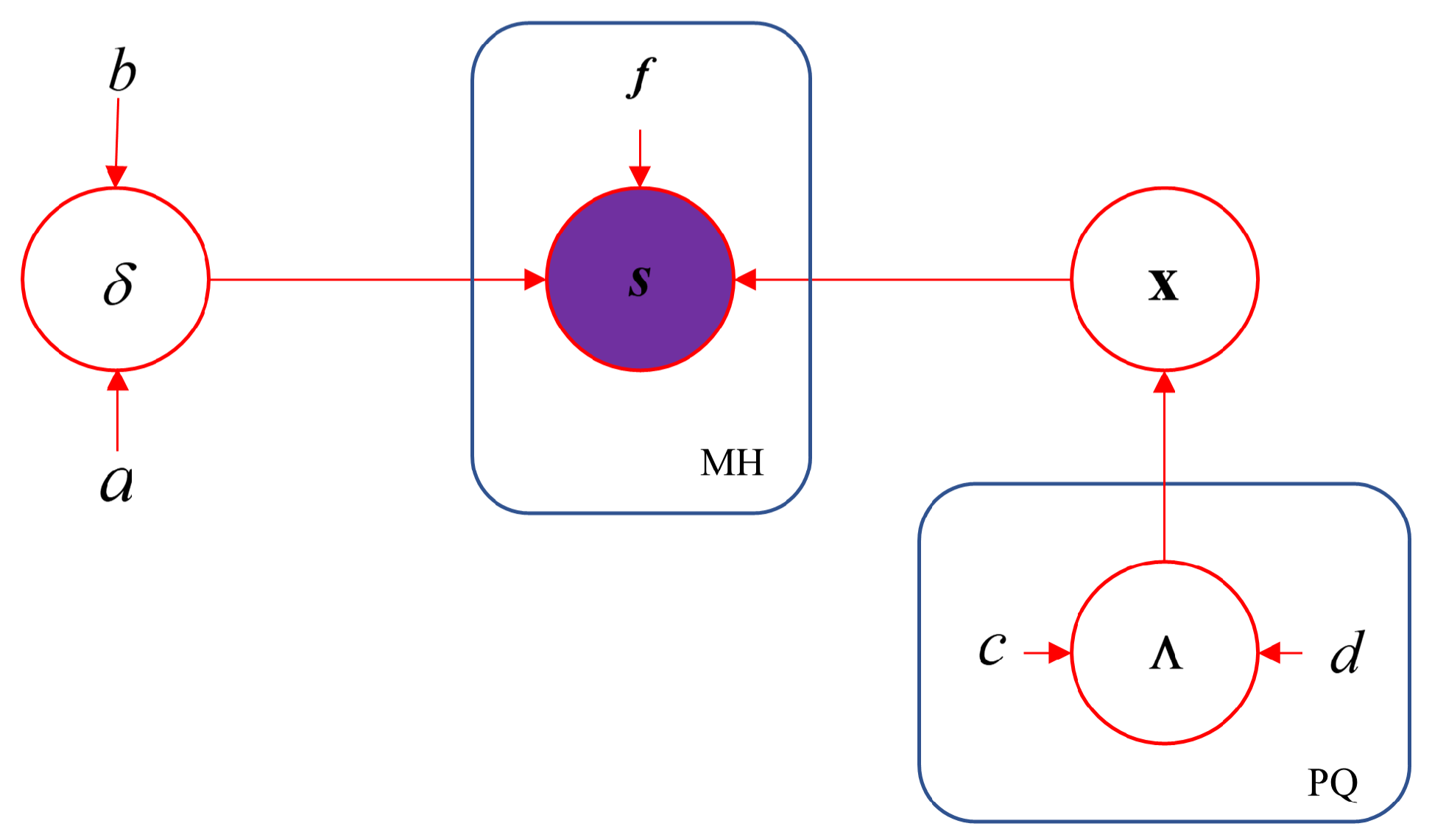
In the SBL framework, we usually assume that the noise follows zero-mean complex Gaussian distribution CN ( g | 0 , δ 1 I ) , where CN ( · ) denotes complex Gaussian distribution and δ is the reciprocal of the noise variance. Therefore, the likelihood function of the received echo signal s can be written as
p ( s ) = CN ( s | e f x , δ 1 I M H )
where I M H is the identity matrix with size M H × M H . δ has a gamma distribution applied
p ( δ ) = G a m m a ( δ | a , b )
where G a m m a ( · ) denotes gamma distribution, and a, b are the position and scale parameter, respectively. To promote the sparsity of the ISAR image, we impose a hierarchical Bayesian prior on x . In the first layer, a distinctively Gaussian distribution is placed on each pixel of the sparse vector x
p ( x ) = CN ( x | 0 , α )
where α = diag ( α 1 1 , α 2 1 , , α P Q 1 ) . α i 1 denotes the variance of x i . α i and x i are the ith element of α and x . In the second layer, we impose Gamma distribution with position parameter c and scale parameter d on the reciprocal of the variance α i
p ( α ) = i P Q G a m m a ( α i | c , d )
Finally, the corresponding probabilistic graphical model is illustrated in Figure 2. Our aim is to estimate the posterior of all latent variables θ = { x , α , δ } , whose posterior can be computed through the variational Bayesian inference algorithm [34]. In the traditional VB method, the evidence lower bound (ELBO) is expressed by
ELBO q = θ q θ log p s , x , α , δ q θ
where p s , x , α , δ = p ( s | x , δ ) p ( x | α ) p ( α ) p ( δ ) , q θ = q x ( x ) q α ( α ) q σ ( σ ) .
To speed up computation, we employed relaxed-ELBO as a replacement for the ELBO, which eliminates the need to invert a matrix [35]. Assume f is a Lipschitz continuous function, so there exists a number T f ( x ) 2 , x such that for any u , v , we have:
f ( u ) f ( v ) + ( u v ) H f ( v ) + ( u v ) H T ( u v )
Then, the lower bound on p ( s | x , δ ) can be obtained as
p ( s | x , δ ) = δ P Q π P Q exp δ 2 s e f x 2 2 G ( s , x , δ ; z )
where G ( s , x , δ ; z ) is defined as
G ( s , x , δ ; z ) = δ P Q π P Q exp 2 δ ( x z ) H f H f z f H e H s δ s e f z 2 2 T 2 δ x z 2 2
where ( · ) denotes taking the real parts and T is slightly larger than the eigenvalue of matrix 2 f H f . When x = z , the inequality becomes an equality. Then, the relaxed-ELBO can be written as
relaxed ELBO q , z = θ q θ log F s , θ , z q θ
where F s , θ , z = G ( s , x , δ ; z ) p ( x | α ) p ( α ) p ( δ ) and θ = { x , α , δ } is the latent variable to be estimated. In the VBE-step, z is held fixed, and Equation (24) is used iteratively to approximately compute the posterior probability density function for each latent variable.
ln q θ i ( θ i ) = ln F ( s , θ , z ) q j i + const
Then, the posterior of x can be regarded a complex Gaussian distribution
q x ( x ) = CN ( x | μ , Σ )
μ = δ Σ T z 2 + f H e H s f H f z
Σ = T δ 2 I + D 1
where D = diag ( α 1 , α 2 , , α P Q ) and · denotes the exception operation. It can be seen that the covariance matrix Σ is a diagonal matrix. The calculation of Equation (27) does not require the inversion operation of the matrix. Therefore, the computational efficiency is significantly improved compared to the traditional Bayesian algorithm.
For noise precision δ , the approximate posterior q δ ( δ ) is the Gamma distribution, which can be written as
q δ ( δ ) = G a m m a ( δ | a ˜ , b ˜ )
a ˜ = a + M H
b ˜ = b + g ( x , z )
with
g ( x , z ) = s e f z 2 2 + 2 ( x z ) H f H f z f H e H s + T ( μ z 2 2 + t r ( Σ ) ) / 2
Thus, δ can be expressed as the expectation of δ
δ = a ˜ b ˜
The approximate posterior of α is the distinctively Gamma distribution, which can be written as
q α ( α ) = i = 1 P Q G a m m a ( α i | c ˜ , d i ˜ )
c ˜ = c + 1
d ˜ i = d + x i * x i
where x i * x i = x i * x i + | Σ i , i | . Σ i , i denotes the ith element on the diagonal of matrix Σ . Thus, α can be expressed as the expectation of α
α i = c ˜ d i ˜
In the VBM step, the approximate posterior q ( θ ) remains fixed.
z n e w = arg max z ln F ( s , θ , z ) q ( θ ; z o l d ) = Q ( z | z o l d )
By differentiating Equation (37) and setting it equal to zero, we can find the value of  z n e w .
Q ( z | z o l d ) z = ( T I P Q 2 f H f ) ( z μ ) = 0
Since T is slightly larger than the maximum eigenvalues of matrix 2 f H f , T I P Q 2 f H f is a positive-definite matrix. Therefore, we can obtain the value of z n e w as
z n e w = μ
By alternately and iteratively executing the VBE step and VBM step, the vectorized ISAR image x = μ is finally obtained. Although the above process of reconstructing the sparse vector x avoids calculating the inverse of the matrix Σ , converting the 2D echo and ISAR images into vectors imposes significant computational and storage burdens. As the dimensions N, N a , P, and Q increase, the observation matrix f also rapidly expands, leading to computational challenges. In contrast, matrix operations offer higher computational efficiency and require less storage space than vectorized calculations. Therefore, it is necessary to convert the above calculation process into matrix operations to efficiently address the matrix sparse problem. Assuming μ = vec ( U ) , z = vec ( Z ) , we can rewrite the third part of Equation (26) as
f H e H s f H f z = ( F a F r ) H e H s ( F a F r ) H ( F a F r ) z = ( F a H F r H ) e H s ( F a H F a ) ( F r H F r ) z = vec F r H E * S F r Z F a T F a *
Then, Equations (26) and (27) can be expressed as the matrix form
U = δ T Z 2 + F r H E * S F r Z F a T F a * Σ P × Q
Σ P × Q = 1 P × Q ( T δ 2 1 P × Q + D P × Q )
where Σ P × Q = ( Σ ) , D P × Q = ( D ) . represent the extraction of the diagonal elements of matrix Σ to form a matrix of size P × Q . 1 P × Q is a matrix with all elements equal to 1, and its size is P × Q . T = 2 λ m a x ( F r H F r ) · λ m a x ( F a H F a ) + 10 5 is slightly larger than the Lipschitz constant. λ m a x ( · ) denotes the extraction of the maximum eigenvalue of a matrix.
We can rewrite Equations (32) and (36) in matrix form
δ = a + M H b + g ( X , Z )
D P × Q = ( c + 1 ) ( d + U U * + | Σ P × Q | )
where g ( X , Z ) can be rewritten in matrix form
g ( X , Z ) = S E F r Z F a T F 2 + 2 · sum ( U Z ) * F r H ( F r Z F a T E * S ) F a * + U Z F 2 + sum ( Σ P × Q ) 2 T
The second part of (45) can be obtained from the second part of (31)
2 ( x z ) H f H f z f H e H s = 2 vec U Z H ( F a F r ) H ( F a F r ) z e H s = 2 vec U Z H vec F r H ( F r Z F a T E * S ) F a * = 2 · sum ( U Z ) * F r H ( F r Z F a T E * S ) F a *
where · F represents the Frobenius norm and sum ( · ) denotes the summation of matrix elements. And Equation (39) can rewritten as
Z n e w = U
In the above derivation, while we assume the phase error matrix E is known, it is, in fact, unknown. Therefore, it becomes necessary to estimate the phase error during ISAR imaging.

3.2. Autofocusing Based on MLE

In this subsection, we estimate the two-dimension phase error matrix E through MLE in the image reconstruction iteration. Assuming that the ISAR image is known during the autofocusing process, the maximum likelihood estimation (MLE) problem can be converted into the following unconstrained optimization problem
e ^ = arg min e s e f x 2 2
For the lth iteration, the aforementioned Equation (48) can be transformed into an optimized form as follows
arg min E m = 1 M h = 1 H S m , h e j ϕ m , h F r X ( l ) F a T · , h m , · 2 2
where X ( l ) denotes the imaging result of the lth iteration. We initially decompose Equation (49) into the following minimization problem form
e ^ l + 1 m , h = arg min E S m , h e j ϕ m , h F r X ( l ) F a T · , h m , · 2 2
where e ^ l + 1 m , h represents the estimated phase error of the mth subpulse in the hth burst. Therefore, the optimal solution can be obtained by setting the first derivative of Equation (50) to zero
e ^ l + 1 m , h S m , h e j ϕ m , h F r X ( l ) F a T · , h m , · 2 2 = 0 e ^ l + 1 m , h = exp j · angle S m , h · F r X ( l ) F a T m , h *
where angle ( · ) is the operator of acquiring the phase information. To reduce memory requirements and improve computational efficiency, the estimation of the 2D phase error matrix can be further denoted in the matrix form
E ( l ) = exp j · angle S F r X ( l ) F a T *
In summary, detailed information on the proposed 2D fast ISAR imaging and autofocusing method has been presented in Algorithm 1.
Algorithm 1 2D-AFCIFSBL method
Input:  S C M × H
Output:  E , X
  1:
Initialization: δ ( 0 ) 1 , D P × Q ( 0 ) 1 P × Q , E ( 0 ) 1 P × Q , X ( 0 ) F r H S F a *
  2:
for  l = 1 , 2 , 3 , , L m a x  do
  3:
   Update X ( l ) by X ( l ) U using (41), (42)
  4:
   Update D P × Q ( l ) using (44)
  5:
   Update δ ( l ) using (43)
  6:
   Update Z ( l ) using (47)
  7:
   Update E ( l ) using (52)
  8:
   if  X ( l ) X ( l 1 ) F 2 / X ( l 1 ) F 2 10 4  then
  9:
      break
10:
   end if
11:
end for  X = X ( l ) , E = E ( l )
Here, L m a x is the maximum number of iterations of the algorithm. Finally, we provide a brief analysis of the complexity of the proposed 2D-AFCIFSBL algorithm. The complexity of each iteration of the 2D-AFCIFSBL algorithm mainly comes from the update of latent variables. For updating X and δ by (41), (42), (32), and (45), the computational complexity, which are O ( P Q ( M + H + 1 ) + M H ( P + Q + 1 ) ) and O ( P Q ( M + 2 H + 2 ) + M H ( 2 P + Q + 3 ) ) , respectively, mainly come from four matrix multiplications, element-wise multiplication and element-wise division. The update process for the 2D phase error matrix E by Equation (52), which has a computational complexity of O ( P Q H + M H ( P + 1 ) ) , primarily involves three matrix multiplications. Then, assuming P = Q and M , H < P , the worst case complexity of 2D-AFCIFSBL is O ( L m a x ( P 2 ( 2 M + 4 H + 2 ) ) .

4. Experiments and Analysis

In this section, we verified the effectiveness of the proposed RSF-ISAR imaging algorithm through simulated and measured datasets. Sparse data are obtained by randomly sampling in the range direction and the cross-range direction, respectively. The 2D SPR [30] is defined as γ = ( M / N , H / N a ) . For comparison, the 2D-Fast SBL method [23], 2D-UADN method [27] and 2D-IADIA method [30] are also adopted. For P = Q and M , N < P , the worst case complexity of 2D-Fast SBL, 2D-UADN and 2D-IADIA is O ( L m a x ( 4 P 2 ( 4 M + 4 H + 1 ) ) ) , O ( L m a x ( P 2 ( 2 M + 2 H + 1 ) ) and O ( L m a x ( P 2 ( M + 2 H ) ) ) , respectively, where L m a x is the maximum number of iterations. In addition, we utilized the image entropy (IE) [36] and target-to-background ratio (TBR) [37] to evaluate the imaging performance of different algorithms. For a well-focused image, the lower IE and the higher TBR values are expected. All experiments were conducted on a computer with an Inter Core i9-10900K CPU and 32GB RAM.

4.1. Experimental Results on Simulated Dataset

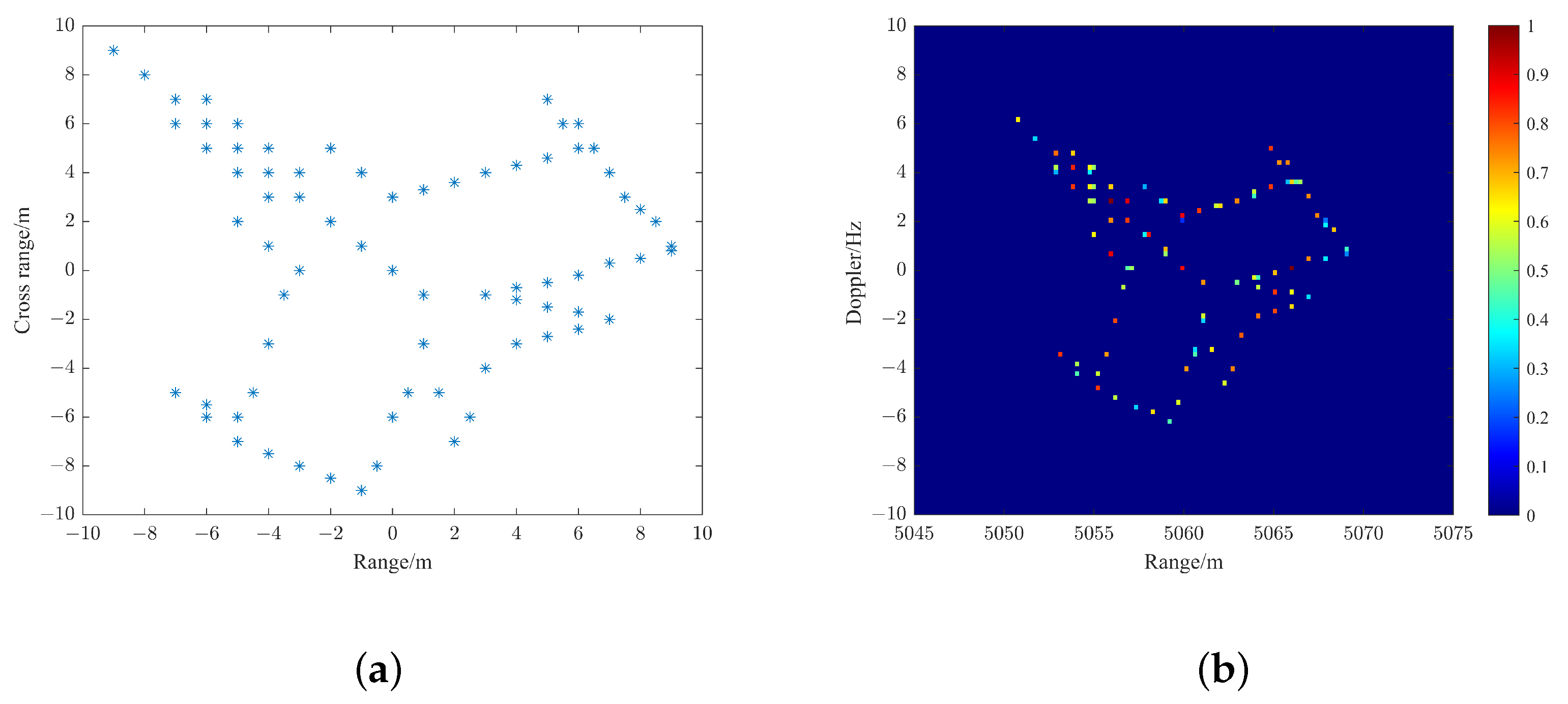
We preliminarily validated the imaging performance of the proposed 2D-AFCIFSBL algorithm by using the simulated dataset. The simulated dataset is generated by an X-band RSF radar with 10 GHz initial carrier frequency and 640 MHz bandwidth, and its main parameters are presented in Table 1. The target model in the simulated dataset consists of 74 independent scattering points presented in Figure 3a and its ISAR imaging result by using the 2D-AFCIFSBL method with complete echo data and no phase error added, as illustrated in Figure 3b. It is evident from the ISAR imaging result that the range between the target and the radar is 5060 m.
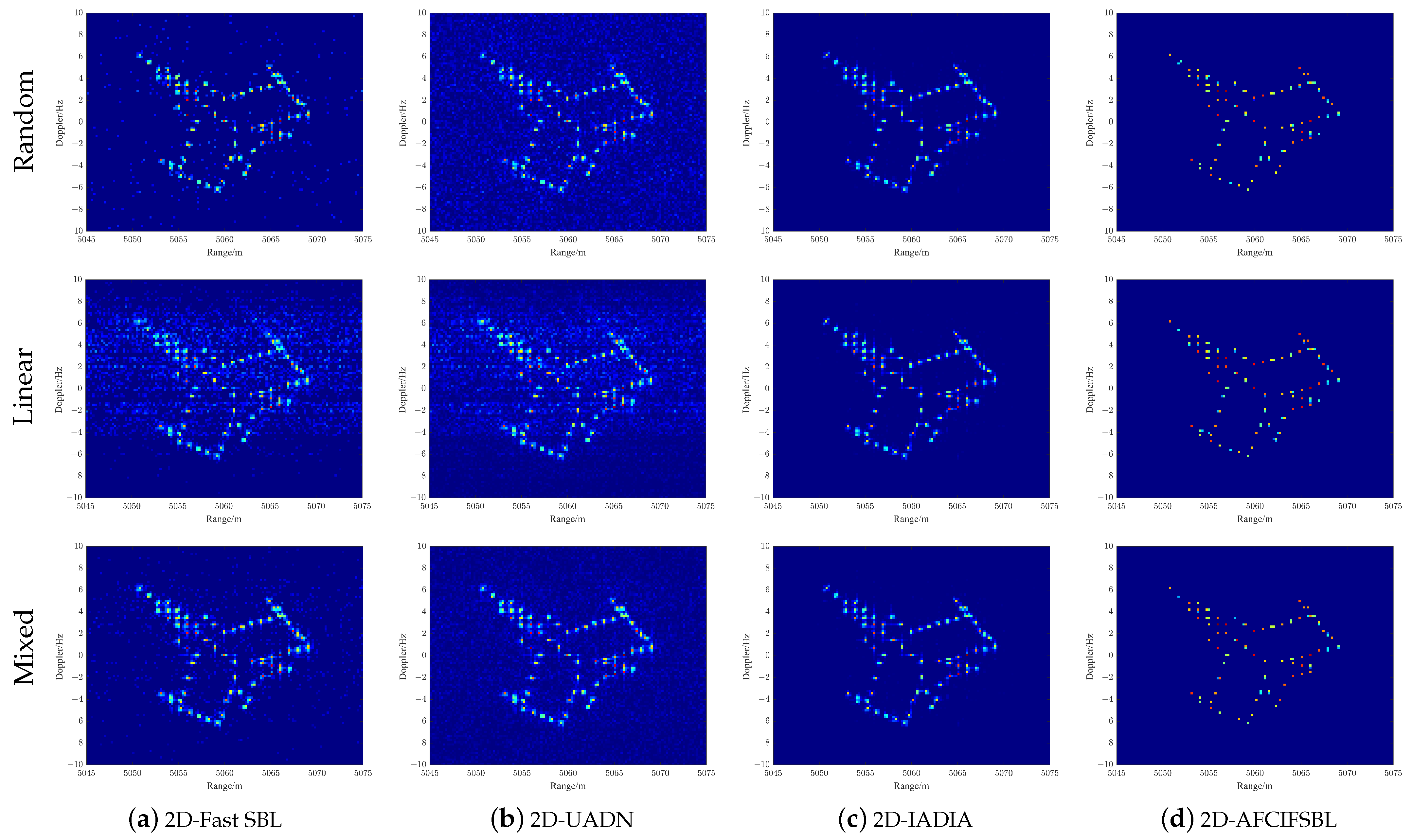
In the following experiments, we will add three types of 2D phase errors, namely random, linear and mixed phase errors to the raw simulation data separately as illustrated in Figure 4, to compare the phase error estimation capabilities of four methods. Among the three types of 2D phase errors, the amplitude variance of the random phase error is π / 2 , the linear phase error varies linearly between π / 2 and π / 2 and the mixed phase error is the mean of the random phase error and linear phase error. Additionally, we set the SNR of the experiment to 20 dB by adding complex-valued Gaussian noise into the raw simulated data.
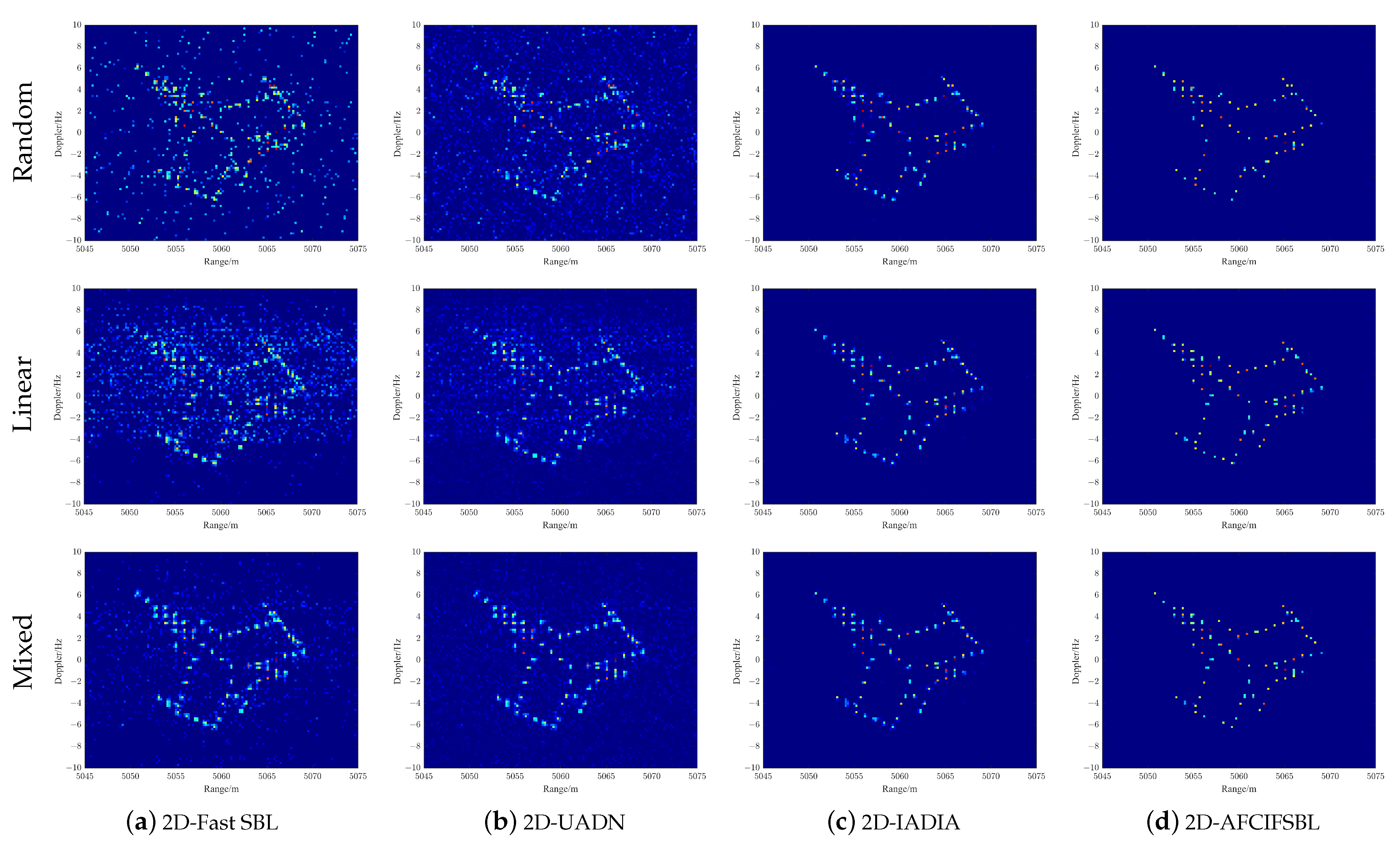
The first experiment is conducted under the ( 0.8 , 0.8 ) SPR and the imaging results acquired by aforementioned four methods, as illustrated in Figure 5. From the first column, it is evident that the imaging results produced by 2D-Fast SBL are contaminated by a large number of pseudo-scatterers under linear phase error. This limitation stems from the 2D-Fast SBL method’s incapacity to estimate and compensate for linear phase error. However, the imaging effect under random phase error is better than that under linear phase error because the random phase error can be regarded as random noise, and the SBL-based method can utilize prior sparsity to denoise. For the 2D-UADN method, it can estimate the phase error in the cross-range direction but does not account for the phase error in the range direction. Consequently, the resulting images acquired by the 2D-UADN method still have some pseudo-scatterers and noise floor under the linear phase error. In contrast, the proposed 2D-AFCIFSBL method consistently produces neat and well-focused images under all given types of phase errors, which verifies its robustness against phase errors. Particularly under the linear phase error condition, the imaging results acquired by using the 2D-Fast SBL method and 2D-UADN method exhibit significant noise floor, while the proposed 2D-AFCIFSBL method still achieves excellent results, implying its superior performance relative to other methods. In addition, through comparison of the third and fourth columns of images, it is evident that the 2D-IADIA and 2D-AFCIFSBL methods yield similar imaging results. But the 2D-AFCIFSBL method has lower image entropy than the 2D-IADIA method, as demonstrated in Figure 6. It is evident that due to the lack of 2D phase errors estimation, the image entropy of the 2D-Fast SBL method and 2D-UADN method is extremely high, especially in the condition of linear phase errors.
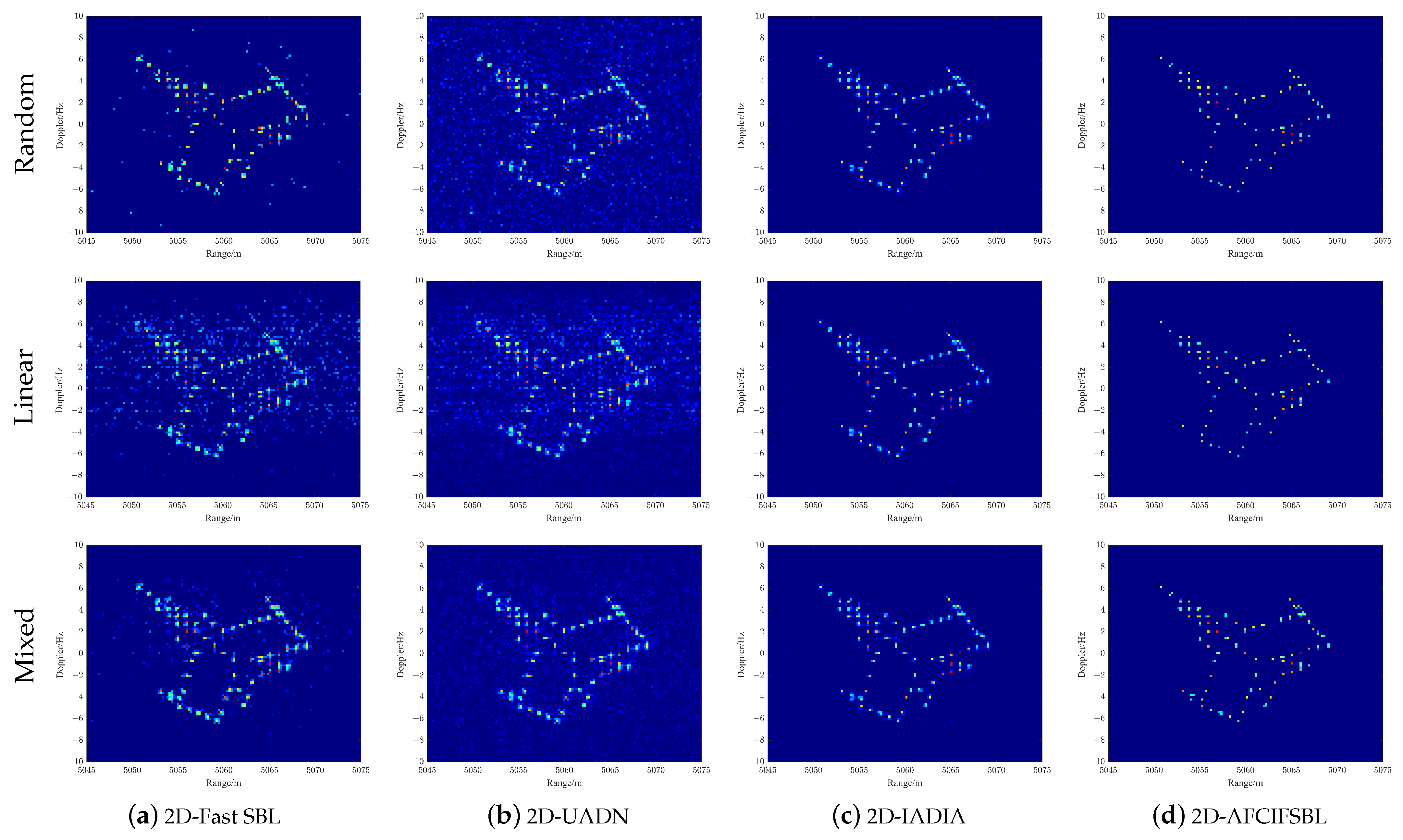
Figure 7 and Figure 8 show the imaging results under ( 0.6 , 0.6 ) and ( 0.4 , 0.4 ) SPR, and the corresponding image entropy of each SPR is presented in Figure 9 and Figure 10, respectively. It is evident from the image entropy curves that the four methods exhibit rapid convergence to a stable image entropy value. In particular, the 2D-UADN and 2D-Fast SBL methods acquire the highest image entropy under the random phase error and linear phase error, respectively, while the 2D-Fast SBL method has similar levels of image entropy to the 2D-UADN method under the mixed phase error. The imaging results in the first and second rows of Figure 7 and Figure 8 also demonstrate that under the linear phase error, the 2D-UADN method has slightly better imaging results than the 2D-Fast SBL method due to its 1D phase error estimation capability, while the 2D-Fast SBL method lacks any phase estimation. But the imaging results of the 2D-Fast SBL method and 2D-UADN method are both poor under all SPRs compared to the 2D-IADIA method and 2D-AFCIFSBL method. Upon comparing the imaging results between the 2D-IADIA and 2D-AFCIFSBL methods, it is evident that the image quality achieved by the 2D-IADIA method is comparable to that of the 2D-AFCIFSBL method. Only when the SPR is down to ( 0.4 , 0.4 ) do both methods begin to have few pseudo-scatterers and noise floor, but the phase error estimation ability of the 2D-IADIA method decreases more obviously. Additionally, the convergence speed of the 2D-IADIA method notably decreases at the SPR of ( 0.4 , 0.4 ) , while the 2D-AFCIFSBL method remains relatively stable, as shown in Figure 10. Therefore, the aforementioned experiments further substantiate the excellent imaging performance of the proposed 2D-AFCIFSBL method under three types of phase error with different SPR.
Subsequently, we assessed the imaging performance of the aforementioned four methods under different SNR conditions and only compared the imaging results under the random phase error, where the variance of the amplitude is π / 2 . Additionally, the SPR was set to ( 0.5 , 0.5 ) , which means that 128 subpulses and 128 bursts were randomly sampled from the complete echo data. The imaging results obtained by the four methods are demonstrated in Figure 11, in which the three rows from top to bottom represent the imaging results at 10 dB, 5 dB, and 0 dB, respectively. It is evident from the results that the proposed 2D-AFCIFSBL method obtains the lowest image entropy under all the given SNRs shown in Figure 12. Although the 2D-UADN method possesses the capability to estimate the 1D phase error in the cross-range direction, its imaging performance is adversely impacted by the 2D random phase error [27]. This results in an increase in pseudo-scatterers and noise floor in the imaging results, leading to the highest image entropy and worst image quality. Compared to the 2D-UADN method, the 2D-Fast SBL method achieve better results by leveraging the prior sparsity to resist random noise as mentioned in the previous experimental analysis. Particularly at the SNR of 5 dB, both the 2D-Fast SBL and 2D-UADN methods exhibit significant degradation in imaging performance, while the proposed 2D-AFCIFSBL method consistently produces neat and well-focused images, denoting its resistance to the noise. We can also observe that when the SNR is down to 0 dB, the noise floor begins to appear in the imaging result of the 2D-IADIA method, while only few pseudo-scatterers appear in the imaging result of the 2D-AFCIFSBL method. In addition, as the SNR gradually decreases, the convergence speed of the 2D-IADIA method also gradually decreases compared with the 2D-AFCIFSBL method shown in Figure 12.
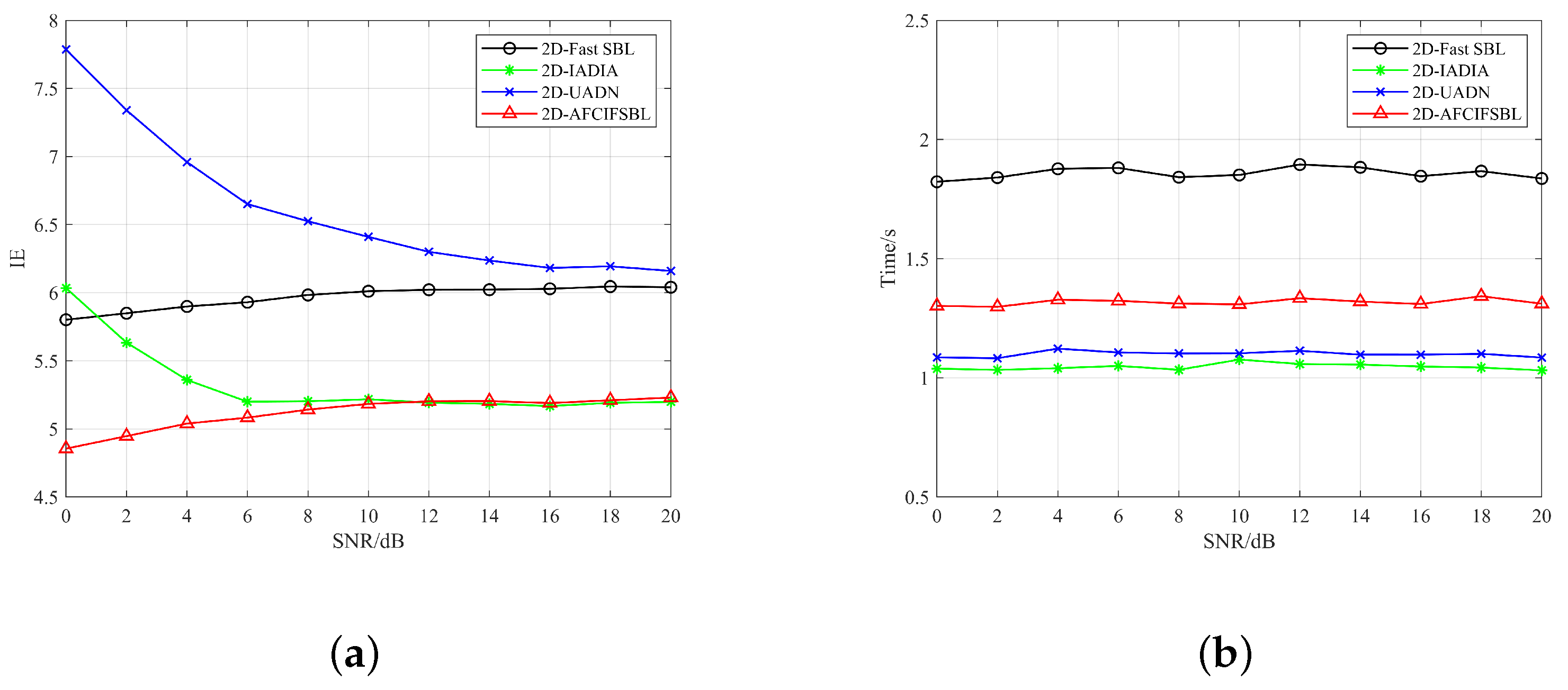
Figure 13 illustrates the quantitative performance comparisons of aforementioned four methods under two evaluation metrics of image entropy and computation time over 100 Monte Carlo trials with the SNR ranging from 0 to 20 dB. The curves in Figure 13a reveal that compared to the 2D-Fast SBL and 2D-UADN methods, the proposed 2D-AFCIFSBL algorithm achieves imaging results with the lowest image entropy, further demonstrating its excellent imaging performance. Additionally, under high SNR conditions, the proposed 2D-AFCIFSBL method exhibits comparable image entropy to the 2D-IADIA method, whereas the 2D-IADIA method has higher image entropy at low SNR levels, suggesting that the 2D-AFCIFSBL method has a certain resistance to noise. In fact, SBL-based methods like 2D-Fast SBL and 2D-AFCIFSBL exhibit consistent performance regardless of SNR variations. In contrast, ADMM-based iterative optimization algorithms, such as 2D-UADN and 2D-IADIA, demonstrate increased image entropy under low SNR conditions. In terms of processing time, as shown in Figure 13b, both the 2D-AFCIFSBL and 2D-Fast SBL methods require more computational time compared to the 2D-IADIA and 2D-UADN methods. This can be attributed to the fact that the 2D-UADN and 2D-IADIA methods are iterative optimization algorithms based on ADMM, which typically exhibit faster computational speeds than sparse Bayesian algorithms like 2D-Fast SBL and 2D-AFCIFSBL. However, compared to the 2D-Fast SBL method, the 2D-AFCIFSBL method has higher computational efficiency in accomplishing the reconstruction task. It demonstrates that the 2D-AFCIFSBL method can improve computational efficiency without compromising imaging performance.
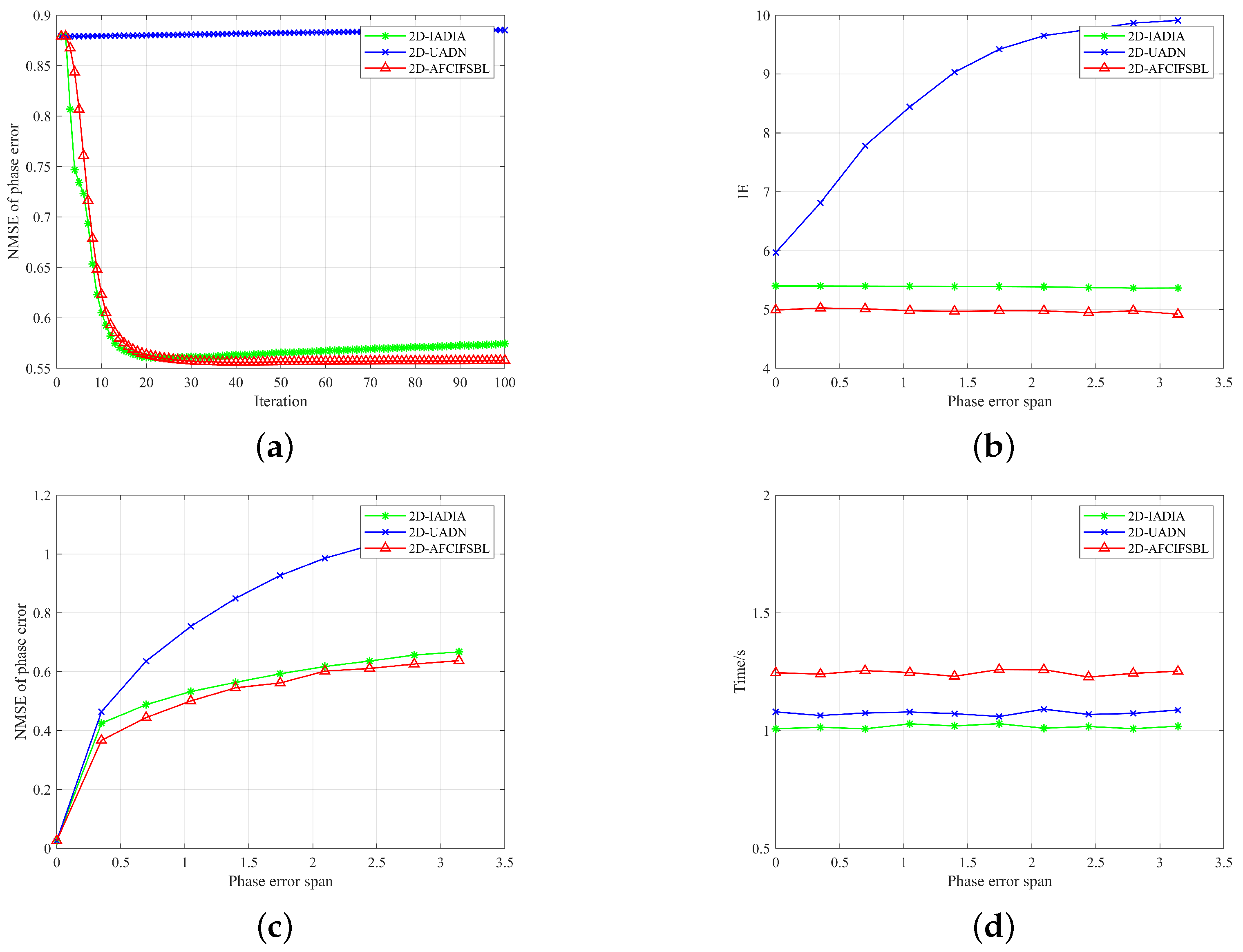
Finally, we analyzed the performance of different algorithms in estimating phase errors, as shown in Figure 14. The range of variance of the phase error is set to 0 π , and the 2D SPR is set to ( 0.8 , 0.8 ) . Figure 14a shows the convergence curve of the estimated phase error with the variance of the phase error set to π / 2 . It can be seen that 2D-UADN has a larger NMSE due to its inability to estimate the phase error between subpulses. Both 2D-IADIA and 2D-AFCIFSBL have the ability to estimate 2D phase errors; therefore, the NMSE is relatively small. Figure 14b shows the impact of the variance of phase error on the entropy of ISAR images. Figure 14c shows the impact of the variance of phase error on the phase error estimation. As the phase error increases, 2D-UADN significantly deteriorates due to its inability to estimate the phase error between subpulses. Figure 14d shows the impact of the variance of phase error on runing time.

4.2. Experimental Results on Measured Dataset

The measured dataset of the Yak-42 aircraft is collected by an X-band radar which transmits LFM signals with a central frequency of 10 GHz and a bandwidth of 400 MHz [30]. The complete radar echoes consist of 256 pulses with each pulse comprising 256 samples. After traditional range alignment and phase compensation, the received echo dimensions are 256 × 256 . However, these echo data are not a stepped frequency signal, so we obtain the equivalent stepped frequency signal by conducting the inverse Fourier transform on the range dimension of the original data. Typically, the linear stepped frequency signal can be considered a specific instance of a random stepped frequency signal. Therefore, we utilize the Yak-42 aircraft measured dataset to validate the imaging performance of the proposed 2D-AFCIFSBL method in this subsection. In this experiment, we only compared the imaging results under the random phase error, where the variance of the amplitude is π / 2 . In addition, we set the SNR of the experiment to 20 dB by adding complex-valued Gaussian noise into measured data.
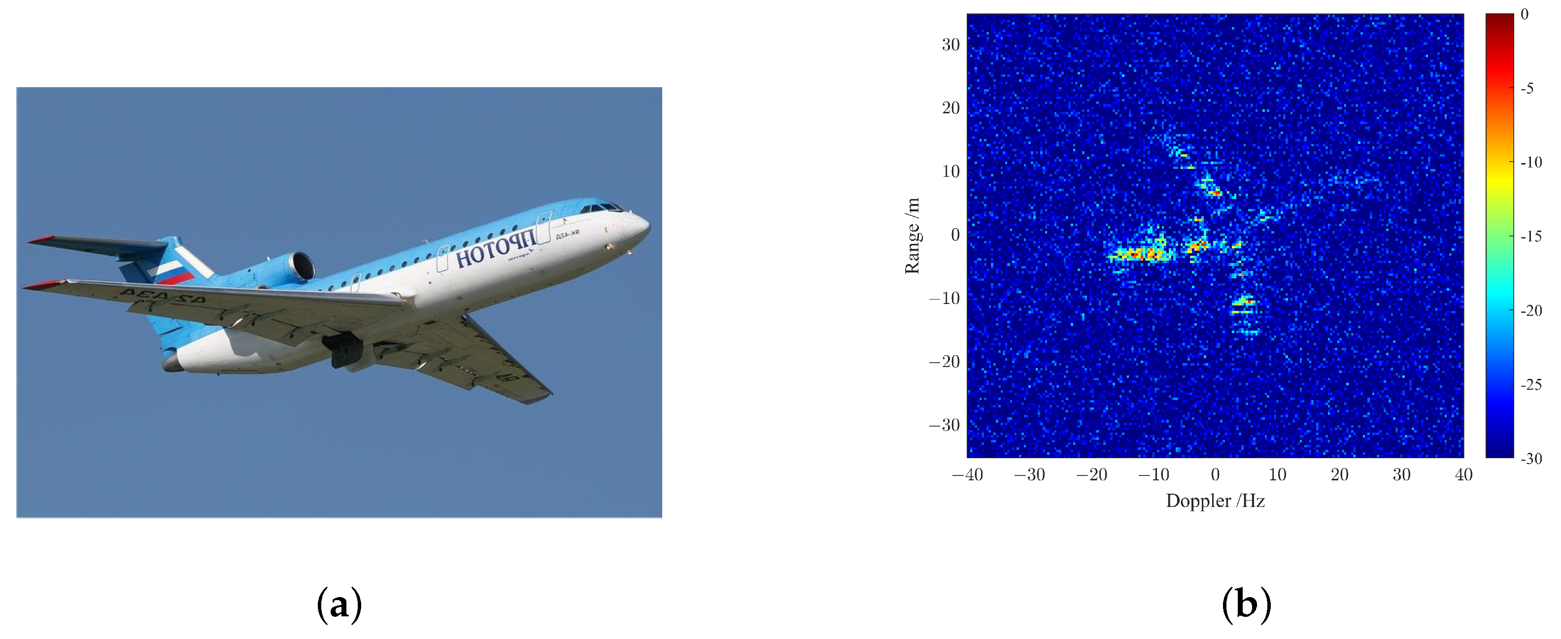
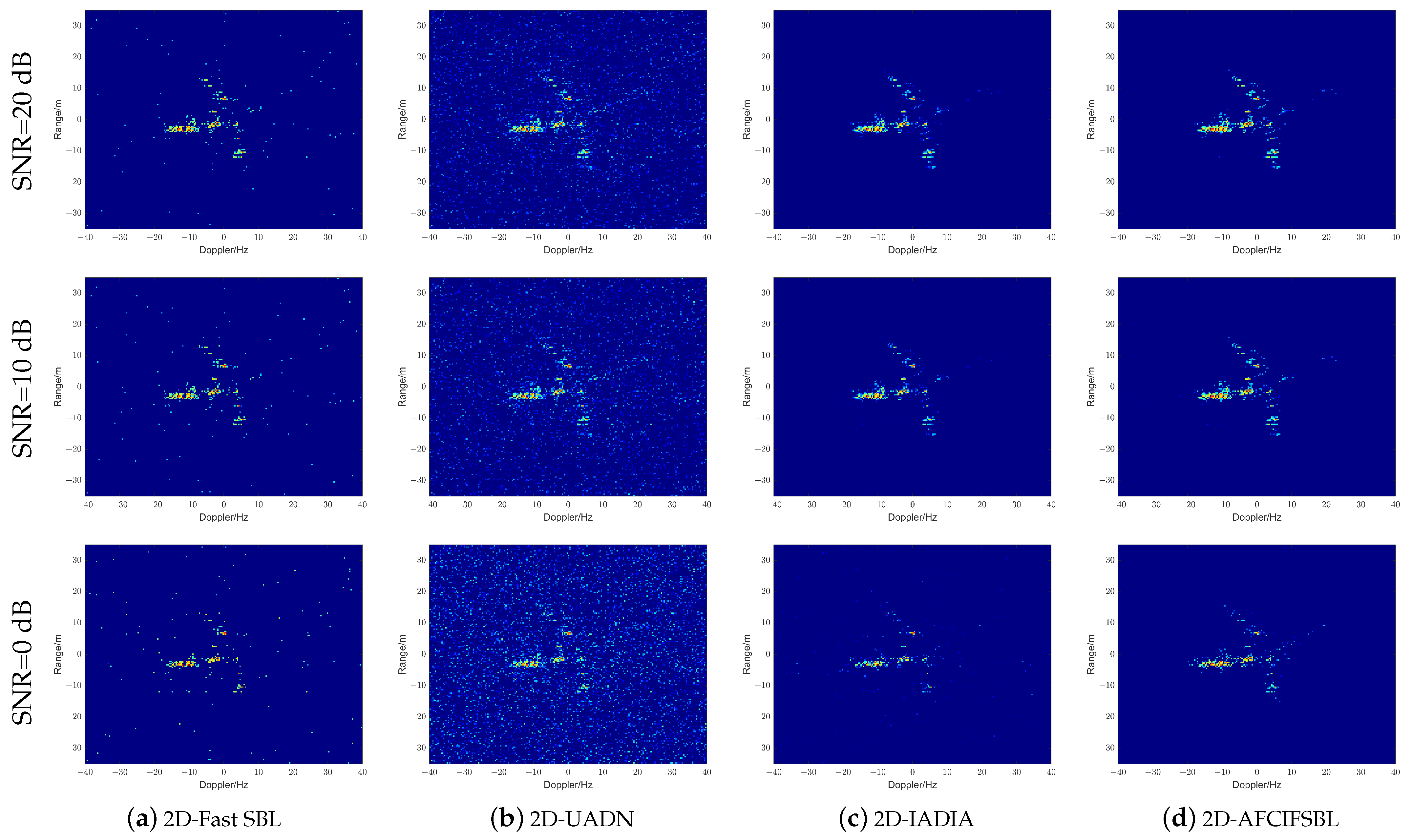
First, the real image of the Yak-42 aircraft and its ISAR imaging result acquired by the 2D range-Doppler method with a complete measured dataset are demonstrated in Figure 15a and Figure 15b, respectively. It is evident from Figure 15b that the phase error that is not fully compensated can lead to severe blurring in the imaging results. In order to acquire sparse data with the SPR of ( 0.8 , 0.8 ) , ( 0.6 , 0.6 ) and ( 0.4 , 0.4 ) , we randomly selected few subpulses and bursts from the complete echo data. And the imaging results acquired by the aforementioned four methods are demonstrated in Figure 16, in which three rows from top to bottom represent the imaging results under the SRP of ( 0.8 , 0.8 ) , ( 0.6 , 0.6 ) and ( 0.4 , 0.4 ) , respectively, and the imaging results of each column are acquired by the corresponding aforementioned methods.
It is evident from Figure 16 that as the SPR decreases, the completeness of the aircraft’s imaging gradually diminishes, and the image of the aircraft’s nose part gradually disappears, which also causes the TBR of the algorithms to gradually decrease, as shown in Table 2. In addition, the 2D-UADN method exhibits the poorest imaging performance with numerous pseudo-scatterers and noise floor across all SPR cases compared to other methods. The 2D-Fast SBL method has slightly better imaging performance than the 2D-UADN method due to its sparse prior resistance to noise. Further, the 2D-IADIA method becomes almost ineffective in case the SPR is ( 0.4 , 0.4 ) due to the appearance of noise floor, while the 2D-AFCIFSBL method continues to produce neat and well-focused images. Table 2 summarizes the experimental results of three evaluation indicators under three types of SPR. Through the analysis of the evaluation indicators in the table, it is evident that the 2D-AFCIFSBL method surpasses the 2D-Fast SBL and 2D-UADN methods in terms of image entropy and TBR by a large margin. The 2D-IADIA method has a similar image entropy to the 2D-AFCIFSBL method, but there is still a gap in TRB. Regarding computational time, the processing time of the four methods on the measured dataset is similar to that on the simulated dataset, as the dimensions of both datasets are the same. Additionally, the imaging speed of the 2D-AFCIFSBL method is observed to be slower than that of the 2D-IADIA method, because the iterative optimization algorithms based on ADMM are faster than the sparse Bayesian learning algorithms. In SBL-based methods, the 2D-AFCIFSBL method is faster than the 2D-Fast SBL method. Nonetheless, the running times of the 2D-AFCIFSBL method remain within the same order of magnitude as the iterative optimization algorithms.
The final experiment was conducted with the SPR of ( 0.7 , 0.7 ) under different SNR conditions, as illustrated in Figure 17, in which three rows from top to bottom represent the imaging results under 20 dB, 10 dB and 0 dB SNR, respectively. It is evident that as the SNR decreases, the imaging results of the 2D-UADN method deteriorate sharply, while the imaging effect of the 2D-Fast SBL method is not as bad as that of the 2D-UADN method due to the sparse prior resistance to noise. For the 2D-IADIA method, as the SNR decreases, many image details are lost, and instead some noise floor begins to appear in the imaging result, which leads to a decrease in the TBR, as shown in Table 3. It can also be observed that even with a decrease in the SNR, the 2D-AFCIFSBL method maintains lower image entropy and a higher TBR compared to other methods. Regarding the running time, each method exhibits similar performance under different SNRs.

5. Conclusions

In this article, we propose a 2D joint imaging and autofocusing method named 2D-AFCIFSBL for SRSF ISAR which can process the 2D echoes directly through matrix operations. First, we model SRSF ISAR imaging using sparse Bayesian learning by imposing a gamma-complex Gaussian hierarchical prior, thereby ensuring the sparsity of the probabilistic imaging model. Then, we increase the speed of Bayesian inference by relaxing the evidence lower bound (ELBO) to avoid matrix inversion, and we further convert the iterative process into a matrix form to improve computational efficiency. After that, phase error estimation is integrated into the ISAR imaging stage, which can be calculated through maximum likelihood estimation. Experimental results on both the simulated and measured datasets have demonstrated that even under low SNR conditions, well-focused images can be achieved by the proposed 2D-AFCIFSBL method in high computational efficiency. In the future, we will concentrate on devising probabilistic models that better align with real-world scenarios, leverage the advantages of deep learning methodologies to find more precise solutions, and explore the potential combination between sparse Bayesian inference and deep learning techniques. Additionally, this paper does not consider the structural information of weak scattering points. We will utilize block sparse Bayesian learning to extract structured information from weak scattering regions in subsequent work.

Author Contributions

Conceptualization, Y.W. and Y.L.; methodology, Y.W. and Y.L.; software, J.S.; validation, J.S.; writing—original draft preparation, Y.W. and Y.L.; writing—review and editing, Y.W. and Y.L.; Supervision, G.Z.; Funding acquisition, G.Z. All authors have read and agreed to the published version of the manuscript.

Funding

This research received no external funding.

Data Availability Statement

The data that support the findings of this research are partly available from the corresponding author upon reasonable request.

Conflicts of Interest

The authors declare no conflicts of interest.

References

  1. Chen, C.-C.; Andrews, H.C. Target-motion-induced radar imaging. IEEE Trans. Aerosp. Electron. Syst. 1980, AES-16, 2–14. [Google Scholar] [CrossRef]
  2. Fennell, M.; Wishner, R.P. Battlefield awareness via synergistic sar and mti exploitation. IEEE Aerosp. Electron. Syst. Mag. 1998, 13, 39–43. [Google Scholar] [CrossRef]
  3. Huang, T.; Liu, Y.; Li, G.; Wang, X. Randomized stepped frequency isar imaging. In Proceedings of the 2012 IEEE Radar Conference, Atlanta, GA, USA, 7–11 May 2012; pp. 0553–0557. [Google Scholar]
  4. Axelsson, S.R. Analysis of random step frequency radar and comparison with experiments. IEEE Trans. Geosci. Remote Sens. 2007, 45, 890–904. [Google Scholar] [CrossRef]
  5. Li, Y.; Lv, G.; Chen, H. The study of multi-false targets deception against stepped-frequency waveform inverse synthetic aperture radar. In Proceedings of the 2008 9th International Conference on Signal Processing, Beijing, China, 26–29 October 2008; pp. 2481–2484. [Google Scholar]
  6. Zhang, L.; Qiao, Z.J.; Xing, M.; Li, Y.; Bao, Z. High-resolution isar imaging with sparse stepped-frequency waveforms. IEEE Trans. Geosci. Remote Sens. 2011, 49, 4630–4651. [Google Scholar] [CrossRef]
  7. Donoho, D.L. Compressed sensing. IEEE Trans. Inf. Theory 2006, 52, 1289–1306. [Google Scholar] [CrossRef]
  8. Tomei, S.; Bacci, A.; Giusti, E.; Martorella, M.; Berizzi, F. Compressive sensing-based inverse synthetic radar imaging imaging from incomplete data. IET Radar Sonar Navig. 2016, 10, 386–397. [Google Scholar] [CrossRef]
  9. Liu, Z.; Wei, X.; Li, X. Decoupled isar imaging using rsfw based on twice compressed sensing. IEEE Trans. Aerosp. Electron. Syst. 2014, 50, 3195–3211. [Google Scholar] [CrossRef]
  10. Zhu, F.; Zhang, Q.; Lei, Q.; Luo, Y. Reconstruction of moving target’s hrrp using sparse frequency-stepped chirp signal. IEEE Sens. J. 2011, 11, 2327–2334. [Google Scholar]
  11. Hashempour, H.R.; Masnadi-Shirazi, M.A.; Arand, B.A. Compressive sensing isar imaging with lfm signal. In Proceedings of the 2017 Iranian Conference on Electrical Engineering (ICEE), Tehran, Iran, 2–4 May 2017; pp. 1869–1873. [Google Scholar]
  12. Hashempour, H.R. Sparsity-driven isar imaging based on two-dimensional admm. IEEE Sens. J. 2020, 20, 13349–13356. [Google Scholar] [CrossRef]
  13. Tipping, M.E. Sparse bayesian learning and the relevance vector machine. J. Mach. Learn. Res. 2001, 1, 211–244. [Google Scholar]
  14. Liu, H.; Jiu, B.; Liu, H.; Bao, Z. Superresolution isar imaging based on sparse bayesian learning. IEEE Trans. Geosci. Remote Sens. 2013, 52, 5005–5013. [Google Scholar]
  15. Duan, H.; Zhang, L.; Fang, J.; Huang, L.; Li, H. Pattern-coupled sparse bayesian learning for inverse synthetic aperture radar imaging. IEEE Signal Process. Lett. 2015, 22, 1995–1999. [Google Scholar] [CrossRef]
  16. Bai, X.; Zhang, Y.; Zhou, F. High-resolution radar imaging in complex environments based on bayesian learning with mixture models. IEEE Trans. Geosci. Remote Sens. 2018, 57, 972–984. [Google Scholar] [CrossRef]
  17. Bai, X.; Zhang, Y.; Liu, S. High-resolution radar imaging of off-grid maneuvering targets based on parametric sparse bayesian learning. IEEE Trans. Geosci. Remote Sens. 2022, 60, 1–11. [Google Scholar] [CrossRef]
  18. Zhang, S.; Liu, Y.; Li, X. Fast sparse aperture isar autofocusing and imaging via admm based sparse bayesian learning. IEEE Trans. Image Process. 2019, 29, 3213–3226. [Google Scholar] [CrossRef]
  19. Yang, J.; Thompson, J.; Huang, X.; Jin, T.; Zhou, Z. Random-frequency sar imaging based on compressed sensing. IEEE Trans. Geosci. Remote Sens. 2012, 51, 983–994. [Google Scholar] [CrossRef]
  20. Wang, H.; Liang, Y.; Xing, M.; Zhang, S. Isar imaging via sparse frequency-stepped chirp signal. Sci. China Inf. Sci. 2012, 55, 877–888. [Google Scholar] [CrossRef]
  21. Ghaffari, A.; Babaie-Zadeh, M.; Jutten, C. Sparse decomposition of two dimensional signals. In Proceedings of the 2009 IEEE International Conference on Acoustics, Speech and Signal Processing, Taipei, Taiwan, 19–24 April 2009; pp. 3157–3160. [Google Scholar]
  22. Li, S.; Zhao, G.; Li, H.; Ren, B.; Hu, W.; Liu, Y.; Yu, W.; Sun, H. Near-field radar imaging via compressive sensing. IEEE Trans. Antennas Propag. 2014, 63, 828–833. [Google Scholar] [CrossRef]
  23. Zhang, Y.; Bai, X.; Li, X. High-resolution isar imaging based on 2-d fast sparse bayesian learning. In Proceedings of the 2021 CIE International Conference on Radar (Radar), Haikou, China, 15–19 December 2021; pp. 43–47. [Google Scholar]
  24. Lazarov, A.; Minchev, C. Isar geometry, signal model, and image processing algorithms. IET Radar Sonar Navig. 2017, 11, 1425–1434. [Google Scholar] [CrossRef]
  25. Zhao, L.; Wang, L.; Bi, G.; Yang, L. An autofocus technique for high-resolution inverse synthetic aperture radar imagery. IEEE Trans. Geosci. Remote Sens. 2014, 52, 6392–6403. [Google Scholar] [CrossRef]
  26. Zhang, C.; Zhang, S.; Liu, Y.; Li, X. Joint structured sparsity and least entropy constrained sparse aperture radar imaging and autofocusing. IEEE Trans. Geosci. Remote Sens. 2020, 58, 6580–6593. [Google Scholar] [CrossRef]
  27. Li, X.; Bai, X.; Zhou, F. High-resolution isar imaging and autofocusing via 2d-admm-net. Remote Sens. 2021, 13, 2326. [Google Scholar] [CrossRef]
  28. Shao, S.; Zhang, L.; Liu, H. High-resolution isar imaging and motion compensation with 2-d joint sparse reconstruction. IEEE Trans. Geosci. Remote Sens. 2020, 58, 6791–6811. [Google Scholar] [CrossRef]
  29. Wang, L.; Huang, T.; Liu, Y. Phase compensation and image autofocusing for randomized stepped frequency isar. IEEE Sens. J. 2019, 19, 3784–3796. [Google Scholar] [CrossRef]
  30. Lv, M.; Chen, W.; Ma, J.; Yang, J.; Ma, X.; Cheng, Q. Joint random stepped frequency isar imaging and autofocusing based on 2d alternating direction method of multipliers. Signal Process. 2022, 201, 108684. [Google Scholar] [CrossRef]
  31. Lv, M.; Chen, W.; Yang, J.; Wang, D.; Wu, X.; Ma, X. Joint 2-d sparse isar imaging and autofocusing by using 2-d-IADIANet. IEEE Sens. J. 2023, 23, 16428–16439. [Google Scholar] [CrossRef]
  32. Zhang, S.; Liu, Y.; Li, X.; Bi, G. Joint sparse aperture isar autofocusing and scaling via modified newton method-based variational bayesian inference. IEEE Trans. Geosci. Remote Sens. 2019, 57, 4857–4869. [Google Scholar] [CrossRef]
  33. Duarte, M.F.; Baraniuk, R.G. Kronecker compressive sensing. IEEE Trans. Image Process. 2011, 21, 494–504. [Google Scholar] [CrossRef]
  34. Tzikas, D.G.; Likas, A.C.; Galatsanos, N.P. The variational approximation for bayesian inference. IEEE Signal Process. Mag. 2008, 25, 131–146. [Google Scholar] [CrossRef]
  35. Duan, H.; Yang, L.; Fang, J.; Li, H. Fast inverse-free sparse bayesian learning via relaxed evidence lower bound maximization. IEEE Signal Process. Lett. 2017, 24, 774–778. [Google Scholar] [CrossRef]
  36. Gao, X.; Liu, Z.; Chen, H.; Li, X. Fourier-sparsity integrated method for complex target isar imagery. Sensors 2015, 15, 2723–2736. [Google Scholar] [CrossRef] [PubMed]
  37. Zhang, L.; Qiao, Z.J.; Xing, M.D.; Sheng, J.L.; Guo, R.; Bao, Z. High-resolution isar imaging by exploiting sparse apertures. IEEE Trans. Antennas Propag. 2011, 60, 997–1008. [Google Scholar] [CrossRef]
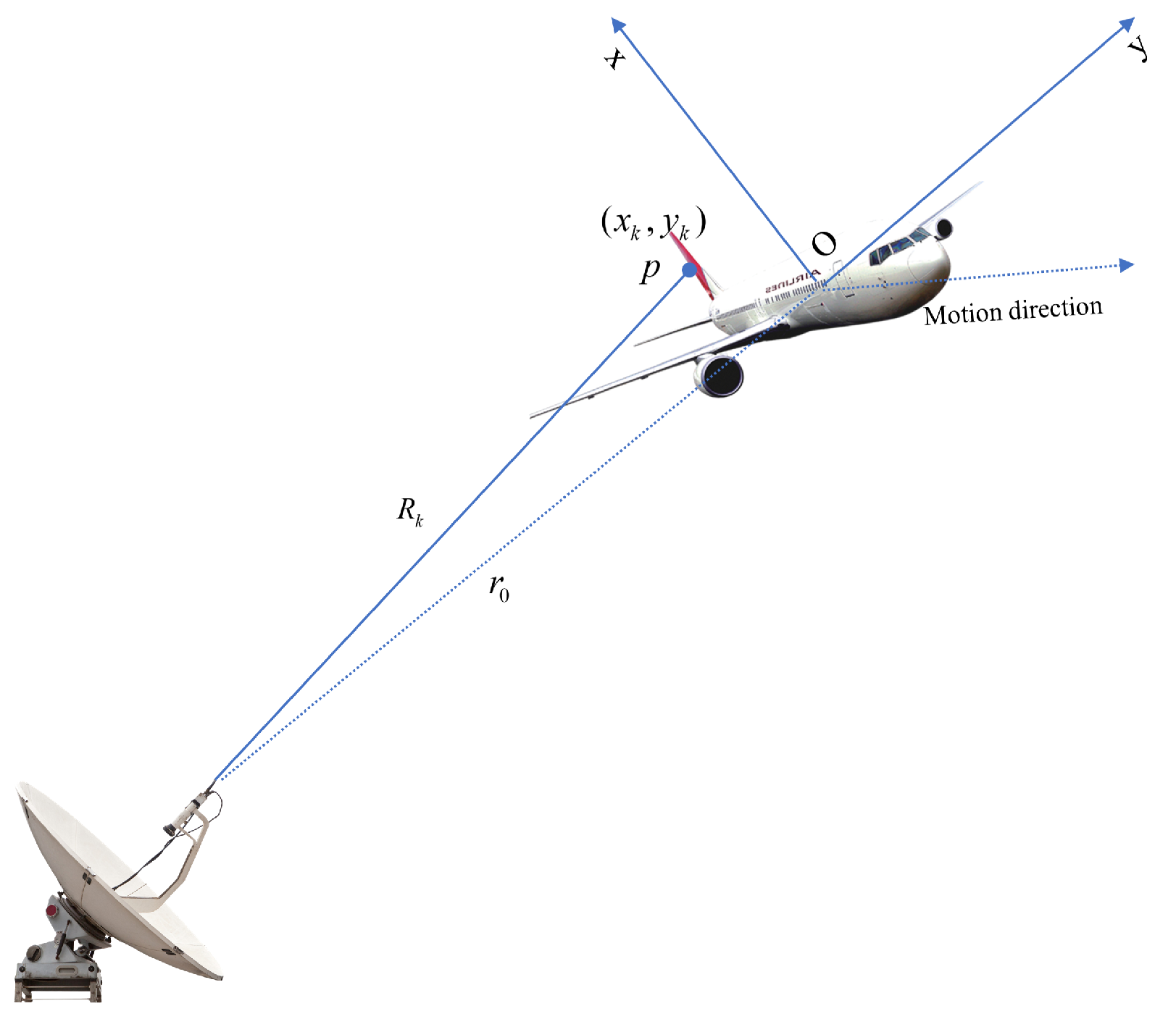
Figure 1. ISAR imaging geometry.
Remotesensing 16 02521 g001
Figure 2. Probabilistic graphical model.
Remotesensing 16 02521 g002
Figure 3. (a) Scattering points of the simulated model. (b) Complete echo data ISAR imaging results.
Remotesensing 16 02521 g003
Figure 4. (a) Random phase error. (b) Linear phase error. (c) Mixed phase error.
Remotesensing 16 02521 g004
Figure 5. ISAR imaging results under ( 0.8 , 0.8 ) SPR with random, linear and mixed phase error.
Remotesensing 16 02521 g005
Figure 6. Image entropy curves added: (a) random phase error, (b) linear phase error, (c) mixed phase error with the SPR of ( 0.8 , 0.8 ) .
Remotesensing 16 02521 g006
Figure 7. ISAR imaging results under ( 0.6 , 0.6 ) SPR with random, linear and mixed phase error.
Remotesensing 16 02521 g007
Figure 8. ISAR imaging results under ( 0.4 , 0.4 ) SPR with random, linear and mixed phase error.
Remotesensing 16 02521 g008
Figure 9. Image entropy curves added: (a) random phase error, (b) linear phase error, (c) mixed phase error with the SPR of ( 0.6 , 0.6 ) .
Remotesensing 16 02521 g009
Figure 10. Image entropy curves added: (a) random phase error, (b) linear phase error, (c) mixed phase error with the SPR of ( 0.4 , 0.4 ) .
Remotesensing 16 02521 g010
Figure 11. ISAR imaging results under 10 dB, 5 dB and 0 dB SNR with ( 0.5 , 0.5 ) SPR.
Remotesensing 16 02521 g011
Figure 12. Image entropy curves under (a) 10 dB, (b) 5 dB, (c) 0 dB SNR.
Remotesensing 16 02521 g012
Figure 13. Quantitative performance comparisons on (a) image entropy, (b) computational time under different SNR.
Remotesensing 16 02521 g013
Figure 14. (a) Convergence curve of the estimated phase error, (b) curve of phase error span vurse IE, (c) curve of phase error span vurse NMSE, (d) curve of phase error span vurse computational time.
Remotesensing 16 02521 g014
Figure 15. (a) The real image of Yak-42 aircraft. (b) ISAR imaging result of Yak-42 aircraft with complete data.
Remotesensing 16 02521 g015
Figure 16. ISAR imaging results under different SPR with 20 dB SNR.
Remotesensing 16 02521 g016
Figure 17. ISAR imaging results under 20 dB, 10 dB and 0 dB SNR with ( 0.7 , 0.7 ) SPR.
Remotesensing 16 02521 g017
Table 1. The main parameters of the X-band RSF radar.
ParametersValue
Initial carrier frequency f c 10 GHz
Synthetic bandwidth B640 MHz
Number of sub-pules N256
Number of bursts N a 256
Stepped frequency Δ f 2.5 MHz
Angular speed ω 0.01 rad/s
Table 2. Numerical evaluation results of measured dataset of Yak-42 aircraft under different SPRs.
SPRMethodsIETRBTime (s)
( 0.8 , 0.8 ) 2D-Fast SBL6.015.551.54
2D-UADN9.14−2.960.93
2D-IADIA5.0522.290.94
2D-AFCIFSBL4.8628.271.17
( 0.6 , 0.6 ) 2D-Fast SBL5.227.851.48
2D-UADN8.62−3.050.91
2D-IADIA4.8120.380.9
2D-AFCIFSBL4.6829.291.1
( 0.4 , 0.4 ) 2D-Fast SBL5.354.861.6
2D-UADN7.93−2.230.94
2D-IADIA4.5517.420.92
2D-AFCIFSBL4.5119.181.07
Table 3. Numerical evaluation results of measured dataset of Yak-42 aircraft under different SNRs.
SNRMethodIETRBTime (s)
20 dB2D-Fast SBL5.1610.321.38
2D-UADN8.70−2.330.93
2D-IADIA5.0219.990.91
2D-AFCIFSBL5.0123.941.08
10 dB2D-Fast SBL5.1110.61.46
2D-UADN8.75−2.720.90
2D-IADIA5.0116.510.98
2D-AFCIFSBL4.9724.471.34
0 dB2D-Fast SBL5.106.141.54
2D-UADN9.21−5.610.92
2D-IADIA4.918.850.94
2D-AFCIFSBL4.6310.381.22
Disclaimer/Publisher’s Note: The statements, opinions and data contained in all publications are solely those of the individual author(s) and contributor(s) and not of MDPI and/or the editor(s). MDPI and/or the editor(s) disclaim responsibility for any injury to people or property resulting from any ideas, methods, instructions or products referred to in the content.