Abstract
The Copernicus Sentinel-6 Michael Freilich (S6-MF) and Jason-3 (J3) Tandem Experiment (S6-JTEX) provided over 12 months of closely collocated altimeter sea state measurements, acquired in “low-resolution” (LR) and synthetic aperture radar “high-resolution” (HR) modes onboard S6-MF. The consistency and uncertainties associated with these measurements of sea state are examined in a region of the eastern North Pacific. Discrepancies in mean significant wave height (Hs, 0.01 m) and root-mean-square deviation (0.06 m) between J3 and S6-MF LR are found to be small compared to differences with buoy data (0.04, 0.29 m). S6-MF HR data are found to be highly correlated with LR data (0.999) but affected by a nonlinear sea state-dependent bias. However, the bias can be explained robustly through regression modelling based on Hs. Subsequent triple collocation analysis (TCA) shows very little difference in measurement error (0.18 ± 0.03 m) for the three altimetry datasets, when analysed with buoy data (0.22 ± 0.02 m) and ERA5 reanalysis (0.27 ± 0.02 m), although statistical precision, limited by total collocations (N = 535), both obscures interpretation and motivates the use of a larger dataset. However, we identify uncertainties in the collocation methodology, with important consequences for methods such as TCA. Firstly, data from some commonly used buoys are found to be statistically questionable, possibly linked to erroneous buoy operation. Secondly, we develop a methodology based on altimetry data to show how statistically outlying data also arise due to sampling over local sea state gradients. This methodology paves the way for accurate collocation closer to the coast, bringing larger collocation sample sizes and greater statistical robustness.
1. Introduction
Sea state observations from satellites are increasing in duration, abundance, variety and applications. The long-term continuous altimetry record is particularly significant in this context, having begun in 1992 and affording us the capability to investigate long-term variability on a global scale from remote observations [1,2]. The continuity and stability of this record is, therefore, of great importance, and to that end, since the TOPEX/Poseidon mission [3] launched in August 1992, the Jason series of satellites [4] has maintained the same reference orbit and ensured a consistency of measurement to the present day. The growing abundance of sea state observations from other missions, spanning a variety of platforms and instruments with heterogeneity in spatiotemporal coverage, further motivates the continuation and maintenance of a consistent long-term record. For example, the European Space Agency (ESA) Sea State Climate Change Initiative (CCI) employs this reference record extensively when intercalibrating missions as part of the production of its multimission sea state Climate Data Records [5].
With the approaching retirement of Jason-3 (J3), ESA’s Sentinel-6 Michael Freilich (S6-MF) mission [6] launched in 2020 and formally succeeded J3 as the long-term altimetry reference mission in April 2022. To ensure smooth operational continuity, S6-MF commissioning involved a unique 12-month S6-MF/J3 Tandem Experiment (S6-JTEX) such that S6-MF followed J3 in the reference orbit, lagging by approximately 30 s, providing the opportunity to generate a substantial record of closely collocated altimetry measurements from these two missions, including sea surface significant wave height (Hs). J3, launched in 2016, obtains measurements of Hs derived from the onboard Poseidon 3B altimeter in low-resolution (LR) mode. Carrying a Poseidon 4B altimeter, S6-MF can similarly acquire measurements of Hs in LR mode. However, the newer instrument is a nadir-pointing dual-frequency synthetic aperture radar (SAR) altimeter designed to provide high-resolution (HR) altimetry measurements. As such, measurements of Hs are made concurrently in both LR and HR modes, providing a valuable opportunity to assess their respective characteristics and, for the first time, to evaluate the performance of the new S6-MF SAR interleaved mode [7] directly against S6-MF LR and J3.
In spite of the advancement in the altimetry measurement record for sea state, questions about uncertainty in observations persist. These stem, in part, from a lack of precise, long-term and quality-controlled direct in situ measurements. While a small number of in situ records date back many decades, their long-term stability remains questionable [8,9], and further, their sparsity limits our knowledge to a small number of global locations, generally far from the coast and in the northern hemisphere. Information about in situ measurement uncertainty is usually entirely absent, and varies between platforms, owing to differences in operating agency, measurement payload, local conditions and so on. While recent efforts have been made to improve quality control information associated with some important records, such as the U.S. National Data Buoy Centre (NDBC) buoy database [10], our enormous reliance on buoy data persists nonetheless, even as the satellite record continues to expand. Dodet et al. [11] conducted an in-depth investigation of uncertainty through intercomparison of measurements with a global set of moored buoys, drawn from the Copernicus Marine Service In-situ TAC (https://www.marineinsitu.eu/dashboard, accessed on 20 April 2024), and model hindcast, using the so-called triple collocation analysis (TCA) [12]. The results from this study established estimates of random error and biases for a range of altimeters, with the lowest errors stated to be around 5%.
Such studies are facilitated by at least two important factors, but these also lead to various limitations in subsequent analyses. Firstly, the analysis of errors is achieved by exploiting in situ measurements at sites in deep water (>50 m). Areas closer to land (<50 km) are excluded to avoid the possibly deleterious effect of radar back-scatter, and the difficulty of analysing over local sea state gradients. Consequently, the analysis of coastal locations, which are often of great interest and unobserved in any other way, are intentionally precluded. Secondly, a large number of collocations improves the statistical robustness of results. Typically many thousands of collocations are required—Dodet et al. worked with some 250,000 collocated data records from numerous missions and spanning three decades. However, although researchers may be able to eliminate the spurious performance of some in situ platforms through their own quality control schemes, ultimately, individual platforms may exhibit quite different biases and errors (see e.g., [11] Figure 3), leading to an analysis that necessarily averages over the entire dataset. The exclusion of platforms is also undesirable since it further reduces sample size and statistical robustness.
The challenge of collocating altimetry observations with buoy (or model) data is characterised by the need to reconcile infrequent snapshots of Hs, derived from rapid along-track sampling, with near-continuous time series of Hs at a quasi-stationary position. At 1 Hz observation frequency, the altimeter covers approximately 7 km of the ocean surface between successive measurements. On the other hand, data buoys tend to derive integral parameters by sampling waves for 10 to 30 min. For practicality, a fixed spatiotemporal match-up criteria for sampling is typically applied to all collocations [13] because the assessment of sites on a case-by-case basis is onerous. Recently, Campos [14] made updated recommendations with respect to spatiotemporal sampling criteria. However, inaccuracies in the match-up, such as representativity error, and site-related problems (e.g., platform mal-operation) can lead to increased uncertainty. In order to better address this, Jiang [15] has proposed a method to explicitly evaluate representativity and environmental and random errors using only altimeter and in situ observations. Using the dataset of the Sea State CCI [16], they conclude that, over a large aggregate global sample for deep-water buoys, different classes of error are approximately equal, and go on to compute altimeter random error more precisely. J3 was found to have similar error characteristics to the previous Jason satellites, with an error increasing with Hs, from 0.15 m (1 m Hs), rising to 0.25 m (7 m Hs). These errors are somewhat smaller than those found by Dodet et al., although, questionably, errors in older altimeters, such as TOPEX/Poseidon, were found to be smaller still.
The aforementioned studies, and others [1,17], limit their analysis to deep-water moorings in order to control for errors that might otherwise be associated with local coastal morphology and resulting gradients in sea state variability. A few studies, however, have attempted to provide analyses of altimeters closer to the coast. Timmermans et al. [18] assessed the limitations of altimetry information to evaluate extremes near the coast. In that case, only a small number of sites were considered, and the collocation methodology did not account for local sea state gradients. Nencioli and Quartly [19] used 17 buoys situated up to a few kilometers from the coast, operated by the National Network of Regional Coastal Monitoring Programmes [20], to validate altimetry observations both from Sentinel-3 SAR and pseudo-LRM modes. They applied a detailed methodology to evaluate how best to compare altimeter and buoy data, concluding that coastal morphology was a hugely important factor in the collocation approach. They investigated sea state gradients in complex coastal regions by computing comparison statistics with buoys from along-track data. Match-up criteria for the final analysis were further informed by the use of a high-resolution coastal hindcast to establish regions of representativity for each buoy. In contrast, using a much larger global set of coastal buoys, Bué et al. [21] computed agreement statistics with a number of altimeters. They employed a methodology that closely collocated altimetry with buoy data based on the distance to coast and concluded that altimeters slightly overestimate Hs in coastal regions.
The use of coastal buoys is desirable in terms of their abundance, compared to their deep-water counterparts, and also creates new opportunities for coastal research. However, collocation has to be meticulous, and disagreements between altimeter and buoy data are often not readily explained by any single factor [19]. In the event of disagreement, no studies cited here explicitly attempt to identify whether buoys themselves may be providing erroneous data. Other aspects of disagreement, such as seasonal conditionality, are also overlooked. Furthermore, high-resolution wave hindcast data that can resolve gradients at similar scales to altimeters, particularly near the coast, are expensive to produce and are unlikely to be available generally. And while altimetry data can be exploited directly to examine sea state gradients [22], to date they have seen little application with respect to understanding and explaining discrepancies and errors with respect to other data sources.
Finally, the aforementioned studies used data from one or more altimeters that did not observe the same sea state concurrently. Data from altimeter–altimeter collocation available in the S6-JTEX tandem phase provides a rare opportunity to compare results from different instruments but under the same conditions. Previously, the Copernicus Sentinel-3A and B satellites were placed in a tandem configuration for six months [23]. Using TCA, Sentinel-3 SAR mode altimetry was found to have to the lowest error by a small margin compared to buoys and ERA5 reanalysis, although the results were limited by few collocations. This experiment also lacked the collocation of both LR and HR data acquisition.
Given the imperative to understand uncertainties in the long-term altimetry record, particularly linked to a transition between reference missions, in this work, we use the collocated S6-MF LR, HR and J3 data from 12 months of the S6-JTEX tandem phase to evaluate uncertainties in observations of Hs. In the locality of the North East Pacific, we undertake a detailed examination of the tandem data, principally via collocation with data from moored buoys located in deep water. After an initial examination of the tandem data in Section 3.1, TCA is presented in Section 3.2. We then proceed to evaluate the effect of the altimeter sampling area on Hs mean bias in Section 3.3. Subsequently, the impact of individual buoys on analyses of Hs mean bias are examined in Section 3.4, and finally a detailed spatial analysis at selected buoy sites is conducted in Section 4. The implications of these results, particularly with respect to their application to coastal regions, are discussed in Section 5.
2. Data and Methods
In this section, we describe the Hs observations obtained from J3 and S6-MF, and other sea state datasets used in the paper, together with the statistical tools and methods used to evaluate the uncertainties across these different datasets.
2.1. Geographic Location and In Situ Wave Observations
The study area is limited to the eastern North Pacific. We primarily exploit data from a number of moored buoys in this area, considered to be offshore (OS) and in deep water (>50 m). The nine buoys, eight (WMO 46001, 46002, 46005, 46006, 46066, 46059, 46078, 46085, yellow diamonds) operated by the NOAA National Data Buoy Center (NDBC, https://www.ndbc.noaa.gov/, accessed on 20 April 2024), together with Coastal Data Information Program (CDIP, [24], https://cdip.ucsd.edu/, accessed on 20 April 2024) station 166 (WMO 46246), close to the Ocean Weather Station PAPA [25] (grey), are shown in Figure 1, and denoted with large diamond-shaped symbols. Numerous buoys located much closer to the coast are also shown for reference, but, with the exception of WMO 46098 and 46244 (CDIP station 168) operated by the NSF Ocean Observatories Initiative (https://oceanobservatories.org/, accessed on 20 April 2024), data from these are not explicitly analysed.
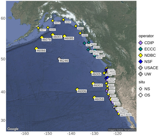
Figure 1.
Study region in the eastern North Pacific. Larger diamonds denote offshore (OS) buoys located in deep water that are used primarily in this study. Numerous buoys nearshore (NS), marked with smaller diamonds, are shown for reference. Colours indicate the agency or organisation responsible for buoy operation.
For buoys operated by NDBC, data are, in fact, available from multiple sources that are known to be inconsistent for some (mostly historic) data. The most comprehensive of these, recently produced by the U.S. Army Corps of Engineers (USACE), is an independent, quality-controlled and consistent (QCC) measurement archive that captures the best available NDBC observations with verified metadata [10]. However, one drawback of its direct use in this study is that data processing of records concluded in August 2021, which lies approximately half way through the S6-JTEX tandem phase. This dictates the use of observations directly from NDBC that may be subject to less rigorous quality checks and that lack metadata. However, substantial impacts upon reliability and stability in these long-term in situ records tend to result from changes that occur infrequently over decadal timescales, such as hull replacement, or significant positional drift. Given the recency and 12-month duration of the tandem phase data examined here, we do not expect data degradation during this time. Furthermore, data from the NDBC-operated moored buoys used in this study were compared with the USACE QCC dataset for the tandem period available, and found to be entirely consistent. The single platform used that is not maintained by NDBC is CDIP 166 (WMO 46246) near Ocean Station PAPA. No additional quality records are available at this site.
To better understand long-term operation and data availability, Figure S1 (Supplementary Material) shows operational coverage of the platforms identified in Figure 1 between 2017 and 2021. OS buoys are shown at the bottom and separated from those closer to the coast by the horizontal black line. Operating agency is denoted by colour, where the overlapping yellow (NDBC) and orange (USACE) bars show the difference in the availability of data passing quality control as a result of the USACE QCC analysis. In addition, the letters A, B and C noted against the USACE data indicate measurement payload changes. These are not considered explicitly in this study but serve to demonstrate the range of variation across platforms. Many other issues, such as changes in hull type and positional drift, can be identified using the USACE data but are not considered here.
2.2. Satellite Altimeter Products: Jason-3, Sentinel-6 LR and HR
Altimeter data from all instruments were obtained during the tandem phase, beginning 18 December 2020 until 31 December 2021. (Additional data during early 2022 were not used.) For J3 only, data from 2017 to 2021 were also employed. The J3 Geophysical Data Record processing baseline F v1.01 [26] provides along-track 1 Hz observations of significant wave height processed from the onboard Poseidon-3B altimeter. In this paper, we use the Ku band-corrected significant wave height swh_ocean, together with quality control indication from swh_ocean_quality, swh_ocean_rms and swh_ocean_numval. For S6-MF, along-track “Non-Time Critical” (NTC) 1 Hz observations of significant wave height for both LR and HR modes are used in the F06 baseline processing from EUMETSAT (https://data.eumetsat.int, accessed on 20 April 2024). The variable ocean_swh is computed from the ocean retracker including all instrumental corrections. Quality control indicators follow the convention of J3, with the same variable names provided. Note that for S6-MF, only a single retracker (“ocean retracker”) is available.
For all altimeter datasets, data quality control is enforced by selecting 1 Hz data points that are flagged as good (swh_ocean_quality = 1), or discarding points with values of swh_ocean_rms above 1 or swh_ocean_numval below 16.
Relationships in Hs variability are established using standard statistical metrics. Temporal separation of observations is limited to 30 min although no adjustments are made, by moving average for example, to better align observations in time in order to avoid smoothing out extremes. The distribution of temporal separation over an increasingly large number of samples tends to a uniform probability distribution.
2.3. Statistical Methods
Standard statistical approaches, including the evaluation of mean bias, linear correlation and linear regression, are employed in order to assess consistency between satellite and in situ data. Note that root-mean-square deviation (RMSD) differs from root-mean-square error (RMSE), which is derived from a linear regression model. In addition, in Section 3.2 and Section 3.4, uncertainty distributions on error variance estimates (from TCA), and Hs mean bias, are estimated using a standard permutation bootstrap method (see e.g., [27]) with 5000 iterations.
2.4. Triple Collocation Analysis
Triple collocation analysis (TCA) [12,28] is a powerful method of evaluating random error where at least three independent measurements of the same quantity are available. Errors associated with each dataset, interpreted as zero mean random error with respect to the ground truth, are calculated without assuming any particular measurement dataset is perfect. However, the validity of its use is dependent on satisfying numerous assumptions, including the independence of the observation errors [12]. Consequently, application to sea state usually employs triplets of data from moored buoys, a numerical model and satellite altimetry, where error independence can be reasonably justified. TCA can therefore be applied to the tandem data; but noting that altimeter–altimeter observation errors are unlikely to be independent, tandem data must therefore be evaluated independently in a TCA. Furthermore, linear dependence between the datasets is also required, which is potentially problematic for the evaluation of S6-MF HR data that are known to exhibit a nonlinear sea state-dependent bias (see Figure 2).
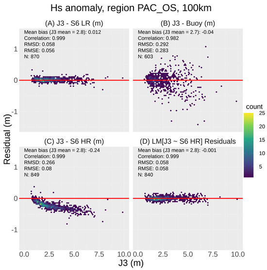
Figure 2.
Significant wave height anomalies between (A) J3 and S6-MF LR, (B) buoy data and (C,D) S6-MF HR for overpasses at OS buoy locations sampled at 100 km radius. The relationship between J3 and S6-MF HR can be modelled robustly with linear regression using simple functions of Hs. Residuals from the fitted model are shown in (D), where outliers have been removed.
The methodology requires that datasets be calibrated to the ground truth, which for wave data is assumed to be obtained from moored buoys. We employ the approach of [28], which differs to that of [12] in regards to data calibration. The latter method may be used to obtain a linear calibration as part of the analysis, whereas, for application in this study, we calibrate the data prior to error evaluation using linear regression. Subsequently, errors are calculated following [28], using Equation (S1) (Supplementary Material). Uncertainty on the error variance estimates is calculated using a bootstrap method applied to the collocation dataset (see, e.g., [27]). Triplets of data are composed of altimeter, buoy and ERA5 reanalysis hourly data [29] on a 0.5-degree grid. ERA5 data are linearly interpolated in space to match the location of the buoy. Note that ERA5 does not assimilate data from either J3 or S6-MF. An example of the geographic collocation setup of a data triplet is shown in Figure S2 (Supplementary Material).
2.5. Analysis of Sea State Gradients at Buoy Locations
In Section 4, sea state gradients at buoy locations are evaluated in the following way. The 9.9-day repeat of the Jason reference orbit results in approximately 36 repeat passes per year, and for J3 up to 180 in total, between 2017 and 2021 (inclusive). Under normal operation, most buoys report a measurement of sea state at least every hour, resulting in possible temporal collocation within 30 min. Where more than one measurement is reported per hour, the measurement closest in time to the altimeter passage is used. No temporal interpolation or smoothing is performed.
At points along J3 tracks that pass within the sampling area of any buoy, the repeated observations can be paired with those from buoys and used to evaluate summary statistics, such as mean bias and correlation. An example of the collocation setup is shown in Figure S2 (Supplementary Material). In order to obtain a spatial gradient, the 1 Hz altimeter data are “binned” along-track with respect to the closet point to the buoy. In this study, a bin size of 10 km is used. Given that the ground separation between successive 1 Hz points is approximately 7 km, up to two 1 Hz points may land in any 10 km bin. For two points, the average is taken.
3. Data Intercomparison and TCA at Offshore Locations
In this section, we intercompare the various Hs observations. In Section 3.1, using standard statistical methods, we evaluate agreement between the measurements of Hs from the tandem datasets and moored buoys. In Section 3.2, TCA is applied to each altimeter dataset, together with moored buoys and ERA5 reanalysis. Finally, in Section 3.3 and Section 3.4, we focus on Hs mean bias between individual buoys and altimeters to identify how the collocation approach affects agreement with each of the buoys in the ensemble. Discrepancies driven by spatial gradients in particular are identified and evaluated through a detailed analysis in Section 4.
3.1. Tandem Data Intercomparison with In Situ Data
The tandem data are collocated along-track, with a 30 s lag for S6-MF. For intercomparisons of wave height over distances of 10–100 km, sea state is not expected to vary appreciably during the lagged period. Given our primary interest of intercomparison with in situ data, initially, comparison of the three tandem datasets is limited to the ground track sections within 100 km of the nine OS buoy sites (see Figure 1). Median values of 1 Hz observations are computed, resulting in a single observation per overpass.
Firstly, LR data from J3 and S6-MF are compared. The anomaly (J3–S6) is shown in Figure 2A, together with a number of statistical measures. A total of 870 overpasses took place, with the data showing near-perfect correlation. A mean bias of ≈0.01 m and an RMSD of ≈0.06 were observed. Outliers are few in number. For Hs greater than 5 m, observations become sparse. In contrast, the comparison between J3 and collocated buoy data (Figure 2B) shows considerable random error and increased mean bias. There also appears to be a negative bias at higher values of Hs. Disagreement is linked to representativity error, local spatial gradients in sea state variability and sampling methodology. These issues are explored in greater detail in Section 4.
A comparison of J3 and S6-MF HR data is shown in Figure 2C. The effect of the sea state-dependent bias in the HR data is evident, resulting in a bias in the mean of −0.24 m. Also, a number of outliers are apparent and likely linked to inconsistent quality control flagging in the S6-MF data. However, linear regression modelling, based on simple functions of collocated J3 Hs, can be fitted robustly and is found to explain 99.8% of the variance. Residuals from such a model are shown in Figure 2D. In this case, residual outliers exceeding 3 s.d. of the distribution are assumed to be spurious and have been removed. Agreement between J3 and S6-MF HR is found to be very similar to S6-MF LR. Mean bias is, in fact, found to be close to zero, with an RMSD of 0.06 m. The linear relationship between the J3 and S6-MF HR is given by,
where the coefficients a, b and c are found to be −0.5654, 1.0930 and 0.4390, respectively.
3.2. Triple Collocation Analysis
TCA can be applied to the tandem data, but while J3 and S6 offer an abundance of data closely collocated in space and time, Figure 2 shows that both LR mode data and HR data are highly correlated (). It is therefore far-fetched to assume that observation errors are independent, which violates an important assumption under the TCA method (see Section 2.4). Each of the three tandem datasets was therefore evaluated independently (together with buoy data and ERA5) in the TCA. In this case, altimeters and ERA5 were pre-calibrated using linear regression with respect to the buoy data, assumed to be unbiased with respect to the ground truth. To remove the nonlinear bias component, S6-MF HR was calibrated in a similar way to Equation (1), but setting buoy data as the response variable in place of J3. Using a 100 km radius, 535 collocations are available. The reduction here with respect to the sample sizes seen in Figure 2 is due to buoy outage. Coefficients of the regression relationships are shown in Table 1.

Table 1.
Calibration coefficients for each dataset, following Equation (1) but where the estimator is with respect to buoy data (). Note, the nonlinear term with coefficient a was included only for S6-MF HR data.
Figure 3 shows the results from TCA using each tandem dataset individually, each together with the OS buoys shown in Figure 1 and ERA5 hourly (0.5 degree) reanalysis. Altimeter estimates of Hs appear to be the lowest, although the sampling error (black error bars show 1 s.d.) is clearly quite large compared to the differences between the datasets, so the results must be interpreted with caution. For example, differences in errors between the different tandem datasets appear to be very small, and are clearly not resolved. To illustrate the impact of data availability, a similar analysis is carried out with the J3 record from 2017 to 2021 (inclusive) and shown in Figure S3 (Supplementary Material). The improvement in statistical robustness from the larger sample size is apparent (3002 vs. 535), and gives rise to some changes in the relative error magnitudes. However, noting the size of the uncertainty estimates on the error variances, even a few thousand samples appears to be insufficient to completely resolve the differences between the tandem datasets in this case. Note that representativity error affects all collocations and may contribute to the higher error values associated with buoy data and ERA5.
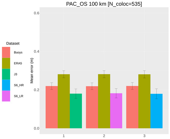
Figure 3.
Standard deviations of estimated mean error variance from TCA for each of the tandem datasets (groups 1, 2 and 3) compared with buoy data and ERA5 reanalysis. Uncertainty in the result is denoted by black bars showing 1 s.d.
To summarise the TCA results, there are a number of issues that affect the implementation and validity of this type of analysis; however, we emphasise two aspects in particular. Firstly, representativity error obscures the true error variance computed with the TCA, and is linked strongly to the collocation methodology. At deep-water sites, where collocation is conducted over, e.g., <100 km, this is generally assumed to be small owing to a high degree of spatial sea state homogeneity in those areas. Secondly, as already noted, large numbers of collocations are required for statistically robust results, particularly where there is little difference between datasets, as is the case here for the tandem data. Seen in Figure 1, even within this particular region, many more buoys are potentially available. However, these are mostly located much closer to the coast, which demands a more detailed collocation methodology. Closer to the coast, gradients in sea state variability are likely to be stronger [19] and consequently have a more dramatic impact on collocation approach.
In fact, we can examine both of these issues in much the same way. We begin, in Section 3.3 and Section 3.4, by evaluating the Hs mean bias between altimeter and buoys to see how individual locations and buoys contribute to the overall bias evaluation. Later, in Section 4, local sea state gradients are evaluated using the altimetry data directly to show how gradients can affect the mean bias under different sampling methodologies.
The results of the TCA and its potential application for the tandem data are discussed further in Section 5.2.
3.3. Hs Mean Bias for Tandem Data
In this section, using all OS buoys, we examine Hs mean bias specifically, and evaluate how this is affected by changes in radius using a typical systematic isotropic sampling method.
The Hs mean bias between S6-MF LR and the buoys is shown in Figure 4. In this case, the sampling radius showing the closest agreement is approximately 60 km (≈−0.008 m), with the bias remaining relatively stable between 35 and 75 km. However, bias with individual buoys can be seen to be highly variable, with only four buoys contributing to the analysis for most sampling radii. The blue shading shows that the altimetry data density diminishes fairly rapidly with decreasing sampling radius. Furthermore, at least two buoys, 46066 and 46059, suffer from data sparsity during the tandem phase (see Figure S1), which gives rise to large biases that are not clearly shown in the figure. These biases are likely associated with stronger seasonal waves.
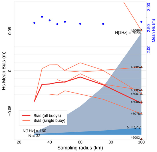
Figure 4.
Overall Hs mean bias (thick red line) for S6-MF LR, and for individual buoys (thin orange lines), as a function of sampling radius. For each buoy, orange triangles show the bias value for 100 km sampling. Total 1 Hz points and total collocations are shown by light blue and dark blue shading, respectively. For reference, blue dots and the coloured scale on the right side indicate the Hs mean. The bias at buoy 46059 lies off the scale (negative), and buoy 46246 has been excluded entirely due to extreme negative bias.
The Hs mean bias for S6-MF HR is shown in Figure 5. The overall behaviour with decreasing sampling radius is remarkably similar although the bias is clearly larger, and on average closer to zero. Statistical noise remains high, owing to the small number of samples, so it is difficult to attribute the difference of 0.01 to 0.02 m between the two S6-MF modes. Finally, for comparison, a similar analysis is shown in Figures S4 and S5 for the one- and five-year J3 records, respectively. For the tandem phase, J3 is extremely similar to S6-MF LR, but showing a slightly increased bias (0.015 m). However, for the five-year record, stability in the mean is much improved and found to lie between 0.01 and 0.02 m.
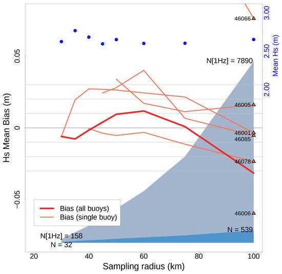
Figure 5.
Similar to Figure 4 but for S6-MF HR. Hs mean bias is slightly larger, and closer to zero on average when compared to S6-MF LR.
To conclude, Hs mean bias appears to be fairly stable even up to 75 km sampling radius. It is clear that bias, calculated using the respective altimeters, shows only small differences ≈0.01 to 0.02 m, which are considerably smaller than the spread of Hs mean bias for individual buoys. In fact, some buoys, such 46246, exhibit very large deviations. We explore the reasons for this in the next section.
3.4. Hs Mean Bias at Each Site
The results in the previous section show, even for deep-water sites offshore, that Hs mean bias varies quite widely depending on which buoy is used. While this is clearly a function of different errors, such as representativeness or possibly environmental effects, bias remains large even as the sampling radius is reduced to recommended scales of around 25 to 50 km [14]. This might be anticipated in coastal areas when sea state gradients can be strong, but offshore, this is somewhat surprising. Fortunately, it is readily possible to use the altimeters to interrogate the buoy data for discrepancy.
Away from land interference, satellite altimeters operate in the same way everywhere, so, compared to a collection of buoys, are not expected to introduce location-specific biases linked to operational variation. This provides a consistent measurement system against which buoy data can be compared. For each of the nine OS buoys, the mean bias with respect to J3 is calculated. To improve statistics beyond the single year of the tandem phase, this analysis exploits the five-year J3 record from 2017 to 2021. Large absolute values of mean bias may indicate the degraded operation of a buoy. In order to assess statistical significance, the sampling distribution of mean bias is obtained using a bootstrap sampling approach. The entire sample from all buoys is used to estimate the population, and data pairs (J3 and buoy) are sampled randomly with replacement. For each buoy, N data pairs are selected, where N is the number of samples observed at that particular location, and a mean bias is calculated. This process is repeated 5000 times, yielding an empirical probability distribution from which the probability of occurrence of the observed mean bias can be estimated. Initially, a sampling radius of 100 km is used, with results shown in Figure 6.
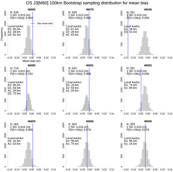
Figure 6.
Each panel shows the observed mean bias (blue line) and how it compares to the estimated probability distribution based on random sampling across all sites. The altimeter tracks, their identifier and their distance of closest approach to the buoy are included in each panel.
The observed mean bias for each buoy is denoted by a blue line. In addition, the number of altimeter tracks, their identifier and their distance of closest approach to the buoy are included in each panel. Note that N samples for each location is approximately the number of collocated tracks, multiplied by 180 (the number of passes in 5 years). The estimated probability of random occurrence of the observed mean bias is also shown.
Given the variety of factors that can contribute to mean bias, results must be carefully interpreted. While the mean bias for most buoys appears small, and consistent with the overall population estimate, the observed mean bias at 46246 is found to be highly improbable. Since, in this case, the minimum buoy–altimeter distances are not large (18 and 51 km), the outlying bias suggests some kind of platform-specific issue. Buoys 46066, 46002 and 46005 all exhibit probabilities around a few percent, also suggesting possible systematic conflict with the altimeter.
However, differences in Hs due to large buoy track separations (up to 89 km in these cases) can contribute to bias, so we expect the results to change with more spatially constrained sampling. The same analysis is therefore conducted for altimeter sampling at 50 km radius, the results of which are shown in Figure 7.
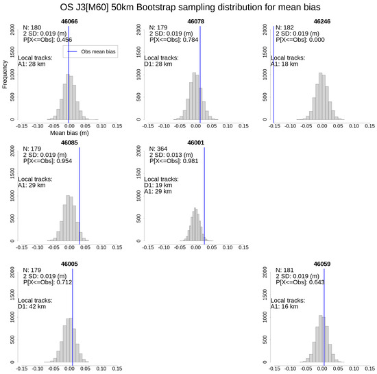
Figure 7.
Similar to Figure 6 but for 50 km sampling. Buoys 46002 and 46006 are excluded due to lack of collocations.
With a smaller sampling radius, fewer observations are made. In fact, 46002 and 46006 are now excluded from the analysis since no J3 tracks lie within 50 km. Furthermore, fewer samples per buoy in general leads to an increase in the variance in the estimated sampling distribution. This reduces our ability to resolve discrepancies. However, with altimetry observations now taken closer to each buoy, we expect to see increased agreement across the collection of buoys, which is in fact the case. The overall mean bias for all buoys is now closer to zero. This can be seen from the sampling distribution shown in each panel, which is shifted by ≈+2 cm. As a result, low bias at some individual buoys, such as 46066 (top left panel), is now entirely consistent with the overall sampling distribution.
However, in spite of the increase in overall uncertainty, a number of buoys still appear problematic. Again, the mean bias at 46246 remains highly improbable. This is consistent with results presented in Section 4.1 that show Hs mean bias is particularly low everywhere, and largely independent of sampling radius. Furthermore, 46001 still appears to be statistically anomalous, in fact it increased from ≈0 to 2 cm. More dramatically, 46085 has swung from a negative mean bias of 4 cm to a positive bias of 3 cm. These changes are perhaps unsurprising because the number of sampled altimeter tracks has been reduced from four to one. Furthermore, a closer look at the site of 46085 reveals a gradient in mean bias, running approximately south to north, that is driven largely by the winter (ONDJFM) conditions. Local spatial gradients are examined in detail in Section 4.
4. Spatial Analysis Using Jason-3
In the open ocean, sea state conditions are generally expected to be homogeneous over a fairly large area around a buoy site. Sampling at 25 km to 50 km has been found to be optimal [14]. Considering the results in the previous section, which show disagreement between altimeters and buoys, for two sites in particular, we apply the approach described in Section 2.5 to examine some comparison statistics. The visualisation using R [30] is provided by ggmap [31]. We first consider the results at the location of 46246, which shows particularly low Hs mean bias, followed by 46085, which showed a bias that changed from negative to positive with decreasing sampling radius. Again, for improved statistical robustness, the five-year J3 record is used.
For reference, the along-track bias and correlation from J3 for all OS buoys (similar to Figure 8) are shown in Figures S6–S14.
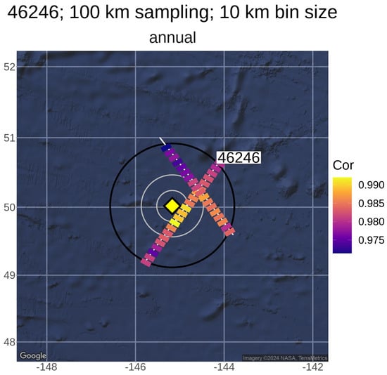
Figure 8.
Using 10 km bins to select 1 Hz observations along-track, linear correlation between J3 and buoy 46246 is shown for the period 2017 to 2021. Reading the figure from left to right, two J3 tracks (white lines), one ascending and one descending, lie within the sampling radius of 100 km (black circle). For reference, grey circles show 50 and 25 km. The highest correlation (>0.99) can be seen on the ascending track closest to the buoy, at approximately 25 km spatial separation.
4.1. Site Analysis at 46246
CDIP 166 (WMO 46246) is a Waverider buoy near Ocean Weather Station “PAPA” [25]. It lies far offshore (49.9N 145.2W) in a water depth exceeding 4000 m. The geographic orientation of the Jason reference ground tracks (white lines, partially obscured) with respect to the buoy location (yellow diamond) is shown in Figure 8. The large black circle shows 100 km radius around the buoy within which altimetry data were sampled. For scale reference, circles with radii of 25 and 50 km are shown in grey colour. Ascending and descending tracks (passing from left to right) provide information in two quasi-orthogonal directions. Satellite observations along both directions are not concurrent, so the joint properties of the sea state along these different paths cannot be determined using these data alone. However, the buoy generally provides a continuous (hourly) time series from which relationships between the two tracks can be inferred independently.
The coloured segments along-track shown in Figure 8 are the correlation between the altimeter measurements and the buoy, calculated in the following way: The position along each track closest to the buoy is used as a reference to define data bins of length 10 km. Following bin allocation, the observations form a set of time series (one series per bin) that can be temporally matched with buoy data to generate standard statistical measures.
Considering Figure 8, altimeter–buoy correlation is shown for all collocations throughout the 2017 to 2021 J3 record (complete “annual” data). The results appear to be physically consistent with good agreement in temporal variation between the two sources. Correlation remains high (>0.98) at most locations along-track with the highest values, approaching unity, at the smallest spatial separation (≈20 km) between altimeter and buoy, on the ascending track. A slight, approximately meridional, gradient is apparent, and statistical noise appears to reduce the smoothness in bin-to-bin variation. Using isotropic sampling, the circles suggest that close to 25 km sampling would capture the highest correlation. However, beyond ≈25 km, the strength of agreement appears to be anisotropic, owing to the spatial gradient.
Figure 9 shows the same analysis approach but for Hs mean bias. In this case, the altimeter measures a lower mean value of Hs than the buoy everywhere (between −0.10 and −0.15 m), even where the altimeter–buoy separation is within 25 km. Unlike correlation, a gradient is not apparent. Following the results found in Section 3.4, which showed this Hs mean bias to be an extreme outlier compared with the complete set of buoys, we conclude that there is some specific deficiency associated with the operation of buoy 46246.
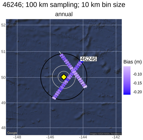
Figure 9.
Similar to Figure 8, but for Hs mean bias.
4.2. Site Analysis at 46085
NDBC buoy 46085 showed an Hs mean bias that changed from negative to positive with decreasing sampling radius. Similar to Figure 9, the along-track mean bias for seasonal (AMJJAS, top panel; ONDJFM, bottom panel) analysis is shown in Figure 10. The gradient observed is strongest during ONDJFM, and suggests that sampling within a radius of 100 km would capture both positive and negative bias. However, as the sampling radius is reduced, the positive bias becomes more dominant, which is the effect also seen in Figure 6 and Figure 7, in Section 3.4.
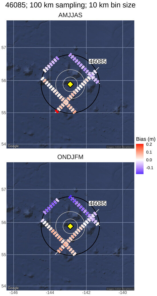
Figure 10.
Similar to Figure 9, seasonal Hs mean bias (AMJJAS, top panel; ONDJFM, bottom panel) between J3 and buoy 46085 is shown for the period 2017 to 2021. A spatial gradient is readily apparent, being strongest in the winter months, where the closest altimeter points are biased positive.
In this case, a spatial sea state gradient is apparent, and clearly affects the choice of collocation methodology. The points along the altimeter tracks closest to the buoy show a positive bias. However, a near-zero bias can be seen at distances in excess of 50 km from the buoy, suggesting that the area of representation for the buoy is anisotropic, with a gradient running approximately south to north. We conclude here that, even offshore in deep water, sea state gradients are relevant to collocation, but that even under recommended criteria (e.g., [14]) disagreement is often present and not easily explained. The analysis here has been limited to Hs mean bias, but we speculate that even greater discrepancy would be found for more extreme sea states.
4.3. Summary
Detailed spatial analysis using altimetry data at buoys 46246 and 46085 has shown that disagreement between altimeters and buoys readily occurs for a range of reasons. In the case of 46246, no explanation is immediately apparent although it appears to be more likely due to buoy maloperation rather than spatial representation. Similar disagreements are readily identified at other buoy sites (see, e.g., Figures S6–S15). For example, the Hs mean bias at 46066 (Figure S6) shows a seasonal variation in bias—positive during AMJJAS and negative during ONDJFM—which is not readily explained.
While a comprehensive description of properties and disagreement at all sites is beyond the scope of this paper, it is clear that a range of error sources are introduced into larger aggregate analyses, like the TCA in Section 3.2, which affects our ability to obtain robust results.
5. Discussion
5.1. Consistency and Uncertainty in S6-JTEX Tandem Data
Accuracy and stability in the long-term altimetry record for sea state are critically important for climate studies. Within this area of study, this analysis demonstrates that differences in the records for both J3 and S6-MF LR are small, and cannot be easily resolved through typical intercomparisons with data from buoys and reanalysis. For example, a mean difference of 0.01 m and an RMSD of 0.06 m between J3 and S6-MF compares with mean differences of 0.05 to 0.10 m, or more, and 0.29 m, respectively, for some widely used buoys. While a sea state-dependent bias affects S6-MF HR data, this issue is linked to instrumental operation and its correction is subject to ongoing technical investigation and revision. However, the correlation between combinations of all three tandem datasets is extremely high, which clearly shows that independent random errors are very small. Uncertainties associated with the collocation methodology, and the buoys themselves, further limit our ability to resolve these differences.
Overall, consistency between J3 and S6-MF appears to be very high and any discrepancies are well within the uncertainty bounds usually associated with intercomparisons of diverse sources of reference sea state data. Although the study area is somewhat limited, any substantial deviation from the results here would be surprising. However, a wider study, involving coastal locations such as those shown in Figure 1, would provide greater statistical robustness and facilitate an examination of whether the results are similar for coastal wave climates.
5.2. Limitations of (Triple) Collocation with Moored Buoys
Studies of sea state variability continue to rely heavily on in situ measurements from moored buoys, although their reliability can often be questioned [8]. The results of this study readily show that well-used data can be statistically questionable. While some programs, such as the Coastal Data Information Program [24] and the National Network of Regional Coastal Monitoring Programmes [20], operate fairly numerous buoys with a focus on reliability and quality assurance for long-term climate records, the primary application is coastal monitoring, usually resulting in buoy placement that is challenging for altimeter collocation. This is unfortunate, since, for short-term studies focusing on a single or joint mission, such as the S6-JTEX configuration, convenient collocations are limited to a fairly small number of deep-water offshore sites. This, in turn, reduces the statistical robustness of results. However, a number of solutions are available.
The results in this paper show how sea state gradients can be examined in coastal areas directly from altimeters, without the need for additional observation or (expensive) coastal numerical modelling. This can be explored further by using concurrent altimeter datasets, which are readily available. This information can be used to develop a reliable coastal collocation methodology, potentially providing access to a large number of coastal buoys, but also has the added benefit of providing valuable information about the coastal oceans. We strongly advocate for advancement in this area. Furthermore, we have also shown how potentially unreliable buoys can be identified, and in this context call for a more explicit interrogation of buoy data on a per-platform basis. This information is also valuable to buoy operators.
Finally, given the challenges of collocation, another avenue to exploit altimetry data, potentially well suited to the tandem phase, where closely collocated altimetry data are abundant, is to try to avoid the issue of collocation with buoys altogether. The recent work of Jiang [15] suggests that double collocation methods (as opposed to TCA) can successfully evaluate uncertainties in altimeters, also providing detailed information about other error sources, including representativity error. Although they suggest that their particular approach will not work well with numerical hindcast data in place of buoys, it may in fact be possible to evaluate absolute errors, similar to those from TCA, by using only two data sources, where one is a calibrated model. In that case, the abundant collocated tandem data could be exploited over the entire ocean, hugely augmenting the available data for analysis.
5.3. Coastal Collocation with Buoys
Few studies address the issue of coastal collocation in detail. Nencioli and Quartly (2019) [19] provide a detailed examination of wave height data from Sentinel-3 (PLRM and SAR HR mode) in the southwestern U.K., following an approach similar to that described in Section 4. However, their methodology benefits from the use of a high-resolution coastal wave hindcast, which is not always available. Furthermore, they consider the in situ buoys to be accurate representations of the ground truth, and do not exploit altimetry data to search for possible conflicts in the way described in Section 3.4. They note, however, that both the distance from altimeter to buoy and the distance from the coast are not typically robust approaches for good collocation. Another recent example [21] attempts a global analysis for coastal collocation by employing a sampling scheme, based loosely on that of [19], whereby buoy data are compared with altimetry at the same distance to the coast. However, while this may be reasonable in some areas, in general, variation in surface wave properties does not follow coastal contours.
A full coastal analysis is beyond the scope of this paper, but to illustrate the point Figure 11 shows that at 46244, lying within 25 km of the coast, the Hs mean bias actually varies seasonally, such that during winter months (ONDJFM) its minimum lies further offshore by approximately 10 to 15 km. We speculate that this is linked to seasonal coastal processes such as wind sheltering or local currents. Regardless of the cause, clearly the gradient is varying seasonally over a distance of some kilometres, so an annual analysis will necessarily average over this gradient, potentially introducing uncertainty. In this case, the method of [21] would seem to be reasonable in AMJJAS when the sea state is similar at both the altimeter and buoy at a similar distance to coast, but would introduce bias during ONDJFM, since the spatial gradient has changed orientation.
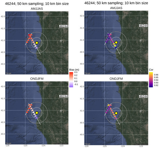
Figure 11.
J3 (2017 to 2021) 1 Hz observations at 46244 binned at 10 km along-track. Mean bias (left panels) and correlation (right panels) are shown. For reference, grey circles show 50 and 25 km radius. Notice that the Hs mean bias lies further offshore by at least 10 to 15 km during winter months.
Furthermore, as shown in Section 3.4, the buoy itself may be statistically questionable. Figure S15 shows another example, buoy 46098, whereby the reference track passes directly over the buoy, and the Hs mean bias can be seen to be positive (≈0.1 m) everywhere, in both AMJJAS and ONDJFM. This is similar to 46246 (Figure 9), but with the added advantage of almost zero representativity error, and suggests a platform-specific bias, again possibly due to degraded operation.
Considering all of these findings, we advocate for the development of a data-informed approach to determine the best collocation strategy, either offshore or closer to the coast. Nencioli and Quartly [19] employ a selection criteria for altimeter–buoy collocations based on threshold values of statistics, such as correlation and RMSE. However, their method is based on comparisons with numerical model hindcast and we suggest that a similar approach could be developed from our analysis, using only altimeters and buoys. Alleviating the need for model data makes the method more regionally accessible. Indeed, sea state gradients determined directly from observations may serve to better validate models. Finally, in this context, it is unclear whether 1 Hz data are most suitable, since clearly within a few kilometres of the coast the altimeter radar footprint will start to be affected. The calculation of gradients using 20 Hz altimeter sampling, following [19], would provide considerably higher spatial resolution.
Supplementary Materials
The following supporting information can be downloaded at: https://www.mdpi.com/article/10.3390/rs16132395/s1.
Author Contributions
Conceptualisation, C.P.G.; methodology, C.P.G. and B.W.T.; formal analysis, B.W.T. and C.P.G.; data curation and production, B.W.T.; writing—original draft prepration, B.W.T. and C.P.G.; writing—review and editing, all authors; funding acquisition, C.P.G. and C.J.D. All authors have read and agreed to the published version of the manuscript.
Funding
The authors thank all the partners of the Sentinel-6 Michael Freilich and Jason-3 tandem Flight Exploitation (S6-JTEX) project, which was funded by the EU and ESA, under ESA Contract No. 4000134346/21/NL/AD. The authors also thank Dr. Jon Blower and the National Oceanography Centre for their support of this research.
Data Availability Statement
Jason-3 data are available from AVISO at https://tds.aviso.altimetry.fr/thredds/catalog.html (accessed on 20 April 2024). Sentinel-6 Michael Freilich data are available from EUMETSAT at https://data.eumetsat.int (accessed on 20 April 2024). Data from National Data Buoy Centre-maintained buoys are available at https://www.ndbc.noaa.gov/ (accessed on 20 April 2024). Access details for the USACE QCC Measurement Archive can be found in [10]. ERA5 data are available at https://climate.copernicus.eu/climate-reanalysis (accessed on 20 April 2024).
Conflicts of Interest
The authors declare no conflicts of interest.
References
- Timmermans, B.; Gommenginger, C.; Dodet, G.; Bidlot, J.R. Global Wave Height Trends and Variability from New Multimission Satellite Altimeter Products, Reanalyses, and Wave Buoys. Geophys. Res. Lett. 2020, 47, e2019GL086880. [Google Scholar] [CrossRef]
- Hochet, A.; Dodet, G.; Ardhuin, F.; Hemer, M.; Young, I.S. State Decadal Variability in the North Atlantic: A review. Climate 2021, 9, 173. [Google Scholar] [CrossRef]
- Fu, L.L.; Christensen, E.J.; Yamarone, C.A., Jr.; Lefebvre, M.; Menard, Y.; Dorrer, M.; Escudier, P. TOPEX/POSEIDON mission overview. J. Geophys. Res. 1994, 99, 24369–24381. [Google Scholar] [CrossRef]
- Scharroo, R.; Bonekamp, H.; Ponsard, C.; Parisot, F.; von Engeln, A.; Tahtadjiev, M.; de Vriendt, K.; Montagner, F. Jason continuity of services: Continuing the Jason altimeter datarecords as Copernicus Sentinel-6. Ocean Sci. 2016, 12, 471–479. [Google Scholar] [CrossRef]
- Dodet, G.; Piolle, J.F.; Quilfen, Y.; Abdalla, S.; Accensi, M.; Ardhuin, F.; Ash, E.; Bidlot, J.R.; Gommenginger, C.; Marechal, G.; et al. The Sea State CCI dataset v1: Towards a Sea State Climate Data Record based on satellite observations. Earth Syst. Sci. Data 2020, 12, 1929–1951. [Google Scholar] [CrossRef]
- Donlon, C.J.; Cullen, R.; Giulicchi, L.; Vuilleumier, P.; Francis, C.R.; Kuschnerus, M.; Simpson, W.; Bouridah, A.; Caleno, M.; Bertoni, R.; et al. The Copernicus Sentinel-6 mission: Enhanced continuity of satellite sealevel measurements from space. Remote Sens. Environ. 2021, 258, 112395. [Google Scholar] [CrossRef]
- Gommenginger, C.; Martin-Puig, C.; Amarouche, L.; Raney, R.K. Review of State of Knowledge for SAR Altimetry over Ocean; Report of the EUMETSAT JASON-CS SAR Mode Error Budget Study. (Reference EUM/RSP/REP/14/749304, Version 2.2, 57pp); Technical Report; EUMETSAT: Darmstadt, Germany, 2013. [Google Scholar]
- Gemmrich, J.; Thomas, B.; Bouchard, R. Observational changes and trends in northeast Pacific wave records. Geophys. Res. Lett. 2011, 38. [Google Scholar] [CrossRef]
- Collins, C.O.I.; Jensen, R.E. Tilt Error in NDBC Ocean Wave Height Records. J. Atmos. Ocean. Technol. 2022, 39, 915–928. [Google Scholar] [CrossRef]
- Hall, C.; Jensen, R.E. USACE Coastal and Hydraulics Laboratory Quality Controlled, Consistent Measurement Archive. Sci. Data 2022, 9, 248. [Google Scholar] [CrossRef]
- Dodet, G.; Abdalla, S.; Alday, M.; Accensi, M.; Bidlot, J.; Ardhuin, F. Error Characterization of Significant Wave Heights in Multidecadal Satellite Altimeter Product, Model Hindcast and In Situ Measurements Using the Triple Collocation Technique. J. Atmos. Ocean. Technol. 2022, 39, 887–901. [Google Scholar] [CrossRef]
- Vogelzang, J.; Stoffelen, A. Triple Collocation; Technical Report NWPSAF-KN-TR-021 Version 1.0; KNMI: De Bilt, The Netherlands, 2012. [Google Scholar]
- Durrant, T.H.; Greenslade, D.J.M.; Simmods, I. Validation of Jason-1 and Envisat Remotely Sensed Wave Heights. J. Atmos. Ocean. Technol. 2009, 26, 123–134. [Google Scholar] [CrossRef]
- Campos, R.M. Analysis of Spatial and Temporal Criteria for Altimeter Collocation of Significant Wave Height and Wind Speed Data in Deep Waters. Remote Sens. 2023, 15, 2203. [Google Scholar] [CrossRef]
- Jiang, H. Random, Environmental, and Representativeness Errors in Ocean Remote Sensing Versus In Situ Data: An Example of Wave Heights From Altimeters. IEEE Trans. Geosci. Remote Sens. 2023, 61, 4205613. [Google Scholar] [CrossRef]
- Piollé, J.F.; Dodet, G.; Quilfen, Y. ESA Sea State Climate Change Initiative: Global Remote Sensing Multi-Mission Along-Track Significant Wave Height, L2P Product, Version 1.1, Centre for Environmental Data Analysis, 2020. [CrossRef]
- Ribal, A.; Young, I.R. 33 years of globally calibrated wave height and wind speed data based on altimeter observations. Sci. Data 2019, 6, 77. [Google Scholar] [CrossRef] [PubMed]
- Timmermans, B.; Shaw, A.G.P.; Gommenginger, C. Reliability of Extreme Significant Wave Height Estimation from Satellite Altimetry and In Situ Measurements in the Coastal Zone. J. Mar. Sci. Eng. 2020, 8, 1039. [Google Scholar] [CrossRef]
- Nencioli, F.; Quartly, G.D. Evaluation of Sentinel-3A Wave Height Observations Near the Coast of Southwest England. Remote Sens. 2019, 11, 2998. [Google Scholar] [CrossRef]
- Mason, T.; Dhoop, T. Quality Assurance & Quality Control of Wave Data. Available online: http://www.channelcoast.org/ccoresources/dataqualitycontrol (accessed on 9 April 2024).
- Bué, I.; Lemos, G.; Semedo, A.; Catalão, J. Assessment of satellite altimetry SWH measurements by in situobservations within 25 km from the coast. Ocean Dyn. 2023, 74, 183–210. [Google Scholar] [CrossRef]
- Passaro, M.; Hemer, M.A.; Quartly, G.D.; Schwatke, C.; Dettmering, D.; Seitz, F. Global coastal attenuation of wind-waves observed with radar altimetry. Nat. Commun. 2021, 12, 3812. [Google Scholar] [CrossRef]
- Clerc, S.; Donlon, C.; Borde, F.; Lamquin, N.; Hunt, S.; Smith, D.; McMillan, M.; Mittaz, J.; Woolliams, E.; Hammond, M.; et al. Benefits and lessons learned from the Sentinel-3 tandem phase. Remote Sens. 2020, 12, 2668. [Google Scholar] [CrossRef]
- Behrens, J.; Thomas, J.; Terrill, E.; Jensen, R. CDIP: Maintaining a Robust and Reliable Ocean Observing Buoy Network. In Proceedings of the 2019 IEEE/OES Twelfth Current, Waves and Turbulence Measurement (CWTM), San Diego, CA, USA, 10–13 March 2019; pp. 1–5. [Google Scholar] [CrossRef]
- Thomson, J.; D’Asaro, E.A.; Cronin, M.F.; Rogers, W.E.; Harcourt, R.R.; Shcherbina, A. Waves and the equilibrium range at Ocean Weather Station P. J. Geopys. Res. 2013, 118, 5951–5962. [Google Scholar] [CrossRef]
- Urien, S.; Bignalet-Cazalet, F. SALP Products Specification—Volume 30: Jason-3 User Products ref. SALP-ST-M-EA-16122-CN Version: 2.1, Centre Nationale d’Etudes Spatiale, 2020.
- Hesterberg, T. Bootstrap. Wiley Interdiscip. Rev. Comput. Stat. 2011, 3, 497–526. [Google Scholar] [CrossRef]
- O’Carroll, A.G.; Eyre, J.R.; Saunders, R. Three-Way Error Analysis between AATSR, AMSR-E, and In Situ Sea Surface Temperature Observations. J. Atmos. Ocean. Technol. 2008, 25, 1197–1207. [Google Scholar] [CrossRef]
- Hersbach, H.; Bell, B.; Berrisford, P.; Hirahara, S.; Horányi, A.; Muñoz-Sabater, J.; Nicolas, J.; Peubey, C.; Radu, R.; Schepers, D.; et al. The ERA5 global reanalysis. Q. J. R. Meteorol. Soc. 2020, 146, 1999–2049. [Google Scholar] [CrossRef]
- R Core Team. R: A Language and Environment for Statistical Computing; R Foundation for Statistical Computing: Vienna, Austria, 2022. [Google Scholar]
- Kahle, D.; Wickham, H. ggmap: Spatial visualization with ggplot2. R J. 2013, 5, 144–161. [Google Scholar] [CrossRef]
Disclaimer/Publisher’s Note: The statements, opinions and data contained in all publications are solely those of the individual author(s) and contributor(s) and not of MDPI and/or the editor(s). MDPI and/or the editor(s) disclaim responsibility for any injury to people or property resulting from any ideas, methods, instructions or products referred to in the content. |
© 2024 by the authors. Licensee MDPI, Basel, Switzerland. This article is an open access article distributed under the terms and conditions of the Creative Commons Attribution (CC BY) license (https://creativecommons.org/licenses/by/4.0/).