Article

Improving Short-Term Prediction of Ocean Fog Using Numerical Weather Forecasts and Geostationary Satellite-Derived Ocean Fog Data Based on AutoML

1
Department of Civil, Urban, Earth, and Environmental Engineering, Ulsan National Institute of Science and Technology, Ulsan 44919, Republic of Korea
2
NARA Space Technology, Seoul 07245, Republic of Korea
3
Graduate School of Carbon Neutrality, Ulsan National Institute of Science and Technology, Ulsan 44919, Republic of Korea
4
Artificial Intelligence Graduate School, Ulsan National Institute of Science and Technology, Ulsan 44919, Republic of Korea
*
Author to whom correspondence should be addressed.
Remote Sens. 2024, 16(13), 2348; https://doi.org/10.3390/rs16132348
Submission received: 19 May 2024 / Revised: 24 June 2024 / Accepted: 25 June 2024 / Published: 27 June 2024
(This article belongs to the Special Issue Artificial Intelligence for Ocean Remote Sensing)

Abstract

:
Ocean fog, a meteorological phenomenon characterized by reduced visibility due to tiny water droplets or ice particles, poses significant safety risks for maritime activities and coastal regions. Accurate prediction of ocean fog is crucial but challenging due to its complex formation mechanisms and variability. This study proposes an advanced ocean fog prediction model for the Yellow Sea region, leveraging satellite-based detection and high-performance data-driven methods. We used Himawari-8 satellite data to obtain a lot of spatiotemporal ocean fog references and employed AutoML to integrate numerical weather prediction (NWP) outputs and sea surface temperature (SST)-related variables. The model demonstrated superior performance compared to traditional NWP-based methods, achieving high performance in both quantitative—probability of detection of 81.6%, false alarm ratio of 24.4%, f1 score of 75%, and proportion correct of 79.8%—and qualitative evaluations for 1 to 6 h lead times. Key contributing variables included relative humidity, accumulated shortwave radiation, and atmospheric pressure, indicating the importance of integrating diverse data sources. The study emphasizes the potential of using satellite-derived data to improve ocean fog prediction, while also addressing the challenges of overfitting and the need for more comprehensive reference data.

1. Introduction

Ocean fog, also known as sea fog or marine fog, is a meteorological phenomenon that causes fog to form over the ocean. Ocean fog consists of tiny water droplets or ice particles formed by the condensation of water vapor [1,2,3]. Due to the Mie scattering process, the presence of these tiny particles causes a substantial reduction in visibility to an extent of 1 km or less. Low visibility raises safety concerns not only for shipping, fishing, and maritime activities but also for traffic controls in coastal regions when ocean fog extends inland [4,5,6]. Such ocean-fog-caused accidents often lead to socio-economic losses, including human fatalities, and thus, it is crucial to predict ocean fog in a timely manner.
To predict fog over the land, including ocean fog intrusion, ground observation time series have been frequently used. Various approaches have been adopted to predict low visibility at ground stations, including ordinary classification [7] and long short-term memory networks [8]. Nevertheless, relying solely on field observations is not a practical method for directly predicting ocean fog, as they are inherently aspatial, resulting in poor expandability to areas without in situ data.
Given the complex interaction between the ocean and atmosphere, people frequently use numerical weather prediction (NWP) to predict the occurrence of ocean fog because it provides visibility predictions for both the land and the ocean. However, the accuracy of NWP visibility forecasts over the ocean is relatively low because the optimization of microphysics and boundary layers for simulating ocean fog varies greatly with time and location [9,10,11]. Several studies have attempted to enhance NWP forecasts in order to accurately simulate ocean fog by coupling multiple models or adopting additional parameters [12,13]. However, the intricate nature of ocean fog phenomena poses a significant challenge to accurately forecasting ocean fog.
Data from satellite scatterometers are consistently assimilated with NWP wind vectors over the ocean, leading to relatively high accuracy in wind forecasts, potentially enabling the use of satellite-detected ocean fog for predicting its movement [14]. Although this method accurately predicted the centroids of ocean fog patches, it failed to simulate the shapes and sizes of ocean fog due to the assumption that the initial shape of the detected ocean fog must remain constant over time.
Other NWP outputs, such as pressure (P), air temperature (Ta), and relative humidity (RH), have systematic errors due to the difficulties of obtaining observational data for data assimilation over the ocean [15,16,17]. These systematic errors limit the effectiveness of NWP models in directly predicting ocean fog. Therefore, to overcome these limitations, the use of data-driven modeling techniques, such as machine learning, could be an attractive solution to predict ocean fog from NWP forecast outputs. Furthermore, using data related to sea surface temperatures (SSTs), such as a simulated SST product or accumulated incoming solar radiation, which is strongly linked to the formation of ocean fog [18,19], can improve the performance of ocean fog prediction when combined with NWP data [12,20,21].
To use such data-driven techniques, it is necessary to have diverse ocean fog reference cases on various spatial and temporal domains. While in situ data are typically obtained at limited locations (generally on the land), satellite-based ocean fog detection may be an attractive approach for collecting a wide range of ocean fog samples in terms of space and time. As ocean fog has distinct optical characteristics, many algorithms for detecting daytime ocean fog were proposed using satellite visible channels as input features [22,23,24,25,26,27]. However, at night, ocean fog also exhibits distinct radiative characteristics in the short and long infrared wavelength channels, leading to the proposal of such channel-based algorithms for nighttime ocean fog detection [28,29]. Daytime and nighttime ocean fog detection models have been combined to produce operational, continuous ocean fog detection. However, inconsistent detection results have often been observed during the transitional period, such as at dawn and dusk, when solar influence changes. To mitigate such an inconsistency, Sim and Im (2023) suggested an algorithm that detects ocean fog continuously, regardless of the time of day, by solely utilizing infrared brightness temperature from geostationary satellite data, resulting in good performance even during transitional periods [6]. As a result, using works of Sim and Im (2023) allows for spatiotemporally diverse and highly reliable ocean fog detection examples [6]. It can also reflect more diverse characteristics of ocean fog than in situ observations, which are limited in both space and time, and help develop generalized algorithms.
Therefore, this study proposed an ocean fog prediction model that considered the spatial and temporal diversity of ocean fog in the Yellow Sea region. Specifically, the aims were to achieve the following: (1) collect ocean fog samples from various locations using satellite-based ocean fog detection; (2) overcome systematic errors in NWP using AutoML, a high-performance data-driven method; and (3) confirm high performance by utilizing SST-related variables with atmospheric variables.

2. Study Area and Data

2.1. Study Area

The study area is the Yellow Sea in Northeast Asia, located between the Korean Peninsula and China. The shallow depth of the Yellow Sea allows the mixing layer to expand downward until it reaches the cold-water layer at the bottom, resulting in abnormal SST drops during warm seasons. This leads to the formation of cold SST zones, even in the summer. The predominant type of fog over the ocean is advection fog, which is primarily formed when warm air passes over a cold surface. Therefore, we selected the Yellow Sea as the study region of focus due to the frequent reports of ocean fog occurrences there [30]. However, the coverage area of the Local Data Assimilation and Prediction System (LDAPS) used in this study is restricted to the Korean peninsula and its surrounding seas. Therefore, the study area was set on the eastern part of the Yellow Sea, extending from 35–40°N to 121.5–127.5°E (Figure 1).

2.2. Himawari-8

Himawari-8 is a geostationary meteorological satellite equipped with a multispectral sensor called the Advanced Himawari Imager (AHI), operated by the Japan Meteorological Agency [31]. This sensor collects data on 16 distinct wavelength channels every 10 min, covering the region of East Asia. The ocean fog detection model developed by Sim and Im (2023) utilizes the infrared channels of Himawari-8 to obtain spatially extensive ocean fog references [6]. Furthermore, when the ocean is unobstructed by clouds or fog, it absorbs solar radiation and accumulates thermal energy. We can estimate the total accumulated solar energy that reaches the ocean by taking into account factors such as the sun’s angle and cloud obstructions. Incoming solar radiation raises SSTs, which might restrict the formation and/or maintenance of ocean fog [32,33,34]. Therefore, we used features that accumulated the hourly level-3 downward shortwave radiation (SWR) product of Himawari-8 from the previous 24 h, 12 h, 9 h to 6 h from the targeting time, the previous day’s total accumulation, and cooling hours as input variables for estimating the short-term heat content of the water mass (Table 1) [18,35].

2.3. Field Reference Data

In order to evaluate predicted ocean fog, ocean fog occurrence data from the cloud aerosol lidar and infrared pathfinder satellite observation (CALIPSO) and the automated surface observing system (ASOS) were used. CALIPSO is a satellite with a sun-synchronous orbit equipped with a cloud-aerosol lidar and an orthogonal polarization sensor. As CALIPSO provides data across the ocean with a wide spatial range, it could be utilized to assess the spatial reliability of predicted ocean fog [36]. CALIPSO uses two distinct laser beams with wavelengths of 532 and 1064 nm to analyze the vertical distribution of atmospheric particle components. The vertical feature mask (VFM) product provides the categorized class profile, which consists of 545 vertical layers. While there is no specific classification for ocean fog, clouds that are located close to the ocean surface or on unusually high ocean surfaces can be considered to be ocean fog. Consequently, the instances of ocean fog were utilized as reference cases after conducting the quality assessment procedure described in Wu et al. (2015) [5].
ASOS is a meteorological and weather measuring system consisting of field-installed measurements on the land. Currently, 103 ASOS stations are operational in South Korea, providing meteorological and weather information on an hourly basis. Among the ASOS data, visibility information of less or equal to 1 km, which has undergone quality checks based on cloud amount and weather information, can be utilized as ocean fog reference data for coastal locations. Baekneoung-do and Heuksan-do stations, respectively located in 38°N to 124.7°E and 34.4°N to 125.3°E, were selected for this study based on their closeness to the coast and the frequency that the ocean fog was reported. Unfortunately, as cloud and weather information are determined through visual inspection by the administrator, it is essential to use the data after careful quality control.

2.4. LDAPS

LDAPS is an NWP model developed by the Korea Meteorological Administrator (KMA) based on the unified model (UM) of the United Kingdom Met Office [37]. LDAPS assimilates surface and upper air observation data via quality assurance processes, resulting in reduced forecasting errors. LDAPS provides data on 70 vertical profiles with a spatial resolution of 1.5 km around the Korean peninsula eight times per day. The forecast data for a time span of up to 36 h, referred to as ‘anal6h’, are produced at 00, 06, 12, and 18 UTC. Similarly, the forecast data for a time span of up to 3 h, designated as ‘anal3h’, along with analysis data, are produced at 03, 09, 15, and 21 UTC. Among LDAPS outputs, surface products highly related to ocean fog occurrence, i.e., air temperature (Ta), relative humidity (RH), pressure (P), u-vector (U), v-vector (V), wind speed (WS), and visibility (VIS), were used as input variables for the ocean fog prediction model [17,38] (Table 1). LDAPS identifies ocean fog when VIS is less than or equal to 1km, called ‘V1KM’, and we used it as a control model.

2.5. HYCOM SST

The hybrid coordinate ocean model (HYCOM) is a comprehensive global ocean reanalysis system that incorporates various data sources, including field observations from instruments like Argo floats, buoys, and ship-based equipment, as well as satellite observations of SST and ocean surface winds. The HYCOM generates outputs of 40 vertical layers that extend to a depth of 5000 m with a horizontal resolution of 1/12° × 1/12°. HYCOM has been extensively studied to assess its reliability in measuring various ocean parameters, including surface salinity and ocean currents [39,40]. The literature has consistently demonstrated that HYCOM performs well in capturing mesoscale ocean phenomena. Regrettably, as HYCOM does not provide a repository of forecast data, the analysis data of the global ocean forecasting system 3.1 version, serving data at 3 h intervals were used under the assumption that the forecast data were closely aligned with the analysis data. Therefore, in this study, the HYCOM SST analysis product was used as an input variable for the ocean fog prediction model after the hourly interpolation of the product (Table 1). We used the temperature difference between SST and LDAPS-derived air temperature (TD) as an input variable in addition to SST, which theoretically indicates the condensation potential of the water vapor [41].

3. Methodology

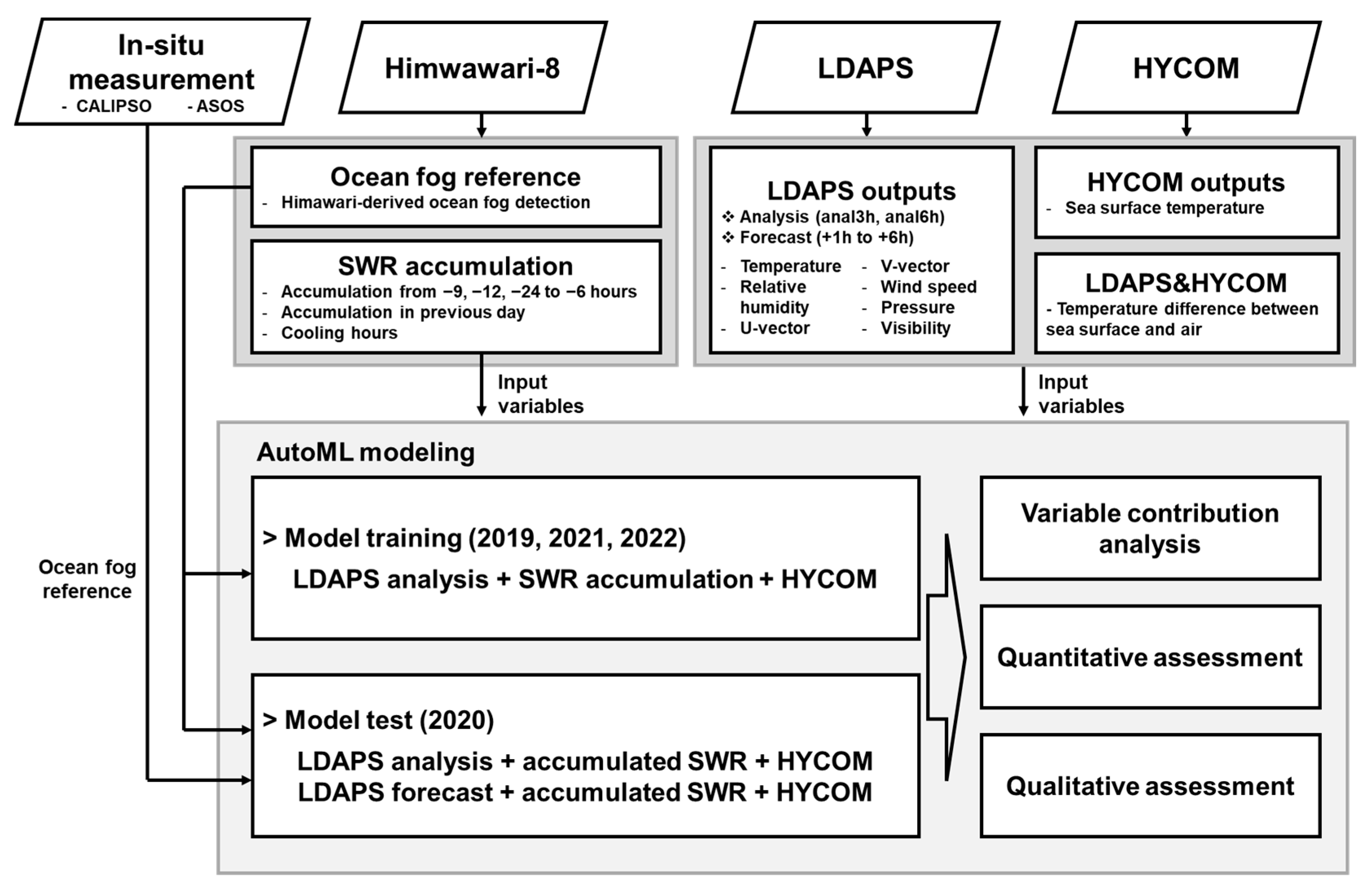
This study proposed an ocean fog prediction model focusing on the Yellow Sea region, which used Himawari-derived ocean fog data [6], LDAPS outputs, and SWR accumulations with machine learning (Figure 2). Because ocean fog mechanisms and behaviors are complex and LDAPS outputs contain systematic errors, an advanced ensemble-based machine learning model known as automatic machine learning (AutoML) was used. Among the 2019–2022 study period, samples from 2020, which had stable and large ocean fog patches suitable for qualitative assessment, were used for testing the model, including quantitative and qualitative assessments, while samples from the other periods were used to train the model. In addition to validation, the variable contributions of input variables to the AutoML model were investigated. CALIPSO and ASOS data, as well as Himawari-derived ocean fog data, were used in the assessment.

3.1. Extraction of Ocean Fog Reference Data

Satellite-based ocean fog detection is highly useful, but its accuracy may be restricted to specific circumstances due to variations in the optical thickness of atmospheric obstructions, leading to potential missed or misclassified ocean fog occurrences [6,23,24]. Therefore, in order to identify ocean fog locations that are consistently stable and reliable, areas where ocean fog has been observed for more than three hours were designated as highly reliable ocean fog areas. Similarly, we designated areas with consistently clear skies for more than three hours as high-reliability clear sky references. We used the ocean fog detection algorithm by Sim and Im (2023), which has been optimized to identify ocean fog in the study area, the Yellow Sea [6] (Table 2). This algorithm demonstrated consistent performance regardless of time and space; thus, it guaranteed stable spatial references by properly filtering out ocean fog and clear skies.

3.2. Modeling

In order to predict the occurrence and persistence of ocean fog in complex and diverse instances with numerical weather data and satellite-based SWR accumulation data, AutoML, a massive modeling technique in the form of an ensemble, was used. Specifically, this study used AutoGluon, an open-source AutoML package developed by Amazon Web Services [42]. AutoGluon uses the sequential stacking of multiple machine learning models with repeating n-fold cross validation to achieve the best performance while mitigating overfitting issues. It also optimizes computational resources through hyperparameter sharing, allowing for highly accurate ocean fog prediction results with limited computing resources [43,44]. It is a model that automatically optimizes for optimal performance and requires no hyperparameters other than the number of sequences, folds to cross-validate, and machine learning tasks to run.
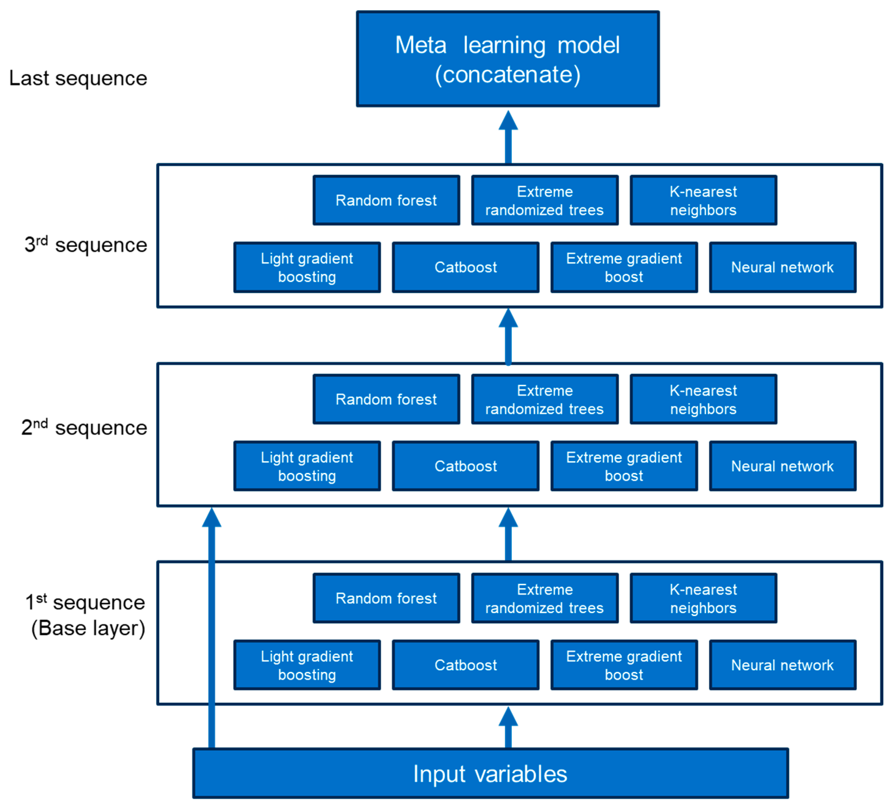
In this study, AutoGluon with four sequences was employed (Figure 3). In the first sequence, known as a base layer, various types of machine learning models (e.g., random forest, extremely randomized trees, k-nearest neighbors, light gradient boosting, catboost, extreme gradient boost, and neural network) were utilized to predict ocean fog using the original input variables. In the second sequence, the same machine learning models used in the first layer were trained to predict ocean fog using the base layer’s results and the original input variables. Following that, the third layer used the same machine learning models as the first layer to predict ocean fog, but only with the second layer’s results. To reduce computing costs, the hyperparameters of each model were shared across these sequences. Finally, in the last sequence, the meta-learning model was trained by concatenating the results from the previous sequence. AutoGluon tuned and fit the hyperparameters and models by repeating the procedure until the user-specified time limit. We used 10-fold cross validation with a time limit of 2 h. The random permutation-based contribution of the input variables used in the modeling was also provided in the form of variable importance, and it was used to estimate how input variables contribute to the model [44,45]. This study utilized samples from LDAPS analysis data for model training and forecast data for model test due to their consistent performance when compared to forecast data. The study period spans from 2019 to 2022; the samples of 2020 were utilized to test the model for both quantitative and qualitative evaluations and the remaining data were used to train the model.

3.3. Evaluation

The model produced binary output, which was either the presence or absence of ocean fog. The model output can be arranged into a 2 × 2 contingency table using the reference data (Table 3). Four accuracy metrics—probability of detection (POD), false alarm ratio (FAR), F1 score (F1), and proportion correct (PC)—were calculated from the table. POD indicates ocean fog prediction performance, which is the proportion of actual ocean fog cases that are correctly classified (Equation (1)), whereas FAR indicates the proportion of cases predicted to be ocean fog that are incorrectly classified (Equation (2)). The F1 reflects how well POD and FAR perform in all aspects (Equation (3)), whereas PC is the proportion of correctly classified cases out of all cases, which represents overall accuracy (Equation (4)). The evaluation was carried out on a case-by-case basis, with each ocean fog and non-fog patch case containing a collection of multiple pixel samples divided into classes based on the majority of the classified area.
P O D = T T T T + T F × 100 %
F A R = F T T T + F T × 100 %
F 1 = 2 × P O D × ( 100 % F A R ) P O D + ( 100 % F A R )
P C = T T + F F T T + F T + T F + F F × 100 %
In addition to the quantitative evaluation, a qualitative evaluation based on the spatial distribution of predicted ocean fog was conducted. The spatial reliability of the prediction was assessed using the CALIPSO data, which provide extensive spatial references for ocean fog. We also evaluated the temporal reliability of the model using the ASOS data, which provide temporally continuous ocean fog references.

4. Results and Discussion

4.1. Quantitative Assessment

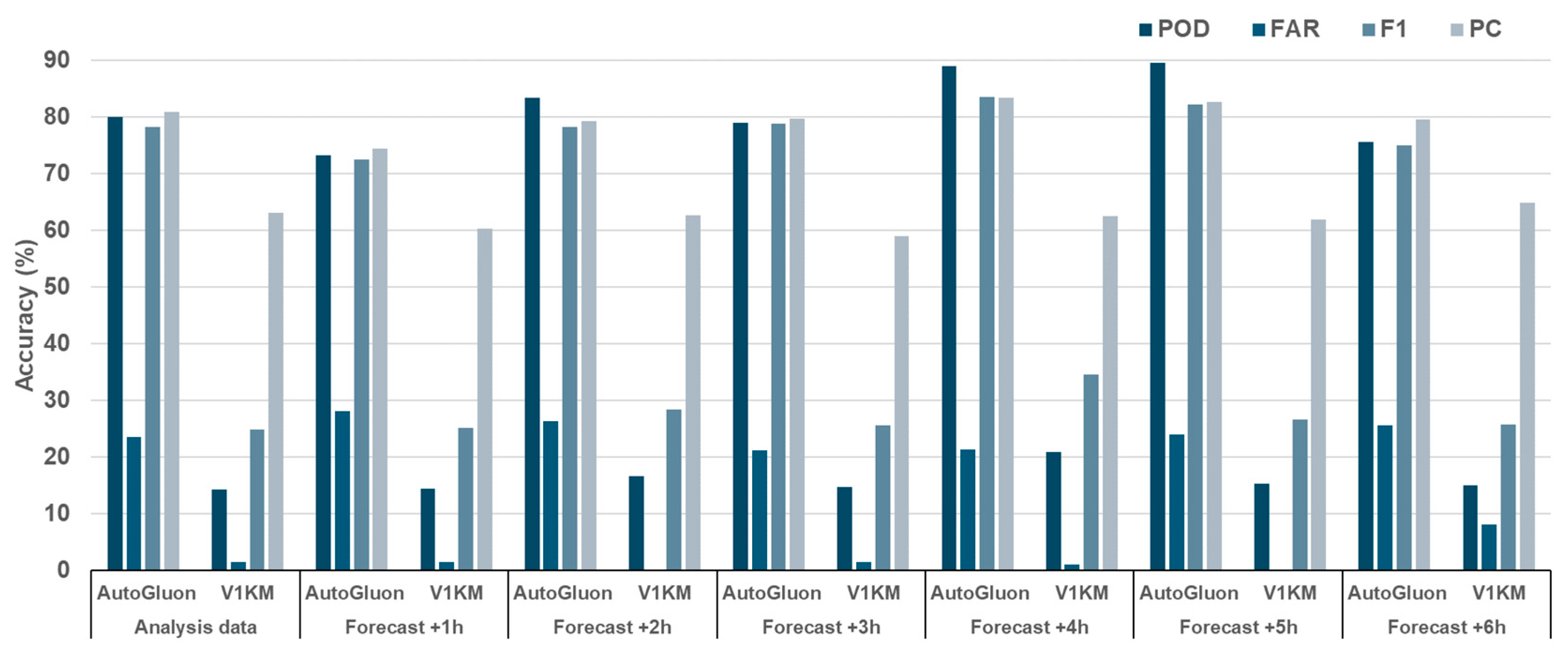
The proposed AutoGluon model performed well, resulting in a POD of 80.0%, FAR of 23.5%, F1 of 78.2%, and PC of 80.9% for the analysis data, whereas V1KM had a POD of 14.3%, FAR of 1.6%, F1 of 24.9%, and PC of 63.1% (Figure 4). AutoGluon outperformed V1KM for most accuracy metrics, but V1KM exhibited outstanding performance for FAR (Figure 4). It was because the V1KM classified the majority of the samples as non-fog, resulting in a lower FAR, as evidenced by the significantly higher PC compared to the lower F1. Prior research utilizing LDAPS data has demonstrated a tendency for overestimating the visibility of LDAPS [37,46,47], suggesting that the V1KM’s accuracy in predicting ocean fog may be compromised due to this factor. Both Autogluon and V1KM exhibited comparable results in terms of prediction accuracy when compared to the analysis data. As the lead time increased to 6 h, performance metrics decreased slightly, but AutoGluon still outperformed V1KM (Figure 4). It is notable that AutoGluon demonstrates superior performance in predicting ocean fog with a lead time of 4 and 5 h (Figure 4). By examining the local time (KST: UTC+9 h, CST: UTC+8 h) of those particular moments, it becomes evident that they correspond to the periods of dawn and dusk. When there is thin ocean fog during that time of day, the detection result may be inconsistent because of solar radiation. However, ocean fog samples that were consistently detected for more than 3 h can be considered to be relatively intense ocean fog cases. The selection of only intense ocean fog cases can be deduced for the purpose of improving the quality of accuracy assessment. While the performance of this study was not validated using the same geographical area and data, the performance metrics from the present study were higher than Kamangir et al. (2021) that had a POD of 65% and FAR of 40% based on deep learning methods with operational NWP results [17] (Figure 4).

4.2. Variable Contribution Analysis

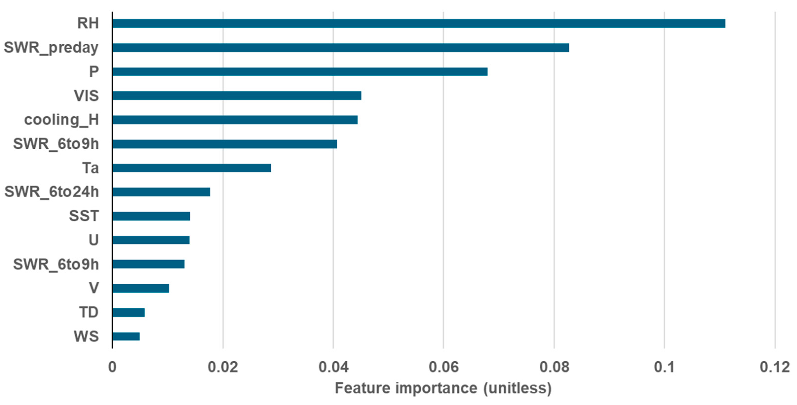
The relative contribution of the input variables was assessed using the random permutation method (Figure 5). RH was the most contributing variable among the 14 input variables, followed by SWR_preday, P, VIS, cooling_H, and SWR_6to9h. RH is used to compute the aerosol extinction coefficient and the dry air aerosol mass-mixing ratio [37]. VIS is determined by the inverse of the total of the extinction coefficients of clear air and aerosol [37]. In other words, RH is more useful than VIS for simulating ocean fog, dominated by condensed droplets, because VIS simulations use other variables [4,48,49]. Even though there was a high correlation with visibility, the value distributions for ocean fog and non-fog samples were similar, with median values of 89.0% and 88.1%, respectively. This suggests that RH, while making a valuable contribution, did not solely determine the prediction of ocean fog, but interacted with other variables.
While SST and TD were anticipated to be essential components in the ocean fog formation mechanism [20], those ranked 9th and 13th because the SWR-related variables (i.e., SWR_preday, cooling_H, and SWR_6to9h) posed more contributing variables (Figure 5). The sun’s shortwave radiation heats the ocean’s surface, but when there are clouds or a sunset, the shortwave warming is blocked and the ocean’s longwave radiation becomes the primary driver, resulting in the cooling of the ocean surface [32,50,51,52]. Simply put, a reduction in SWR accumulation results in greater cooling of ocean water, which promotes the formation and persistence of ocean fog [12,44]. Hence, the notable contribution of SWR_preday in this model suggests that it could be valuable for predicting ocean fog when there is a low amount of overall solar energy accumulated in the preceding day. The variable cooling_H denotes the importance of determining the precise timing of persistent cooling in order to predict ocean fog. Moreover, the variable SWR_6to9h serves as an indicator that the recent utilization of solar energy distribution can be valuable in predicting ocean fog. This is trustworthy because the variable SWR_6to9h varies over time, enabling us to pinpoint the exact location of either ocean fog or non-fog.
Wind is known to significantly influence the development of ocean fog [53,54]. Specifically, gentle breezes are considered crucial for the formation of ocean fog, with advection fog serving as the primary mechanism. However, the evaluation of the ocean fog prediction model revealed minimal influence of U, V, and WS. This can be inferred from the characteristics of the Himawari-derived ocean fog sample used for training; in order to enhance the accuracy of detecting ocean fog, only cases of ocean fog lasting for more than 3 h were chosen, indicating a preference for stable ocean fog instances that have already formed rather than those in the early stages of development. In short, this refers to a situation in which ocean fog samples have been predominantly used at a point where the influence of wind has become insignificant. Furthermore, the P parameter, which serves to indicate a state of macroscopic atmospheric stability, exhibits a high value of model contribution. At lower P, the stability of the atmosphere decreases, leading to an increase in turbulent exchange, a decrease in the stratification of moisture, and a decrease in the presence of liquid water [9,55,56,57]. These conditions are not favorable for the existence of ocean fog. Conversely, high levels of P are advantageous for the formation of both ocean fog and clear skies. It will be incorporated with other factors in ocean fog prediction models.

4.3. Evaluation of Spatial Distribution

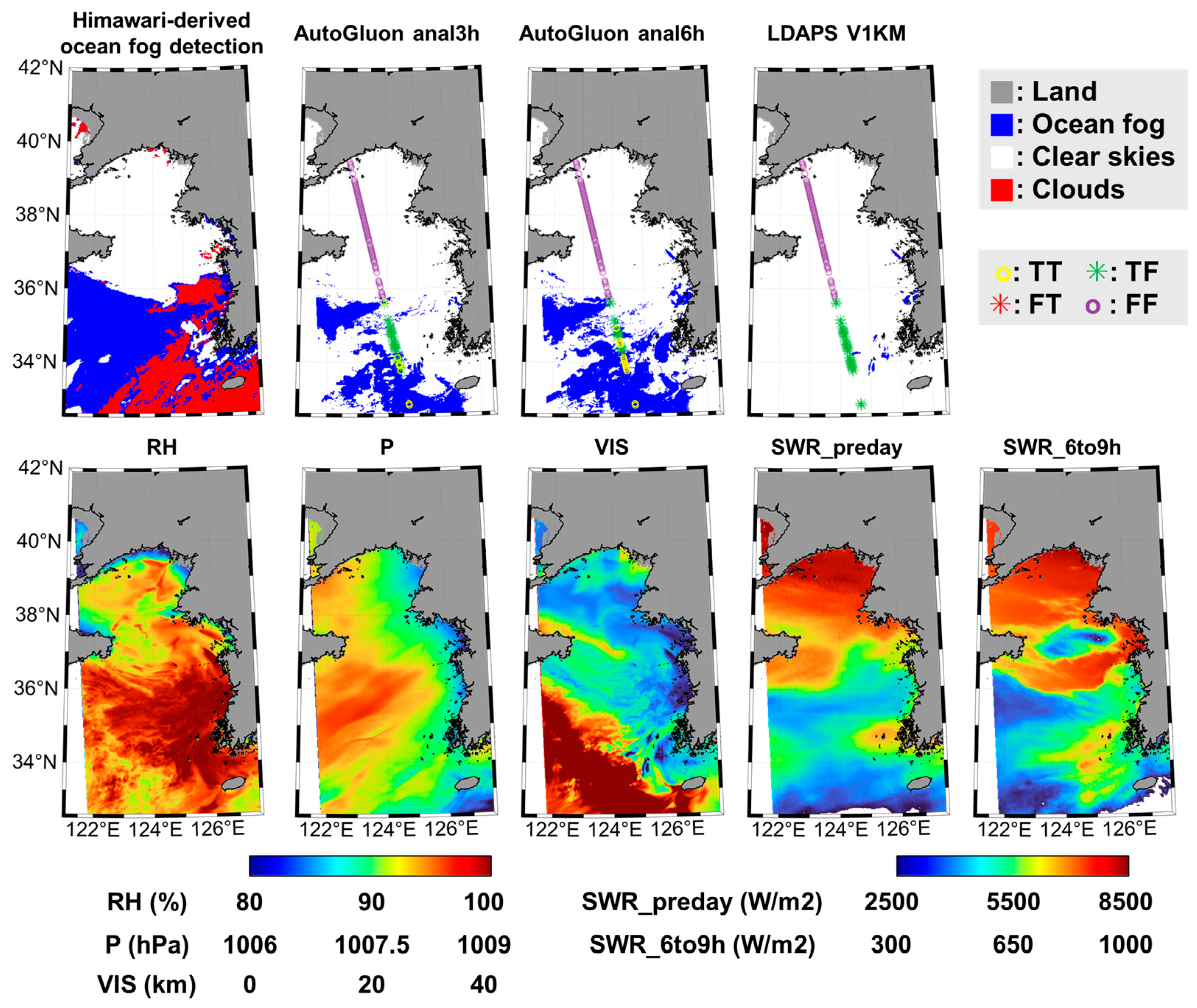
The spatial distribution of the predicted ocean fog was compared to the CALIPSO data in the region characterized by abundant clear skies and ocean fog areas (Figure 6). According to the CALIPSO observation, ocean fog with the unknown class was most prevalent from 34°N to 36°N, clear skies from 36°N to 40°N, and clouds partially with ocean fog from 32°N to 34°N (Figure 7).
We first conducted a comparison between the spatial distribution of the Himawari-derived ocean fog and the predicted ocean fog. According to the results from CALIPSO, the Himawari-derived ocean fog exhibited a mixture of ocean fog and clouds or unknowns below latitudes of 36°N, while the skies were clear in the higher latitudes. All ocean fog prediction models accurately predicted the absence of ocean fog in the clear sky region (Figure 6 and Figure 7). In the ocean fog-dominant region, both AutoGluon using anal3h and anal6h predicted the presence of ocean fog. However, the predicted region was smaller than the detected ocean fog, with the model using anal3h, classifying a smaller area as ocean fog compared to anal6h. Conversely, the results obtained by V1KM indicated a complete lack of prediction for ocean fog in the given region. Despite the presence of clouds, the AutoGluon models predicted the occurrence of ocean fog in the region from 32°N to 34°N. Even though we assume that there is ocean fog beneath clouds, there is no consistent pattern in the distribution of detected and predicted ocean fog. Therefore, we compared the spatial distribution of the input variables that contributed to the prediction of ocean fog in AutoGluon.
The RH values were predominantly low in the non-fog areas and high in the areas where significant ocean fog was detected (Figure 6). When comparing the RH to the ocean fog prediction based on AutoGluon, it was found that some areas with a high RH (~100%) were predicted to have ocean fog. Further, Figure 6 shows a majority of agreement between areas predicted to have non-fog and those with a low RH value (<95%). This indicates that RH plays a crucial role in categorizing non-fog conditions. Regarding variable P, even though it exhibits lower spatial resolution compared to other variables, the distribution of high p values and detected ocean fog locations were found to be similar, as reported in the literature [9,47]. A high level of P, located between 35°N and 36°N and 122°E and 124°E, corresponds to the predicted location of ocean fog (Figure 6). This confirms that P is a valuable factor for identifying the presence of ocean fog on a large scale.
The coastal regions located between 34°N–37°N and 126°E–127°E demonstrate reduced VIS levels that correspond to the detected presence of ocean fog. However, in other regions where ocean fog was detected, there was a consistent tendency to overestimate VIS levels > 20 km. Hence, it is clear that VIS has drastically decreased in the area between 37°N and 40°N, where there were clear skies, compared to the area between 32°N–36°N and 122°E–125°E, where there was ocean fog. After analyzing the patterns of the predicted ocean fog based on AutoGluon and VIS, it was determined that there were no similarities (Figure 6). Therefore, it can be concluded that VIS was not used to predict ocean fog in this particular ocean fog case.
While SWR_preday and SWR_6to9h were not provided for the target time, interestingly, these variables showed notable similarities to the detected ocean fog distribution based on their historical accumulation data. The SWR_6to9h data exhibited low values (<500 W/m2) that closely corresponded to the detected pattern of ocean fog at locations 35°N–36°N and 122°N–124°N (Figure 6). Furthermore, it was discovered that the SWR_6to9h data exhibited similar patterns to the predicted ocean fog area from AutoGluon (Figure 6). AutoGluon identified the region between 32°N–34°N and 122°E–126°E, which has low values of SWR_preday, as an area of ocean fog. However, because the region was classified as cloudy by the ocean fog detection model, a reliable verification could not be performed. Nevertheless, the SWR_6to9h variable in the region of 37°N–38°N, 123°E–126°E exhibits a low value, despite being classified as clear skies by the ocean fog detection model. This suggests that the prediction of ocean fog is not exclusively influenced by the SWR_6to9h variable but rather by a combination of several rules.
Specifically, we compared the CAPLIPSO-based ocean fog case to the ocean fog detection and prediction results (Figure 7). At 32–34°N, where there was a mixture of ocean fog and clouds; the ocean fog detection results were similar to CALIPSO, but the AutoGluon predicted the area as mostly ocean fog. Even though clouds can obscure the presence of ocean fog, the area identified as a mixture of ocean fog and clouds by both CALIPSO and ocean fog detection indicated a high likelihood of ocean fog beneath clouds. In the 34–36°N region, which was a mixture of ocean fog and the unknown class, the ocean fog detection model classified the region mostly as ocean fog, while the AutoGluon model predicted it as a mixture of ocean fog and non-fog (Figure 7). RH and P were favorable for ocean fog in this area, but the SWR accumulation variables, which were the primary influences in this case, did not show strong favorable patterns for this location, leading to the speculation that only a small area was predicted to be ocean fog. V1KM made no predictions for ocean fog in this region. The 36–40°N region, which had clear skies, was identified as non-fog in both ocean fog detection and prediction models (Figure 7). These results confirm that the AutoGluon-based ocean fog prediction model can predict ocean fog over cloudy areas and be sensitive to the distribution of the SWR accumulation variable.

4.4. Evaluation of Spatiotemporal Distribution

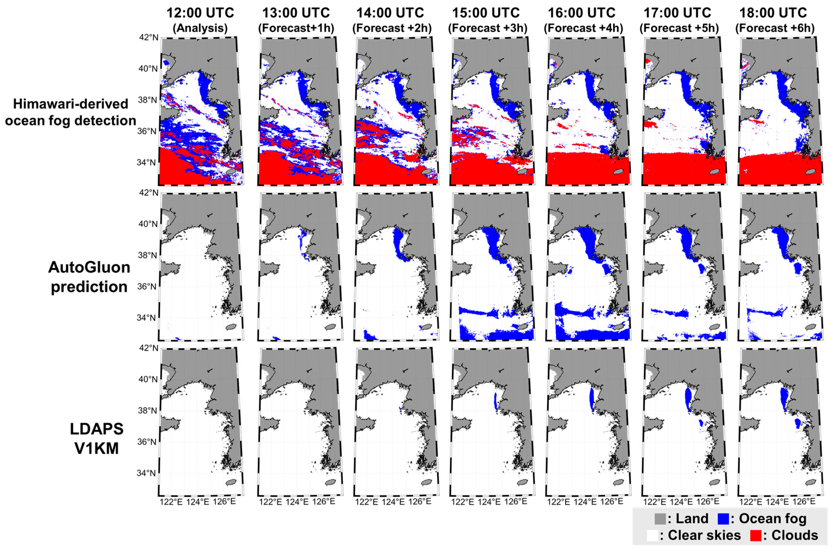
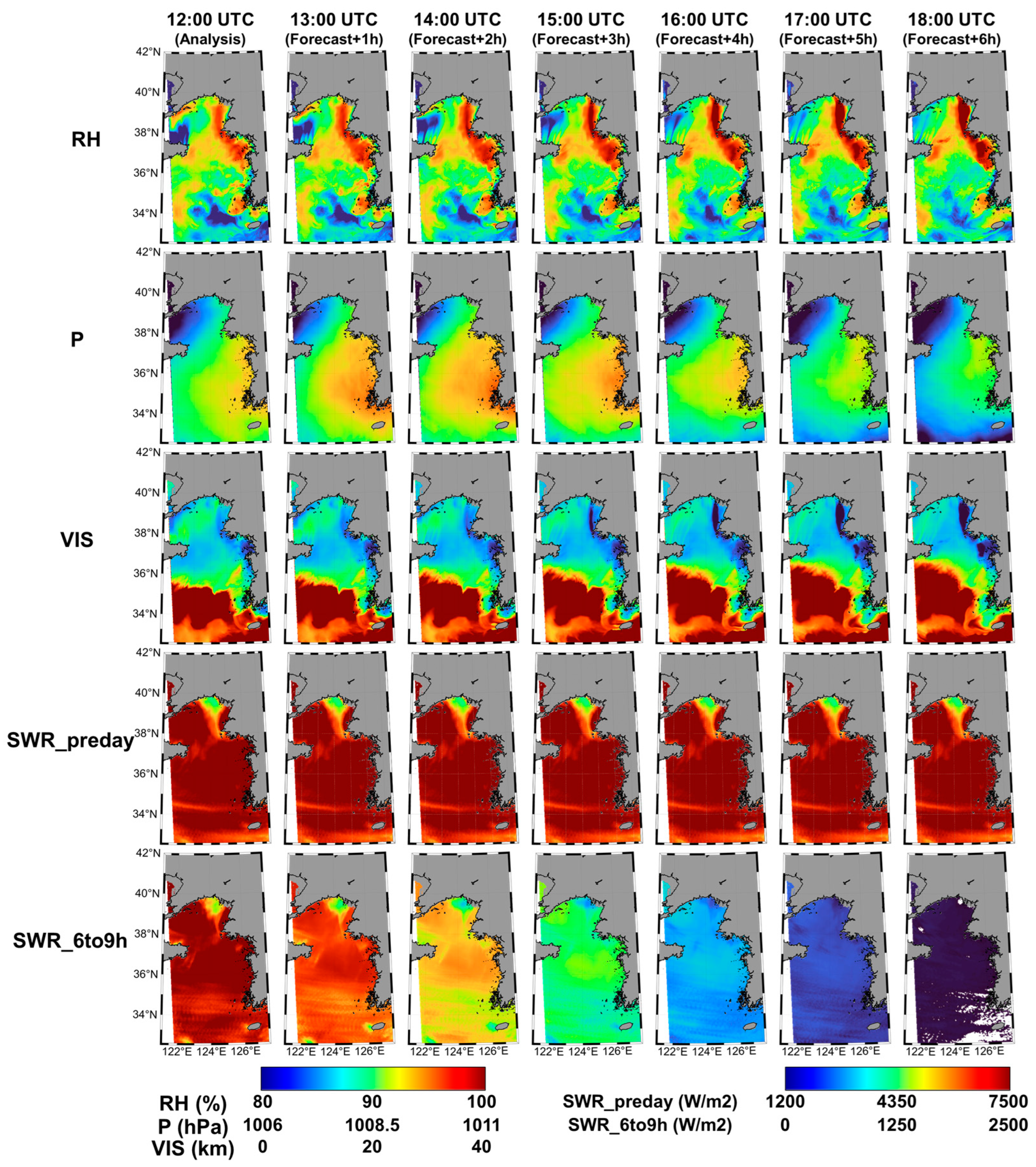
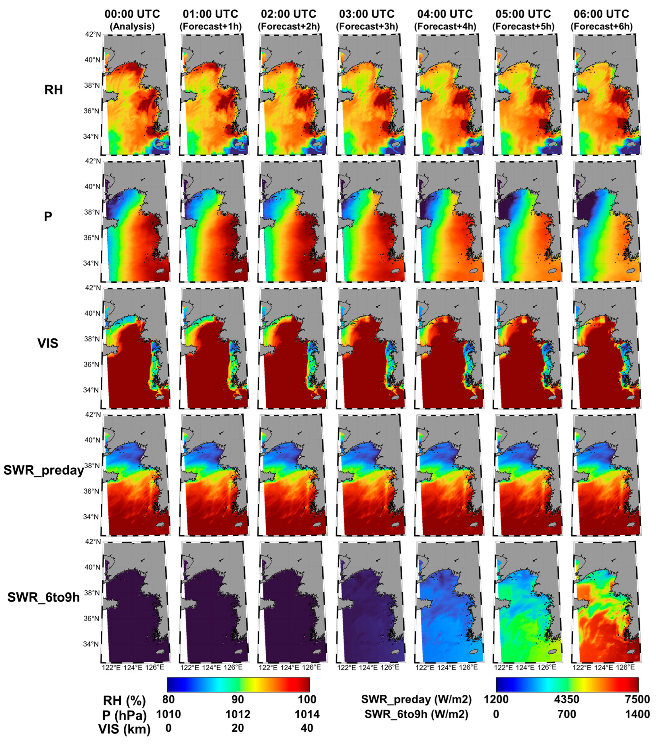
To assess the spatiotemporal continuity and stability of ocean fog prediction models, we chose cases with low cloud cover. First, we investigated the case of ocean fog detected at 37–39°N 124–126°E on 20 June 2020, at 12:00 UTC (Figure 8 and Figure 9). The detected ocean fog was large and persistent, with no cloud contamination, movement, or size variation. However, the ocean fog prediction results demonstrated a different trend, with AutoGluon not classifying any ocean fog at 12:00 UTC, then predicting an ocean fog patch, which grew until the lead time reached 3 h, after which it consistently predicted a similar size patch for the 37–39°N 124–126°E location until the lead time reached 6 h. V1KM did not show noticeable ocean fog areas until the 2 h lead time, and it predicted an ocean fog patch at the 3 h lead time, with the size of the patch increasing until the 6 h lead time. Because AutoGluon as well as V1KM went from undetected to detected and expanded in size for the ocean fog patch, which did not change in size or location, it was assumed that the contribution of LDAPS input variables to AutoGluon’s prediction in this case was significant. To investigate the reasons for the prediction trend of ocean fog patches, we examined the spatial distribution of variables with high contributions in AutoGluon (Figure 9). The time series distribution of the input variables demonstrated that RH and VIS followed a similar pattern for the detected ocean fog patches, as did SWR_preday starting at the lead time of 3 h.
In terms of RH, areas with higher levels seemed to be similar to ocean fog areas determined by Himawari satellite data throughout the observation period. The AutoGluon and Himawari-derived ocean fog distributions exhibited high similarity after the lead time of 3 h, but the earlier time periods showed low similarity, even with extremely high RH values. Specifically, the highest RH value recorded at 12:00 UTC was only at 95%, indicating that the underestimated RH in LDAPS during the analysis and early lead time periods may have contributed an impact in the delayed prediction of ocean fog by AutoGluon. Vis has a similar distribution of low values to RH, but Vis below 1 km becomes noticeable at 3 h lead time, explaining V1KM’s failure to predict ocean fog at 2 h lead time. Furthermore, Vis’s low value area is very small in comparison to the AutoGluon-predicted patches of ocean fog, implying that Vis played no significant role in predicting ocean fog in this case. The SWR_preday, which represents the previous day’s SWR accumulation, is used as the same value by all predictions of AutoGluon on that day. Although low values favor the presence of ocean fog, the spatial distribution differed considerably across all lead times compared to detected ocean fog cases found at 37–39°N 124–126°E. However, there is a line-shaped region at 34.5°N with low SWR_preday values, which AutoGluon predicted as ocean fog with a 2 h lead time. Although it was expected that it would not be used to contribute to the detailed spatial distribution because it is a static variable, it was discovered to have a high contribution at certain moments and is used to predict the detailed spatial distribution of ocean fog based on changes in the contribution degree as the value of other input variables changes.
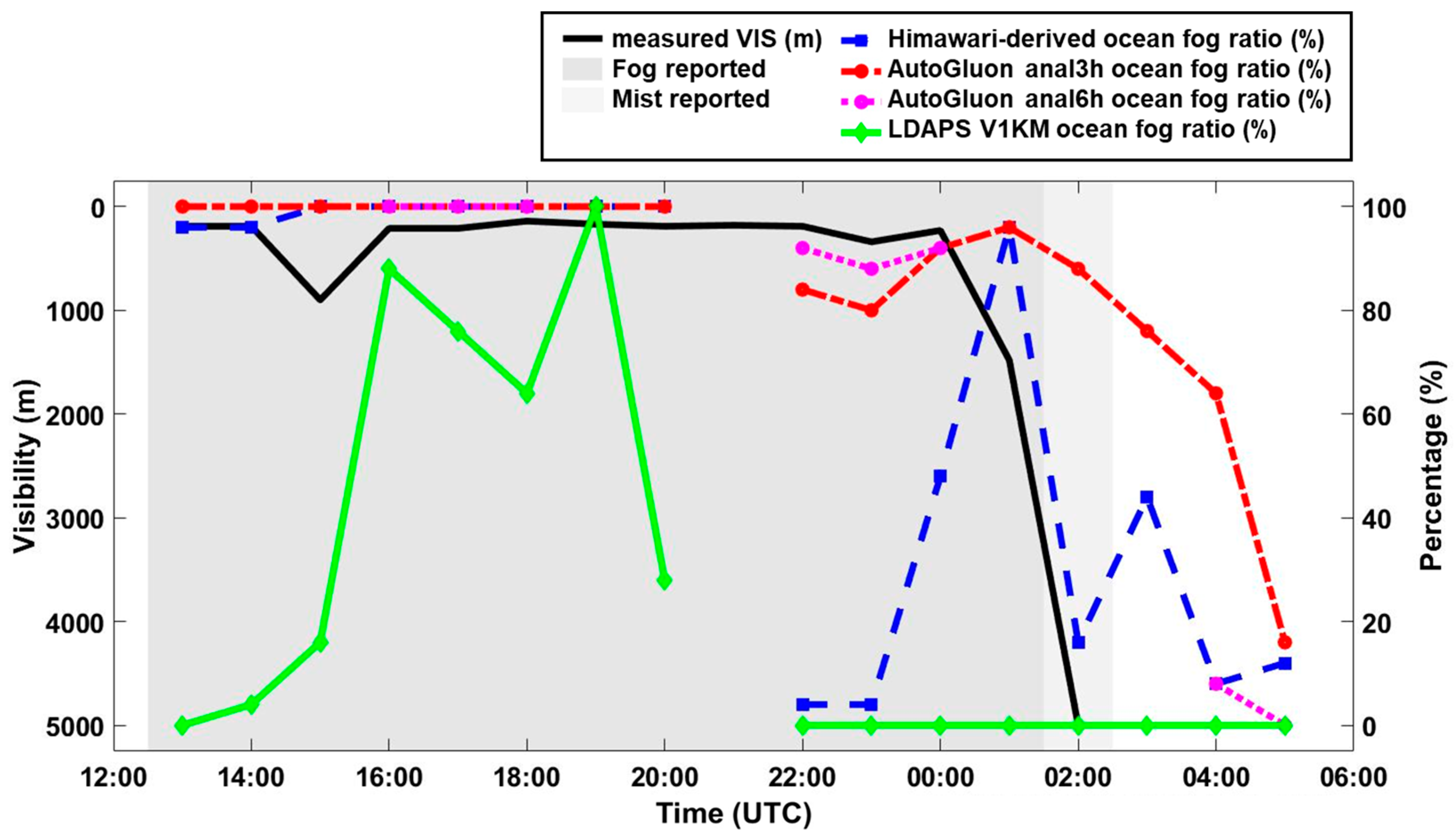
We examined trends in ocean fog detection and predictions at Baekneoung-do ASOS location from 20 June 2020, 13:00 UTC to 21 June 2020, 05:00 UTC, including the period covered in Figure 8 when ocean fog was reported (Figure 1 and Figure 10). Ocean fog was observed continuously from 20 June 2020, 13:00 UTC to 21 June 2020, 00:00 UTC, followed by a 2 h increase in measured VIS, and then non-fog was observed beginning 21 June 2020, 03:00 UTC. More than 80% of the area around Baekneoung-do ASOS was correctly classified as ocean fog until 20 June 2020, 20:00 UTC, but the Himawari-derived ocean fog results were unstable between 20 June 2020, 22:00 UTC and 21 June 2020, 00:00 UTC. This is due to cloud contamination, and as the clouds cleared at 01:00 UTC on 21 June 2020, the percentage of ocean fog detections decreased in favor of non-fog, consistent with the observations. At the time, the AutoGluon prediction model performed well in classifying the majority of the area around Baekneoung-do ASOS as ocean fog until 21 June 2020, 01:00 UTC in both anal3h and anal6h, after which the percentage of space predicted as ocean fog gradually declined. However, the dissipation of ocean fog was delayed by about 3 h compared to the ASOS results, indicating a gap in the different views of ocean fog in the assessment values. This is an unavoidable error when comparing the observed presence of ocean fog in one ASOS region to the percentage of ocean fog in a 100 km2 area. Similar to the results in Figure 8, the predicted area of ocean fog gradually increased from 0% to 100% at 19:00 UTC on 20 June 2020, and then decreased, resulting in a non-fog forecast around the Baekneoung-do station beginning at 22:00 UTC on 20 June 2020. These results show that the AutoGluon-based ocean fog prediction model is stable and performs well regardless of cloud cover.
We investigated the case of ocean fog detected at 34–39°N on 17 August 2020, at 00:00 UTC (Figure 11 and Figure 12). This ocean fog was stationary, unobstructed, yet changing in size. The temporal progression of the Himawari-derived ocean fog indicates a reduction in the overall extent of the foggy conditions between 00:00 UTC and 06:00 UTC, with particular emphasis on the fog along the coastline at 34–37°N and 125–126°E. It is shortly after sunrise in the local time zone (KST: UTC+9h, CST: UTC+8h); therefore, the fog slowly disperses from the eastern direction as the sun ascends [6]. Unlike the decreasing fog that was observed, the AutoGluon prediction indicates a sudden and significant decrease in fog area between 02:00 UTC and 03:00 UTC. Additionally, the V1KM prediction fails to predict any ocean fog at all. In order to determine the cause of the discontinuity and lack of predicted ocean fog, the spatial distribution of the variables that have a significant impact on AutoGluon was examined. Following 03:00 UTC, when the ocean fog patch predicted by AutoGluon has a consistently organized appearance, ocean fog areas resemble the distribution of regions with high values of RH. In addition, the predicted fog’s areas at that time overlaps with the high P regions, demonstrating adherence to the theoretical basis, and low values of SWR_6to9h. The low VIS values correspond to the predicted ocean fog locations, but the area is relatively small and concentrated along the coast. Furthermore, VIS consistently predicts visibility over 40 km regardless of the time of day, implying that VIS overestimates offshore areas and, thus, V1KM may not be a good predictor of ocean fog offshore.
In a whole periodic view, since this period is shortly after sunrise, the time series distribution of SWR_6to9h, where the accumulated SWR value is 0 until 02:00 UTC, exhibits a comparable pattern to the time series discontinuity observed in the AutoGluon prediction. It appears that the AutoGluon model excessively depends on the SWR_6to9h variable, leading to a discontinuity in the time series. This outcome alone might give the perception that the model is overfitting at a specific time. However, areas with persistent ocean fog or clouds lasting more than 3 h also have lower values (~0) for SWR_6to9h. This is reasonable because the cooling effect of longwave radiation creates an optimal condition for the formation of ocean fog [43,50,51]. Nevertheless, the issue of time series discontinuity can pose a challenge; it can be mitigated by increasing the number of training cases in subsequent iterations.
As the presence of ocean fog was also recorded at the ASOS station situated on the Heuksan-do, the time period from 16 August 2020, 19:00 UTC to 17 August 2020, 12:00 UTC was examined (Figure 1 and Figure 13). This period included the dissipation and formation of ocean fog. At the Heuksan-do ASOS station, the ocean fog lasted until 16 August 2020, 22:00 UTC, when it transitioned from ocean fog to mist to non-fog with a significant increase in visibility (Figure 13). Subsequently, the weather conditions remained unchanged, and there was a significant decrease in measured VIS starting on 17 August at 09:00 UTC (Figure 13).
The AutoGluon ocean fog predictions indicate that the dissipation occurs after 03:00 UTC on 17 August from both the anal3h and anal6h data, which is likely caused by the overfitting of the SWR_6to9h variable on the map (Figure 13). Subsequently, the ocean fog was rediscovered at 11:00 UTC, and prediction for the ocean fog aligned with the ASOS observations and persisted until 12:00 UTC. At that moment, the lead time for predicting the occurrence of ocean fog was 5 to 6 h, indicating that the AutoGluon model is effective in accurately predicting ocean fog conditions within a 6 h timeframe.

5. Conclusions

Although predicting ocean fog is important, it remains a challenging subject for numerical simulation due to the complexity of the favorable environment. Consequently, data-driven approaches have been utilized for predicting ocean fog, but they have shown limited performance and generality due to a lack of field data that reflected spatial and temporal variability. In this study, we constructed ocean fog cases based on reliable ocean fog detection results reflecting spatial and temporal variability for the Yellow Sea region and used automated machine learning to predict ocean fog with a lead time of up to 6 h. Based on quantitative and qualitative evaluations, the proposed approach outperformed the operational numerical forecasting model’s visibility-based ocean fog prediction results. Even though it only occurred in a few cases, the proposed model accurately predicted ocean fog under cloud cover. This demonstrated its future potential for removing cloud contamination from ocean fog detection results. According to the theoretical basis, sea surface temperature and the difference between it and air temperature were considered important input variables, but it was confirmed that the cumulative values of past shortwave radiance contributed more to the prediction of ocean fog, demonstrating the utility of satellite observation data for predicting ocean fog. However, there was a tendency to overfit satellite-derived variables or numerical model outputs during certain periods, which deserves to be further explored in the future. We eliminated all winter ocean fog events as they did not meet the criteria, i.e., lasting more than three hours. In the future, if the quality control of satellite-based ocean fog sample extraction is further improved or differentiated by season, more generalized ocean fog predictions may be possible. In addition, a more accurate sampling of ocean fog cases can be obtained by conducting a thorough analysis of the uncertainty and bias of satellite data. Furthermore, training the model to distinguish not only advection fog but also ocean fog cases caused by cloud lowering is expected to result in more precise and interpretable ocean fog forecasts, which will contribute to operational ocean fog forecasts.

Author Contributions

Conceptualization, S.S. and J.I.; methodology, S.S., S.J. and D.H.; writing—original draft preparation, S.S.; writing—review and editing, J.I.; supervision, J.I.; writing—review and editing, J.I.; funding acquisition, J.I. All authors have read and agreed to the published version of the manuscript.

Funding

This research was funded by Korea Institute of Marine Science & Technology (KIMST) funded by the Ministry of Oceans and Fisheries (RS-2023-00256330, Development of risk managing technology tackling ocean and fisheries crisis around Korean Peninsula by Kuroshio Current) and (20210046, Development of technology using analysis of ocean satellite images), and by Institute of Information & communications Technology Planning & Evaluation (IITP) grant funded by the Korea government (MSIT) (No. 2020-0-01336, Artificial Intelligence Graduate School Program (UNIST)).

Data Availability Statement

The data used in this study are freely available as follows.

Conflicts of Interest

The authors declare no conflicts of interest.

References

  1. Duo, Y.; Ritchie, H.; Desjardins, S.; Pearson, G.; MacAfee, A.; Gultepe, I. High-Resolution GEM-LAM Application in Marine Fog Prediction: Evaluation and Diagnosis. Weather Forecast. 2010, 25, 727–748. [Google Scholar] [CrossRef]
  2. Heo, K.Y.; Ha, K.J. A Coupled Model Study on the Formation and Dissipation of Sea Fogs. Mon. Weather Rev. 2010, 138, 1186–1205. [Google Scholar] [CrossRef]
  3. He, J.; Ren, X.; Wang, H.; Shi, Z.; Zhang, F.; Hu, L.; Zeng, Q.; Jin, X. Analysis of the Microphysical Structure and Evolution Characteristics of a Typical Sea Fog Weather Event in the Eastern Sea of China. Remote Sens. 2022, 14, 5604. [Google Scholar] [CrossRef]
  4. Gultepe, I.; Müller, M.D.; Boybeyi, Z. A New Visibility Parameterization for Warm-Fog Applications in Numerical Weather Prediction Models. J. Appl. Meteorol. Climatol. 2006, 45, 1469–1480. [Google Scholar] [CrossRef]
  5. Wu, D.; Lu, B.; Zhang, T.; Yan, F. A Method of Detecting Sea Fogs Using CALIOP Data and Its Application to Improve MODIS-Based Sea Fog Detection. J. Quant. Spectrosc. Radiat. Transf. 2015, 153, 88–94. [Google Scholar] [CrossRef]
  6. Sim, S.; Im, J. Improved Ocean-Fog Monitoring Using Himawari-8 Geostationary Satellite Data Based on Machine Learning With SHAP-Based Model Interpretation. IEEE J. Sel. Top. Appl. Earth Obs. Remote Sens. 2023, 16, 7819–7837. [Google Scholar] [CrossRef]
  7. Guijo-Rubio, D.; Gutiérrez, P.A.; Casanova-Mateo, C.; Sanz-Justo, J.; Salcedo-Sanz, S.; Hervás-Martínez, C. Prediction of Low-Visibility Events Due to Fog Using Ordinal Classification. Atmos. Res. 2018, 214, 64–73. [Google Scholar] [CrossRef]
  8. Zang, Z.; Bao, X.; Li, Y.; Qu, Y.; Niu, D.; Liu, N.; Chen, X. A Modified RNN-Based Deep Learning Method for Prediction of Atmospheric Visibility. Remote Sens. 2023, 15, 553. [Google Scholar] [CrossRef]
  9. Koračin, D.; Businger, J.A.; Dorman, C.E.; Lewis, J.M. Formation, Evolution, and Dissipation of Coastal Sea Fog. Bound.-Layer Meteorol. 2005, 117, 447–478. [Google Scholar] [CrossRef]
  10. Chaouch, N.; Temimi, M.; Weston, M.; Ghedira, H. Sensitivity of the Meteorological Model WRF-ARW to Planetary Boundary Layer Schemes during Fog Conditions in a Coastal Arid Region. Atmos. Res. 2017, 187, 106–127. [Google Scholar] [CrossRef]
  11. Wang, X.; Qiu, X.; Wu, B.; Dong, Q.; Liu, L.; Li, Y.; Tian, M. Analysis of the Different Influence between Initial/Boundary and Physical Perturbation during Ensemble Forecast of Fog. Meteorol. Atmos. Phys. 2023, 135, 44. [Google Scholar] [CrossRef]
  12. Lin, C.; Zhang, Z.; Pu, Z.; Wang, F. Numerical Simulations of an Advection Fog Event over Shanghai Pudong International Airport with the WRF Model. J. Meteorol. Res. 2017, 31, 874–889. [Google Scholar] [CrossRef]
  13. Richter, D.H.; MacMillan, T.; Wainwright, C. A Lagrangian Cloud Model for the Study of Marine Fog. Bound.-Layer Meteorol. 2021, 181, 523–542. [Google Scholar] [CrossRef]
  14. Harun-Al-Rashid, A.; Yang, C.S. A Simple Sea Fog Prediction Approach Using GOCI Observations and Sea Surface Winds. Remote Sens. Lett. 2018, 9, 21–30. [Google Scholar] [CrossRef]
  15. Hacker, J.P.; Rife, D.L. A Practical Approach to Sequential Estimation of Systematic Error on Near-Surface Mesoscale Grids. Weather Forecast. 2007, 22, 1257–1273. [Google Scholar] [CrossRef]
  16. Warner, T.T. Numerical Weather and Climate Prediction; Cambridge University Press: Cambridge, UK, 2010. [Google Scholar]
  17. Kamangir, H.; Collins, W.; Tissot, P.; King, S.A.; Dinh, H.T.H.; Durham, N.; Rizzo, J. FogNet: A Multiscale 3D CNN with Double-Branch Dense Block and Attention Mechanism for Fog Prediction. Mach. Learn. Appl. 2021, 5, 100038. [Google Scholar] [CrossRef]
  18. Feng, Y.; Gao, Z.; Xiao, H.; Yang, X.; Song, Z. Predicting the Tropical Sea Surface Temperature Diurnal Cycle Amplitude Using an Improved XGBoost Algorithm. J. Mar. Sci. Eng. 2022, 10, 1686. [Google Scholar] [CrossRef]
  19. Dorman, C.E. Marine Fog: Challenges and Modeling, and in Observations; Springer: Berlin/Heidelberg, Germany, 2017; ISBN 9783319452272. [Google Scholar]
  20. Fallmann, J.; Lewis, H.; Sanchez, J.C.; Lock, A. Impact of High-Resolution Ocean–Atmosphere Coupling on Fog Formation over the North Sea. Q. J. R. Meteorol. Soc. 2019, 145, 1180–1201. [Google Scholar] [CrossRef]
  21. Liu, S.; Tian, L.; Lu, Z.; Sai, H.; Liu, C.; Li, P. The Boundary Layer Characteristics and Development Mechanism of a Warm Advective Fog Event over the Yellow Sea. J. Phys. Conf. Ser. 2023, 2486, 012004. [Google Scholar] [CrossRef]
  22. Jeon, J.-Y.; Kim, S.-H.; Yang, C.-S. Fundamental Research on Spring Season Daytime Sea Fog Detection Using MODIS in the Yellow Sea. Korean J. Remote Sens. 2016, 32, 339–351. [Google Scholar] [CrossRef]
  23. Yuan, Y.; Qiu, Z.; Sun, D.; Wang, S.; Yue, X. Daytime Sea Fog Retrieval Based on GOCI Data: A Case Study over the Yellow Sea. Opt. Express 2016, 24, 787. [Google Scholar] [CrossRef] [PubMed]
  24. Han, J.H.; Suh, M.S.; Yu, H.Y.; Roh, N.Y. Development of Fog Detection Algorithm Using GK2A/AMI and Ground Data. Remote Sens. 2020, 12, 3181. [Google Scholar] [CrossRef]
  25. Kim, D.; Park, M.-S.; Park, Y.-J.; Kim, W. Geostationary Ocean Color Imager (GOCI) Marine Fog Detection in Combination with Himawari-8 Based on the Decision Tree. Remote Sens. 2020, 12, 149. [Google Scholar] [CrossRef]
  26. Ryu, H.S.; Hong, S. Sea Fog Detection Based on Normalized Difference Snow Index Using Advanced Himawari Imager Observations. Remote Sens. 2020, 12, 1521. [Google Scholar] [CrossRef]
  27. Mahdavi, S.; Amani, M.; Bullock, T.; Beale, S. A Probability-Based Daytime Algorithm for Sea Fog Detection Using GOES-16 Imagery. IEEE J. Sel. Top. Appl. Earth Obs. Remote Sens. 2021, 14, 1363–1373. [Google Scholar] [CrossRef]
  28. Shin, D.; Kim, J.H. A New Application of Unsupervised Learning to Nighttime Sea Fog Detection. Asia-Pac. J. Atmos. Sci. 2018, 54, 527–544. [Google Scholar] [CrossRef] [PubMed]
  29. Amani, M.; Mahdavi, S.; Bullock, T.; Beale, S. Automatic Nighttime Sea Fog Detection Using GOES-16 Imagery. Atmos. Res. 2020, 238, 104712. [Google Scholar] [CrossRef]
  30. Yu, H.Y.; Suh, M.S. Development of High-Resolution Fog Detection Algorithm for Daytime by Fusing GK2A/AMI and GK2B/GOCI-II Data. Korean J. Remote Sens. 2023, 39, 1779–1790. [Google Scholar] [CrossRef]
  31. Lee, S.; Kang, Y.; Sung, T.; Im, J. Efficient Deep Learning Approaches for Active Fire Detection Using Himawari-8 Geostationary Satellite Images. Korean J. Remote Sens. 2023, 39, 979–995. [Google Scholar] [CrossRef]
  32. Larson, K.; Hartmann, D.L. Interactions among Cloud, Water Vapor, Radiation, and Large-Scale Circulation in the Tropical Climate. Part II: Sensitivity to Spatial Gradients of Sea Surface Temperature. J. Clim. 2003, 16, 1441–1455. [Google Scholar] [CrossRef]
  33. Wu, R.; Kinter, J.L. Shortwave Radiation-SST Relationship over the Mid-Latitude North Pacific during Boreal Summer in Climate Models. Clim. Dyn. 2011, 36, 2251–2264. [Google Scholar] [CrossRef]
  34. Huang, Y.; Guo, B.; Subrahmanyam, M.V. Shortwave Radiation and Sea Surface Temperature Variations over East and West Tropical Pacific Ocean. Open Access Libr. J. 2018, 5, 1–9. [Google Scholar] [CrossRef]
  35. Kuang, W.; Liu, A.; Dou, Y.; Li, G.; Lu, D. Examining the Impacts of Urbanization on Surface Radiation Using Landsat Imagery. GIScience Remote Sens. 2019, 56, 462–484. [Google Scholar] [CrossRef]
  36. Hong, J.; Kim, J.; Jung, Y.; Kim, W.; Lim, H.; Jeong, S.; Lee, S. Potential Improvement of XCO2 Retrieval of the OCO-2 by Having Aerosol Information from the A-Train Satellites. GIScience Remote Sens. 2023, 60, 2209968. [Google Scholar] [CrossRef]
  37. Clark, P.A.; Harcourt, S.A.; Macpherson, B.; Mathison, C.T.; Cusack, S.; Naylor, M. Prediction of Visibility and Aerosol within the Operational Met Office Unified Model I: Model Formulation and Variational Assimilation. Q. J. R. Meteorol. Soc. 2008, 134, 1801–1816. [Google Scholar] [CrossRef]
  38. Zhen, M.; Yi, M.; Luo, T.; Wang, F.; Yang, K.; Ma, X.; Cui, S.; Li, X. Application of a Fusion Model Based on Machine Learning in Visibility Prediction. Remote Sens. 2023, 15, 1450. [Google Scholar] [CrossRef]
  39. Jung, S.; Kim, Y.J.; Park, S.; Im, J. Prediction of Sea Surface Temperature and Detection of Ocean Heat Wave in the South Sea of Korea Using Time-Series Deep-Learning Approaches. Korean J. Remote Sens. 2020, 36, 1077–1093. [Google Scholar] [CrossRef]
  40. Kim, Y.J.; Han, D.; Jang, E.; Im, J.; Sung, T. Remote Sensing of Sea Surface Salinity: Challenges and Research Directions. GIScience Remote Sens. 2023, 60, 2166377. [Google Scholar] [CrossRef]
  41. Koračin, D.; Dorman, C.E.; Lewis, J.M.; Hudson, J.G.; Wilcox, E.M.; Torregrosa, A. Marine Fog: A Review. Atmos. Res. 2014, 143, 142–175. [Google Scholar] [CrossRef]
  42. AutoGluon. AutoGluon Official Web Page. Available online: https://auto.gluon.ai/stable/index.html (accessed on 22 June 2024).
  43. Erickson, N.; Mueller, J.; Shirkov, A.; Zhang, H.; Larroy, P.; Li, M.; Smola, A. Autogluon-tabular: Robust and accurate automl for structured data. arXiv 2020, arXiv:2003.06505. [Google Scholar]
  44. Raj, R.; Kannath, S.K.; Mathew, J.; Sylaja, P.N. AutoML Accurately Predicts Endovascular Mechanical Thrombectomy in Acute Large Vessel Ischemic Stroke. Front. Neurol. 2023, 14, 1259958. [Google Scholar] [CrossRef] [PubMed]
  45. Song, Y.; Xu, Y.; Chen, B.; He, Q.; Tu, Y.; Wang, F.; Cai, J. Dynamic Population Mapping with AutoGluon. Urban Inform. 2022, 1, 13. [Google Scholar] [CrossRef]
  46. Kim, D.J.; Kang, G.; Kim, D.Y.; Kim, J.J. Characteristics of LDAPS-Predicted Surface Wind Speed and Temperature at Automated Weather Stations with Different Surrounding Land Cover and Topography in Korea. Atmosphere 2020, 11, 1224. [Google Scholar] [CrossRef]
  47. Kim, B.Y.; Cha, J.W.; Chang, K.H.; Lee, C. Visibility Prediction over South Korea Based on Random Forest. Atmosphere 2021, 12, 552. [Google Scholar] [CrossRef]
  48. Gultepe, I.; Milbrandt, J.; Zhou, B.B. Visibility parameterization for forecasting model applications. In Proceedings of the 5th International Conference on Fog, Fog Collection and Dew, Münster, Germany, 25–30 July 2010. [Google Scholar]
  49. Elias, T.; Dupont, J.C.; Hammer, E.; Hoyle, C.R.; Haeffelin, M.; Burnet, F.; Jolivet, D. Enhanced Extinction of Visible Radiation Due to Hydrated Aerosols in Mist and Fog. Atmos. Chem. Phys. 2015, 15, 6605–6623. [Google Scholar] [CrossRef]
  50. Nakanishi, M. Large-Eddy Simulation of Radiation Fog. Bound.-Layer Meteorol. 2000, 94, 461–493. [Google Scholar] [CrossRef]
  51. Wærsted, E.G.; Haeffelin, M.; Dupont, J.C.; Delanoë, J.; Dubuisson, P. Radiation in Fog: Quantification of the Impact on Fog Liquid Water Based on Ground-Based Remote Sensing. Atmos. Chem. Phys. 2017, 17, 10811–10835. [Google Scholar] [CrossRef]
  52. Guo, L.; Guo, X.; Luan, T.; Zhu, S.; Lyu, K. Radiative Effects of Clouds and Fog on Long-Lasting Heavy Fog Events in Northern China. Atmos. Res. 2021, 252, 105444. [Google Scholar] [CrossRef]
  53. da Rocha, R.P.; Gonçalves, F.L.T.; Segalin, B. Fog Events and Local Atmospheric Features Simulated by Regional Climate Model for the Metropolitan Area of São Paulo, Brazil. Atmos. Res. 2015, 151, 176–188. [Google Scholar] [CrossRef]
  54. Penov, N.; Stoycheva, A.; Guerova, G. Fog in Sofia 2010–2019: Objective Circulation Classification and Fog Indices. Atmosphere 2023, 14, 773. [Google Scholar] [CrossRef]
  55. Guo, L.J.; Guo, X.L.; Fang, C.G.; Zhu, S.C. Observation Analysis on Characteristics of Formation, Evolution and Transition of a Long-Lasting Severe Fog and Haze Episode in North China. Sci. China Earth Sci. 2015, 58, 329–344. [Google Scholar] [CrossRef]
  56. Li, X.N.; Huang, J.; Shen, S.H.; Liu, S.D.; Lu, W.H. Evolution of liquid water content in a sea fog controlled by a high-pressure pattern. J. Trop. Meteorol. 2010, 16, 409. [Google Scholar]
  57. Yang, L.; Liu, J.W.; Ren, Z.P.; Xie, S.P.; Zhang, S.P.; Gao, S.H. Atmospheric Conditions for Advection-Radiation Fog Over the Western Yellow Sea. J. Geophys. Res. Atmos. 2018, 123, 5455–5468. [Google Scholar] [CrossRef]
Figure 1. Study area, indicated by the blue box, with the location of automated surface observing system stations located in Baeknyeongdo and Heuksando, which measure various meteorological variables including visibility.
Remotesensing 16 02348 g001
Figure 2. Process flow diagram proposed in this study.
Remotesensing 16 02348 g002
Figure 3. The structure of AutoGluon used in this study.
Remotesensing 16 02348 g003
Figure 4. Quantitative performances of AutoGluon and LDAPS V1KM models for hindcast samples of analysis and forecast data with lead times ranging from +1 to +6 h in 2020. Performance metrics such as the probability of detection, false alarm ratio, F1, and proportion correct are displayed in order.
Remotesensing 16 02348 g004
Figure 5. Variable contributions of input variables identified by the AutoGluon model.
Remotesensing 16 02348 g005
Figure 6. Detected and predicted ocean fog maps and highly contributing input variables for the AutoGluon model in the Yellow Sea at 06 June 2020 05:00 UTC with CALIPSO-based ocean fog observations acquired at 06 June 2020 05:20 UTC. AutoGluon anal3h and anal6h indicate the ocean fog prediction results using the forecast data produced at 03UTC and 00UTC as input, respectively. TT indicates correctly classified ocean fog, TF indicates missed ocean fog, FT indicates falsely classified ocean fog, and FF indicates correctly classified non-fog (refer to Section 3.3).
Remotesensing 16 02348 g006
Figure 7. Ocean fog results from the detection and prediction models along with CALIPSO observations on 6 June 2020, at 05:20 UTC. The unknown class includes cases with two or more of the following composite characteristics: ocean fog, clear sky, and cloud.
Remotesensing 16 02348 g007
Figure 8. Timeseries mapping results of ocean fog detection, prediction, and LDAPS V1KM on 20 June 2020, from 12:00 UTC to 18:00 UTC. Analysis indicates the use of analysis data for input variables, and forecast indicates predicted results with lead times.
Remotesensing 16 02348 g008
Figure 9. Timeseries mapping results of relative humidity, pressure, visibility, accumulative shortwave radiance of previous day and from −6 h to −9 h on 20 June 2020, from 12:00 UTC to 18:00 UTC. Analysis indicates the use of analysis data for input variables, and forecast indicates the data with the lead times.
Remotesensing 16 02348 g009
Figure 10. Timeseries of measured visibility, weather report, and ocean fog detection and prediction from 20 June 2020, 13:00 UTC to 21 June 2020, 05:00 UTC at the Baekneoung-do ASOS station. The ocean fog ratio is the proportion of ocean fog coverage within a 100 km2 surrounding area of the station.
Remotesensing 16 02348 g010
Figure 11. Timeseries mapping results of ocean fog detection, prediction, and LDAPS V1KM on 17 August 2020, from 00:00 UTC to 06:00 UTC. Analysis indicates the use of analysis data for input variables, and forecast indicates predictions with the lead times.
Remotesensing 16 02348 g011
Figure 12. Timeseries mapping results of relative humidity, pressure, visibility, accumulative shortwave radiance of previous day and from −6 h to −9 h on 17 August 2020, from 00:00 UTC to 06:00 UTC. Analysis indicates the use of analysis data for input variables, and forecast indicates the data with the lead times.
Remotesensing 16 02348 g012
Figure 13. Temporal ocean fog related results of measured visibility, weather report, and ocean fog detection and prediction from 16 August 2020, 19:00 UTC to 17 August 2020, 13:00 UTC at the Heuksan-do ASOS station. The ocean fog ratio is the proportion of ocean fog coverage within a 100 km2 surrounding area of the station.
Remotesensing 16 02348 g013
Table 1. Summary of input variables used in the ocean fog prediction model.
SourceVariable NameDescription
Himawari-8SWR_6to9hAccumulated shortwave radiation from −9 to −6 h
SWR_6to12hAccumulated shortwave radiation from −12 to −6 h
SWR_6to24hAccumulated shortwave radiation from −24 to −6 h
SWR_predayAccumulated shortwave radiation in previous day
cooling_HCooling hours without shortwave radiation (hours)
LDAPSTaAir temperature (°C)
RHRelative humidity (%)
Uu-vector wind (m/s)
Vv-vector wind (m/s)
WSWind speed (m/s)
PPressure (Pa)
VISVisibility (m)
HYCOMSSTSea surface temperature (°C)
LDAPS & HYCOMTDTemperature difference between sea surface and air (°C)
Table 2. Number of ocean fog reference cases derived from Himawari-8. The number of clear sky reference cases is equal to that of the ocean fog cases.
PurposeYearData TypeNumber of Ocean Fog Cases
Training2019Analysis3001
2021Analysis1987
2022Analysis912
Test2020Analysis2187
Forecast +1 h2170
Forecast +2 h2300
Forecast +3 h2008
Forecast +4 h624
Forecast +5 h767
Forecast +6 h1111
Table 3. Contingency table for ocean fog classification. A capitalized “T” means true (ocean fog), and “F” means false (non-fog), with the label of the reference coming first and the label of the predicted result coming last.
Reference
Ocean fogNon-fog
PredictedOcean fogTTFT
Non-fogTFFF
Disclaimer/Publisher’s Note: The statements, opinions and data contained in all publications are solely those of the individual author(s) and contributor(s) and not of MDPI and/or the editor(s). MDPI and/or the editor(s) disclaim responsibility for any injury to people or property resulting from any ideas, methods, instructions or products referred to in the content.