Abstract
Aerosol microphysical properties, including aerosol particle size distribution, complex refractive index and concentration properties, are key parameters evaluating the impact of aerosols on climate, meteorology, and human health. High Spectral Resolution Lidar (HSRL) is an efficient tool for probing the vertical optical properties of aerosol particles, including the aerosol backscatter coefficient (β) and extinction coefficient (α), at multiple wavelengths. To swiftly process vast data volumes, address the ill-posedness of retrieval problems, and suit simpler lidar systems, this study proposes an algorithm (modified algorithm) for retrieving microphysical property profiles from the HSRL optical data targeting fine-mode aerosols, building upon a previous algorithm (basic algorithm). The modified algorithm is based on a look-up table (LUT) approach, combined with the k-nearest neighbor (k-NN) and random forest (RF) algorithms, and it optimizes the decision tree generation strategy, incorporating a self-posed scheme. In numerical simulation tests for different lidar configurations, the modified algorithm reduced retrieval errors by 41%, 30%, and 32% compared to the basic algorithm for 3β + 2α, 3β + 1α, and 2β + 1α, respectively, with a remarkable improvement of stability. In two observation scenes of a field campaign, the median relative errors of the effective radius for 3β + 2α were 6% and −3%, and the median absolute errors of single-scattering albedo were 0.012 and 0.005. This method represents a further step toward the use of the LUT approach, with the potential to provide effective and efficient aerosol microphysical retrieval for simpler lidar systems, which could advance our understanding of aerosols’ climatic, meteorological, and health impacts.
1. Introduction
Although atmospheric aerosols constitute only a small portion of the atmosphere, they significantly impact the Earth’s radiation budget and hydrological cycle. They are also one of the primary causes of air pollution [1,2,3,4]. Aerosols typically exhibit a bimodal particle size distribution, including fine and coarse modes [5]. The fraction of the particle size distribution occupied by fine modes, such as urban pollution particles and smoke, is referred to as fine-mode aerosols. They have effective radii between 0.1 and 0.25 microns [6]. Fine-mode aerosols exacerbate human health conditions because of air pollution [7,8]. Additionally, studies have shown that fine-mode aerosols dominate during haze periods [9]. Under these circumstances, research on the optical and microphysical properties of fine-mode aerosols can better quantify the impact of aerosols on earth and human.
Aerosols feature a strong spatiotemporal distribution, not only on the horizontal scale but also on the vertical scale, owing to vertical mixing processes, sedimentation, dry/wet removal processes, and chemical reactions. In addition, owing to the spatiotemporal variability of aerosol characteristics, vertical distribution information is crucial for accurately understanding the complex effects of aerosols [10,11,12]. Lidar is currently the only active remote sensing technology capable of probing the vertical profile of aerosol microphysical properties, such as aerosol particle size distribution (APSD), complex refractive index (CRI), single-scattering albedo (SSA), and concentration properties [13]. The 3β + 2α configuration of multi-wavelength lidar, which enables measurements of the backscattering coefficient (β) at 355, 532, and 1064 nm and the extinction coefficient (α) at 355 and 532 nm, is commonly employed for aerosol microphysical properties inversion. In recent studies, the measurement of extinction coefficient at 1064 nm was achieved, allowing for the realization of the 3β + 3α configuration and analysis of aerosols’ optical and physical properties with increased accuracy [14,15]. However, it should be noted that the most prevalent combination of optical properties remains the 3β + 2α configuration. Advanced high spectral resolution lidar (HSRL) can retrieve aerosol microphysical properties in this configuration [16] and has been developed for both airborne and spaceborne platforms. The NASA Langley Research Center’s latest airborne HSRL-2 system has shown remarkable performance since 2012, conducting multiple field campaigns, such as the Two-Column Aerosol Project (TCAP), the DISCOVER-AQ field campaign, and Observations of Aerosols Above Clouds and Their Interactions (ORACLES) [13,17,18]. However, the current implementation of the 355 nm channel in HSRL-2 is based on a Michelson interferometer, which has a complex design, leading to high costs and sensitivity to input errors [19]. For other HSRL systems, such as the China Aerosol High Spectral Resolution Lidar (CAHSRL) [20], which only includes 2β (532 and 1064 nm) + 1α (532 nm), it remains to be determined whether the inversion algorithm of aerosol microphysical properties can operate normally and yield stable results. Some studies have demonstrated the feasibility of reducing the number of inputs for aerosol optical properties [21], laying the foundation for the application of low-cost and simple HSRL systems. However, more constraints and more assumptions were used in designing methods for simple lidar configurations.
Following extensive research, numerous methods have been developed to retrieve aerosol microphysical properties by combining the backscatter and extinction coefficients. However, due to the limited information provided by the 3β + 2α configuration, the inversion problem becomes ill-posed, resulting in non-uniqueness and instability in solutions [22,23]. The inherent complexity of the underlying inversion system also leads to its ill-conditioned nature, which manifests as a discontinuous dependence of solutions on input optical data [11]. These two properties often coexist in inversion problems, posing significant obstacles to the retrieval of microphysical parameters. Currently, the most mature method is the Tikhonov regularization method, which addresses the ill-posedness of inversion problems by decomposing the APSD into triangles and searching for an optimal regularization factor [24]. The regularization inversion method makes a series of prior assumptions about the radius window, APSD smoothness, and CRI, and it typically requires manual analysis to remove outliers from the solution space, making this approach time-consuming [25]. In practical applications, we are facing massive amounts of data, and therefore supervised methods are inefficient. Additionally, principal component analysis [26] and linear estimation methods [21] avoid solving ill-posed equations by analyzing lidar measurement data and effectively obtaining the concentration properties. However, these methods cannot invert the APSD and CRI, thereby hindering the subsequent analysis [27].
Methods based on look-up tables (LUT) have also shown excellent performance in solving inversion problems, particularly when obtaining precise numerical solutions to inversion equations is challenging. Previous studies have used the concept of LUT to invert aerosols’ direct radiative effects, aiming to replace physical equations and achieve rapid solutions [28]. This method involves generating a LUT based on theoretical calculations or actual observations of aerosol particles, whereby the required optical and microphysical properties are obtained. The inversion can then be completed by finding the element in the LUT with the smallest difference from the input [29]. Due to the limited input information and measurement uncertainties, finding a series of possible solutions is more stable and accurate than obtaining one solution from a single retrieval process [24,25]. Based on this, a method using an arrange and average strategy was proposed. The method averages all possible solutions to obtain the final solution [30]. This was an effective attempt at an unsupervised method when faced with a large amount of observational data. However, this method had an excessively long processing time, rendering it impractical. To solve this problem, the FAST method was proposed. This method adopts the concept of LUT-element matching together with the use of unsupervised machine learning algorithms and further includes the k-Nearest Neighbor (k-NN) and Random Forest (RF) methods [31]. This method differs from previous approaches in which, to the best of our knowledge, an unsupervised machine learning algorithm was used for the first time in the context of application to lidar data [32]. Machine learning methods have been applied in aerosol classification research [33]. The FAST method utilizes artificial intelligence to improve the accuracy and efficiency of aerosol microphysical properties retrieval, achieving a significant breakthrough. However, there are still many details that urgently require improvement and further exploration, such as the selection of hyperparameters (the size of the LUT, the reduction factor of k-NN, the number of decision trees of RF, etc.) and the stability of the method.
Another factor hindering the inversion of microphysical parameters is the quality of the input optical data, that is, the measurement uncertainty, including bias and noise [13]. Raman lidars, similar to HSRL, have also been used for aerosol profiling [34,35]. Their extinction coefficients are calculated from relatively weak nitrogen Raman signals, whereas HSRL uses molecular Rayleigh scattering signals, which are three orders of magnitude stronger. HSRL has a lower level of uncertainty and is more suitable for airborne or spaceborne platforms. Inversion algorithms must have sufficient tolerance for the uncertainty of the input products, which is an indispensable aspect of practical applications.
In summary, the need for simpler lidar systems and the use of data products in rapid data processing algorithms in the context of large amounts of optical input data have become core challenges that need to be overcome in terms of aerosol microphysical parameter inversion algorithms. This study aims to improve inversion stability by optimizing the RF generation strategy in FAST. A self-posed scheme is introduced, which means that the scheme can utilize the output of the inversion system to weaken the ill-posedness of itself. The performance and error sensitivity of the proposed method were comprehensively tested using numerical simulations. Finally, two scenarios from NASA’s Deriving Information on Surface Conditions from COlumn and VERtically Resolved Observations Relevant to Air Quality (DISCOVER-AQ) field campaign in California in 2013 were selected for the case study. The application of the algorithm and evaluation of the inversion results will be conducted jointly between the data collected aboard the B-200 aircraft that was equipped with an HSRL and the P-3B aircraft that carried in situ measurement instruments.
The remainder of the paper is structured as follows. Section 2 describes the materials and methods, including strategies and data processing methods for the basic and modified algorithms. Section 3 presents the results and an analysis of a comprehensive experiment using the algorithm, and Section 4 presents the conclusions and discussions.
2. Materials and Methods
This section introduces the algorithm applied to retrieve aerosol microphysical properties. The basic algorithm described in Section 2.1 is based on the latest algorithm that utilizes machine learning ideas on LUT [31]. Section 2.2 describes improvements and further optimizations built upon the basic algorithm, serving as the core content of this work, termed the modified algorithm. The performances of the basic and the modified algorithms were compared for evaluation purposes. Section 2.3 outlines the research case selected for this study, DISCOVER-AQ, along with the specific data processing methods.
2.1. Retrieval Algorithm for Fine-Mode Aerosol Microphysical Properties Based on LUT—Basic Algorithm: k-NN and RF
To address this inversion problem, it is essential to consider the relationship between aerosol optical properties and microphysical properties, which can be represented by the first-kind Fredholm integral equation [11]:
where is the aerosol optical properties, which are wavelength-dependent, and is the kernel function, which can be calculated using the Mie theory [36,37]. The kernel function depends on the particle radius , complex refractive index , wavelength , and particle shape . Because the Mie theory applies only to spherical particles, the influence of is not considered. The fine-mode aerosols in this study predominantly consist of spherical particles [38], which allows us to apply the conditions of the Mie theory. The variables and denote the size range of the integration, which is typically the radius range in which aerosols produce significant signals [39]. The subscript represents different types of optical properties, such as backscatter coefficient β and extinction coefficient α. The variable represents the APSD. Because the volume of aerosols is more relevant to their optical effects, this study employed volume APSD for further analysis [40]. Generally, the volume APSD of fine-mode aerosols can be described as a log-normal distribution [41]:
where is the total volume concentration, is the geometric standard deviation of the distribution, and is the median radius. CRI () and APSD (, , ) include all the input parameters on the right side of Equation (1) and are referred to as an aerosol’s microphysical properties. The optical properties of aerosols can be uniquely determined using a set of microphysical parameters.
Additionally, to assess the aerosol’s radiative effects and gain a simpler understanding of APSD [42], the single-scattering albedo () was calculated based on the Mie theory, and the effective radius was computed using Equation (3):
Using Equation (1), a set of optical properties was computed for each combination of microphysical properties and stored in the LUT. The microphysical property combinations established for the LUT are presented in Table 1. To simplify the analysis, it is assumed that during the construction of the LUT. The LUT contains a wide range of microphysical properties and their corresponding optical properties, covering common types of fine-mode aerosols to better simulate real-world scenarios. In the subsequent description of the method, the 3β + 2α configuration of the lidar is employed.

Table 1.
Aerosol microphysical parameters used for generating the LUT.
The actual optical properties are influenced by the aerosol’s concentration. To facilitate the inversion of other microphysical properties, all optical properties were normalized [30]:
Six extinction-to-backscatter ratios were included in the inversion to provide additional information:
The optical data input and the data in the LUT were both processed using the aforementioned methods. For the 3β + 2α configuration, the optical parameter set (, , , , , , , , , and ) includes the aforementioned 11 values. The input optical parameter set is denoted as and those in the LUT are denoted as ( where is the total number of elements in the LUT).
The essence of the inversion is to find the in the LUT that minimizes the difference from , thereby matching the corresponding elements. Because of the ill-posed nature of the inversion problem, providing a cluster of possible solutions is statistically more convincing than providing a single solution, and the inversion results are always more accurate and stable. The principles of the two machine-learning algorithms were introduced to obtain this cluster of possible solutions. Figure 1a illustrates the inversion process. Based on the difference between the input and LUT optical parameter sets, the k-NN algorithm was used to reduce the solution space, and a series of possible solutions was obtained using the RF algorithm. The final solution was obtained by averaging the data. The following section provides a detailed description of the process.
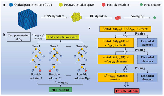
Figure 1.
Process of the LUT element matching algorithm based on RF. (a) Process of obtaining the final solution from the LUT. The blue cubes represent the elements of the LUT, yellow cubes represent the reduced solution space obtained by the k-NN algorithm, red cubes represent the possible solutions after processing by the RF algorithm, and the green circle represents the final solution after averaging the possible solutions. The three cubes belong to the same data set. The circle indicates that it generally does not correspond to any LUT element. (b) Workflow of the RF algorithm. Using the “bagging” strategy to extract several permutations from the full permutation to generate decision trees. Each tree prunes optical parameters according to its permutation. The orange circles represent the elements retained during each pruning, light blue circles represent the excluded parts, and arrows indicate different directions in different dimensions. The red circle is the output of a single decision tree, i.e., a possible solution. After averaging all possible solutions, the final solution is obtained, where the yellow part corresponds to the reduced solution space in (a), and the green part corresponds to the final solution. (c) Pruning process of a single decision tree. For each pruning, the optical parameter distances are first sorted. In the first step, for example, is selected, which means sorting based on the distance of and retaining the top portion with the smallest distances. In the second step, is selected, and the remaining part is sorted and pruned based on the distance of . This process continues until the last pruning, where the remaining part is output as a possible solution.
Using the k-NN algorithm to calculate the differences between the input and LUT parameter sets reduced the possible solution range to a certain interval [43]. Specifically, the implementation involves calculating the Mahalanobis distance [44]:
where is the inverse of the covariance matrix. The k-NN algorithm uses to retain the LUT elements closest to the input data, forming a solution space consisting of elements. This rapidly generated reduced solution space enhances the efficiency of the entire inversion process while encompassing all parameter sets close to the possible solutions.
The RF method was employed to perform weight analysis on all elements within the reduced solution space, combined with the concept of feature pruning to generate a series of possible solutions. An RF is an ensemble of decision trees constructed using randomly chosen criteria [45]. In this approach, the “bagging” strategy was used to extract permutations from the full permutation of 11 optical parameters (11! = 39916800). These permutations serve as the order for the subsequent decision tree pruning (i.e., the number of decision trees generated is ). The “bagging” strategy is a common method of random sampling with replacement, commonly used in constructing RF decision trees. For each decision tree with a specific pruning order, the distance between the optical parameters was calculated as follows:
where subscript is the type of optical parameter that is currently pruned. To facilitate comparisons of distance levels between the optical parameters, relative distances were used instead of absolute distances.
The pruning method is based on the size of , retaining only a portion with smaller distances, with a proportion of (). After pruning all optical parameters, the retained elements have the smallest differences and are stored as possible solutions. After all of the decision trees have made their final outputs, averaging all possible solutions yields the final solution, obtaining CRI () and APSD (, ). Figure 1b illustrates the process of the RF strategy, including the generation of decision trees and the final results. Figure 1c shows the specific pruning process of an individual decision tree.
The inversion of requires an additional step. Since has a proportional change to the aerosol optical parameters, it can be estimated by the mean of the ratio between the input parameters and the original optical parameters (3β + 2α) of the final solution [30]:
where is the original set of optical parameters (3β + 2α).
The selection of , , and the pruning coefficient in k-NN are related to the lidar configuration, LUT, and input data, and it is challenging to find a fixed combination of them that simultaneously achieves optimal computational efficiency and inversion accuracy [30]. It is sufficient to select a relatively suitable set of values that can yield good results for a wide range of data. For the configuration of 3β + 2α, , , can yield a reasonable balance between accuracy and efficiency. This method represents only the basic part of the algorithm, which is referred to as the “basic algorithm” in the following sections. In Section 2.2, the optimization of the strategy generated by RF and the introduction of a self-posed scheme are discussed.
2.2. Retrieval Algorithm for Fine-Mode Aerosol Microphysical Properties Based on LUT—Modified Algorithm: Weighted “Bagging” Strategy and Self-Posed Scheme
The basic algorithm adopts a “bagging” strategy to generate decision trees. To avoid excessive computation time, the number of decision trees is usually set to approximately 500–1000, much smaller than the total number of permutations (11! = 39,916,800). For the “bagging” strategy, when the sampling times increase, the number of samples that are not extracted approaches zero [46]. Therefore, the difference between generated decision trees in each round of sampling is large, which increases the instability of the results. Although the final solution was averaged, the bias caused by the large permutation space could not be avoided. The inversion system is ill-posed because of the insufficient input information, which manifests as discontinuous and non-unique solutions caused by insufficient constraint equations. The principle of the LUT-based inversion method is elemental matching. Owing to the limitations of the data dimensions and system fluctuations, when generating possible solutions as shown in Figure 1c, elements with large differences are included, which affects the accuracy of the inversion. To overcome these issues, this section introduces a modified algorithm that optimizes the “bagging” strategy and adopts a self-posed scheme, including a constraint window and local interpolation. The constraint window replaces the LUT in the second inversion and local interpolation is used to interpolate a selected local region of the LUT.
Figure 2 illustrates the modified algorithm. The algorithm underwent two inversion processes, in which the results of the first inversion served as constraints for the second inversion. The results of the second inversion served as the output for the entire algorithm. We will now explain the weighted “bagging” strategy, constraint windows, and local interpolation in turn.
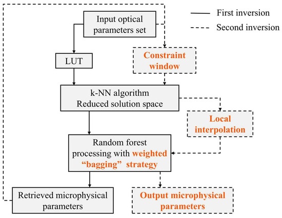
Figure 2.
Process diagram of the modified algorithm. It includes two inversion iterations, where the solid lines depict the process of the first inversion and the dashed lines represent the process of the second inversion. The parts highlighted in orange indicate the additional aspects introduced by the modified algorithm compared to the basic algorithm.
To mitigate the algorithm’s instability and ensure consistent and reasonable criteria for generating each decision tree, a weighted “bagging” strategy was employed. After reducing the solution space using the k-NN algorithm, the relative distances between all elements in the solution space and the input data were calculated using Equation (8). Figure 3a illustrates the distance distribution of the 11 optical parameters generated during a particular algorithm run as an example. There were significant differences in the distance distribution of each optical parameter, with some distances concentrated at smaller values and others dispersed at larger values. Figure 3b shows the mapping of the sixth optical parameter after pruning the second optical parameter. The red-shaded area represents the remaining elements after pruning. The second optical parameter represents concentrated parameters, whereas the sixth optical parameter represents dispersed parameters. Although the elements retained after pruning ensure that the solution space is closer to the input of the second optical parameter, the error in the sixth optical parameter is relatively large, which is detrimental to the inversion. Figure 3c shows the operation that is opposite to the one shown in Figure 3b, in which pruning the sixth optical parameter results in the retained data still having a relatively small distance from the second optical parameter. This phenomenon reveals how randomly generated decision trees produce unstable results. The order of pruning affects the entire inversion process, and the random generation sequence makes this influence uncontrollable, resulting in more divergent results.
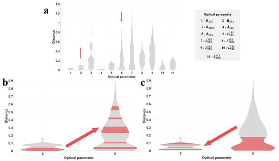
Figure 3.
Example of the decision tree pruning process. (a) Distances between all elements in the reduced solution space and the input optical parameter set on the 11 optical parameters. The horizontal axis represents different optical parameters, and the vertical axis represents the magnitude of the distance. The shaded area in the graph indicates the distribution of the data. Optical parameters corresponding to 1–11 are explained on the right side. (b) Operation’s mapping on the sixth optical parameter when pruning the second optical parameter in (a). The red-shaded area represents the data retained after pruning. (c) Operation’s mapping on the second optical parameter when pruning the sixth optical parameter in (a).
In summary, the results obtained by pruning the optical parameters with greater distance levels are more accurate. This inspired a method of reducing instability, namely, weighted decision tree generation based on the distance between optical parameters. The distances of all the elements in the solution space for the 11 parameters were averaged to represent their distance levels and sorted. The decision-tree pruning order changes from completely random to a pattern in which parameters with largest distance levels are more likely to be selected first and parameters with smallest distance levels are more likely to be selected last. This operation does not eliminate randomness, which is the core idea of the RF method. However, after considering the instability caused by randomness in an overly large space, the results are constrained to a solution space that is favorable in the consequent pruning.
A constraint window is generated based on the results of the first inversion. This constraint window allows us to further constrain the LUT and is applied in a feedback-like manner in the second inversion run, replacing the LUT. The modified algorithm is subjected to two inversions. In the first inversion, the microphysical parameters are obtained and the corresponding optical parameters are calculated using the Mie theory to derive a normalized optical parameter set. By merging the microphysical and optical parameters as inputs, the k-NN algorithm is applied to all LUT elements containing microphysical and optical parameters to generate the constraint window. The generation process of the constraint window is done in a similar fashion to that of the reduced solution space, but with some differences, as shown in Figure 4. The constraint window corresponds to the LUT. In the first inversion, the LUT serves as the entire “map” that is used to search for matching “locations” with the input. In contrast, in the second inversion, the constraint window acts as a “restricted area”, excluding potential non-unique solutions outside this area. The results obtained using the basic algorithm in the first inversion proved to be relatively reliable [31], which is a prerequisite for the application of this approach.

Figure 4.
Flowchart of generating the reduced solution space and the constraint window. The blue portion represents the generation process of the reduced solution space and the green portion represents the generation process of the constraint window.
Local interpolation, also known as the fine-tuning of the local region of the LUT, balances inversion accuracy with computational efficiency. In the LUT method, a special class of input data comprises the grid points of the LUT that precisely match the parameter values of the LUT elements. However, it is highly unlikely that the actual input data will match one of the grid points, leading to inevitable errors. One strategy to overcome the error of non-grid points is to increase the size of the LUT, that is, to generate LUTs with smaller step sizes and larger ranges of microphysical parameters. However, this approach significantly increases the computational cost and is challenging to apply in practical scenarios. This study employs local interpolation as an alternative to fine-tuning the LUT. Owing to the fluctuation and discontinuity of the LUT data, a segmented cubic Hermite interpolation is employed, which ensures the continuity of both the function and its derivative [47]. Interpolating 4-dimensional inputs and 11-dimensional outputs is quite complex. Here, a simple step-by-step approach is presented. First, three of the four inputs were fixed, and all the values of the remaining inputs along with the corresponding outputs were selected. Interpolation was then performed on all 11 outputs, followed by the same process for the other inputs. An interpolation ratio () is defined, with = 2 chosen to balance the interpolation effectiveness and computational load, which implies inserting one point between every two points. Considering the demand for algorithm efficiency in practical applications, local interpolation was applied to the solution space reduced by k-NN in the second inversion.
2.3. Source and Processing of NASA DISCOVER-AQ Field Campaign Data
To evaluate the algorithms mentioned in this paper, we chose NASA’s DISCOVER-AQ field campaign as a case study in view of the availability of high-quality concurrent lidar and in-situ observations. NASA’s HSRL-2 system uses the 3β + 2α configuration, and it is one of the most advanced HSRL systems in the world. The HSRL-2 system has been involved in various field campaigns, including the DISCOVER-AQ field campaign. DISCOVER-AQ was conducted over the course of four years (2011–2014) in four different locations to assess the air quality by combining satellite, airborne, and ground-based measurements [18]. Two aircraft were used during the campaign. The B-200 aircraft carried the HSRL-2 system, flying along a route at an 8.5 km altitude to simulate satellite observations. The flight path of the P-3B aircraft includes several spiral patterns that intersect the flight path of the B-200. The aircraft spiraled up and down from the ground to an altitude of 5 km. A P-3B instrument was used to measure aerosols and trace gases to assess the ambient aerosol properties. The trajectories of both aircraft were coordinated with similar flight times, allowing for a comparison between the HSRL measurements within the P-3B spirals and the in-situ measurements. The study presented in this contribution focuses only on activities in California on 30 and 31 January 2013. The flight paths of the two aircraft are shown in Figure 5.
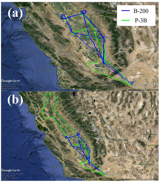
Figure 5.
Aircraft trajectory maps in California on (a) 30 January and (b) 31 January. The blue trace represents the track of the B-200 and the green trace represents that of the P-3B.
In the following we briefly introduce the HSRL-2 system with the detailed descriptions available in the literature [48]. The HSRL-2 system measures the aerosol backscatter coefficient (β) and depolarization ratio (δ) at 355, 532, and 1064 nm [49], as well as the aerosol extinction coefficient (α) at 355 and 532 nm [50]. These data allow us to calculate additional data products such as the Ångström exponent and aerosol optical thickness. The HSRL-2 system samples at a temporal frequency of 2 Hz and a spatial resolution of 15 m, followed by horizontal averaging over 10 s (for β and δ) and 60 s (for α), corresponding to spatial resolutions of 1 and 6 km at the nominal aircraft speed. Considering the limitations of the Mie theory for spherical particles, only points with particle depolarization ratios at 532 nm of are used for inversion. Furthermore, data points outside the range of Ångström exponent of [1.5, 2.5] are excluded, as this value range represents the typical characteristics of fine-mode aerosol particles [51,52].
The other aircraft, P-3B, conducted in-situ measurements of aerosols, including APSD, aerosol scattering coefficients, and absorption coefficients. The Ultra-High Sensitivity Aerosol Spectrometer (UHSAS) measures the APSD in the diameter range of 0.06 to 1 μm, mainly capturing information about fine-mode aerosol particles. Coarse-mode aerosol particles were sampled using a Laser Aerosol Spectrometer (LAS) to measure particles with a diameter range of 0.09 to 7.5 μm. To ensure the absence of coarse-mode particles in the UHSAS measurements, points with () were excluded from our data analysis.
Generally, in-situ measurements are conducted under dry conditions (Relative Humidity, RH < 20%), whereas HSRL measurements are conducted under ambient RH conditions [53]. However, aerosols can absorb moisture under high RH conditions, which affects their physical properties. Therefore, measurements from in-situ instruments cannot represent the true measurements in the atmosphere, which is one of the major limitations in the validation of lidar measurements with in-situ measurements [52]. To overcome this limitation, a humidity correction was applied to the in-situ measurements on P-3B for the scattering coefficient. The scattering coefficients under dry and wet conditions (550 nm) were measured using a pair of integrating nephelometers, and the Ångström exponent was used to adjust the wavelength from 550 nm to 532 nm [18]. One nephelometer operated at a low RH ( ~ 10%), while the other operated at a high RH ( ~ 80–85%). This allows the calculation of aerosol hygroscopicity, :
where and are the scattering coefficients measured under and , respectively. An open-path diode laser hygrometer was used to measure the static temperature and water vapor concentration, which could be used to derive the ambient relative humidity [54]. Based on the hygroscopicity , the scattering coefficients under dry conditions can be corrected:
The dry aerosol absorption coefficient was determined at 532 nm using a Particle Soot Absorption Photometer (PSAP). The impact of hygroscopic growth on the absorption coefficient was neglected. The aerosol extinction coefficient in the real atmosphere is the sum of the hygroscopicity-corrected scattering coefficient and dry absorption coefficient.
Figure 6 illustrates the data processing approach used for the DISCOVER-AQ field campaign. Because of the 15 km separation limit between the two aircraft, the HSRL data were averaged vertically across 75 m height bins and temporally over 1.5 min. The diameter of the P-3B spirals was 6–10 km, with a vertical resolution of 5 m and a temporal resolution of 1 s, thus requiring the same averaging of the P-3B data to match the resolution of the HSRL data.
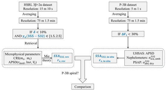
Figure 6.
Data processing and comparison process between the two aircraft. The blue annotations indicate important parameters and results during the process. HSRL optical data undergoes screening for depolarization ratio () and Ångström exponent (), followed by inversion to obtain CRI and APSD, and then the calculation of , , and products. P-3B data were screened based on , and APSD, environmental scattering coefficient, and dry absorption coefficient were obtained from measurements by UHSAS, nephelometer, and PSAP, respectively. Finally, , , and are computed. The conditions for mutual comparison of the products obtained from both aircraft are within the spirals of P-3B, where validation of the aerosol vertical profile information can be performed.
3. Results
This section presents the tests and demonstrates the results and analyses of the algorithms described in Section 2. Section 3.1, Section 3.2 and Section 3.3 focus on the numerical simulation test of the algorithm, with Section 3.1 focusing on an error-free input test and Section 3.2 and Section 3.3 examining the algorithm’s performance with input errors. Section 3.4 applies the algorithms to the DISCOVER-AQ scenario in a real-world setting.
3.1. Numerical Test of Simulated Error-Free Data
In addition to the 3β + 2α configuration, this study investigated three other configurations: 3β + 1α, 2β + 1α, and 3β. The reason for this is that instruments for measuring the extinction coefficient at 355 nm are complex and expensive, and thus the 3β + 2α configuration is difficult to implement in many lidar systems. Commonly, simpler instruments lack backscatter or extinction measurements. A large amount of simulated error-free data was used to test the performance of these algorithms. To study the impact of input data on inversion performance, the simulated input types were divided into two categories: grid points and non-grid points. Grid points refer to data points whose parameter values exactly match those of the elements in the LUT, whereas non-grid points do not. The test on the grid points shows the greatest performance of the algorithm; in other words, the input case that is likely to get the most accurate result. Tests on non-grid points represent performance in general. The range of the simulated error-free data was narrower than that of the LUT. More detailed information on the input data is provided in Table 2. Simulated data generation was on the condition of .

Table 2.
Microphysical parameters for error-free input data. The data are divided into two types for algorithm testing: (1) Grid points refer to data points whose parameter values exactly match those of elements in the LUT (Grid) and (2) Non-grid points refer to data points whose parameter value do not overlay any elements in the LUT (Non-grid).
To validate the effectiveness of the improvement strategy, the basic and modified algorithms were employed to simulate the same set of error-free data. The results obtained directly from the LUT by the algorithms include , , , and . Based on the Mie scattering theory, can be calculated and and can be derived using Equations (3) and (9). Therefore, the final results consist of errors in five parameters: , , , , and , where the first three are represented in absolute values and the last two in relative values [24,25,30]. We defined:
The subscript “retrieved” denotes the results obtained from the inversion, while the subscript “true” represents the true values. The algorithms were executed on a personal computer with an AMD Ryzen 7 4800H processor running MATLAB 2023a. The times required by both the basic and modified algorithms were recorded to evaluate the efficiency lost by the modified algorithm.
The inversion results for the four lidar configurations are shown in Figure 7a–e,g–k and Figure 8a–e,g–k. The bar charts depict the average inversion errors of the test dataset. The errors on grid points were significantly smaller than those on non-grid points because the LUT method theoretically cannot obtain the most accurate solution for non-grid points. The 3β + 2α configuration exhibited the smallest error, followed by 3β + 1α, 2β + 1α, and 3β. This outcome is attributed to the maximum information content of 3β + 2α, which has 11 normalized optical parameters, whereas the others have 6, 4, and 3 normalized optical parameters, respectively, leading to an increase in errors as the information content decreases. The modified algorithm significantly enhanced inversion accuracy, especially for grid point data. The errors on the grid points for 3β + 2α and 3β + 1α were almost negligible and those for 2β + 1α and 3β were substantially reduced. For non-grid point data, the errors for 3β + 2α, 3β + 1α, and 2β + 1α are notably reduced, resulting in similar average error levels. The non-grid inversion errors of the modified algorithm for 3β + 2α, 3β + 1α, and 2β + 1α were reduced on average to 41%, 30%, and 32% of those of the basic algorithm, respectively. For the 3β configuration, the performance improvement of the modified algorithm on non-grid points was not significant, with almost no improvement. This may be due to the extreme nature of the 3β configuration, which has only 3 normalized optical parameters, resulting in insufficient information from a system of strong ill-posedness. The testing of 3β serves as a lower limit test for the algorithm, as actual lidar systems require at least one extinction measurement to ensure the inversion of aerosol microphysical parameters [55]. The above analysis demonstrated the effectiveness of the modified algorithm strategy for overcoming the ill-posedness of inversion systems and narrowing the gap in error levels between different lidar configurations. However, this does not imply that complex configurations do not contribute to an improvement in accuracy. Due to the limited test data, the results of these configurations serve only as references, demonstrating that under the modified algorithm, simple configurations can achieve results comparable to those of complex configurations within a certain range.
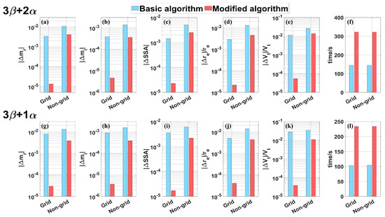
Figure 7.
Average retrieval errors and computation time for the microphysical parameters under the 3β + 2α and 3β + 1α configurations. (a–f) The retrieval errors and consumed time for 3β + 2α. (g–l) The retrieval errors and consumed time for 3β + 1α. The blue bars represent the results of the basic algorithm, while the red bars represent the results of the modified algorithm. The test data are divided into two categories: grid points and non−grid points.
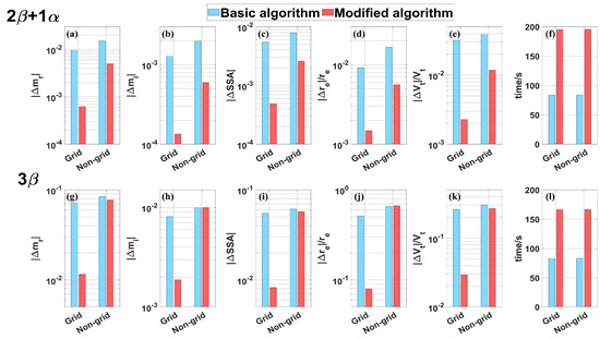
Figure 8.
Average retrieval errors and computation time for the microphysical parameters under the 2β + 1α and 3β configurations. (a–f) The retrieval errors and consumed time for 2β + 1α. (g–l) The retrieval errors and consumed time for 3β. The results are marked similarly to those in Figure 7.
Figure 7f,l and Figure 8f,l depict the time consumed by the basic and modified algorithms to invert these data points using the same computer hardware and MATLAB 2023aconditions. Overall, the time consumed by the algorithms was, in the order from longest to shortest, 3β + 2α, 3β + 1α, 2β + 1α, and 3β. This was influenced by the difference in information content; the greater the number of optical parameters, the more dimensions the RF algorithm needs to prune and the longer the interpolation program run time. The time required for the grid and non-grid points was almost the same because the computational load of the system remained the same, regardless of whether the input precisely matched the elements of the LUT. The modified algorithm required approximately twice the time of the basic algorithm, which is the cost of the accuracy improvement. However, the time required is still within an acceptable range.
In addition, to test the improvement of the retrieval stability caused by the modified algorithm, both the basic and modified algorithms were run 100 times for each lidar configuration on the same dataset. The results are shown in Figure 9 and Figure 10. Box plots were generated using the InterQuartile Range (IQR) strategy. The upper and lower sides of the rectangle represent the 25th and 75th percentiles, the middle line represents the median, and the bottom and top lines represent the minimum and maximum values, respectively [56]. It is evident that for all configurations, the modified algorithm significantly enhanced the stability of the inversion. This result demonstrates that the basic algorithm’s “bagging” strategy indeed introduces excessive randomness, leading to significant differences in the inversion results for the same data each time. The weighted “bagging” strategy to some extent reduces the randomness, making the algorithm more stable.
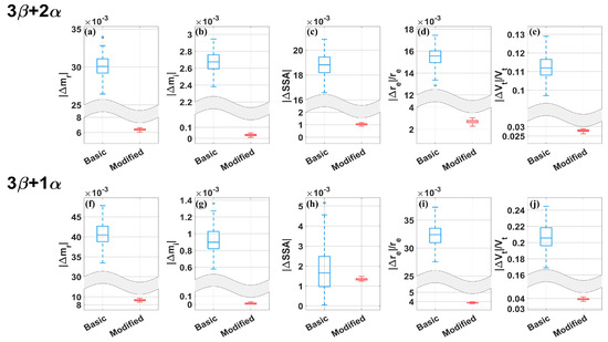
Figure 9.
Stability testing results for the retrieval algorithms under the 3β + 2α and 3β + 1α configurations. (a–e) Box plots for retrieval errors of aerosol microphysical properties under 3β + 2α. (f–j) Box plots for retrieval errors of aerosol microphysical properties under 3β + 1α. The box plots are generated according to the IQR strategy. The blue box plots represent the basic algorithm and the red plots represent the modified algorithm. The wavy−shaded areas on the y−axis indicate truncation and jumps for visualization purposes.
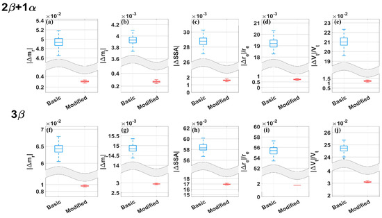
Figure 10.
Stability testing results for the retrieval algorithms under the 2β + 1α and 3β configurations. (a–e) Box plots for retrieval errors of aerosol microphysical properties under 2β + 1α. (f–j) Box plots for retrieval errors of aerosol microphysical properties under 3β. The meaning of the labels is consistent with Figure 9.
3.2. Sensitivity Study of Individual Input Optical Property
Research on regularization methods has shown that inversion errors are linearly related to optical data errors [57]. To explore this relationship in our method, we artificially introduced distortions into the individual input optical properties. Currently, the measurement uncertainty of most lidar systems is within ±20% [58]. Therefore, in studying the influence of individual input optical property on the inversion results, fixed errors of 0%, ±10%, and ±20% were used. The simulated non-grid data from Table 2 were used. This method involved artificially distorting an individual optical property obtained from the Mie theory calculations for each simulation. Sensitivity studies of the fixed errors were conducted separately for each optical property under the same lidar configuration. Only the modified algorithm was used in this section.
The results are presented as functions of the inversion error versus the fixed error in Figure 11. In many cases, the inversion error was approximately linearly related to the fixed error. However, the linear relationship did not always exist, for example, the inversion of showed an axisymmetric linear relationship, and was always overestimated. In the inversion of , the relation between the input error of and the inversion error was nonlinear, and it was more sensitive to the negative error. Many similar abnormal relationships were shown in Figure 11.
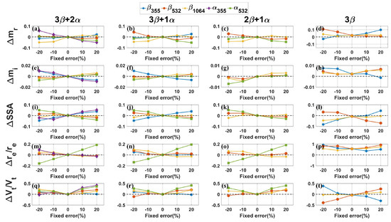
Figure 11.
Function of inversion error versus fixed error when artificially distorting individual input optical properties. (a–d) Inversion errors of 3β + 2α (a), 3β + 1α (b), 2β + 1α (c) and 3β (d) configurations regarding . (e–h) Same as (a–d), but showing inversion errors regarding . (i–l) Same as (a–d), but showing inversion errors regarding . (m–p) Same as (a–d), but showing inversion errors regarding . (q–t) Same as (a–d), but showing inversion errors regarding . The horizontal axis represents the value of the fixed error, while the vertical axis represents the inversion error, with the zero−error line highlighted by a dashed line. For different optical parameters, lines with different colors and markers represent , , and with blue hexagons, orange circles, and yellow stars, respectively, while and are represented by purple diamonds and green squares, respectively.
For the 3β + 2α configuration, had the greatest impact on the inversion results for , followed by , while the other optical properties had less influence. The inversion of was the most sensitive to and , followed by , with and being the least sensitive. The inversion of , which integrates and , was most affected by , , and , as shown in Figure 11i. The retrieval of was highly sensitive to , followed by . In the inversion of , the results showed an approximately symmetric linear relationship around the zero-error point, with a clear overestimation regardless of the sign of the fixed error, which is consistent with previous studies [28]. The inversion results for were most sensitive to and , and least sensitive to . Overall, the two extinction properties played the most important role in the inversion of 3β + 2α, while the backscatter properties had a significant impact on the inversion of some aerosol microphysical parameters.
The results for 3β + 1α and 2β + 1α were similar to those for 3β + 2α. Notably, in Figure 11b, the inversion of is more sensitive to than in Figure 11a. The curves and trends in 3β + 1α and 2β + 1α with existing channels were generally consistent with those in 3β + 2α. A comparison of the results of these three configurations demonstrated that the absence of a few optical properties did not significantly affect the quality of the inversion results in the modified algorithm. Combined with the results from Section 3.1, this further demonstrates that the modified algorithm has a higher tolerance for simple lidar configurations.
The results for 3β showed some differences from the above conclusions, such as higher sensitivity to the backscatter properties and significant overestimation in , , and , with particularly poor performance in the inversion of . This phenomenon can be explained by the lack of the most important extinction properties in 3β, as relying solely on the information provided by backscatter properties is insufficient for successful inversions. The comparison with the results for 2β + 1α corroborates this conclusion, demonstrating the indispensable role of extinction properties in the inversion of aerosol microphysical parameters.
3.3. Study on Input Optical Properties with Random Gaussian Noise
The signal noise generated by actual lidar systems clearly does not appear only in the individual optical properties. Each optical property can have different errors. To evaluate the performance of the algorithm in real systems, Gaussian noise generated according to the uncertainty of the actual lidar systems was applied to the microphysical parameters listed in Table 2. As in previous studies [31], if the error level of Gaussian noise is denoted as x%, it means that this value is the same as the 3-σ value of the Gaussian distribution (i.e., the geometric standard deviation σ = x/3). Gaussian noise was applied with error levels of 10% and 20%. To avoid significant randomness, 100 inversion repetitions were performed for each input, with random noise generated independently each time. This test section applies only to the modified algorithm.
To illustrate the distribution of the data more intuitively, violin plots, which are enhanced versions of box plots that display the probability density of the data, were used to describe the results [59].
Almost all data distributions approximately followed a Gaussian distribution, except for the inversion of and in the 3β configuration as shown in Figure 12p,t. All configurations exhibited varying degrees of overestimation in the inversion of , where the green bars were significantly higher than the white dots, corresponding to previous analyses. However, in all other subpanels, the mean and zero points were very close. There were no significant differences among the results of 3β + 2α, 3β + 1α, and 2β + 1α. In Figure 12o,s, the performance of the inversion of and in the 2β + 1α configuration is the best, with the data being more concentrated. This is a positive phenomenon, once again demonstrating the improvement in the accuracy of microphysical parameter inversion by the modified algorithm for simple lidar configurations; it is expected to make the lack of optical channels no longer the most fatal flaw in lidar systems. The performance of 3β was relatively poor.
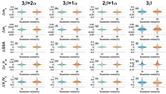
Figure 12.
Inversion errors after applying random Gaussian noise disturbance to the input data at error levels of 10% and 20%. (a–d) Inversion errors of 3β + 2α (a), 3β + 1α (b), 2β + 1α (c) and 3β (d) configurations regarding . (e–h) Same as (a–d), but showing inversion errors regarding . (i–l) Same as (a–d), but showing inversion errors regarding . (m–p) Same as (a–d), but showing inversion errors regarding . (q–t) Same as (a–d), but showing inversion errors regarding . The error levels of 10% and 20% are represented by blue and orange images, respectively. The results are presented in the form of violin plots, which are an enhanced version of box plots that provide more detailed information about the distribution of the data. In each violin plot, the vertical gray bars correspond to the ends of the box plot whiskers, representing the maximum and minimum values of the statistical distribution. The shaded area corresponds to the interquartile range of 25% and 75% of the box plot. Horizontally, the shaded area represents the probability density function of the data distribution, showing the frequency of data distribution in each interval. The white points indicate the position of zero, and the horizontal green bars represent the mean values.
In real situations, inversions that are too extreme are usually excluded. Therefore, data within the 25th and 75th percentiles can approximate the uncertainty of the inversion, that is, the range of the shaded area. The inversion of CRI and showed less variation as the level of Gaussian noise increased, indicating a higher tolerance for noise, while and were more sensitive to noise, with the distribution of 20% Gaussian noise being more dispersed than that of 10%. 2β + 1α still performed the best in the inversion of and . The explanation for this result is that the test is only a small dataset and the results have a certain degree of occasionality, which makes the performance of 2β + 1α better than other configurations in some aspects. Overall, except for 3β, the uncertainties of the inversion of the other three configurations were not significantly different and relatively small, thus allowing for high-quality inversion results.
3.4. DISCOVER-AQ Case Study
Section 3.1, Section 3.2 and Section 3.3 of the simulated data tests preliminarily demonstrated the comprehensive improvement of the inversion results by the modified algorithm under ideal conditions, as well as the sensitivity in regard to erroneous input data. This demonstrates the theoretical feasibility of the proposed algorithm. However, another necessary process for verifying the algorithm is conducting case studies that directly address various complex uncertainties in real situations. In this section, the modified algorithm was applied to the data obtained during the DISCOVER-AQ field campaign, as introduced in Section 2.3.
The HSRL-2 system carried by the B-200 aircraft provides optical parameters for inversion, including the backscatter coefficient, extinction coefficient, depolarization ratio, and Ångström exponent. The P-3B aircraft was equipped with multiple in-situ instruments to measure environmental aerosol particles and obtain aerosol and APSD data. The flight path of the P-3B includes many spiral points. At each location, the aircraft ascends or descends at a constant speed; therefore, the aerosol profile information of that location can be used as validation data for lidar inversion. Activities in California on 30 and 31 January 2013 were selected for the study. The flight paths on these two days were almost identical, except for one circuit of P-3B (highlighted by the green trajectory in Figure 5b). There were six spiral points for P-3B, and the inversion results at these six validation points were verified. The latitude and longitude information of the six validation points are shown in Table 3.

Table 3.
Latitude and longitude information of P-3B six spiral points.
Figure 13 provides the raw optical data obtained by HSRL on 30 and 31 January, including five optical parameters (, , , , and ) and the Ångstrom exponent . The flight paths of the B-200 aircraft were almost identical on both days. Comparing the optical parameter profiles for the two days, it can be observed that the aerosol layer on January 31st was slightly lower than the previous day, as indicated by the lower altitude of the boundary of the data (dark blue region). However, the overall temporal trend remained similar, indicating a relative decrease in the aerosol layer over the course of the day. Moreover, the temporal and height continuities of the profiles were good, indicating a uniform composition of the aerosol layer. It is noteworthy that mostly varied between 1.5 and 2.5, especially at relatively lower altitudes, which is consistent with the typical characteristics of fine-mode aerosol particles. This result provides favorable conditions for the application of the modified algorithm.
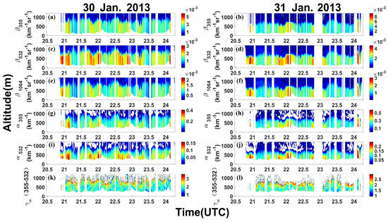
Figure 13.
Original optical data from the HSRL collected during the DISCOVER−AQ field campaign in California on 30 and 31 January 2013. The horizontal axis represents UTC time, and the vertical axis represents altitude above sea level. The data for the two days are shown in the left and right columns, respectively. (a,b) Profile s of on the two days. (c,d) Profile s of on the two days. (e,f) Profile s of on the two days. (g,h) Profile s of on the two days. (i,j) Profile s of on the two days. (k,l) Profile s of on the two days.
Figure 14 and Figure 15 show the results obtained on 30 and 31 January, respectively, following the process outlined in Figure 6.
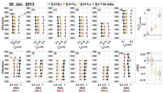
Figure 14.
Comparisons of retrieved microphysical parameter profiles from the HSRL on 30 January 2013, with P−3B in-situ measurements at six validation sites. (a–g) represent the results for , while (h–n) represent the results for . (a–f) and (h–m) show the profile information for and , respectively, at the six sites. The results retrieved using the 3β + 2α, 3β + 1α, 2β + 1α, and 3β configurations are depicted with blue, orange, yellow, and purple lines and markers, respectively, while in-situ measurement data are represented by black lines and markers. The x-axis represents the values of the microphysical parameters, and the y-axis represents altitude. (g,n) show box plots of the retrieval errors for all data points at the six validation sites on that day, where the color scheme matches that of Figure 9.
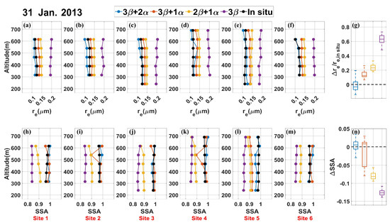
Figure 15.
Comparisons of retrieved microphysical parameter profiles from the HSRL on 31 January 2013, with P-3B in-situ measurements at six validation sites. (a–g) represent the results for , while (h–n) represent the results for . (a–f) and (h–m) show the profile information for and , respectively, at the six sites. The annotations in the figure correspond to those in Figure 14.
The profiles of the inversion results of were comparably stable in altitude for almost all configurations. The exception to this result was the case of 3β in the 700–800 m height range in Figure 14a. We also found minor fluctuations for 3β + 2α in the 500–600 m height range in Figure 15d. This result indicated the high stability of the modified algorithm for the APSD retrievals. Overall, the 3β + 2α configuration showed the best agreement with the in-situ measurement data, without significant overestimation or underestimation, whereas the other configurations exhibited clear overestimation. The 3β configuration yielded the largest errors, with the median inversion error reaching 85% (as shown in Figure 14g), compared to 6%, 26%, and 39% for 3β + 2α, 3β + 1α, and 2β + 1α, respectively. Although the average inversion error for 3β + 2α was the smallest (as shown in Figure 15g), some points exhibited higher errors than 3β + 1α, indicating slightly lower stability compared to 3β + 1α and 2β + 1α. In summary, 3β + 2α and 3β + 1α were relatively reliable for retrieval, while 2β + 1α was comparable to 3β + 1α in some cases but performed poorly overall. The results we obtained for the 3β configuration showed the lowest quality and can hardly be used.
Regarding the retrieval results, significant discontinuities were observed at several points in the profiles. retrieval depends largely on the retrieval results of , and the above analysis indicates the good stability of the APSD retrieval results. This suggests that the modified algorithm was more sensitive to retrieval than to APSD retrieval, leading to instability in retrieval. However, most of these significant instabilities were observed in the 3β + 1α configuration, while the results for other configurations were relatively stable. The profiles demonstrated that 3β + 2α remained the closest to the in-situ measurements, while 2β + 1α and 3β performed the worst. Surprisingly, despite some instability, the inversion results for 3β + 1α were close to or even surpassed those of 3β + 2α in many data points. Figure 14n and Figure 15n confirm this observation, with the median inversion errors for 3β + 2α (0.012 and 0.005) and 3β + 1α (0.009 and 0.008) being significantly higher than those for 2β + 1α (−0.087 and −0.081) and 3β (−0.100 and −0.126). Therefore, it can be concluded that 3β + 2α and 3β + 1α are relatively reliable for (or ) retrieval but the latter requires handling of some obvious outliers.
Furthermore, we compare the performance of the FAST algorithm in DISCOVER-AQ field campaign with modified algorithm in this study. In the literature [31], the median inversion errors of in the application scenario of the FAST algorithm for 3β + 2α, 3β + 1α, and 2β + 1α are 3.53%, 11.68%, and 12.33% respectively. The median inversion errors of for 3β + 2α, 3β + 1α, and 2β + 1α are 0.010, 0.014, and 0.016, respectively. For 3β + 2α and 3β + 1α, compared with the FAST algorithm, the modified algorithm has significant advantages in the inversion of and similar performance in the inversion of . For 2β + 1α, the modified algorithm is inferior to the FAST algorithm. The reason of this may be because for 2β + 1α, the two inversion processes amplify the complex noise and errors of the actual situation.
Based on extensive validation data, the above analysis preliminarily demonstrated the feasibility of the modified algorithm. Among the six different validation sites, the retrieval performance of 3β + 2α was excellent, followed by that of 3β + 1α, which exhibited outstanding performance in retrieval. 2β + 1α performed relatively poorly and 3β performed the worst. The retrieval of was more stable than that of , which may be due to the weaker HSRL backscatter signal compared to the extinction channels, as demonstrated in Section 3.2. In the case study, inversions were performed for both scenarios. Under the same hardware and software conditions (as mentioned in Section 3.1), the inversion time for the 30 January scenario was 22 min and that for the 31 January scenario was 16 min. Notably, these results were obtained using a personal laptop, and the inversion time could be significantly reduced by using a more powerful computer.
4. Discussion and Conclusions
This study proposed an LUT-based method for retrieving microphysical properties, aiming to reduce the ill-posedness of the retrieval system and improve the accuracy and stability. Building upon previous research, this study introduced a weighted “bagging” strategy and a self-posed strategy, including a constraint window and local interpolation, into the algorithm, resulting in the modified algorithm. The modified algorithm exhibited remarkable performance, with retrieval errors at LUT grid points almost reduced to zero and reductions of 41%, 30%, and 32% in retrieval errors at non-grid points compared to the basic algorithm under 3β + 2α, 3β + 1α, and 2β + 1α configurations, respectively. Both ideal input and error input studies demonstrated that the retrieval performance and sensitivity to noise of 3β + 2α, 3β+1α, and 2β + 1α were at a similar level.
The modified algorithm was applied to case studies of two scenarios from NASA’s DISCOVER-AQ field campaign, where the profiles retrieved from HSRL data were compared with in-situ measurements. The application of the modified algorithm was successful, with the median relative errors in the retrieval of for 3β + 2α being 6% and −3%, for 3β + 1α being 26% and 12%, and for 2β + 1α being 39% and 23% for the two scenarios, respectively. The median absolute errors in retrieval for 3β + 2α were 0.012 and 0.005, for 3β + 1α were 0.009 and 0.008, and for 2β + 1α were −0.087 and −0.081.
Analysis of the results indicated that the modified algorithm effectively mitigates the ill-posedness of the retrieval system and enhances its stability. This study also demonstrated the importance of adding extinction coefficient detection channels, such as Raman channels or hyperspectral resolution channels, to lidars. Furthermore, the investigation of LUT methods revealed the relationship between LUT construction and retrieval results, which may assist with more LUT-based retrieval methods in the future.
This study represents a further attempt at developing unsupervised retrieval methods with a scope limited to fine-mode aerosol particles, thus imposing certain constraints on practical applications. Future research should explore retrievals involving coarse-mode particles. Lastly, the introduction of a feedback mechanism in the modified algorithm through a second retrieval increased the number of hyperparameters such as , , , etc. Too many hyperparameters can significantly impact the system, with minor variations in the combination of hyperparameters potentially leading to drastic changes in the results. Although this study has not yet reached this stage, the increase in hyperparameters poses challenges for algorithm debugging and potential risks that need to be addressed in future optimizations.
Author Contributions
Conceptualization, Z.Z. and Y.M.; methodology, Z.Z., Y.M. and Z.Y.; software, Z.Z.; validation, Z.Z. and Z.Y.; formal analysis, Z.Z., Y.M. and Z.Y.; investigation, Z.Z.; resources, Y.M., Z.Y., Q.H., I.V., D.M. and W.G.; data curation, Z.Z.; writing—original draft preparation, Z.Z. and Z.Y.; writing—review and editing, Z.Z., Y.M., Z.Y., Q.H., I.V. and D.M.; visualization, Z.Z., Y.M. and Z.Y.; supervision, Y.M. and Z.Y.; project administration, Y.M. and Z.Y.; funding acquisition, Y.M., Z.Y. and W.G. All authors have read and agreed to the published version of the manuscript.
Funding
This research was funded by the National Key Research and Development Program of China (Grant No. 2023YFC3007802 and No. 2023YFC3007803), the National Natural Science Foundation of China (Grant No. 42071348 and No. 42205130) and the National Key Research and Development in Hubei Province (Grant No. 2021BCA220).
Data Availability Statement
The data from the DISCOVER-AQ used in this study can be found in https://www-air.larc.nasa.gov/missions/discover-aq/discover-aq.html (accessed on 1 December 2010).
Acknowledgments
The authors thank the science team from NASA Langley Center for providing the open-accessed data during the DISCOVER-AQ field campaign and the State Key Laboratory of Modern Optical Instrumentation, College of Optical Science and Engineering, Zhejiang University for publishing new method that stimulates inspiration for this work. The authors acknowledge the support of State Key Laboratory of Information Engineering in Surveying, Mapping and Remote Sensing and School of Remote Sensing and Information Engineering, Wuhan University.
Conflicts of Interest
The authors declare no conflicts of interest.
References
- Ali, M.A.; Huang, Z.W.; Bilal, M.; Assiri, M.E.; Mhawish, A.; Nichol, J.E.; de Leeuw, G.; Almazroui, M.; Wang, Y.; Alsubhi, Y. Long-term PM2.5 pollution over China: Identification of PM2.5 pollution hotspots and source contributions. Sci. Total Environ. Environ. 2023, 893, 164871. [Google Scholar] [CrossRef] [PubMed]
- Lee, K.H.; Kim, Y.J.; Kim, M.J. Characteristics of aerosol observed during two severe haze events over Korea in June and October 2004. Atmos. Environ. 2006, 40, 5146–5155. [Google Scholar] [CrossRef]
- Penner, J.E.; Dickinson, R.E.; Oneill, C.A. Effects of Aerosol from Biomass Burning on the Global Radiation Budget. Science 1992, 256, 1432–1434. [Google Scholar] [CrossRef] [PubMed]
- Solomon, S.; Qin, D.; Manning, M.R.; Chen, Z.; Marquis, M.; Averyt, K.; Tignor, M.M.B.; Miller, H.L. Climate Change 2007: The Physical Science Basis. Contribution of Working Group I to the Fourth Assessment Report of the Intergovernmental Panel on Climate Change; Cambridge University Press: Cambridge, UK, 2007. [Google Scholar]
- Torres, B.; Dubovik, O.; Fuertes, D.; Schuster, G.; Cachorro, V.E.; Lapyonok, T.; Goloub, P.; Blarel, L.; Barreto, A.; Mallet, M.; et al. Advanced characterisation of aerosol size properties from measurements of spectral optical depth using the GRASP algorithm. Atmos. Meas. Tech. 2017, 10, 3743–3781. [Google Scholar] [CrossRef] [PubMed]
- Yan, X.; Zang, Z.; Zhao, C.F.; Husi, L. Understanding global changes in fine-mode aerosols during 2008–2017 using statistical methods and deep learning approach. Environ. Int. 2021, 149, 106392. [Google Scholar] [CrossRef] [PubMed]
- Jerrett, M. ATMOSPHERIC SCIENCE The death toll from air-pollution sources. Nature 2015, 525, 330–331. [Google Scholar] [CrossRef] [PubMed]
- Lelieveld, J.; Evans, J.S.; Fnais, M.; Giannadaki, D.; Pozzer, A. The contribution of outdoor air pollution sources to premature mortality on a global scale. Nature 2015, 525, 367–371. [Google Scholar] [CrossRef] [PubMed]
- Ma, Y.Y.; Zhang, M.; Jin, S.K.; Gong, W.; Chen, N.; Chen, Z.Y.; Jin, Y.B.; Shi, Y.F. Long-Term Investigation of Aerosol Optical and Radiative Characteristics in a Typical Megacity of Central China During Winter Haze Periods. J. Geophys. Res.-Atmos. 2019, 124, 12093–12106. [Google Scholar] [CrossRef]
- Di, H.G.; Wang, Q.Y.; Hua, H.B.; Li, S.W.; Yan, Q.; Liu, J.J.; Song, Y.H.; Hua, D.X. Aerosol Microphysical Particle Parameter Inversion and Error Analysis Based on Remote Sensing Data. Remote Sens. 2018, 10, 1753. [Google Scholar] [CrossRef]
- Müller, D.; Wandinger, U.; Ansmann, A. Microphysical particle parameters from extinction and backscatter lidar data by inversion with regularization:: Theory. Appl. Opt. 1999, 38, 2346–2357. [Google Scholar] [CrossRef]
- Zhou, X.W.; Zhou, T.; Fang, S.Y.; Han, B.S.; He, Q. Investigation of the Vertical Distribution Characteristics and Microphysical Properties of Summer Mineral Dust Masses over the Taklimakan Desert Using an Unmanned Aerial Vehicle. Remote Sens. 2023, 15, 3556. [Google Scholar] [CrossRef]
- Kolgotin, A.; Müller, D.; Korenskiy, M.; Veselovskii, I. ORACLES Campaign, September 2016: Inversion of HSRL-2 Observations with Regularization Algorithm into Particle Microphysical Parameters and Comparison to Airborne In-Situ Data. Atmosphere 2023, 14, 1661. [Google Scholar] [CrossRef]
- Wang, L.; Yin, Z.; Lu, T.; Yi, Y.; Dong, X.; Dai, Y.; Bu, Z.; Chen, Y.; Wang, X. 1064 nm rotational Raman polarization lidar for profiling aerosol and cloud characteristics. Opt. Express 2024, 32, 14963–14977. [Google Scholar] [CrossRef]
- Wang, A.; Yin, Z.; Mao, S.; Wang, L.; Yi, Y.; Chen, Q.; Mueller, D.; Wang, X. Measurements of particle extinction coefficients at 1064 nm with lidar: Temperature dependence of rotational Raman channels. Opt. Express 2024, 32, 4650–4667. [Google Scholar] [CrossRef]
- Crumeyrolle, S.; Chen, G.; Ziemba, L.; Beyersdorf, A.; Thornhill, L.; Winstead, E.; Moore, R.H.; Shook, M.A.; Hudgins, C.; Anderson, B.E. Factors that influence surface PM2.5 values inferred from satellite observations: Perspective gained for the US Baltimore-Washington metropolitan area during DISCOVER-AQ. Atmos. Chem. Phys. 2014, 14, 2139–2153. [Google Scholar] [CrossRef]
- Müller, D.; Hostetler, C.A.; Ferrare, R.A.; Burton, S.P.; Chemyakin, E.; Kolgotin, A.; Hair, J.W.; Cook, A.L.; Harper, D.B.; Rogers, R.R.; et al. Airborne Multiwavelength High Spectral Resolution Lidar (HSRL-2) observations during TCAP 2012: Vertical profiles of optical and microphysical properties of a smoke/urban haze plume over the northeastern coast of the US. Atmos. Meas. Tech. 2014, 7, 3487–3496. [Google Scholar] [CrossRef]
- Sawamura, P.; Moore, R.H.; Burton, S.P.; Chemyakin, E.; Müller, D.; Kolgotin, A.; Ferrare, R.A.; Hostetler, C.A.; Ziemba, L.D.; Beyersdorf, A.J.; et al. HSRL-2 aerosol optical measurements and microphysical retrievals vs. airborne in situ measurements during DISCOVER-AQ 2013: An intercomparison study. Atmos. Chem. Phys. 2017, 17, 7229–7243. [Google Scholar]
- Burton, S.P.; Hostetler, C.A.; Cook, A.L.; Hair, J.W.; Seaman, S.T.; Scola, S.; Harper, D.B.; Smith, J.A.; Fenn, M.A.; Ferrare, R.A.; et al. Calibration of a high spectral resolution lidar using a Michelson interferometer, with data examples from ORACLES. Appl. Opt. 2018, 57, 6061–6075. [Google Scholar] [CrossRef]
- Liu, D.; Zheng, Z.F.; Chen, W.B.; Wang, Z.B.; Li, W.J.; Ke, J.; Zhang, Y.P.; Chen, S.J.; Cheng, C.H.; Wang, S.B. Performance estimation of space-borne high-spectral-resolution lidar for cloud and aerosol optical properties at 532 nm. Opt. Express 2019, 27, A481–A494. [Google Scholar] [CrossRef]
- Veselovskii, I.; Dubovik, O.; Kolgotin, A.; Korenskiy, M.; Whiteman, D.N.; Allakhverdiev, K.; Huseyinoglu, F. Linear estimation of particle bulk parameters from multi-wavelength lidar measurements. Atmos. Meas. Tech. 2012, 5, 1135–1145. [Google Scholar] [CrossRef]
- Burton, S.P.; Chemyakin, E.; Liu, X.; Knobelspiesse, K.; Stamnes, S.; Sawamura, P.; Moore, R.H.; Hostetler, C.A.; Ferrare, R.A. Information content and sensitivity of the 3β+2α lidar measurement system for aerosol microphysical retrievals. Atmos. Meas. Tech. 2016, 9, 5555–5574. [Google Scholar] [CrossRef]
- Veselovskii, I.; Kolgotin, A.; Müller, D.; Whiteman, D.N. Information content of multiwavelength lidar data with respect to microphysical particle properties derived from eigenvalue analysis. Appl. Opt. 2005, 44, 5292–5303. [Google Scholar] [CrossRef] [PubMed][Green Version]
- Veselovskii, I.; Kolgotin, A.; Griaznov, V.; Müller, D.; Wandinger, U.; Whiteman, D.N. Inversion with regularization for the retrieval of tropospheric aerosol parameters from multiwavelength lidar sounding. Appl. Opt. 2002, 41, 3685–3699. [Google Scholar] [CrossRef] [PubMed]
- Müller, D.; Chemyakin, E.; Kolgotin, A.; Ferrare, R.A.; Hostetler, C.A.; Romanov, A. Automated, unsupervised inversion of multiwavelength lidar data with TiARA: Assessment of retrieval performance of microphysical parameters using simulated data. Appl. Opt. 2019, 58, 4981–5008. [Google Scholar] [CrossRef] [PubMed]
- Donovan, D.P.; Carswell, A.I. Principal component analysis applied to multiwavelength lidar aerosol backscatter and extinction measurements. Appl. Opt. 1997, 36, 9406–9424. [Google Scholar] [CrossRef]
- Whiteman, D.N.; Pérez-Ramírez, D.; Veselovskii, I.; Colarco, P.; Buchard, V. Retrievals of aerosol microphysics from simulations of spaceborne multiwavelength lidar measurements. J. Quant. Spectrosc. Ra 2018, 205, 27–39. [Google Scholar] [CrossRef]
- Shi, Y.F.; Zhang, M.; Ma, Y.Y.; Gong, W.; Chen, S.H.; Jin, S.K.; Liu, B.M. A novel simplified method for surface albedo together with a look-up table to get an 18-year assessment of surface aerosol direct radiative effect in Central and East China. Atmos. Environ. 2020, 243, 117858. [Google Scholar] [CrossRef]
- Lv, M.; Wang, Z.E.; Li, Z.Q.; Luo, T.; Ferrare, R.; Liu, D.; Wu, D.C.; Mao, J.T.; Wan, B.C.; Zhang, F.; et al. Retrieval of Cloud Condensation Nuclei Number Concentration Profiles From Lidar Extinction and Backscatter Data. J. Geophys. Res.-Atmos. 2018, 123, 6082–6098. [Google Scholar] [CrossRef]
- Chemyakin, E.; Müller, D.; Burton, S.; Kolgotin, A.; Hostetler, C.; Ferrare, R. Arrange and average algorithm for the retrieval of aerosol parameters from multiwavelength high-spectral-resolution lidar/Raman lidar data. Appl. Opt. 2014, 53, 7252–7266. [Google Scholar] [CrossRef]
- Wang, N.C.; Xiao, D.; Veselovskii, I.; Wang, Y.; Russell, L.M.; Zhao, C.F.; Guo, J.P.; Li, C.C.; Gross, S.; Liu, X.; et al. This is FAST: Multivariate Full-permutation based Stochastic forest method-improving the retrieval of fine-mode aerosol microphysical properties with multi-wavelength lidar. Remote Sens. Environ. 2022, 280, 113226. [Google Scholar] [CrossRef]
- Llerena, C.; Müller, D.; Adams, R.; Davey, N.; Sun, Y. Estimation of Microphysical Parameters of Atmospheric Pollution Using Machine Learning. Lect. Notes Comput. Sc. 2018, 11139, 579–588. [Google Scholar]
- Ma, Y.Y.; Gong, W. Evaluating the Performance of SVM in Dust Aerosol Discrimination and Testing its Ability in an Extended Area. IEEE J. Sel. Top. Appl. Earth Obs. Remote Sens. 2012, 5, 1849–1858. [Google Scholar] [CrossRef]
- Chang, Y.Y.; Hu, Q.Y.; Goloub, P.; Veselovskii, I.; Podvin, T. Retrieval of Aerosol Microphysical Properties from Multi-Wavelength Mie-Raman Lidar Using Maximum Likelihood Estimation: Algorithm, Performance, and Application. Remote Sens. 2022, 14, 6208. [Google Scholar] [CrossRef]
- Hu, Q.Y.; Wang, H.F.; Goloub, P.; Li, Z.Q.; Veselovskii, I.; Podvin, T.; Li, K.T.; Korenskiy, M. The characterization of Taklamakan dust properties using a multiwavelength Raman polarization lidar in Kashi, China. Atmos. Chem. Phys. 2020, 20, 13817–13834. [Google Scholar] [CrossRef]
- Bohren, C.F.; Huffman, D.R. Absorption and Scattering of Light by Small Particles; John Wiley & Sons: Hoboken, NJ, USA, 2008. [Google Scholar]
- Mishchenko, M.I.; Travis, L.D.; Lacis, A.A. Scattering, Absorption, and Emission of Light by Small Particles; Cambridge University Press: Cambridge, UK, 2002. [Google Scholar]
- Knobelspiesse, K.; Cairns, B.; Mishchenko, M.; Chowdhary, J.; Tsigaridis, K.; van Diedenhoven, B.; Martin, W.; Ottaviani, M.; Alexandrov, M. Analysis of fine-mode aerosol retrieval capabilities by different passive remote sensing instrument designs. Opt. Express 2012, 20, 21457–21484. [Google Scholar] [CrossRef]
- Ansmann, A.; Müller, D. Lidar and atmospheric aerosol particles. In Lidar: Range-Resolved Optical Remote Sensing of the Atmosphere; Springer: Berlin/Heidelberg, Germany, 2005; pp. 105–141. [Google Scholar]
- Schuster, G.L.; Dubovik, O.; Holben, B.N. Angstrom exponent and bimodal aerosol size distributions. J. Geophys. Res.-Atmos. 2006, 111, D07207. [Google Scholar] [CrossRef]
- Dubovik, O.; Holben, B.; Eck, T.F.; Smirnov, A.; Kaufman, Y.J.; King, M.D.; Tanré, D.; Slutsker, I. Variability of absorption and optical properties of key aerosol types observed in worldwide locations. J. Atmos. Sci. 2002, 59, 590–608. [Google Scholar] [CrossRef]
- Tian, P.F.; Yu, Z.R.; Cui, C.; Huang, J.P.; Kang, C.L.; Shi, J.S.; Cao, X.J.; Zhang, L. Atmospheric aerosol size distribution impacts radiative effects over the Himalayas via modulating aerosol single-scattering albedo. Npj Clim. Atmos. Sci. 2023, 6, 54. [Google Scholar] [CrossRef]
- McRoberts, R.E.; Tomppo, E.O.; Finley, A.O.; Heikkinen, J. Estimating areal means and variances of forest attributes using the k-Nearest Neighbors technique and satellite imagery. Remote Sens. Environ. 2007, 111, 466–480. [Google Scholar] [CrossRef]
- De Maesschalck, R.; Jouan-Rimbaud, D.; Massart, D.L. The Mahalanobis distance. Chemom. Intell. Lab. 2000, 50, 1–18. [Google Scholar] [CrossRef]
- Chen, W.T.; Li, X.J.; Wang, Y.X.; Chen, G.; Liu, S.W. Forested landslide detection using LiDAR data and the random forest algorithm: A case study of the Three Gorges, China. Remote Sens. Environ. 2014, 152, 291–301. [Google Scholar] [CrossRef]
- Breiman, L. Bagging predictors. Mach. Learn. 1996, 24, 123–140. [Google Scholar] [CrossRef]
- Richards, S.J. A Hermite-spline model of post-retirement mortality. Scand. Actuar. J. 2020, 2020, 110–127. [Google Scholar] [CrossRef]
- Hair, J.W.; Hostetler, C.A.; Cook, A.L.; Harper, D.B.; Ferrare, R.A.; Mack, T.L.; Welch, W.; Izquierdo, L.R.; Hovis, F.E. Airborne High Spectral Resolution Lidar for profiling aerosol optical properties. Appl. Opt. 2008, 47, 6734–6752. [Google Scholar] [CrossRef]
- Fernald, F.G. Analysis of Atmospheric Lidar Observations—Some Comments. Appl. Opt. 1984, 23, 652–653. [Google Scholar] [CrossRef]
- Shipley, S.T.; Tracy, D.H.; Eloranta, E.W.; Trauger, J.T.; Sroga, J.T.; Roesler, F.L.; Weinman, J.A. High Spectral Resolution Lidar to Measure Optical-Scattering Properties of Atmospheric Aerosols. 1: Theory and Instrumentation. Appl. Opt. 1983, 22, 3716–3724. [Google Scholar] [CrossRef]
- Kolgotin, A.; Müller, D.; Chemyakin, E.; Romanov, A. Improved identification of the solution space of aerosol microphysical properties derived from the inversion of profiles of lidar optical data, part 1: Theory. Appl. Opt. 2016, 55, 9839–9849. [Google Scholar] [CrossRef]
- Pérez-Ramírez, D.; Whiteman, D.N.; Veselovskii, I.; Colarco, P.; Korenski, M.; da Silva, A. Retrievals of aerosol single scattering albedo by multiwavelength lidar measurements: Evaluations with NASA Langley HSRL-2 during discover-AQ field campaigns. Remote Sens. Environ. 2019, 222, 144–164. [Google Scholar] [CrossRef]
- Zieger, P.; Weingartner, E.; Henzing, J.; Moerman, M.; de Leeuw, G.; Mikkilä, J.; Ehn, M.; Petäjä, T.; Clémer, K.; van Roozendael, M.; et al. Comparison of ambient aerosol extinction coefficients obtained from in-situ, MAX-DOAS and LIDAR measurements at Cabauw. Atmos. Chem. Phys. 2011, 11, 2603–2624. [Google Scholar] [CrossRef]
- Diskin, G.S.; Podolske, J.R.; Sachse, G.W.; Slate, T.A. Open-path airborne tunable diode laser hygrometer. In Diode Lasers and Applications in Atmospheric Sensing; SPIE: Bellingham, WA, USA, 2002; Volume 4817, pp. 196–204. [Google Scholar]
- Chemyakin, E.; Burton, S.; Kolgotin, A.; Müller, D.; Hostetler, C.; Ferrare, R. Retrieval of aerosol parameters from multiwavelength lidar: Investigation of the underlying inverse mathematical problem. Appl. Opt. 2016, 55, 2188–2202. [Google Scholar] [CrossRef] [PubMed]
- Dekking, F.M.; Kraaikamp, C.; Lopuhaä, H.P.; Meester, L.E. A Modern Introduction to Probability and Statistics. In Springer Texts in Statistics; Springer London: London, UK, 2005. [Google Scholar]
- Pérez-Ramírez, D.; Whiteman, D.N.; Veselovskii, I.; Kolgotin, A.; Korenskiy, M.; Alados-Arboledas, L. Effects of systematic and random errors on the retrieval of particle microphysical properties from multiwavelength lidar measurements using inversion with regularization. Atmos. Meas. Tech. 2013, 6, 3039–3054. [Google Scholar] [CrossRef]
- Pérez-Ramírez, D.; Whiteman, D.N.; Veselovskii, I.; Korenski, M.; Colarco, P.R.; da Silva, A.M. Optimized profile retrievals of aerosol microphysical properties from simulated spaceborne multiwavelength Lidar. J. Quant. Spectrosc. Ra 2020, 246, 106932. [Google Scholar] [CrossRef]
- Hintze, J.L.; Nelson, R.D. Violin plots: A box plot-density trace synergism. Am. Stat. 1998, 52, 181–184. [Google Scholar] [CrossRef]
Disclaimer/Publisher’s Note: The statements, opinions and data contained in all publications are solely those of the individual author(s) and contributor(s) and not of MDPI and/or the editor(s). MDPI and/or the editor(s) disclaim responsibility for any injury to people or property resulting from any ideas, methods, instructions or products referred to in the content. |
© 2024 by the authors. Licensee MDPI, Basel, Switzerland. This article is an open access article distributed under the terms and conditions of the Creative Commons Attribution (CC BY) license (https://creativecommons.org/licenses/by/4.0/).