CLIP-Driven Few-Shot Species-Recognition Method for Integrating Geographic Information

Abstract

Automatic recognition of species is important for the conservation and management of biodiversity. However, since closely related species are visually similar, it is difficult to distinguish them by images alone. In addition, traditional species-recognition models are limited by the size of the dataset and face the problem of poor generalization ability. Visual-language models such as Contrastive Language-Image Pretraining (CLIP), obtained by training on large-scale datasets, have excellent visual representation learning ability and demonstrated promising few-shot transfer ability in a variety of few-shot species recognition tasks. However, limited by the dataset on which CLIP is trained, the performance of CLIP is poor when used directly for few-shot species recognition. To improve the performance of CLIP for few-shot species recognition, we proposed a few-shot species-recognition method incorporating geolocation information. First, we utilized the powerful feature extraction capability of CLIP to extract image features and text features. Second, a geographic feature extraction module was constructed to provide additional contextual information by converting structured geographic location information into geographic feature representations. Then, a multimodal feature fusion module was constructed to deeply interact geographic features with image features to obtain enhanced image features through residual connection. Finally, the similarity between the enhanced image features and text features was calculated and the species recognition results were obtained. Extensive experiments on the iNaturalist 2021 dataset show that our proposed method can significantly improve the performance of CLIP’s few-shot species recognition. Under ViT-L/14 and 16-shot training species samples, compared to Linear probe CLIP, our method achieved a performance improvement of 6.22% (mammals), 13.77% (reptiles), and 16.82% (amphibians). Our work provides powerful evidence for integrating geolocation information into species-recognition models based on visual-language models.

1. Introduction

Biodiversity promotes ecosystem stability and is important for maintaining ecosystem function [1,2]. Species recognition allows for a better understanding and documentation of the presence and distribution of different species, thereby promoting the conservation and management of biodiversity. With the development of artificial intelligence, computer scientists and taxonomists have been working to develop tools for automated species recognition [3,4,5,6,7]. Gomez Villa et al. [8] achieved 35.4% Top-1 accuracy (unbalanced training dataset containing empty images) and 88.9% Top-1 accuracy (balanced dataset with images containing only foreground animals) using deep convolutional neural networks on the Snapshot Serengeti dataset. Xie et al. [9] utilized the improved YOLO V5s to recognize large mammal species in airborne thermal imagery, which improved the accuracy and reduced the recognition time for a single image. Huang et al. [10] proposed a Part-Stacked CNN (PS-CNN) architecture by modeling subtle differences in the object portion of a given species, achieving 76.6% recognition accuracy on the CUB-200-2011 dataset. Lv et al. [11] proposed a ViT-based multilevel feature fusion transformer that improves the recognition accuracy of the iNaturalist 2017 dataset. Li et al. [12] achieved an average accuracy of 91.88% using a non-local mean filtering and multi-scale Retinex-based method to enhance butterfly images and introduced a cross-attention mechanism for recognition of the spatial distribution of butterfly features.

The success of the above methods cannot be achieved without large-scale datasets. However, collecting a substantial amount of image data for certain species, particularly rare and endangered ones, is challenging due to factors such as habitat constraints, living habits, and the number of species. Therefore, it is difficult to train a traditional species-recognition model. To overcome these challenges, some researchers have begun studying few-shot species-recognition methods, including meta-learning [13], data augmentation [14], and metric learning [15]. Guo et al. [16] used the Few-shot Unsupervised Image-to-image Translation (FUNIT) to expand the dataset by generating spurious fish data from the real fish dataset, thus improving the few-shot recognition accuracy. Zhai et al. [17] introduced a sandwich-shaped attention module based on metric learning and proposed SACovaMNet for few-shot fish species recognition. Lu et al. [18] introduced an embedding module and a metric function to improve the performance of fish recognition with limited samples. Xu et al. [19] proposed a dual attention network to learn subtle but discriminative features from limited data. However, these methods usually perform poorly in real-world scenarios and generalize poorly.

With the rapid development of multimodal large-scale models, large vision-language models, also known as foundation models, exhibit significant performance in visual representation learning, and provide a new paradigm for downstream tasks via zero-shot or few-shot transfer learning. Contrastive Language-Image Pretraining (CLIP) [20] utilizes large-scale image–text pairs for comparative learning and has achieved encouraging performance in a wide variety of visual classification tasks. Many studies utilized few-shot data to improve the performance of CLIP in downstream species recognition. CLIP-Adapter [21] utilizes an additional bottleneck layer to learn new features and fuse them with the original pretrained features. Zhou et al. [22] proposed a learning-based approach to convert CLIP’s defaults into learnable vectors and learn from the data, achieving excellent domain generalization performance on 11 datasets. Zhang et al. [23] proposed Tip-Adapter, which constructs key-value cache models from few-shot training sets, sets up the adapter, and improves the visual representation capability of CLIP by fusing feature retrieval with pretrained features in CLIP. The above methods mainly focused on adapting the image features extracted by CLIP to the new species dataset through few-shot training. Guo et al. [24] proposed a parameter-free attention module to improve zero-shot species recognition accuracy, but the improvement was relatively limited.

Depending solely on images makes it difficult to effectively distinguish visually similar species due to variations in the angles of photographs. To improve the recognition performance of species, utilizing the inherent attributes of species, such as morphological features, began to be investigated. Parashar et al. [25] proposed converting scientific names to common names to improve zero-shot recognition accuracy, taking into account that species common names are used much more frequently than scientific names. Menon and Vondrick [26] improved zero-shot species recognition performance by obtaining visual description information of species with the help of large language models. In addition, taxonomic experts have used additional information from images, such as where and when the images were captured, to assist in species recognition. Previous studies [27,28,29,30] have demonstrated that incorporating geolocation information into species-recognition models can help improve recognition performance. Liu et al. [31] proposed the use of geographical distribution knowledge in textual form to improve zero-shot species recognition accuracy. However, no studies have explored the potential effects of utilizing geographic information on few-shot species recognition based on large-scale visual-language models like CLIP. To fill this gap, we proposed a few-shot species-recognition method based on species geographic information and CLIP (SG-CLIP). First, we utilized the powerful image and text feature extraction capabilities of CLIP to extract species image features and species text features through the image encoder and text encoder, respectively. Then, geographic features were driven by the geographic feature extraction module. Next, we designed an image and geographic fusion module to obtain enhanced image features. Finally, the matrix of species similarity between the enhanced image feature and the text feature was calculated to obtain recognition results. Overall, our contributions can be summarized as follows:

• We proposed SG-CLIP, which integrates geographic information about species, to improve the performance of few-shot species recognition. To the best of our knowledge, this is the first work to exploit geographic information for few-shot species recognition of large vision-language models.
• We introduced the geographic feature extraction module to better process geographic location information. Meanwhile, we designed the image and geographic feature fusion module to enhance the image representation ability.
• We performed extensive experiments of SG-CLIP in the iNaturalist 2021 dataset to demonstrate its effectiveness and generalization. Under ViT-B/32 and the 16-shot training setup, compared to Linear probe CLIP, SG-CLIP improves the recognition accuracy by 15.12% on mammals, 17.51% on reptiles, and 17.65% on amphibians.

2. Methods

In this section, we introduce the proposed SG-CLIP for few-shot species recognition. The structure of SG-CLIP is shown in Figure 1. In Section 2.1, we first revisit CLIP-driven methods for image and text feature extraction. In Section 2.2, we introduce the geographic feature extraction module. In Section 2.3, we elaborate on the details of image and geographic feature fusion. In Section 2.4, the species prediction probability is calculated to obtain the species recognition results.

2.1. CLIP-Driven Image and Text Feature Extraction

In contrast to previous work on training visual models [32,33] for image classification, target detection and semantic segmentation, or language models [34] for content understanding and generation, CLIP combines both visual tasks and linguistic modalities, utilizes large-scale image–text pairs collected from the Internet for comparative learning, and obtains transferable visual features, and has demonstrated inspiring performance in a variety of zero-shot image classification tasks [35,36,37]. CLIP contains two encoders, image and text, that encode an image and its corresponding description into corresponding visual and textual embeddings, respectively, and then computes the cosine similarity between the two. Specifically, given an N-class species dataset, where N denotes the number of species classes, for any image $I\in {ℝ}^{H\times W\times 3}$ that depicts a certain species, where H and W denote the height and width of the image, according to Equation (1), the image encoder is used to obtain image features $I_f\in {ℝ}^D$, where D denotes the dimension of the image features.

$$I_f=CLIPImageEncoder\left(I\right),$$

(1)

where the image encoder uses the ResNet [32] or ViT [33] architecture.

For N different classes, after generating K sentences T_k using the default prompt template “A photo of a [class]”, the text encoder was used to obtain text features $T_f\in {ℝ}^{D\times K}$ according to Equation (2).

$$T_f=CLIPTextEncoder\left(T_k\right),$$

(2)

where the text encoder uses the Transformer [34] architecture.

2.2. Geographic Feature Extraction Module (GFEM)

Species observations in community science often come with location coordinates, such as longitude and latitude, and utilizing prior knowledge of the location can help with species recognition. To simplify the calculation and help the model learn better, we fitted latitude and longitude to range [−1, 1], respectively, with reference to the settings of Mac Aodha et al. [27] and de Lutio et al. [29]. Then, we concatenated them into g(latitude, longitude), and mapped this onto the location output S according to Equation (3).

$$S=\left[\mathit{sin}\left(\pi g\right),\mathit{cos}\left(\pi g\right)\right],$$

(3)

where sin(·) denotes the sine function and cos(·) denotes the cosine function.

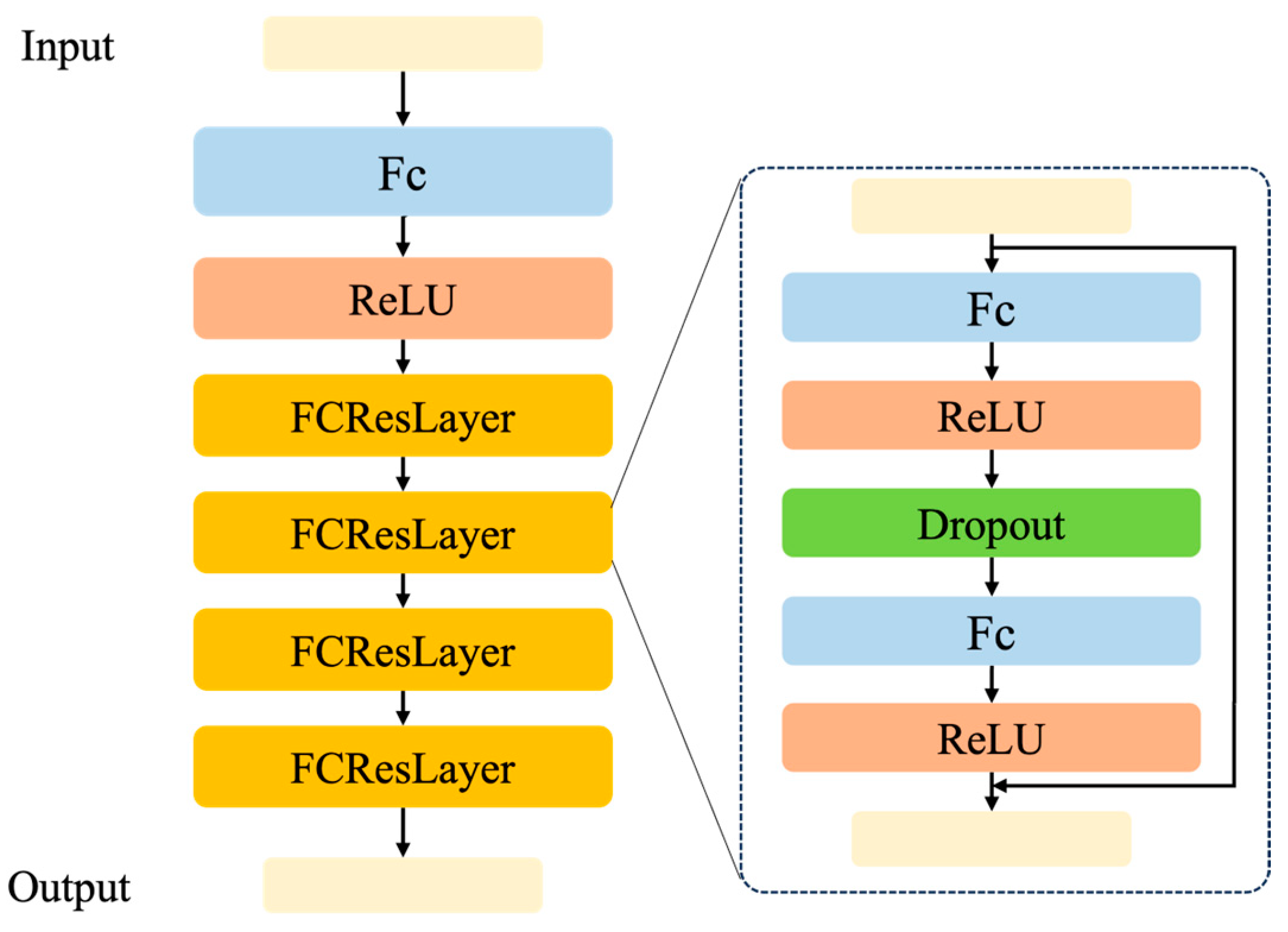
Inspired by Mac Aodha et al. [27], who proposed geographical priors for species recognition, we constructed a geographic feature extraction module (GFEM) for address location information. The structure of GFEM is shown in Figure 2. First, to provide a richer representation of geographic features, we started with a fully connected layer to transform the dimension of the location input S to a larger dimension. To acquire the nonlinear feature extraction capability, we used the ReLU activation function. Then, we stacked four FCResLayer blocks to enhance geographic feature representation. Every FCResLayer block contains two fully connected layers, two ReLU activation functions, a Dropout layer, and a skip connection. Finally, we obtained geographic features. Given the location input S, the geographic feature S_f was extracted by GFEM.

2.3. Image and Geographic Feature Fusion Module (IGFFM)

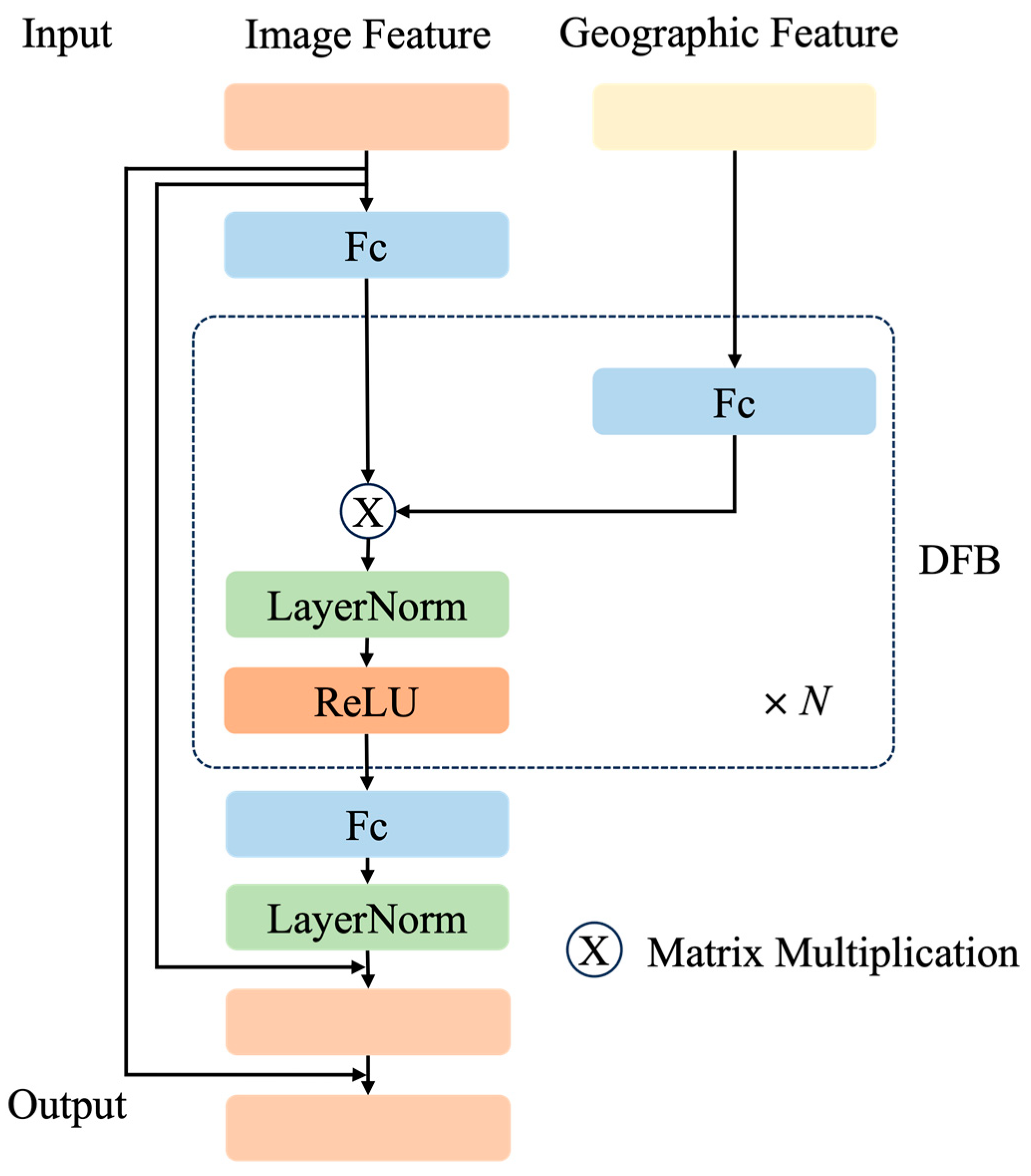
After acquiring image features or geographic features, inspired by Yang et al. [30], who proposed Dynamic MLP, we constructed an image and geographic feature fusion module (IGFFM) to fuse multimodal features. The structure of the IGFFM was shown in Figure 3.

Since the image feature dimension is larger than the geographic feature dimension, we decreased the image feature dimension to the same dimension as the geographic feature in order to reduce the memory cost. Then, we constructed a dynamic fusion block (DFB) to dynamically fuse image features and geographic features. In the DFB, one-dimensional geographic features were converted into the same shape as 3D image features, the depth interaction between image and geographic information was performed by matrix multiplication, and the enhanced image features were obtained after a LayerNorm layer and the ReLU activation function. Given the impact of geographic information on the recognition of different species, the number of stacked DFB modules is different for different species datasets. Finally, we extended the dimensions of the enhanced image features to be the same as the dimensions of the input image features and further enhanced them by a skip connection. To avoid forgetting the powerful image representation learning ability of CLIP, according to Equation (4), we used a residual connection to obtain the final image features by adding the enhanced image features with the original image features.

$$\widehat{I_f}=\alpha I_{ef}+\left(1-\alpha \right)I_f,$$

(4)

where $I_f$, $I_{ef}$, $\widehat{I_f}$, and $\alpha$ represent the original image features, enhanced image features, final image features, and the residual ratio, respectively

2.4. Species Prediction Probability Calculation

After acquiring fused image features, we multiplied the enhanced image features $\widehat{I_f}$ with the text features $T_f$ generated using the CLIP’s text encoder, and applied a Softmax function to calculate the predicted probability of the species, according to Equation (5).

$$p_i=Softmax\left(\widehat{I_f}{T}_f\right),$$

(5)

where $p_i$ denotes the prediction probabilities for the i-th species category, Softmax(·) represents the Softmax function.

3. Experiments

In this section, we present the dataset, experimental environment, implementation details, and evaluation metrics.

3.1. Datasets

The iNaturalist 2021 dataset [38] is a public species dataset containing 10,000 species in 11 supercategories. The dataset was collected and labeled by community scientists, and each image in the dataset contains latitude and longitude information at the time it was taken. We produced three few-shot datasets from the training and validation sets of this dataset by selecting three supercategories, namely Mammals, Reptiles, and Amphibians. Of these, Mammals contains 246 species, Reptiles contains 313 species, and Amphibians contains 170 species. Detailed descriptions of the three few-shot datasets are shown in

Table 1. Details of the training and validation set in the three few-shot datasets.

Species	Number of Species	Number of Images in the Training Set	Number of Images in the Testing Set
Mammals	246	3936	2460
Reptiles	313	5008	3130
Amphibians	170	2720	1700

.

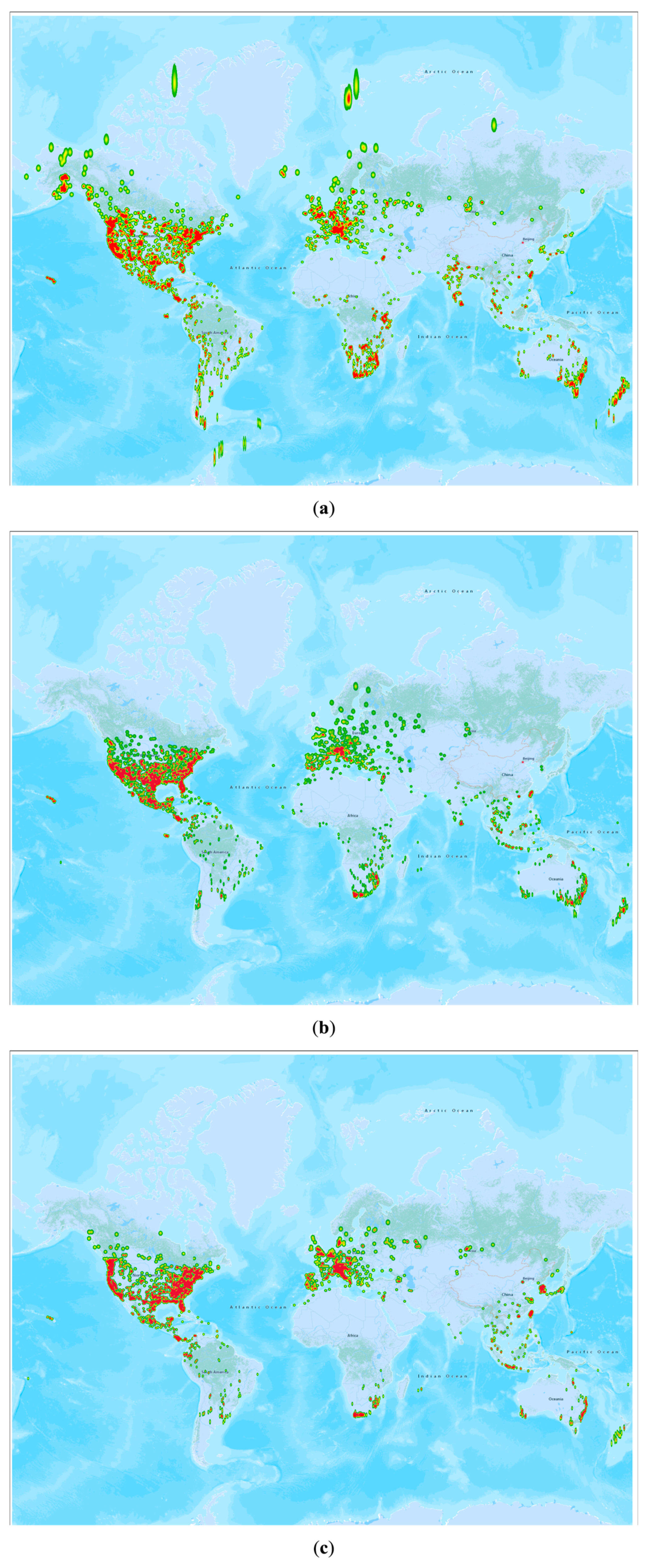
We combined all the geographic locations of the training and testing sets for each dataset and created heat maps of their corresponding geographic distributions for the three datasets. As can be seen in Figure 4, these species were distributed globally and occurred with different frequencies in different locations.

3.2. Experimental Setup, Implementation Details, and Evaluation Metrics

We implemented all the methods using PyTorch on an NVIDIA GeForce RTX 3090 (NVIDIA, Santa Clara, CA, USA). In our experiments, all input images were resized to 256 × 256 for training and testing. We trained our SG-CLIP using 1, 2, 4, 8, and 16 shots. During training, we used a Stochastic Gradient Descent (SGD) algorithm to optimize our proposed model, where the initial learning rate was set to 0.04, momentum was set to 0.9, and weight decay was set to 1 × 10⁻⁴. The CrossEntropyLoss function was used as the loss function, the batch size was set to 32, and the number of training epochs was set to 200. During testing, we used all the test images. We used Top-1 accuracy and Top-5 accuracy as evaluation metrics to validate our proposed method. For Tip-Adapter and Tip-Adapter-F, the same parameter settings were adopted, according to Zhang et al. [23].

4. Results

In this section, we compare our SG-CLIP with four baseline models, Zero-shot CLIP [20], Linear probe CLIP [20], Tip-Adapter [23], and Tip-Adapter-F [23]. Zero-shot CLIP, Tip-Adapter, Tip-Adapter-F, and SG-CLIP used the same textual prompt “A photo of a [class]”. Linear probe CLIP was adapted to the target dataset by training a linear classifier. To demonstrate the effectiveness and generalization of our proposed method, we conducted a number of comparison and ablation studies on different versions of CLIP.

4.1. Performance of Different Few-Shot Learning Methods on ViT-B/32

We chose the ViT-B/32 version of CLIP to compare the recognition performance of the different methods. The main results are displayed in

Table 2. Top-1 accuracy of few-shot species recognition by different methods under ViT-B/32. Data usage denotes the number of samples used for training.

Method	Data Usage	Mammals	Reptiles	Amphibians
Zero-shot CLIP	0	10.65%	3.93%	3.65%
Linear probe CLIP	1	13.94%	4.82%	4.77%
	2	16.55%	6.61%	7.29%
	4	22.85%	10.13%	9.35%
	8	31.26%	14.86%	14.65%
	16	38.70%	19.87%	18.41%
Tip-Adapter	1	16.14%	5.97%	5.53%
	2	18.66%	7.8%	6.82%
	4	21.75%	9.52%	8.24%
	8	26.75%	10.8%	10.82%
	16	30.24%	13.51%	13.71%
Tip-Adapter-F	1	18.29%	7.09%	6.24%
	2	22.89%	9.94%	9.35%
	4	26.59%	13.29%	12.57%
	8	34.02%	17.67%	15.88%
	16	41.26%	20.77%	20.53%
SG-CLIP	1	15.53%	8.85%	10.06%
	2	22.97%	12.36%	12.94%
	4	31.71%	19.20%	18.65%
	8	41.54%	27.53%	27.18%
	16	53.82%	37.38%	36.06%

. The results demonstrated in Table 2 show that SG-CLIP significantly outperforms all baseline methods in terms of recognition accuracy, proving that fusing geolocation information can improve the performance of few-shot species recognition.

Compared to Zero-shot CLIP, SG-CLIP achieved significant performance gains across all three species datasets. For the three species dataset, the performance of Zero-shot CLIP was exceeded by only the one-shot training setup. Under the 16-shot training setup, SG-CLIP boosts recognition accuracy by 5~10 times.

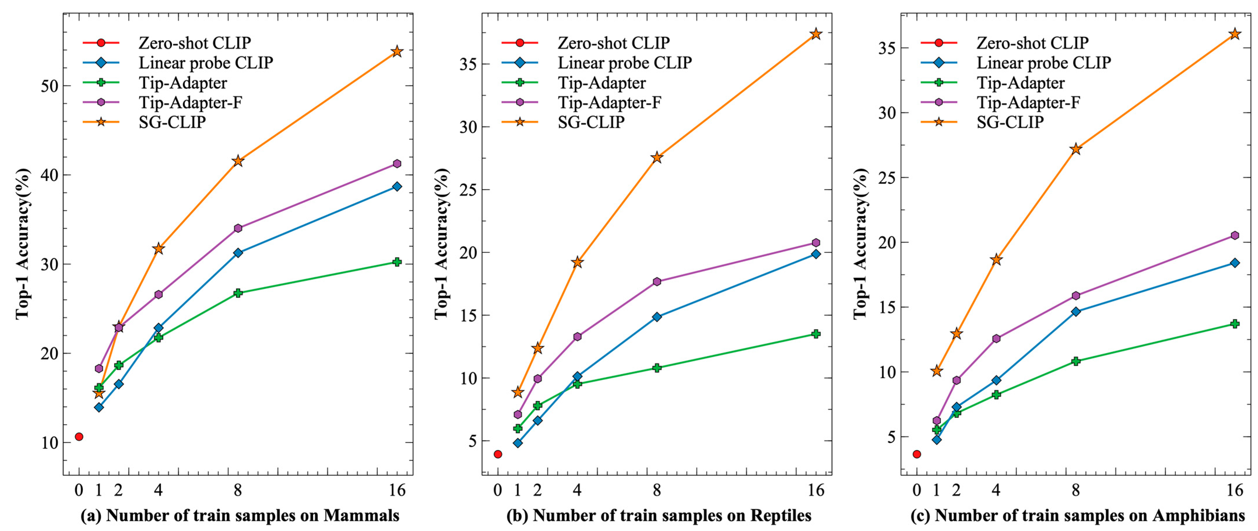
Compared to Linear probe CLIP, SG-CLIP achieved the best performance under all x-shot training settings, where x was 1, 2, 4, 8, and 16. As shown in Figure 4, as the number of training samples increases, the gap between SG-CLIP and Linear probe CLIP becomes more obvious. Under the 16-shot training setup, SG-CLIP improves the recognition accuracy by 15.12% (Mammals), 17.51% (Reptiles), and 17.65% (Amphibians).

Tip-Adapter and Tip-Adapter-F outperformed SG-CLIP only on the mammal dataset with the one-shot training setup. The SG-CLIP achieved significant performance gains on all three species datasets when the training samples are set to 2 or more. Compared to Tip-Adapter, the recognition accuracy of SG-CLIP was improved by 23.58% (Mammals), 23.87 (Reptiles), and 22.35% (Amphibians) with the 16-shot training setup. Similarly, the recognition accuracy of SG-CLIP was improved by 12.56% (Mammals), 17.39 (Reptiles), and 15.53% (Amphibians) compared to Tip-Adapter-F.

As shown in Figure 5, on the Mammals dataset, the recognition accuracy of Tip-Adapter-F was the highest, followed by Tip-Adapter, and SG-CLIP was only higher than Linear probe CLIP when the number of training samples was 1. As the number of training samples increased to more than 2, SG-CLIP gradually outperformed Tip Adapter and Tip Adapter. On the Reptiles and Amphibians datasets, SG-CLIP outperformed Tip-Adapter-F and Tip-Adapter at all settings of the number of training samples.

4.2. Performance of Few-Shot Species Recognition with Different Versions of CLIP

Further, we performed comparative experiments on different versions of CLIP, such as ViT-B/32 and ViT-L/14, to validate the generalizability of SG-CLIP. Compared with ViT-B/32, ViT-L/14 has more parameters and better feature extraction capability.

As can be seen from

Table 3. Performance of few-shot species recognition with different versions of CLIP. Data usage indicates the number of samples used for training. Bold indicates the best Top-1 recognition accuracy.

Image Encoder Version of CLIP	Dataset	Method	Data Usage
			0	1	2	4	8	16
ViT-B/32	Mammals	Zero-shot CLIP	10.65%	-	-	-	-	-
		Linear probe CLIP	-	13.94%	16.55%	22.85%	31.26%	38.70%
		Tip-Adapter	-	16.14%	18.66%	21.75%	26.75%	30.24%
		Tip-Adapter-F	-	18.29%	22.89%	26.59%	34.02%	41.26%
		SG-CLIP	-	15.53%	22.97%	31.71%	41.54%	53.82%
	Reptiles	Zero-shot CLIP	3.93%	-	-	-	-	-
		Linear probe CLIP	-	4.82%	6.61%	10.13%	14.86%	19.87%
		Tip-Adapter	-	5.97%	7.8%	9.52%	10.8%	13.51%
		Tip-Adapter-F	-	7.09%	9.94%	13.29%	17.67%	20.77%
		SG-CLIP	-	8.85%	12.36%	19.20%	27.54%	37.38%
	Amphibians	Zero-shot CLIP	3.65%	-	-	-	-	-
		Linear probe CLIP	-	4.77%	7.29%	9.35%	14.65%	18.41%
		Tip-Adapter	-	5.53%	6.82%	8.24%	10.82%	13.71%
		Tip-Adapter-F	-	6.24%	9.35%	12.57%	15.88%	20.53%
		SG-CLIP	-	10.06%	12.94%	18.65%	27.18%	36.06%
ViT-L/14	Mammals	Zero-shot CLIP	18.05%	-	-	-	-	-
		Linear probe CLIP	-	24.84%	31.67%	41.56%	50%	57.85%
		Tip-Adapter	-	28.9%	31.18%	36.5%	43.58%	48.5%
		Tip-Adapter-F	-	31.3%	38.17%	45.41%	52.48%	58.5%
		SG-CLIP	-	25.16%	36.18%	44.96%	55.61%	64.07%
	Reptiles	Zero-shot CLIP	5.37%	-	-	-	-	-
		Linear probe CLIP	-	9.2%	14.25%	20.38%	29.94%	35.46%
		Tip-Adapter	-	11.18%	13.48%	18.56%	21.95%	26.29%
		Tip-Adapter-F	-	13.23%	18.53%	25.97%	30.45%	37.22%
		SG-CLIP	-	14.72%	21.02%	30.03%	39.81%	49.23%
	Amphibians	Zero-shot CLIP	4.71%	-	-	-	-	-
		Linear probe CLIP	-	6.82%	9.53%	16.06%	21.35%	27%
		Tip-Adapter	-	8.94%	9.88%	11.53%	15.24%	18.53%
		Tip-Adapter-F	-	8.29%	13.53%	16.59%	23.41%	28.18%
		SG-CLIP	-	13.24%	18.24%	24.65%	33.18%	43.82%

, the recognition accuracies of Zero-shot CLIP, Linear probe CLIP, Tip-Adapter, Tip-Adapter-F, and SG-CLIP were significantly improved as the model became larger. Under the 16-shot training setup on the Mammals dataset, the recognition accuracy of SG-CLIP under ViT-L/14 improved from 53.82% to 64.07% compared to SG-CLIP under ViT-B/32, which gained a 10.25% improvement. Similarly, improvements of 11.85% and 7.22% were obtained on the Reptiles and Amphibians datasets, respectively.

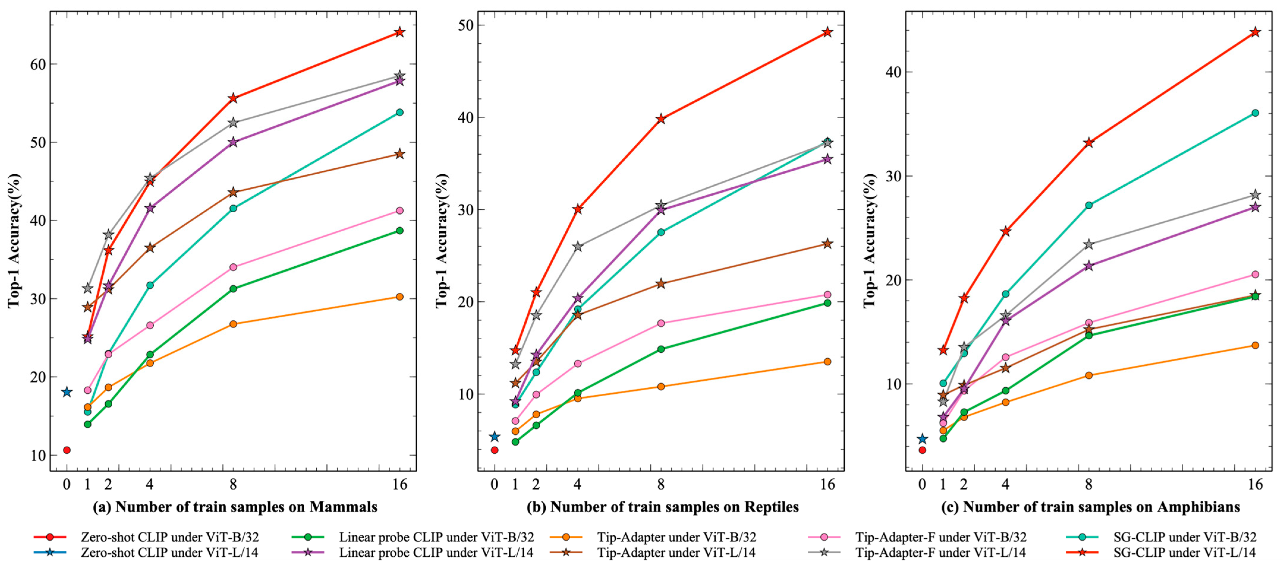
From Figure 6, it can be observed that SG-CLIP achieved the highest level of recognition accuracy when the number of training samples for each category was set to 16. Tip-Adapter-F and Linear probe CLIP followed after SG-CLIP, and their performance improved as the number of training samples increased. Finally, Tip-Adapter had the lowest recognition accuracy among all the few-shot recognition methods. On the Reptiles and Amphibians datasets, SG-CLIP achieved the best performance and substantially outperformed other methods in all training sample setups. The gap became more pronounced as the number of training samples in each class increased. On the Mammals dataset, SG-CLIP did not have the highest recognition accuracy when the training sample setting was less than 4; SG-CLIP only outperformed the other methods when it exceeded 4.

4.3. Time Efficiency Analysis

To evaluate our proposed method more comprehensively, we conducted time efficiency analysis experiments, the results of which are shown in

Table 4. Comparative experiments on the training time of different methods. The image encoder of CLIP is ViT-L/14. The training time was tested on a NVIDIA GeForce RTX 3090 GPU.

Method	Training Time
	Mammals	Reptiles	Amphibians
Zero-shot CLIP	0	0	0
Linear probe CLIP	51.64 s	43.79 s	16.57 s
Tip-Adapter	0	0	0
Tip-Adapter-F	6.57 m	8.20 m	4.7 m
SG-CLIP	3.31 h	4.49 h	2.12 h

. The training time for SG-CLIP was far superior to that of other methods. Linear probe CLIP freezes the CLIP to extract features and adds a linear layer for classification, requiring very little training time. Tip-Adapter improves the species recognition performance by fusing the predictions of the pre-constructed key-value cache model with the predictions of Zero-shot CLIP, which is a training-free adaptation method, and thus it and Zero-shot CLIP have no additional training cost. Tip-Adapter-F further fine-tunes the keys of the cached models in Tip-Adapter as learnable parameters, thus introducing additional training time, usually within only a few minutes. SG-CLIP introduces two modules, GFEM and IGFFM, for feature extraction of geolocation information and deep fusion between images and geographic features, respectively, so it requires a lot of training time.

4.4. Ablation Studies

We conducted three ablation studies for SG-CLIP on the residual ratio α, the number of DFBs in IGFFM, and geographic information.

We first performed an ablation study by varying the residual ratio α. From

Table 5. Ablation study on different residual ratios. The CLIP version is ViT-B/32. The number of DFBs in IGFEM is 2. The recognition accuracy in the table is Top-1 accuracy.

Residual Ratio α	Mammals	Reptiles	Amphibians
0.2	49.07%	34.09%	30.47%
0.4	51.67%	36.23%	32.47%
0.6	52.07%	33.76%	33.46%
0.8	53.82%	37.12%	33.71%
1.0	52.64%	37.03%	33.76%

, we can see that the residual ratios were different on different datasets, where the best residual ratio on Mammals was 0.8, the best residual ratio on Reptiles was 0.8, and the best residual ratio on Amphibians was 1.0. In general, fusing image and geographic features and then adding them to the original image features better improves the performance of few-shot species recognition.

Moreover, we performed an ablation study by adjusting the number of DFBs in IGFFM. As shown in

Table 6. Ablation study on different numbers of DFB in IGFEM. The CLIP version is ViT-B/32. The residual ratios on Mammals, Reptiles, and Amphibians are 0.8, 0.8, and 1.0, respectively. The recognition accuracy in the table is Top-1 accuracy.

Number	Mammals	Reptiles	Amphibians
1	50.94%	34.22%	33.59%
2	53.82%	37.12%	33.76%
3	52.36%	37.38%	33.65%
4	52.73%	36.68%	36.06%
5	51.46%	36.52%	35%

, we observed that the number of DFBs in IGFFM is different on different datasets. Specifically, the number of DFBs in IGFFM was 2 on Mammals, 3 on Reptiles, and 4 on Amphibians. We observed that the less common the species in the CLIP training set, the more DFBs in IGFFM were required.

Finally, we conducted an ablation study on geographic information. As can be seen from

Table 7. Ablation study of geographic information. The CLIP version is ViT-L/14. The residual ratios on Mammals, Reptiles, and Amphibians are 0.8, 0.8, and 1.0, respectively. The number of DFBs in IGFFM on Mammals, Reptiles and Amphibians are 2, 3, and 4, respectively. The recognition accuracy in the table is Top-1 accuracy. The number of samples is 16-shot.

Number	Mammals	Reptiles	Amphibians
w/longitude	57.76%	41.21%	33.82%
w/latitude	55.89%	36.58%	27.76%
w/(latitude, longitude)	64.07%	49.23%	43.82%

, fusing either longitude or latitude helps to improve the species recognition performance under the 16-shot training setup. Further, the recognition performance on all three species datasets when fusing longitude or latitude alone is lower than when fusing both longitude and latitude.

4.5. Visualization Analysis

SG-CLIP has been shown to improve few-shot species recognition accuracy across species datasets. To better understand the mechanism of how SG-CLIP works, we selected the top 15 species from the Mammals dataset and used t-SNE [39] to visualize the image representations extracted by different methods as a point. As shown in Figure 7, from ViT-B/32 to ViT-B/14, the cluster results of Zero-shot CLIP and SG-CLIP improved. SG-CLIP generated more discriminative image representations compared to Zero-shot CLIP under ViT-B/32 and ViT-L/14. This was due to the fact that SG-CLIP utilizes geolocation information for multiple interactions with image features in higher dimensions.

4.6. Case Studies

To demonstrate the effectiveness of the proposed method in practical application, we executed a case study on a subset of Mammals. First, we created Mammals-20 by selecting the top 20 species from the Mammals dataset. Then, we performed comparative experiments of different methods on Mammals-20 under ViT-L/14. From

Table 8. Performance of few-shot species recognition by different methods under ViT-L/14. Data usage denotes the number of samples used for training.

Method	Data Usage	Accuracy
		Top-1	Top-5
Zero-shot CLIP	0	37%	63%
Tip-Adapter	1	46%	71%
	2	54.5%	78.5%
	4	62.5%	87%
	8	67%	93%
	16	74%	95.5%
Tip-Adapter-F	1	44.5%	76%
	2	52.5%	77%
	4	67.5%	92%
	8	72.5%	96.5%
	16	75.5%	97.5%
SG-CLIP	1	52.5%	85%
	2	60%	88.5%
	4	72%	92%
	8	80.5%	96%
	16	89%	97.5%

, it can be seen that the Top-1 and Top-5 recognition accuracies of SG-CLIP were much better than the other methods under all training sample setups (1, 2, 4, 8, and 16). Specifically, SG-CLIP achieved the best Top-1 and Top-5 accuracies of 89% and 97.5%, respectively, for the 16-shot training setup. Although the Top-5 accuracy of Tip-Adapter-F was the same as the recognition accuracy of SG-CLIP, the Top-1 accuracy of 75.5% was much lower than that of SG-CLIP. Compared to the 37% Top-1 recognition accuracy of the Zero-shot CLIP on Mammals-20, the SG-CLIP with the 16-shot training setup is sufficient for real-world precision recognition applications.

5. Discussion

In this work, we explored for the first time the potential of using geographic information in foundation model-based species classification tasks, and demonstrated that fusing geolocation information from species observations can help improve performance in few-shot species recognition.

Additional information, like geographic location information and time information, can benefit species recognition. Many studies [27,30,40,41] have utilized geographic information to improve the performance of species recognition. However, the above studies on species recognition are mainly built on traditional ResNet and ViT-based visual models, while our proposed method is built on foundation models such as CLIP. In addition, the amount of data used for training is another difference; our approach requires a relatively small number of training samples.

There are many studies exploring the potential of CLIP as an emerging paradigm for zero-shot or few-shot species recognition. CLIP-Adapter [21] constructs a new bottleneck layer to fine-tune the image or text features extracted by the pretrained CLIP to the new species dataset. Tip-Adapter [23] utilizes the training set from the new species dataset to construct a key-value caching model and improve the performance of the CLIP for species recognition through feature retrieval. Maniparambil et al. [36] used GPT-4 to generate species descriptions in combination with an adapter constructed by the self-attention mechanism to improve performance in zero-shot and few-shot species recognition. The above work is either improved in the image branch of CLIP or in the text branch of CLIP. Unlike the above work, we added a geographic information branch to improve species recognition performance with the help of a priori knowledge of geographic location.

First, we validated our proposed method on three species supercategories (Mammals, Reptiles, and Amphibians), demonstrating that fusing geographic information facilitates species recognition and was effective across categories. Then, we performed experiments on different versions of CLIP (ViT-B/32 and ViT-L/14), and it can be found that as the feature extraction capability of the pretrained CLIP model is enhanced, the performance of our method is enhanced accordingly. This provides strong confidence for building foundation models for taxonomic classification in the future. Next, we performed rigorous ablation experiments that demonstrate the importance of our different modules and also show that appropriate hyperparameters need to be set for different species’ supercategories. These hyperparameters are usually positively correlated with the ease of species recognition. Finally, from the visualization results in Figure 7, it can be noticed that different species become easier to distinguish after incorporating geolocation information.

However, our work faces two limitations. First, the data used to train the CLIP model came from the Internet, where there is relatively little data on species, leading to poor performance of CLIP on the species classification task. Second, due to the difficulty of species recognition, the residual ratio and the number of DFB are variable on different species datasets, requiring a manual search for appropriate values.

In the future, we will consider allowing the proposed model to automatically learn appropriate parameters such as the residual rate and the number of DFBs. In addition, we will validate the proposed method on other foundation models.

6. Conclusions

In this paper, we proposed SG-CLIP, a few-shot species-recognition method of CLIP that leverages geographic information about species. To the best of our knowledge, we are the first to integrate geographic information for CLIP-driven few-shot species recognition. First, to harness the powerful image representation learning capabilities of foundation models such as CLIP, we used a pretrained CLIP model to extract species’ image features and corresponding textual features. Then, to better utilize geographic information, we constructed a geographic feature extraction module to transform structured geographic information into geographic features. Next, to fully exploit the potential of geographic features, we constructed a multimodal fusion module to enable deep interaction between image features and geographic features to obtain enhanced image features. Finally, we computed the similarity between the enhanced image features and the text features to obtain the predictions of the species. Through extensive experiments on different species datasets, it can be observed that utilizing geolocation information can effectively improve the performance of CLIP for species recognition, and significantly outperform other advanced methods.

For species recognition scenarios under data constraints, such as rare and endangered wildlife recognition, our model can be used as the first step for accurate recognition to improve the level of automated species recognition, accelerate species data annotation, and provide preliminary data support work for the subsequent design and iteration of models dedicated to the recognition of specific species. We hope that our model can help build better species distribution models for biodiversity research. In future work, we will focus on the impact of geographic information on species recognition at different regional scales.

References

1. Hong, P.; Schmid, B.; De Laender, F.; Eisenhauer, N.; Zhang, X.; Chen, H.; Craven, D.; De Boeck, H.J.; Hautier, Y.; Petchey, O.L.; et al. Biodiversity Promotes Ecosystem Functioning despite Environmental Change. Ecol. Lett. 2022, 25, 555–569. [Google Scholar] [CrossRef] [PubMed]
2. Simkin, R.D.; Seto, K.C.; McDonald, R.I.; Jetz, W. Biodiversity Impacts and Conservation Implications of Urban Land Expansion Projected to 2050. Proc. Natl. Acad. Sci. USA 2022, 119, e2117297119. [Google Scholar] [CrossRef] [PubMed]
3. Gaston, K.J.; O’Neill, M.A. Automated Species Identification: Why Not? Philos. Trans. R. Soc. B Biol. Sci. 2004, 359, 655–667. [Google Scholar] [CrossRef] [PubMed]
4. Bojamma, A.M.; Shastry, C. A Study on the Machine Learning Techniques for Automated Plant Species Identification: Current Trends and Challenges. Int. J. Inf. Tecnol. 2021, 13, 989–995. [Google Scholar] [CrossRef]
5. Tuia, D.; Kellenberger, B.; Beery, S.; Costelloe, B.R.; Zuffi, S.; Risse, B.; Mathis, A.; Mathis, M.W.; van Langevelde, F.; Burghardt, T.; et al. Perspectives in Machine Learning for Wildlife Conservation. Nat. Commun. 2022, 13, 792. [Google Scholar] [CrossRef] [PubMed]
6. Chen, R.; Little, R.; Mihaylova, L.; Delahay, R.; Cox, R. Wildlife Surveillance Using Deep Learning Methods. Ecol. Evol. 2019, 9, 9453–9466. [Google Scholar] [CrossRef]
7. Duggan, M.T.; Groleau, M.F.; Shealy, E.P.; Self, L.S.; Utter, T.E.; Waller, M.M.; Hall, B.C.; Stone, C.G.; Anderson, L.L.; Mousseau, T.A. An Approach to Rapid Processing of Camera Trap Images with Minimal Human Input. Ecol. Evol. 2021, 11, 12051–12063. [Google Scholar] [CrossRef]
8. Gomez Villa, A.; Salazar, A.; Vargas, F. Towards Automatic Wild Animal Monitoring: Identification of Animal Species in Camera-Trap Images Using Very Deep Convolutional Neural Networks. Ecol. Inform. 2017, 41, 24–32. [Google Scholar] [CrossRef]
9. Xie, Y.; Jiang, J.; Bao, H.; Zhai, P.; Zhao, Y.; Zhou, X.; Jiang, G. Recognition of Big Mammal Species in Airborne Thermal Imaging Based on YOLO V5 Algorithm. Integr. Zool. 2023, 18, 333–352. [Google Scholar] [CrossRef]
10. Huang, S.; Xu, Z.; Tao, D.; Zhang, Y. Part-Stacked CNN for Fine-Grained Visual Categorization. In Proceedings of the 2016 IEEE Conference on Computer Vision and Pattern Recognition (CVPR), Las Vegas, NV, USA, 27–30 June 2016; IEEE: Piscataway, NJ, USA; pp. 1173–1182. [Google Scholar]
11. Lv, X.; Xia, H.; Li, N.; Li, X.; Lan, R. MFVT: Multilevel Feature Fusion Vision Transformer and RAMix Data Augmentation for Fine-Grained Visual Categorization. Electronics 2022, 11, 3552. [Google Scholar] [CrossRef]
12. Li, M.; Zhou, G.; Cai, W.; Li, J.; Li, M.; He, M.; Hu, Y.; Li, L. Multi-Scale Sparse Network with Cross-Attention Mechanism for Image-Based Butterflies Fine-Grained Classification. Appl. Soft Comput. 2022, 117, 108419. [Google Scholar] [CrossRef]
13. He, J.; Kortylewski, A.; Yuille, A. CORL: Compositional Representation Learning for Few-Shot Classification. In Proceedings of the IEEE/CVF Winter Conference on Applications of Computer Vision, Waikoloa, HI, USA, 2–7 January 2023; pp. 3890–3899. [Google Scholar]
14. Zhang, Q.; Yi, X.; Guo, J.; Tang, Y.; Feng, T.; Liu, R. A Few-Shot Rare Wildlife Image Classification Method Based on Style Migration Data Augmentation. Ecol. Informatics 2023, 77, 102237. [Google Scholar] [CrossRef]
15. Snell, J.; Swersky, K.; Zemel, R. Prototypical Networks for Few-Shot Learning. In Advances in Neural Information Processing Systems; Curran Associates, Inc.: Long Beach, CA, USA, 2017; Volume 30. [Google Scholar]
16. Guo, Z.; Zhang, L.; Jiang, Y.; Niu, W.; Gu, Z.; Zheng, H.; Wang, G.; Zheng, B. Few-Shot Fish Image Generation and Classification. In Proceedings of the Global Oceans 2020: Singapore—U.S. Gulf Coast, Biloxi, MS, USA, 5–14 October 2020; pp. 1–6. [Google Scholar]
17. Zhai, J.; Han, L.; Xiao, Y.; Yan, M.; Wang, Y.; Wang, X. Few-Shot Fine-Grained Fish Species Classification via Sandwich Attention CovaMNet. Front. Mar. Sci. 2023, 10, 1149186. [Google Scholar] [CrossRef]
18. Lu, J.; Zhang, S.; Zhao, S.; Li, D.; Zhao, R. A Metric-Based Few-Shot Learning Method for Fish Species Identification with Limited Samples. Animals 2024, 14, 755. [Google Scholar] [CrossRef]
19. Xu, S.-L.; Zhang, F.; Wei, X.-S.; Wang, J. Dual Attention Networks for Few-Shot Fine-Grained Recognition. In Proceedings of the AAAI Conference on Artificial Intelligence, Palo Alto, CA, USA, 22 February–1 March 2022; pp. 2911–2919. [Google Scholar] [CrossRef]
20. Radford, A.; Kim, J.W.; Hallacy, C.; Ramesh, A.; Goh, G.; Agarwal, S.; Sastry, G.; Askell, A.; Mishkin, P.; Clark, J.; et al. Learning Transferable Visual Models From Natural Language Supervision. In Proceedings of the 38th International Conference on Machine Learning, PMLR, Virtual, 18–24 July 2021; pp. 8748–8763. [Google Scholar]
21. Gao, P.; Geng, S.; Zhang, R.; Ma, T.; Fang, R.; Zhang, Y.; Li, H.; Qiao, Y. CLIP-Adapter: Better Vision-Language Models with Feature Adapters. Int. J. Comput. Vis. 2023, 132, 581–595. [Google Scholar] [CrossRef]
22. Zhou, K.; Yang, J.; Loy, C.C.; Liu, Z. Learning to Prompt for Vision-Language Models. Int. J. Comput. Vis. 2022, 130, 2337–2348. [Google Scholar] [CrossRef]
23. Zhang, R.; Zhang, W.; Fang, R.; Gao, P.; Li, K.; Dai, J.; Qiao, Y.; Li, H. Tip-Adapter: Training-Free Adaption of CLIP for Few-Shot Classification. In Computer Vision—ECCV 2022; Avidan, S., Brostow, G., Cissé, M., Farinella, G.M., Hassner, T., Eds.; Springer: Cham, Switzerland, 2022; pp. 493–510. [Google Scholar]
24. Guo, Z.; Zhang, R.; Qiu, L.; Ma, X.; Miao, X.; He, X.; Cui, B. CALIP: Zero-Shot Enhancement of CLIP with Parameter-Free Attention. In Proceedings of the AAAI Conference on Artificial Intelligence, Washington, DC, USA, 7–14 February 2023; pp. 746–754. [Google Scholar] [CrossRef]
25. Parashar, S.; Lin, Z.; Li, Y.; Kong, S. Prompting Scientific Names for Zero-Shot Species Recognition. In Proceedings of the 2023 Conference on Empirical Methods in Natural Language Processing, Singapore, 6–10 December 2023; pp. 9856–9861. [Google Scholar]
26. Menon, S.; Vondrick, C. Visual Classification via Description from Large Language Models. In Proceedings of the Eleventh International Conference on Learning Representations, Kigali, Rwanda, 29 September 2022. [Google Scholar]
27. Mac Aodha, O.; Cole, E.; Perona, P. Presence-Only Geographical Priors for Fine-Grained Image Classification. In Proceedings of the IEEE/CVF International Conference on Computer Vision, Seoul, Republic of Korea, 27 October 2019; pp. 9596–9606. [Google Scholar]
28. Terry, J.C.D.; Roy, H.E.; August, T.A. Thinking like a Naturalist: Enhancing Computer Vision of Citizen Science Images by Harnessing Contextual Data. Methods Ecol. Evol. 2020, 11, 303–315. [Google Scholar] [CrossRef]
29. de Lutio, R.; She, Y.; D’Aronco, S.; Russo, S.; Brun, P.; Wegner, J.D.; Schindler, K. Digital Taxonomist: Identifying Plant Species in Community Scientists’ Photographs. ISPRS J. Photogramm. Remote Sens. 2021, 182, 112–121. [Google Scholar] [CrossRef]
30. Yang, L.; Li, X.; Song, R.; Zhao, B.; Tao, J.; Zhou, S.; Liang, J.; Yang, J. Dynamic MLP for Fine-Grained Image Classification by Leveraging Geographical and Temporal Information. In Proceedings of the 2022 IEEE/CVF Conference on Computer Vision and Pattern Recognition (CVPR), New Orleans, LA, USA, 18 June 2022; IEEE: Piscataway, NJ, USA; pp. 10935–10944. [Google Scholar]
31. Liu, L.; Han, B.; Chen, F.; Mou, C.; Xu, F. Utilizing Geographical Distribution Statistical Data to Improve Zero-Shot Species Recognition. Animals 2024, 14, 1716. [Google Scholar] [CrossRef]
32. He, K.; Zhang, X.; Ren, S.; Sun, J. Deep Residual Learning for Image Recognition. In Proceedings of the IEEE Conference on Computer Vision and Pattern Recognition, Las Vegas, NV, USA, 27 June 2016; pp. 770–778. [Google Scholar]
33. Dosovitskiy, A.; Beyer, L.; Kolesnikov, A.; Weissenborn, D.; Zhai, X.; Unterthiner, T.; Dehghani, M.; Minderer, M.; Heigold, G.; Gelly, S.; et al. An Image Is Worth 16 × 16 Words: Transformers for Image Recognition at Scale. Available online: https://arxiv.org/abs/2010.11929v2 (accessed on 26 January 2024).
34. Vaswani, A.; Shazeer, N.; Parmar, N.; Uszkoreit, J.; Jones, L.; Gomez, A.N.; Kaiser, Ł.; Polosukhin, I. Attention Is All You Need. In Advances in Neural Information Processing Systems; Curran Associates, Inc.: Red Hook, NY, USA, 2017; pp. 6000–6010. [Google Scholar]
35. Zhang, R.; Guo, Z.; Zhang, W.; Li, K.; Miao, X.; Cui, B.; Qiao, Y.; Gao, P.; Li, H. PointCLIP: Point Cloud Understanding by CLIP. In Proceedings of the IEEE/CVF Conference on Computer Vision and Pattern Recognition, New Orleans, LA, USA, 18–24 June 2022; pp. 8552–8562. [Google Scholar]
36. Maniparambil, M.; Vorster, C.; Molloy, D.; Murphy, N.; McGuinness, K.; O’Connor, N.E. Enhancing CLIP with GPT-4: Harnessing Visual Descriptions as Prompts. In Proceedings of the IEEE/CVF International Conference on Computer Vision, Paris, France, 2–6 October 2023; pp. 262–271. [Google Scholar]
37. Deng, H.; Zhang, Z.; Bao, J.; Li, X. AnoVL: Adapting Vision-Language Models for Unified Zero-Shot Anomaly Localization. arXiv 2023, arXiv:2308.15939. [Google Scholar]
38. Van Horn, G. Oisin Mac Aodha. iNat Challenge 2021-FGVC8. Available online: https://kaggle.com/competitions/inaturalist-2021 (accessed on 18 January 2024).
39. Van der Maaten, L.; Hinton, G. Visualizing Data Using T-SNE. J. Mach. Learn. Res. 2008, 9, 2579–2605. [Google Scholar]
40. Chu, G.; Potetz, B.; Wang, W.; Howard, A.; Song, Y.; Brucher, F.; Leung, T.; Adam, H. Geo-Aware Networks for Fine-Grained Recognition. In Proceedings of the 2019 IEEE/CVF International Conference on Computer Vision Workshop (ICCVW), Seoul, Republic of Korea, 27 October 2019; pp. 247–254. [Google Scholar]
41. Tang, K.; Paluri, M.; Fei-Fei, L.; Fergus, R.; Bourdev, L. Improving Image Classification with Location Context. In Proceedings of the 2015 IEEE International Conference on Computer Vision (ICCV), Santiago, Chile, 7 December 2015; pp. 1008–1016. [Google Scholar]
Figure 1. The overall framework of SG-CLIP for few-shot species recognition. It contains three paths for text, image, and geographic information, respectively. The geographic feature is obtained by GFEM. The parameters of GFEM and IGFFM are learnable.
Remotesensing 16 02238 g001
Figure 2. The structure of GFEM for geographic feature extraction. The dashed box is the structure of the FCResLayer.
Remotesensing 16 02238 g002
Figure 3. The structure of IGFFM for image and geographic feature fusion, where Fc denotes the fully connected layer, ReLU denotes the ReLU activation function, and LayerNorm denotes layer normalization. DFB denotes the dynamic fusion block. DFB is used recursively, where N is the number of DFB modules.
Remotesensing 16 02238 g003
Figure 4. Heatmaps of the geolocation distribution. (a) Mammals. (b) Reptiles. (c) Amphibians. Different colors indicate the number of species at different locations. Green indicates relatively little data and red indicates a large number.
Remotesensing 16 02238 g004
Figure 5. Performance comparison of different methods with different training samples on different datasets. (a) Mammals. (b) Reptiles. (c) Amphibians.
Remotesensing 16 02238 g005
Figure 6. Comparison of few-shot species recognition accuracy on different datasets under different versions of CLIP. (a) Mammals. (b) Reptiles. (c) Amphibians.
Remotesensing 16 02238 g006
Figure 7. Visualization of t-SNE representations under different methods. (a) Zero-shot CLIP under ViT-B/32. (b) Zero-shot CLIP under ViT-L/14. (c) SG-CLIP under ViT-B/32. (d) SG-CLIP under ViT-L/14.
Remotesensing 16 02238 g007