Adaptive Multi-Hypothesis Marginal Bayes Filter for Tracking Multiple Targets

Abstract

Tracking multiple targets in the presence of unknown number of targets, missed detection, clutter, and noise is a challenging problem. To cope with this problem, a novel approach for generating the potential birth targets was developed, a mathematical model for multiple hypotheses was established, and an adaptive multi-hypothesis marginal Bayes filter is herein proposed in terms of the established mathematical model for multiple hypotheses and the novel birth approach. This filter delivers the existence probabilities of targets and their probability density functions. It uses multiple hypotheses to solve the data association problem to form the existence probabilities of targets and their probability density functions. To obviate the requirement for prior birth models, this filter uses the observations from two consecutive time steps to establish the birth models adaptively. Its tracking performance was tested by comparing it with other adaptive filters, showing that the proposed filter is robust, and it can obtain higher tracking accuracy than other filters.

1. Introduction

Multi-target tracking (MTT) is a process that uses the sensor observations with clutter, missed detection, and noise to acquire the state vectors of targets at different time steps [1,2,3]. It finds numerous applications in maritime surveillance, air traffic monitoring, self-driving vehicles, and advanced driver-assistance systems [4], thereby attracting the extensive attention of scholars [5,6,7,8,9]. Many approaches such as random finite set (RFS) [1,2], multiple hypothesis tracking [10], and joint probabilistic data association [11] have been proposed to perform multi-target tracking.

The conventional RFS methods for MTT only concern multi-object filtering [1,2]. Their objective is to estimate the object states at different time steps. These methods do not attempt to generate object trajectories. The typical representatives of the conventional RFS methods are the multi-Bernoulli filter [12] and probability hypothesis density filter [13,14]. These two filters have also been extended by several scholars to track maneuvering targets [15] and extended targets [16,17,18,19].

To break through the restriction of RFS on providing target trajectories, Vo et al. proposed the labeled RFS [20,21]. Unlike the RFS approach that only provides the states of objects, the labeled RFS approach can provide both the states of objects and their trajectories. Moreover, the high signal to noise ratio that is required in the RFS approach is also obviated in the labeled RFS approach. The labeled RFS approach can give higher tracking accuracy at a larger computational cost than the RFS approach. This is because the former uses multiple hypotheses, and the number of hypotheses may increase exponentially as the recursion increases. To decrease the computational cost of the labeled RFS approach, Vo et al. proposed an efficient implementation of the generalized labeled multi-Bernoulli (GLMB) filter [22]. Based on the labeled RFS, the tracking filters for spawning objects [23], weak objects [24], maneuvering objects [25], and extended objects [26] have also been proposed by several scholars.

The choice or establishment of birth models in the RFS filters and labeled RFS filters is a challenging problem. The conventional RFS filters [12,13,14] and labeled RFS filters [20,21,22] assume that targets appear from fixed locations such as airports, wharves, or doors. This assumption disenables these filters to track the objects appearing from unknown locations. Several adaptive filters based on the RFS and labeled RFS have been proposed to break through this limitation. Instead of using the prior locations, the adaptive filters in [27,28,29,30] use the observations at each time step to form the birth models. The drawback of these filters is that they assume that the covariance matrix of each birth object is fixed and known. To overcome this drawback, the adaptive filters in [31,32,33] use the measurements from two consecutive time steps to establish the birth models, and the adaptive GLMB (AGLMB) filter in [34] uses the measurements from three consecutive time steps to generate the birth tracks. The main weakness of the AGLMB filter is that some of the newborn tracks may be false tracks. To decrease the false-track probability, combining the logic-based track initiation technique into the marginal multi-target Bayesian (MTB) filter, Liu et al. proposed the adaptive MTB filter with assignment of measurements (AAMMTB filter) [35]. Compared with the AGLMB filter [34], the AAMMTB filter achieves high tracking accuracy at a low computational cost [35]. The AGLMB filter and AAMMTB filter use the observations of three time steps to generate the birth tracks. Each birth track is regarded as a real track in these two adaptive filters. The difference between them is that the AGLMB filter uses the rule-based track initiation technique, while the AAMMTB filter uses the logic-based track initiation technique. The experimental results have shown that the AAMMTB filter has better performance than the AGLMB filter and other adaptive filters [35].

To track multiple targets more efficiently in the presence of unknown number of targets, missed detection, clutter, and noise, an adaptive multi-hypothesis marginal Bayes (AMHMB) filter is proposed in this article. Instead of delivering multiple hypotheses in the filtering recursion, the AMHMB filter propagates the probability density function (PDF) of each potential object and its existence probability. It uses the multiple hypotheses to solve the data association problem to form the PDFs of potential objects and their existence probabilities and employs the measurements from two time steps to generate the potential birth objects. Compared with the birth approach in [29,30], the birth approach in this article can form the covariance matrix of the potential birth target adaptively, thereby obviating the need for a prior covariance matrix. Unlike the AGLMB filter and AAMMTB filter that use the measurements from three time steps to generate the birth tracks, the AMHMB filter uses the measurements from two time steps to establish the potential birth targets. The simulation results exhibit that the AMHMB filter is robust, and it can obtain higher tracking accuracy than other filters.

The contributions of this article are as follows:

A novel approach for generating the potential birth targets is developed. In this approach, the initial state and error covariance of the potential birth target is formed adaptively, and its existence probability is given in terms of the unused probabilities of the two observations for generating this potential birth target;

A mathematical model for multiple hypotheses is established to solve the data association problem in the MTT. The multiple hypotheses are used for forming the PDFs of potential objects and their existence probabilities;

Based on the mathematical model for multiple hypotheses and the novel birth approach, an AMHMB filter is proposed.

The rest of the paper is as follows: The object dynamic model, the sensor observation model and the generating method for potential birth targets are provided in Section 2, and then, the mathematical model for multiple hypotheses is given in Section 3. In Section 4, the AMHMB filter is presented. Simulation results are given in Section 5 to compare the AMHMB filter with other filters. Conclusions are summarized in Section 6.

2. Generation of Potential Birth Targets

In this article, the object dynamic and sensor observation models are as follows:

$${\mathit{x}}_k={\mathit{\Phi }}_{k-1}{\mathit{x}}_{k-1}+w_{k-1}$$

(1)

$${\mathit{z}}_k=h({\mathit{x}}_k)+v_k$$

(2)

where ${\mathit{x}}_k$ and ${\mathit{z}}_k$ denote the state of an object and its observation; ${\mathit{\Phi }}_{k-1}$ and $h(·)$ are the state transition matrix and nonlinear measurement function; $w_{k-1}$ is process noise; and $v_k$ is observation noise. These two noises are the zero-mean Gaussian noises. The covariance of the former is ${\mathit{Q}}_{k-1}$, and the covariance of the latter is ${\mathit{R}}_k$.

In the surveillance region, a radar at position ${\left[\begin{array}{cc}{x}_s& y_s\end{array}\right]}^{\mathrm{T}}$ observes the moving targets. Let ${\mathit{x}}_k={\left[\begin{array}{cccc}{\zeta }_k^x& {\dot{\zeta }}_k^x& {\zeta }_k^y& {\dot{\zeta }}_k^y\end{array}\right]}^{\mathrm{T}}$ denote the state of a target; the observation of this target is given below:

$${\mathit{z}}_k=\left[\begin{array}{l}{\theta }_k\\ r_k\end{array}\right]=h({\mathit{x}}_k)+\left[\begin{array}{l}{w}_{\theta }\\ w_r\end{array}\right]=\left[\begin{array}{c}\arctan \left(\frac{{\zeta }_k^x-x_s}{{\zeta }_k^y-y_s}\right)\\ \sqrt{{({\zeta }_k^x-x_s)}^2+{({\zeta }_k^y-y_s)}^2}\end{array}\right]+\left[\begin{array}{l}{w}_{\theta }\\ w_r\end{array}\right]$$

(3)

where ${\theta }_k$ and $w_{\theta }$ are the angle observation and angle noise, respectively; $r_k$ and $w_r$ are the range observation and range noise, respectively.

By converting observation ${\mathit{z}}_k$ to the Cartesian coordinates, converted observation ${\mathit{z}}_k^c$ can be given by the following:

$${\mathit{z}}_k^c=\left[\begin{array}{l}{r}_k\cos {\theta }_k+x_s\\ r_k\sin {\theta }_k+y_s\end{array}\right]$$

(4)

According to [34], the corresponding converted error covariance is as follows:

$${\mathit{R}}_k^{xy}=\mathit{\psi }\left[\begin{array}{cc}{\sigma }_{\theta }^2& 0\\ 0& {\sigma }_r^2\end{array}\right]{\mathit{\psi }}^{\mathrm{T}}=\mathit{\psi }{\mathit{R}}_k{\mathit{\psi }}^{\mathrm{T}}$$

(5)

where ${\sigma }_{\theta }$ is the standard deviation of $w_{\theta }$, ${\sigma }_r$ is the standard deviation of $w_r$, and $\mathit{\psi }$ is as follows:

$$\mathit{\psi }=\left[\begin{array}{cc}-r_k\sin {\theta }_k& \cos {\theta }_k\\ r_k\cos {\theta }_k& \sin {\theta }_k\end{array}\right]$$

(6)

In the RFS and labeled RFS filters, the establishment of the birth models is a core problem. The standard RFS and labeled RFS filters use the fixed birth positions with a small spatial uncertainty to generate birth intensity and density. This birth method is beneficial at a high clutter density because it can decrease the incidence of false tracks [29]. However, it requires a good prior knowledge about the surveillance region, and it fails to initialize the track of an object if this object leaves the surroundings of the fixed positions. Adaptive birth intensity and adaptive birth density have been proposed to overcome the drawback of the fixed birth position approach [27,28,29,30,31,32,33,34,35].

In [29], an adaptive birth distribution for the labeled multi-Bernoulli (LMB) filter was proposed, which uses the observations from a time step to form the birth LMB distribution. Compared with the fixed birth locations, this approach increases the incidence of false tracks [29]. Instead, we established the potential birth targets according to the observations from two time steps. A potential birth object (or birth track) is established if two observations from different time steps satisfy the speed requirement. Let ${\left\{{\mathit{z}}_{k-1,f}^c\right\}}_{f=1}^{M_{k-1}}$ and ${\left\{{\mathit{R}}_{k-1,f}^{xy}\right\}}_{f=1}^{M_{k-1}}$ denote the set of converted measurements and the set of converted error covariance matrices at time step $k-1$, and let ${\left\{{\mathit{z}}_{k,g}\right\}}_{g=1}^{M_k}$ denote the set of observations at time step $k$, where $M_{k-1}$ and $M_k$ are the observation numbers. Assume that the used probabilities of measurements ${\mathit{z}}_{k-1,f}$ and ${\mathit{z}}_{k,g}$ are given by $p_{{\mathit{z}}_{k-1,f}}$ and $p_{{\mathit{z}}_{k,g}}$, respectively. By using (4) and (5) to deal with each observation in set ${\left\{{\mathit{z}}_{k,g}\right\}}_{g=1}^{M_k}$, the converted observation set ${\left\{{\mathit{z}}_{k,g}^c\right\}}_{g=1}^{M_k}$ and converted covariance set ${\left\{{\mathit{R}}_{k,g}^{xy}\right\}}_{g=1}^{M_k}$ are obtained. Then, the potential birth objects are established in terms of converted observation sets ${\left\{{\mathit{z}}_{k-1,f}^c\right\}}_{f=1}^{M_{k-1}}$ and ${\left\{{\mathit{z}}_{k,g}^c\right\}}_{g=1}^{M_k}$. Next, we pick observations ${\mathit{z}}_{k-1,f}^c$ and ${\mathit{z}}_{k,g}^c$ from sets ${\left\{{\mathit{z}}_{k-1,f}^c\right\}}_{f=1}^{M_{k-1}}$ and ${\left\{{\mathit{z}}_{k,g}^c\right\}}_{g=1}^{M_k}$ and test whether they satisfy the following:

$$v_{\min }<\frac{{‖{\mathit{z}}_{k,g}^c-{\mathit{z}}_{k-1,f}^c‖}_2}{T}<v_{\max }$$

(7)

where $T$ is the scan period, and $v_{\min }$ and $v_{\max }$ are two given speeds. Parameters $v_{\min }$ and $v_{\max }$ can be chosen according to the kind of objects tracked because a radar is commonly used to track a kind of object. If ${\mathit{z}}_{k-1,f}^c$ and ${\mathit{z}}_{k,g}^c$ satisfy (7), a potential birth target is detected. According to [35], the initial mean vector of this birth object is as follows:

$${\mathit{m}}_{k,i}^b={\mathit{\psi }}_1\left[\begin{array}{c}{\mathit{z}}_{k-1,f}^c\\ {\mathit{z}}_{k,g}^c\end{array}\right]$$

(8)

where

$${\mathit{\psi }}_1=\left[\begin{array}{cccc}0& 0& 1& 0\\ -\frac{1}{T}& 0& \frac{1}{T}& 0\\ 0& 0& 0& 1\\ 0& -\frac{1}{T}& 0& \frac{1}{T}\end{array}\right]$$

(9)

According to [35], the error covariance of this birth object is given below:

$${\mathit{P}}_{k,i}^b={\mathit{\psi }}_1\left[\begin{array}{cc}{\mathit{R}}_{k-1,f}^{xy}& 0\\ 0& {\mathit{R}}_{k,g}^{xy}\end{array}\right]{\mathit{\psi }}_1^T$$

(10)

where ${\mathit{R}}_{k-1,f}^{xy}$ is the converted covariance of ${\mathit{z}}_{k-1,f}$, and ${\mathit{R}}_{k,g}^{xy}$ is the converted covariance of ${\mathit{z}}_{k,g}$.

Assume that potential birth object $i$ is established in terms of converted observations ${\mathit{z}}_{k-1,f}^c$ and ${\mathit{z}}_{k,g}^c$. This object may be given by the following:

$$\left\{r_{k,i}^b,{\mathcal{l}}_{k,i}^b,N({\mathit{x}}_{k,i};{\mathit{m}}_{k,i}^b,{\mathit{P}}_{k,i}^b),w_{k,i}^b\right\}$$

(11)

where ${\mathit{x}}_{k,i}$ and $N(\cdot ; \cdot , \cdot )$ denote the target state and Gaussian distribution, respectively; and ${\mathcal{l}}_{i,k}^b$, $r_{i,k}^b$, and $w_{i,k}^b$ denote the track label, existence probability, and weight. They are given as follows:

$$r_{k,i}^b=r_{\max }^b\left(1-p_{{\mathit{z}}_{k-1,f}}\right)\left(1-p_{{\mathit{z}}_{k,g}}\right), {\mathcal{l}}_{k,i}^b=\left[\begin{array}{c}k\\ i\end{array}\right], w_{k,i}^b=1$$

(12)

where $r_{\max }^b$ is the maximum existence probability of a potential birth object. In terms of (12), the existence probability of potential birth object $i$ is less than $r_{\max }^b$ if $1-p_{{\mathit{z}}_{k-1,f}}<1$ or $1-p_{{\mathit{z}}_{k,g}}<1$.

Repeating the above process to acquire a set of potential birth objects in terms of Algorithm 1, this set is as follows:

$${\left\{r_{k,i}^b,{\mathcal{l}}_{k,i}^b,{\mathit{m}}_{k-1,i}^b,N({\mathit{x}}_{k,i};{\mathit{m}}_{k,i}^b,{\mathit{P}}_{k,i}^b),w_{k,i}^b\right\}}_{i=1}^{N_k^b}$$

(13)

where $N_k^b$ is the object number.

Algorithm 1: Generation of potential birth targets

$\mathbf{Input:} {\left\{{\mathit{z}}_{k-1,f}^c\right\}}_{f=1}^{M_{k-1}}$$, {\left\{{\mathit{R}}_{k-1,f}^{xy}\right\}}_{f=1}^{M_{k-1}}$$, {\left\{{\mathit{z}}_{k,g}\right\}}_{g=1}^{M_k}$$, {\left\{p_{{\mathit{z}}_{k-1,f}}\right\}}_{f=1}^{M_{k-1}}$$,{\left\{p_{{\mathit{z}}_{k,g}}\right\}}_{g=1}^{M_k}$$,{\mathit{R}}_k$$,v_{\min }$$,v_{\max }$$,T$$,r_{\max }^b$. $\mathrm{Use} (4) \mathrm{and} (5) \mathrm{to} \mathrm{obtain} \mathrm{sets} {\left\{{\mathit{z}}_{k,g}^c\right\}}_{g=1}^{M_k}$$\mathrm{and} {\left\{{\mathit{R}}_{k,g}^{xy}\right\}}_{g=1}^{M_k}$. $i=0$. $\mathrm{for} f=1: M_{k-1}$    $\mathrm{for} g=1: M_k$   $\mathrm{if} v_{\min }<{‖{\mathit{z}}_{k,g}^c-{\mathit{z}}_{k-1,f}^c‖}_2/T<v_{\max }$ $i=i+1$. $\mathrm{Acquire} {\mathit{m}}_{k,i}^b$$\mathrm{and} {\mathit{P}}_{k,i}^b$ according to (8) and (10). $\mathrm{Acquire} r_{k,i}^b$$,{\mathcal{l}}_{k,i}^b$$\mathrm{and} w_{k,i}^b$ according to (12).   end    end end $N_k^b=i$. $\mathbf{Output:} {\left\{r_{k,i}^b,{\mathcal{l}}_{k,i}^b,{\mathit{m}}_{k,i}^b,{\mathit{P}}_{k,i}^b,w_{k,i}^b\right\}}_{i=1}^{N_k^b}$$, {\left\{{\mathit{z}}_{k,g}^c\right\}}_{g=1}^{M_k}$$, {\left\{{\mathit{R}}_{k,g}^{xy}\right\}}_{g=1}^{M_k}$.

Although both the proposed birth approach and the birth approach in [29] use the unused probability of observation to form the existence probability of the birth target, they are different. In the birth approach of [29], even if the unused probability of the observation for generating a birth target is less than 1, the maximum existence probability may also be used as the existence probability of this birth target. This is unreasonable and is avoided in the proposed birth approach.

3. Mathematical Model for Multiple Hypotheses

The multiple hypotheses are used to solve the data association problem in the MTT, each of which may identify which target generates which observation, which target is missed, and which target has disappeared. If a target generates an observation, its updated PDF is used as its PDF; if a target is missed, its predicted PDF is used as its PDF; and if a target has disappeared, its information is discarded.

To establish the mathematical model for multiple hypotheses, three cases for each target need to be considered. The first case is that a target is existing, and it is detected; the second is that the target is existing, but it is missed; and the third is that the target has disappeared. The likelihood ratio or probability of the three cases can be defined as follows:

$${\epsilon }_{ig}=(p_D{r}_{k|k-1,i}{p}_{ig})/{\kappa }_c\hspace{1em}\hspace{1em}$$

(14)

$${\epsilon }_i^u=(1-p_D)r_{k|k-1,i}$$

(15)

$${\epsilon }_i^0=1-r_{k|k-1,i}$$

(16)

where ${\epsilon }_{ig}$, ${\epsilon }_i^u$, and ${\epsilon }_i^0$ are the likelihood ratio in case 1, probability in case 2, and probability in case 3, respectively; $p_D$ is the detecting probability; ${\kappa }_c$ is the average clutter density; $r_{k|k-1,i}$ is the predicted existence probability of target $i$; and $p_{ig}$ is the likelihood that object $i$ generates observation ${\mathit{z}}_{k,g}$. The clutter number is assumed to follow a Poisson distribution as $p(m)=\frac{{(N_c)}^m{e}^{-N_c}}{m!}$, and the clutter is uniform in the monitoring area, where $N_c$ denotes the average clutter number, and $m$ is the clutter number. Let ${\Phi }_s$ denote the monitoring area; ${\kappa }_c$ can be given by ${\kappa }_c=\frac{N_c}{{\Phi }_s}$.

Hypothesis $h$ is used to identify which object is detected, which object is missed, and which object has disappeared. If a target is detected, hypothesis $h$ is also used to confirm which observation belongs to this target. The generalized joint-likelihood ratio for hypothesis $h$ is given by the following:

$$J_h={\displaystyle {\prod }_{i=1}^{N_{k-1}}{({\epsilon }_{i{\vartheta }_i})}^{{\xi }_{i{\vartheta }_i}^h}{({\epsilon }_i^u)}^{{\xi }_{i,u}^h}{({\epsilon }_i^0)}^{{\xi }_{i,0}^h}}$$

(17)

where $N_{k-1}$ is the target number; ${\vartheta }_i$ denotes the index of the observation belonging to target $i$, ${\vartheta }_i\in \left\{1,2\cdots ,M_k\right\}$, and ${\vartheta }_i\notin \left\{{\vartheta }_1,\cdots ,{\vartheta }_{i-1},{\vartheta }_{i+1},\cdots ,{\vartheta }_{N_{k-1}}\right\}$, where $M_k$ is the observation number; ${\xi }_{i{\vartheta }_i}^h$, ${\xi }_{i,u}^h$, and ${\xi }_{i,0}^h$ are the binary variables. Their values are either 0 or 1, and ${\xi }_{i{\vartheta }_i}^h+{\xi }_{i,u}^h+{\xi }_{i,0}^h=1$. ${\xi }_{i{\vartheta }_i}^h=1$ reveals that object $i$ is detected, and it generates observation ${\mathit{z}}_{k,{\vartheta }_i}$; ${\xi }_{i,u}^h=1$ implies that object $i$ is existing, but it is missed; and ${\xi }_{i,0}^h=1$ demonstrates that object $i$ has disappeared.

The K-best hypotheses are obtained by maximizing $J_h$ as follows:

$$h^{*}=\arg \underset{h}{\max }(J_h)=\arg \underset{h}{\max }{\displaystyle {\prod }_{i=1}^{N_{k-1}}{({\epsilon }_{i{\vartheta }_i})}^{{\xi }_{i{\vartheta }_i}^h}{({\epsilon }_i^u)}^{{\xi }_{i,u}^h}{({\epsilon }_i^0)}^{{\xi }_{i,0}^h}}$$

(18)

The maximization in (18) can be transformed into the minimization of $-\ln (J_h)$:

$$h^{*}=\arg \underset{h}{\min }\left(-\ln (J_h)\right)=\arg \underset{h}{\min }\left({\displaystyle \sum _{i=1}^{N_{k|k-1}}(-\ln {\epsilon }_{i{\vartheta }_i}}){\xi }_{i{\vartheta }_i}^h+(-\ln {\epsilon }_i^u){\xi }_{i,u}^h+(-\ln {\epsilon }_i^0){\xi }_{i,0}^h\right)$$

(19)

The minimization of (19) is a 2-dimensional (2D) assignment problem:

$$\min {\displaystyle \sum _{i=1}^{N_{k-1}}\left(c_i^u{\xi }_{i,u}^h+c_i^0{\xi }_{i,0}^h+{\displaystyle \sum _{g=1}^{M_k}{c}_{ig}{\xi }_{ig}^h}\right)}$$

(20)

subject to

$${\xi }_{i,u}^h+{\xi }_{i,0}^h+{\displaystyle \sum _{g=1}^{M_k}{\xi }_{ig}^h}=1;i=1,2,\cdots ,N_{k-1}$$

(21)

$${\displaystyle \sum _{i=1}^{N_{k-1}}{\xi }_{ig}^h\le 1}; \mathrm{g}=1,2,\cdots ,M_k$$

(22)

where ${\xi }_{i,u}^h$, ${\xi }_{i,0}^h$, and ${\xi }_{ig}^h$ are the binary variables, and their values are either 0 or 1; and $c_i^u$, $c_i^0$, and $c_{ig}$ are the three costs. They are given as follows:

$$c_i^u=-\ln {\epsilon }_i^u, c_i^0=-\ln {\epsilon }_i^0, c_{ig}=-\ln {\epsilon }_{ig}$$

(23)

The cost matrix used for this 2D assignment is given below:

$$\mathit{C}={\left[\begin{array}{ccc}{\mathit{C}}_1& {\mathit{C}}_2& {\mathit{C}}_3\end{array}\right]}_{N_{k-1}\times (M_k+2N_{k-1})}$$

(24)

where

$${\mathit{C}}_1={\left[c_{ig}\right]}_{N_{k-1}\times M_k}={\left[-\ln {\epsilon }_{ig}\right]}_{N_{k-1}\times M_k}$$

(25)

$${\mathit{C}}_2=\left[\begin{array}{cccc}{c}_1^u& \infty & \infty & \infty \\ \infty & c_2^u& \infty & \infty \\ ⋮& ⋮& \ddots & ⋮\\ \infty & \infty & \infty & c_{N_{k-1}}^u\end{array}\right]$$

(26)

$${\mathit{C}}_3=\left[\begin{array}{cccc}{c}_1^0& \infty & \infty & \infty \\ \infty & c_2^0& \infty & \infty \\ ⋮& ⋮& \ddots & ⋮\\ \infty & \infty & \infty & c_{N_{k-1}}^0\end{array}\right]$$

(27)

In terms of cost matrix $\mathit{C}$, the K-best hypotheses may be acquired by using the Murty algorithm [36]. The index matrix of the K-best hypotheses and their cost vector ${\mathit{\tau }}_h$ may be given by the following:

$$\Theta =\left[\begin{array}{cccc}{\vartheta }_{h_1}^1& {\vartheta }_{h_1}^2& \cdots & {\vartheta }_{h_1}^{N_{k-1}}\\ {\vartheta }_{h_2}^1& {\vartheta }_{h_2}^2& \cdots & {\vartheta }_{h_2}^{N_{k-1}}\\ ⋮& ⋮& \ddots & ⋮\\ {\vartheta }_{h_K}^1& {\vartheta }_{h_K}^2& \cdots & {\vartheta }_{h_K}^{N_{k-1}}\end{array}\right];\hspace{1em}\hspace{1em}{\mathit{\tau }}_h=\left[\begin{array}{c}{\tau }_{h_1}\\ {\tau }_{h_2}\\ ⋮\\ {\tau }_{h_K}\end{array}\right]$$

(28)

where ${\vartheta }_{h_v}^i\in \left\{1,\cdots ,M_k+2N_{k-1}\right\}$ is the column index of $\mathit{C}$; ${\tau }_{h_v}$ is the cost of hypothesis $h_v$, where $i\in \left\{1,2,\cdots ,N_{k-1}\right\}$ and $v\in \left\{1,2,\cdots ,K\right\}$. ${\vartheta }_{h_v}^i\le M_k$ indicates that object $i$ is detected, and ${\mathit{z}}_{k,{\vartheta }_{h_v}^i}$ belongs to it; $M_k<{\vartheta }_{h_v}^i\le M_k+N_{k-1}$ reveals that object $i$ is missed; and ${\vartheta }_{h_v}^i>M_k+N_{k-1}$ implies that object $i$ has disappeared. The weights of different hypotheses are given by the following:

$$w_{h_v}=\frac{\exp (-{\tau }_{h_v})}{{\displaystyle \sum _{v=1}^K\exp (-{\tau }_{h_v})}}$$

(29)

Index matrix $\Theta$ in (28) and the weights ${\left\{w_{h_v}\right\}}_{v=1}^K$ of different hypotheses are employed to form a set of updated potential objects. This is given in Section 4.

4. Adaptive MHMB Filter

The adaptive MHMB filter is proposed to propagate the existence probability, track label, and PDF of the potential target. Suppose that, at time step $k-1$, the potential targets are as follows:

$${\left\{r_{k-1,i},{\mathcal{l}}_{k-1,i},p_{k-1,i},{\delta }_i,{\mathit{m}}_i^0\right\}}_{i=1}^{N_{k-1}}$$

(30)

where $N_{k-1}$, $r_{k-1,i}$, ${\mathcal{l}}_{k-1,i}$, and $p_{k-1,i}$ denote the number of potential targets, existence probability, track label, and PDF of target $i$ at time step $k-1$, respectively; ${\mathit{m}}_i^0$ is the initial state vector of target $i$, and it is given in terms of (8); ${\delta }_i$ is an indicator to declare whether target $i$ is a birth target or an existing target. ${\delta }_i=0$ or ${\delta }_i=1$ indicates that target $i$ is a birth target, whereas ${\delta }_i>1$ implies that target $i$ is an existing target. The PDF of target $i$ is given by the following:

$$p_{k-1,i}={\displaystyle \sum _{e=1}^{n_{k-1,i}}{w}_{k-1,i}^e}N({\mathit{x}}_{k-1,i};{\mathit{m}}_{k-1,i}^e,{\mathit{P}}_{k-1,i}^e)$$

(31)

where $n_{k-1,i}$ is the number of sub-distributions of target $i$; $w_{k-1,i}^e$ is the weight of sub-distribution $e$ of object $i$; and ${\mathit{m}}_{k-1,i}^e$ and ${\mathit{P}}_{k-1,i}^e$ are its mean vector and covariance matrix, respectively. Weight $w_{k-1,i}^e$ satisfies the following:

$${\displaystyle \sum _{e=1}^{n_{k-1,i}}{w}_{k-1,i}^e}=1$$

(32)

Assume that, at time step $k-1$, the used probabilities of measurements are ${\left\{p_{{\mathit{z}}_{k-1,f}}\right\}}_{f=1}^{M_{k-1}}$, and the converted observations and converted covariance matrices are ${\left\{{\mathit{z}}_{k-1,f}^c\right\}}_{f=1}^{M_{k-1}}$ and ${\left\{{\mathit{R}}_{k-1,f}^{xy}\right\}}_{f=1}^{M_{k-1}}$, respectively. The recursion of the AMHMB filter consists of the following steps:

4.1. Prediction

According to (30) and (31), the predicted potential targets are as follows:

$${\left\{r_{k|k-1,i},{\mathcal{l}}_{k|k-1,i},p_{k|k-1,i},{\delta }_i,{\mathit{m}}_i^0\right\}}_{i=1}^{N_{k-1}}$$

(33)

where $r_{k|k-1,i}=r_{k-1,i}$, ${\mathcal{l}}_{k|k-1,i}={\mathcal{l}}_{k-1,i}$, ${\delta }_i={\delta }_i+1$, and $p_{k|k-1,i}$ are given by the following:

$$p_{k|k-1,i}={\displaystyle \sum _{e=1}^{n_{k-1,i}}{w}_{k-1,i}^{e}N({\mathit{x}}_{k,i};{\mathit{m}}_{k|k-1,i}^e,{\mathit{P}}_{k|k-1,i}^e)}$$

(34)

where

$${\mathit{m}}_{k|k-1,i}^e={\mathit{\Phi }}_{k-1}{\mathit{m}}_{k-1,i}^e, {\mathit{P}}_{k|k-1,i}^e={\mathit{\Phi }}_{k-1}{\mathit{P}}_{k-1,i}^e{\mathit{\Phi }}_{k-1}^{\mathrm{T}}+{\mathit{Q}}_{k-1}$$

(35)

Algorithm 2 gives the pseudo-code for prediction.

Algorithm 2: Prediction

$\mathbf{Input:} {\left\{r_{k-1,i},{\mathcal{l}}_{k-1,i},{\left\{w_{k-1,i}^e,{\mathit{m}}_{k-1,i}^e,{\mathit{P}}_{k-1,i}^e\right\}}_{e=1}^{n_{k-1,i}},{\delta }_i,{\mathit{m}}_i^0\right\}}_{i=1}^{N_{k-1}}$$, {\mathit{\Phi }}_{k-1}$$, {\mathit{Q}}_{k-1}$. $\mathrm{for} i=1: N_{k-1}$    $r_{k|k-1,i}=r_{k-1,i}$$, {\mathcal{l}}_{k|k-1,i}={\mathcal{l}}_{k-1,i}$$, {\delta }_i={\delta }_i+1$.    $\mathrm{for} e=1: n_{k-1,i}$   ${\mathit{m}}_{k|k-1,i}^e={\mathit{\Phi }}_{k-1}{\mathit{m}}_{k-1,i}^e$$, {\mathit{P}}_{k|k-1,i}^e={\mathit{\Phi }}_{k-1}{\mathit{P}}_{k-1,i}^e{\mathit{\Phi }}_{k-1}^{\mathrm{T}}+{\mathit{Q}}_{k-1}$.    end end $\mathbf{Output:} {\left\{r_{k|k-1,i},{\mathcal{l}}_{k|k-1,i},{\left\{w_{k-1,i}^e,{\mathit{m}}_{k|k-1,i}^e,{\mathit{P}}_{k|k-1,i}^e\right\}}_{e=1}^{n_{k-1,i}},{\delta }_i,{\mathit{m}}_i^0\right\}}_{i=1}^{N_{k-1}}$.

4.2. Update

Using observation ${\mathit{z}}_{k,g}$ to update potential target $i$, the updated PDF of potential object $i$ is given by the following:

$$p_{k,(ig)}={\displaystyle \sum _{e=1}^{n_{k-1,i}}{w}_{k,(ig)}^e{p}_{k,(ig)}^e}; g=1,2,\cdots ,M_k$$

(36)

where $M_k$ denotes the observation number, and $w_{k,(ig)}^e$ and $p_{k,(ig)}^e$ are given by the following:

$$w_{k,(ig)}^e=\frac{w_{k-1,i}^{e}N\left({\mathit{z}}_{k,g};h({\mathit{m}}_{k|k-1,i}^e),{\mathit{C}}_{k,i}^e{\mathit{P}}_{k|k-1,i}^e{({\mathit{C}}_{k,i}^e)}^{\mathrm{T}}+{\mathit{R}}_k\right)}{{\displaystyle \sum _{e=1}^{n_{k-1,i}}{w}_{k-1,i}^{e}N\left({\mathit{z}}_{k,g};h({\mathit{m}}_{k|k-1,i}^e),{\mathit{C}}_{k,i}^e{\mathit{P}}_{k|k-1,i}^e{({\mathit{C}}_{k,i}^e)}^{\mathrm{T}}+{\mathit{R}}_k\right)}}$$

(37)

$$p_{k,(ig)}^e=N({\mathit{x}}_{k,i};{\mathit{m}}_{ig}^e,{\mathit{P}}_{ig}^e)$$

(38)

where $h(\cdot )$ is given by (3), and ${\mathit{m}}_{ig}^e$ and ${\mathit{P}}_{ig}^e$ are given by the following:

$${\mathit{m}}_{ig}^e={\mathit{m}}_{k|k-1,i}^e+{\mathit{A}}_i^e\cdot [{\mathit{z}}_{k,g}-h({\mathit{m}}_{k|k-1,i}^e)]$$

(39)

$${\mathit{P}}_{ig}^e=(\mathit{I}-{\mathit{A}}_i^e{\mathit{C}}_{k,i}^e){\mathit{P}}_{k|k-1,i}^e$$

(40)

where

$${\mathit{C}}_{k,i}^e={\left.\frac{\mathsf{\partial }h({\mathit{x}}_{k,i})}{\mathsf{\partial }{\mathit{x}}_{k,i}}\right|}_{{\mathit{x}}_{k,i}={\mathit{m}}_{k|k-1,i}^e}$$

(41)

$${\mathit{A}}_i^e={\mathit{P}}_{k|k-1,i}^e{({\mathit{C}}_{k,i}^e)}^{\mathrm{T}}{\left[{\mathit{C}}_{k,i}^e{\mathit{P}}_{k|k-1,i}^e{({\mathit{C}}_{k,i}^e)}^{\mathrm{T}}+{\mathit{R}}_k\right]}^{-1}$$

(42)

The likelihood that potential object $i$ generates observation ${\mathit{z}}_{k,g}$ is as follows:

$$p_{ig}={\displaystyle \sum _{e=1}^{n_{k-1,i}}{w}_{k-1,i}^{e}N\left({\mathit{z}}_{k,g};h({\mathit{m}}_{k|k-1,i}^e),{\mathit{C}}_{k,i}^e{\mathit{P}}_{k|k-1,i}^e{({\mathit{C}}_{k,i}^e)}^{\mathrm{T}}+{\mathit{R}}_k\right)}$$

(43)

Algorithm 3 gives the pseudo-code for update.

Algorithm 3: Update

$\mathbf{Input:} {\left\{{\left\{w_{k-1,i}^e,{\mathit{m}}_{k|k-1,i}^e,{\mathit{P}}_{k|k-1,i}^e\right\}}_{e=1}^{n_{k-1,i}}\right\}}_{i=1}^{N_{k-1}}$$, {\left\{{\mathit{z}}_{k,g}\right\}}_{g=1}^{M_k}$. $\mathrm{for} i=1: N_{k-1}$   $\mathrm{for} \mathrm{g}=1: M_k$    $\mathrm{for} e=1: n_{k-1,i}$   $\mathrm{Computing} w_{k,(ig)}^e$$, {\mathit{m}}_{ig}^e$$\mathrm{and} {\mathit{P}}_{ig}^e$ according to (37), (39) and (40), respectively.    end    $\mathrm{Computing} p_{ig}$ according to (43).   end end $\mathbf{Output:} {\left\{{\left\{{\left\{w_{k,(ig)}^e,{\mathit{m}}_{ig}^e,{\mathit{P}}_{ig}^e\right\}}_{e=1}^{n_{k-1,i}},p_{ig}\right\}}_{g=1}^{M_k}\right\}}_{i=1}^{N_{k-1}}$.

4.3. Forming the Potential Targets According to K-Best Hypotheses

Cost matrix $\mathit{C}$ can be established according to (24). Employing the optimizing Murty algorithm [36] to obtain the K-best hypotheses, the index matrix and weights of hypotheses may be given by (28) and (29), respectively. In terms of index matrix $\Theta$ and weights ${\left\{w_{h_v}\right\}}_{v=1}^K$ of different hypotheses, a set of potential targets can be formed according to Algorithm 4.

Algorithm 4: Forming the potential targets according to the K-best hypotheses

$\mathbf{Input:} {\left\{r_{k|k-1,i},{\mathcal{l}}_{k|k-1,i},{\left\{w_{k-1,i}^e,{\mathit{m}}_{k|k-1,i}^e,{\mathit{P}}_{k|k-1,i}^e\right\}}_{e=1}^{n_{k-1,i}},{\delta }_i,{\mathit{m}}_i^0\right\}}_{i=1}^{N_{k-1}}$$, p_D$$, {\kappa }_c$. $\mathbf{Input:} {\left\{{\left\{{\left\{w_{k,(ig)}^e,{\mathit{m}}_{ig}^e,{\mathit{P}}_{ig}^e\right\}}_{e=1}^{n_{k-1,i}},p_{ig}\right\}}_{g=1}^{M_k}\right\}}_{i=1}^{N_{k-1}}$. $\mathrm{Set} p_{{\mathit{z}}_{k,g}}=0$$\mathrm{for} g=1:M_k$. $\mathrm{Set} {\epsilon }_i=0 \mathrm{for} \hspace{1em}i=1:N_{k-1}$. Establish cost matrix $\mathit{C}$ according to (24). Employ the Murty algorithm to obtain matrix $\Theta$$\mathrm{and} \mathrm{vector} {\mathit{\tau }}_h$. $\mathrm{Acquire} \mathrm{set} {\left\{w_{h_v}\right\}}_{v=1}^K$ according to (29). $\mathrm{for} v=1: K$   $\mathrm{for} i=1: N_{k-1}$     $g={\vartheta }_{h_v}^i$.    $\mathrm{if} g\le M_k$   $p_{{\mathit{z}}_{k,g}}=p_{{\mathit{z}}_{k,g}}+w_{h_v}$.   $\mathrm{for} e=1: n_{k-1,i}$      ${\epsilon }_i={\epsilon }_i+1$$, w_{k,i}^{{\epsilon }_i}=w_{k,(ig)}^e{w}_{h_v}$$, {\mathit{m}}_{k,i}^{{\epsilon }_i}={\mathit{m}}_{ig}^e$$, {\mathit{P}}_{k,i}^{{\epsilon }_i}={\mathit{P}}_{ig}^e$.   end    $\mathrm{else} \mathrm{if} g\le N_{k-1}+M_k$   $\mathrm{for} e=1: n_{k-1,i}$      ${\epsilon }_i={\epsilon }_i+1$$, w_{k,i}^{{\epsilon }_i}=w_{k-1,i}^e{w}_{h_v}$$, {\mathit{m}}_{k,i}^{{\epsilon }_i}={\mathit{m}}_{k|k-1,i}^e$$, {\mathit{P}}_{k,i}^{{\epsilon }_i}={\mathit{P}}_{k|k-1,i}^e$.   end    end   end end $\mathrm{for} i=1: N_{k-1}$   $n_{k,i}={\epsilon }_i$$, r_{k,i}={\displaystyle {\sum }_{\epsilon =1}^{n_{k,i}}{w}_{k,i}^{\epsilon }}$$, {\mathcal{l}}_{k,i}={\mathcal{l}}_{k|k-1,i}$.   $w_{k,i}^{\epsilon }=w_{k,i}^{\epsilon }/r_{k,i}$ $\mathrm{for} \epsilon =1:n_{k,i}$. end $\mathbf{Output:} {\left\{r_{k,i},{\mathcal{l}}_{k,i},{\left\{w_{k,i}^e,{\mathit{m}}_{k,i}^e,{\mathit{P}}_{k,i}^e\right\}}_{e=1}^{n_{k,i}},{\delta }_i,{\mathit{m}}_i^0\right\}}_{i=1}^{N_{k-1}}$$, {\left\{p_{{\mathit{z}}_{k,g}}\right\}}_{g=1}^{M_k}$.

The set of potential targets is given below:

$${\left\{r_{k,i},{\mathcal{l}}_{k,i},p_{k,i},{\delta }_i,{\mathit{m}}_i^0\right\}}_{i=1}^{N_{k-1}}$$

(44)

where

$$p_{k,i}={\displaystyle \sum _{e=1}^{n_{k,i}}{w}_{k,i}^e}N({\mathit{x}}_{k,i};{\mathit{m}}_{k,i}^e,{\mathit{P}}_{k,i}^e)$$

(45)

4.4. Extracting the Real Targets

The real targets are extracted in terms of Algorithm 5. A potential target is confirmed as a real target if its existence probability is larger than parameter ${\rho }_{\tau }$. By using Algorithm 5, a set of real targets is acquired. This set consists of mean vectors of real targets and their track labels and is given by ${\mathit{X}}_k={\left\{{\mathit{m}}_k^e,{\mathcal{l}}_k^e\right\}}_{e=1}^{N_k^t}$, where ${\mathit{m}}_k^e$ and ${\mathcal{l}}_k^e$ are the mean vector and track label of real object $e$, and $N_k^t$ is the estimated object number. This set is regarded as the output of the filter at time step $k$. At the same time, Algorithm 5 also generates set ${\mathit{X}}_{k-1}^b={\left\{{\tilde{\mathit{m}}}_{e_1}^0,{\mathcal{l}}_k^{e_1}\right\}}_{e_1=1}^{N_k^{b_1}}$, where ${\tilde{\mathit{m}}}_{e_1}^0$ is the initial state vector of object $e_1$, ${\mathit{l}}_k^{e_1}$ is its track label, and $N_k^{b_1}$ is the object number. This set consists of the initial mean vectors and track labels of those potential birth targets confirmed to be real targets. It is used to supply the output of the filter at time step $k-1$.

Algorithm 5: Extracting the real targets

$\mathbf{Input:} {\left\{{\left\{w_{k,i}^e,{\mathit{m}}_{k,i}^e\right\}}_{e=1}^{n_{k,i}},r_{k,i},{\mathcal{l}}_{k,i},{\delta }_i,{\mathit{m}}_i^0\right\}}_{i=1}^{N_{k-1}}$$, {\rho }_{\tau }$$, {\mathit{X}}_{k-1}$. $\mathrm{Set} e=0$$, e_1=0$.  $\mathrm{for} i=1: N_{k-1}$   $\mathrm{if} r_{k,i}>{\rho }_{\tau }$    $e=e+1$$; {\mathcal{l}}_k^e={\mathcal{l}}_{k,i}$.    $\epsilon =\arg \underset{c\in [1,\cdots ,n_{k,i}]}{\max }(w_{k,i}^c)$$, {\mathit{m}}_k^e={\mathit{m}}_{k,i}^{\epsilon }$.    $\mathrm{if} {\delta }_i=1$   $e_1=e_1+1$$, {\mathcal{l}}_k^{e_1}={\mathcal{l}}_{k,i}$$, {\tilde{\mathit{m}}}_{e_1}^0={\mathit{m}}_i^0$.    end   end end $N_k^t=e$$, N_k^{b_1}=e_1$. $\mathbf{Output:} {\mathit{X}}_k={\left\{{\mathit{m}}_k^e,{\mathcal{l}}_k^e\right\}}_{e=1}^{N_k^t}$$, {\mathit{X}}_{k-1}^b={\left\{{\tilde{\mathit{m}}}_{e_1}^0,{\mathcal{l}}_k^{e_1}\right\}}_{e_1=1}^{N_k^{b_1}}$$, {\mathit{X}}_{k-1}={\mathit{X}}_{k-1}\cup {\mathit{X}}_{k-1}^b$.

4.5. Combination

Using Algorithm 1 to generate the potential birth objects, they can be given as follows:

$${\left\{r_{k,i}^b,{\mathcal{l}}_{k,i}^b,p_{k,i}^b,{\delta }_i,{\mathit{m}}_i^0\right\}}_{i=1}^{N_k^b}$$

(46)

where ${\delta }_i=0$, ${\mathit{m}}_i^0={\mathit{m}}_{k,i}^b$, and $p_{k,i}^b$ is as follows:

$$p_{k,i}^b=w_{k,i}^{b}N({\mathit{x}}_{k,i};{\mathit{m}}_{k,i}^b,{\mathit{P}}_{k,i}^b)=N({\mathit{x}}_{k,i};{\mathit{m}}_{k,i}^b,{\mathit{P}}_{k,i}^b)$$

(47)

Combining the set in (46) into the set in (44) according to Algorithm 6, the set of potential objects after combination is as follows:

$${\left\{r_{k,i},{\mathcal{l}}_{k,i},p_{k,i},{\delta }_i,{\mathit{m}}_i^0\right\}}_{i=1}^{N_k^1}$$

(48)

where $N_k^1=N_{k-1}+N_k^b$ and $p_{k,i}$ is given below:

$$p_{k,i}={\displaystyle \sum _{e=1}^{n_{k,i}}{w}_{k,i}^e}N({\mathit{x}}_{k,i};{\mathit{m}}_{k,i}^e,{\mathit{P}}_{k,i}^e)$$

(49)

Algorithm 6: Combination

$\mathbf{Input:} {\left\{r_{k,i},{\mathcal{l}}_{k,i},{\left\{w_{k,i}^e,{\mathit{m}}_{k,i}^e,{\mathit{P}}_{k,i}^e\right\}}_{e=1}^{n_{k,i}},{\delta }_i,{\mathit{m}}_i^0\right\}}_{i=1}^{N_{k-1}}$. $\mathbf{Input:} {\left\{r_{k,i}^b,{\mathcal{l}}_{k,i}^b,\left\{w_{k,i}^b,{\mathit{m}}_{k,i}^b,{\mathit{P}}_{k,i}^b\right\}\right\}}_{i=1}^{N_k^b}$. $\mathrm{for} i=1: N_k^b$   $g=i+N_{k-1}$$, r_{k,g}=r_{k,i}^b$$, {\mathcal{l}}_{k,g}={\mathcal{l}}_{k,i}^b$$, n_{k,g}=1$$, w_{k,g}^1=w_{k,i}^b$$, {\mathit{m}}_{k,g}^1={\mathit{m}}_{k,i}^b$.   ${\mathit{P}}_{k,g}^1={\mathit{P}}_{k,i}^b$$, {\delta }_g=0$$, {\mathit{m}}_g^0={\mathit{m}}_{k,i}^b$. end $N_k^1=N_{k-1}+N_k^b$. $\mathbf{Output:} {\left\{r_{k,i},{\mathcal{l}}_{k,i},{\left\{w_{k,i}^e,{\mathit{m}}_{k,i}^e,{\mathit{P}}_{k,i}^e\right\}}_{e=1}^{n_{k,i}},{\delta }_i,{\mathit{m}}_i^0\right\}}_{i=1}^{N_k^1}$.

4.6. Pruning and Merging

The objective of pruning and merging is to reduce the computational load. Algorithm 7 is used to finish the task of pruning and merging. In terms of Algorithm 7, a potential target is discarded if its existence probability is smaller than ${\tau }_1$. At the same time, a sub-item of potential target is also removed if its weight is less than ${\tau }_2$. Multiple sub-items of each potential target should be merged into a sub-item if they are close together, i.e., merging these sub-items between which the distance is less than ${\tau }_3$ into a sub-item. Parameters ${\tau }_1$, ${\tau }_2$, and ${\tau }_3$ in Algorithm 7 are three given thresholds.

According to Algorithm 7, the set of residual potential objects is as follows:

$${\left\{r_{k,i},{\mathcal{l}}_{k,i},p_{k,i},{\delta }_i,{\mathit{m}}_i^0\right\}}_{i=1}^{N_k}$$

(50)

where $N_k$ is the object number, $r_{k,i}={\widehat{r}}_{k,i}$, ${\mathcal{l}}_{k,i}={\widehat{\mathcal{l}}}_{k,i}$, ${\delta }_i={\widehat{\delta }}_i$, ${\mathit{m}}_i^0={\widehat{\mathit{m}}}_i^0$, and $p_{k,i}$ is as follows:

$$p_{k,i}={\displaystyle \sum _{e=1}^{n_{k,i}}{w}_{k,i}^e}N({\mathit{x}}_{k,i};{\mathit{m}}_{k,i}^e,{\mathit{P}}_{k,i}^e)$$

(51)

where $n_{k,i}={\widehat{n}}_{k,i}$, $w_{k,i}^e={\widehat{w}}_{k,i}^e$, ${\mathit{m}}_{k,i}^e={\widehat{\mathit{m}}}_{k,i}^e$, and ${\mathit{P}}_{k,i}^e={\widehat{\mathit{P}}}_{k,i}^e$. The potential targets in (50), the used probabilities ${\left\{p_{{\mathit{z}}_{k,g}}\right\}}_{g=1}^{M_k}$ of different measurements in Algorithm 4, and the converted observations ${\left\{{\mathit{z}}_{k,g}^c\right\}}_{g=1}^{M_k}$ and converted error covariance matrices ${\left\{{\mathit{R}}_{k,g}^{xy}\right\}}_{g=1}^{M_k}$ in Algorithm 1 are propagated to the next time step.

Algorithm 7: Pruning and merging

$\mathbf{Input:} {\left\{r_{k,i},{\mathcal{l}}_{k,i},{\left\{w_{k,i}^e,{\mathit{m}}_{k,i}^e,{\mathit{P}}_{k,i}^e\right\}}_{e=1}^{n_{k,i}},{\delta }_i,{\mathit{m}}_i^0\right\}}_{i=1}^{N_k^1}$$, {\tau }_1,{\tau }_2,{\tau }_3$. $\epsilon =\left\{i=1,\cdots ,N_k^1|r_{k,i}\ge {\tau }_1\right\}$$, N_k=\mathrm{length}(\epsilon )$. $\mathrm{for} i=1: N_k$   ${\widehat{r}}_{k,i}=r_{k,\epsilon (i)}$$, {\widehat{\mathcal{l}}}_{k,i}={\mathcal{l}}_{k,\epsilon (i)}$$, {\widehat{\delta }}_i={\delta }_{\epsilon (i)}$$, {\widehat{\mathit{m}}}_i^0={\mathit{m}}_{\epsilon (i)}^0$.   ${\tilde{n}}_{k,i}=n_{k,\epsilon (i)}$$, {\left\{{\tilde{w}}_{k,i}^e,{\tilde{\mathit{m}}}_{k,i}^e,{\tilde{\mathit{P}}}_{k,i}^e\right\}}_{e=1}^{{\tilde{n}}_{k,i}}={\left\{w_{k,\epsilon (i)}^e,{\mathit{m}}_{k,\epsilon (i)}^e,{\mathit{P}}_{k,\epsilon (i)}^e\right\}}_{e=1}^{n_{k,\epsilon (i)}}$.   $A=\left\{i=1,\cdots ,{\tilde{n}}_{k,i}|{\tilde{w}}_{k,i}^e\ge {\tau }_2\right\}$$, g=0$.   repeat   $g=g+1$$, l=\arg \underset{c\in A}{\max }$$({\tilde{w}}_{k,i}^c$).   $B=\left\{c\in A|{({\tilde{\mathit{m}}}_{k,i}^c-{\tilde{\mathit{m}}}_{k,i}^l)}^T{\left({\tilde{\mathit{P}}}_{k,i}^l\right)}^{-1}({\tilde{\mathit{m}}}_{k,i}^c-{\tilde{\mathit{m}}}_{k,i}^l)<{\tau }_3\right\}$.   ${\widehat{w}}_{k,i}^g={\displaystyle \sum _{c\in B}{\tilde{w}}_{k,i}^c}$$, {\widehat{\mathit{m}}}_{k,i}^g=\frac{1}{{\widehat{w}}_{k,i}^g}{\displaystyle \sum _{c\in B}{\tilde{w}}_{k,i}^c{\tilde{\mathit{m}}}_{k,i}^c}$.   ${\widehat{\mathit{P}}}_{k,i}^g=\frac{1}{{\widehat{w}}_{k,i}^g}{\displaystyle \sum _{c\in B}{\tilde{w}}_{k,i}^c\left({\tilde{\mathit{P}}}_{k,i}^c+({\tilde{\mathit{m}}}_{k,i}^c-{\mathit{m}}_{k,i}^g){({\tilde{\mathit{m}}}_{k,i}^c-{\mathit{m}}_{k,i}^g)}^T\right)}$.   $A=A\backslash B$.    $\mathrm{until} A=\varnothing$    ${\widehat{n}}_{k,i}=g$. end $\mathbf{Output:} {\left\{{\widehat{r}}_{k,i},{\widehat{\mathcal{l}}}_{k,i},{\left\{{\widehat{w}}_{k,i}^e,{\widehat{\mathit{m}}}_{k,i}^e,{\widehat{\mathit{P}}}_{k,i}^e\right\}}_{e=1}^{{\widehat{n}}_{k,i}},{\widehat{\delta }}_i,{\widehat{\mathit{m}}}_i^0\right\}}_{i=1}^{N_k}$.

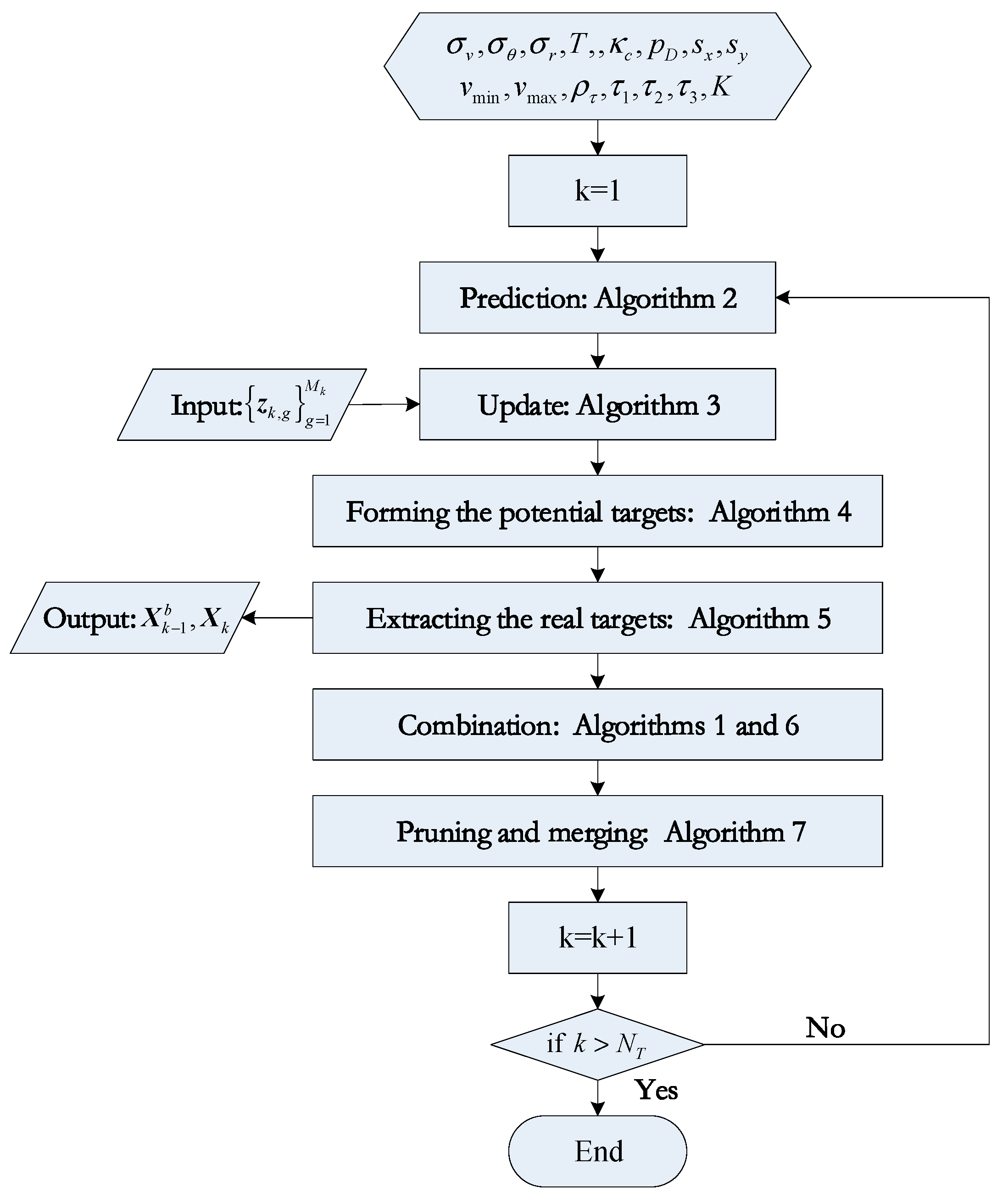
The flowchart of the AMHMB filter is given in Figure 1, where $N_T$ denotes the maximum recursion number.

To form the PDFs and existence probabilities of different targets in the recursion, the K-best hypotheses are needed in the proposed AMHMB filter. This filter uses the measurements from time steps $k-1$ and $k$ to form the potential birth objects. The state vectors and covariance matrices for potential birth targets are given adaptively.

5. Simulation Results

In this section, in order to test the tracking performance of the AMHMB filter, the AGLMB filter in [34], the AAMMTB filter in [35], and the adaptive GLMB filter in [30] were selected as the comparison filters. The adaptive GLMB filter in [30] is called the AGLMB1 filter in this article. The original adaptive GLMB filter in [30] uses a robust CPHD filter to estimate the clutter rate (or clutter density) and detection probability. Since the estimations of the clutter rate and detection probability are not involved in this article, prior clutter rate and detection probability are used in the AGLMB1 filter. The fixed prior covariance matrix for the AGLMB1 filter is given as follows:

$${\mathit{P}}_{k,i}^b=\left[\begin{array}{cccc}{\left(30 \mathrm{m}\right)}^2& 0& 0& 0\\ 0& {\left(10 {\mathrm{ms}}^{-1}\right)}^2& 0& 0\\ 0& 0& {\left(30 \mathrm{m}\right)}^2& 0\\ 0& 0& 0& {\left(10 {\mathrm{ms}}^{-1}\right)}^2\end{array}\right]$$

(52)

According to [30], the existence probability of the potential birth object in this adaptive filter is given by the following:

$$r_{k,g}^b=\min \left(r_{\max }^b,\frac{\left(1-p_{{\mathit{z}}_{k,g}}\right){\lambda }_B}{{\displaystyle \sum _{g=1}^{M_k}1-p_{{\mathit{z}}_{k,g}}}}\right)$$

(53)

where $r_{\max }^b$ is the maximum existence probability of a potential birth object, $p_{{\mathit{z}}_{k,g}}$ is the used probability of observation ${\mathit{z}}_{k,g}$, and ${\lambda }_B$ is the expected number of birth targets at time step $k+1$. In the experiment, ${\lambda }_B$ is set to ${\lambda }_B=0.1$, and parameter $r_{\max }^b$ in the AMHMB filter and AGLMB1 filter is set to $r_{\max }^b=0.003$.

The metrics used for evaluating the performance of filters are the OSPA⁽²⁾ distance [37], cardinality error, and performing time. The OSPA⁽²⁾ distance is a metric for evaluating the dissimilarity between two sets of tracks. Let $\mathit{A}=\left\{{\tau }^{\left(1\right)},{\tau }^{\left(2\right)},\cdots .{\tau }^{\left(m\right)}\right\}$ and $\mathit{B}=\left\{{\varsigma }^{\left(1\right)},{\varsigma }^{\left(2\right)},\cdots ,{\varsigma }^{\left(n\right)}\right\}$ denote two sets of tracks. If $m\le n$, the OSPA⁽²⁾ distance between these two sets is as follows:

$$d_{p,q}^{\left(c\right)}\left(\mathit{A},\mathit{B};w\right)={\left(\frac{1}{n}\left(\underset{\pi \in {\Pi }_n}{\min }{{\displaystyle \sum _{i=1}^m{d}_q^{\left(c\right)}\left({\tau }^{\left(i\right)},{\varsigma }^{\left(\pi \left(i\right)\right)};w\right)}}^p+\left(n-m\right)c^p\right)\right)}^{1/p}$$

(54)

where $p$ and $q$ denote the order, ${\prod }_n$ denotes the set $\{1,2,\cdots ,n\}$, and $w$ is a set of weights. If $m>n$, then $d_{p,q}^{\left(c\right)}\left(\mathit{A},\mathit{B};w\right)=d_{p,q}^{\left(c\right)}\left(\mathit{B},\mathit{A};w\right)$. For the OSPA⁽²⁾ distance, the reader may acquire more detail from [37]. In the experiment, the parameters for the OSPA⁽²⁾ distance are set to $p=q=2$, $L_w=5$, and $c=100 \mathrm{m}$, where $L_w$ is the size of $w$.

Cardinality error denotes the difference of object numbers. Its definition is the following:

$$n_e=\frac{{\displaystyle \sum _{i=1}^{N_s}{\displaystyle \sum _{k=1}^{N_T}\left|n_{ik}^E-n_{ik}^T\right|}}}{N_s\times N_T}$$

(55)

where $N_s$ denotes the number of Monte Carlo runs, $N_T$ is the number of time steps, and $n_{ik}^E$ and $n_{ik}^T$ denote the estimated object number and true object number, respectively.

The performing time is the average time required for a Monte Carlo run. Its definition is as follows:

$$T_e={\displaystyle \sum _{i=1}^{N_s}{T}_i}/N_s$$

(56)

where $T_i$ is the time required for Monte Carlo run $i$.

The simulation hardware environment is Lenovo ThinkPad T470, and software environment is Windows 10 and MATLAB R2021b. In the simulation, two scenarios are considered.

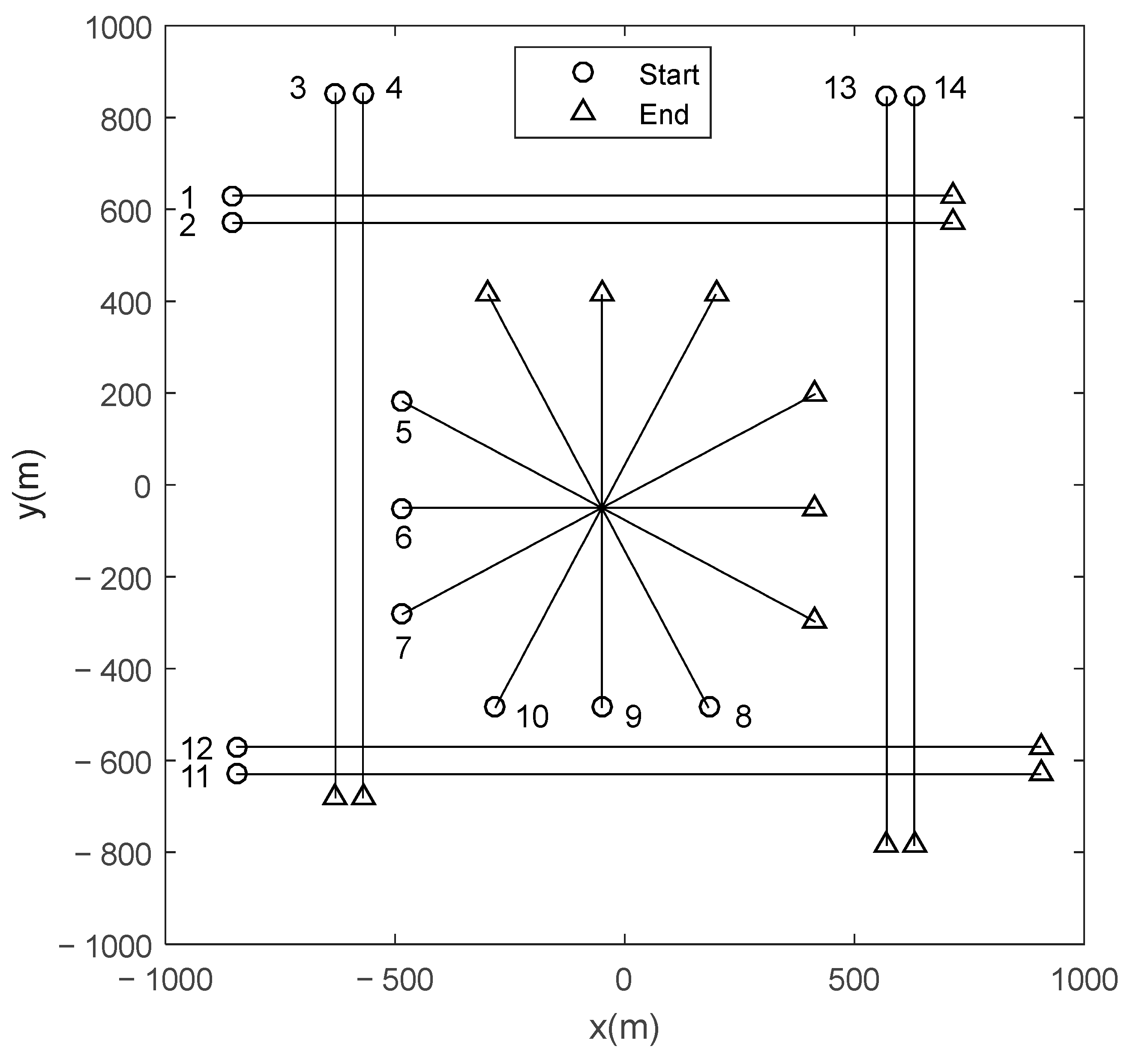
Scenario 1: There are fourteen moving targets in this scenario. Their true tracks are illustrated in Figure 2, and their appearing time, disappearing time, and state vector are given in

Table 1. Appearing times, disappearing times, and initial state vectors of targets.

Target	Appearing Time (s)	Disappearing Time (s)	Initial State
1	1	100	${[-870, 16 , 630, 0 ]}^{\mathrm{T}}$
2	1	100	${[-870, 16 , 570, 0 ]}^{\mathrm{T}}$
3	3	100	${[-630, 0 , 870, -16 ]}^{\mathrm{T}}$
4	3	100	${[-570, 0 , 870, -16 ]}^{\mathrm{T}}$
5	8	68	${[-500, 15 , 190, -8 ]}^{\mathrm{T}}$
6	8	68	${[-500, 15 , -50, 0 ]}^{\mathrm{T}}$
7	8	68	${[-500, 15 , -290, 8 ]}^{\mathrm{T}}$
8	8	68	${[190, -8,-500, 15 ]}^{\mathrm{T}}$
9	8	68	${[-50, 0,-500, 15 ]}^{\mathrm{T}}$
10	8	68	${[ -290, 8,-500, 15 ]}^{\mathrm{T}}$
11	26	100	${[-870, 24 , -630, 0 ]}^{\mathrm{T}}$
12	26	100	${[-870, 24 , -570, 0 ]}^{\mathrm{T}}$
13	31	100	${[630, 0 , 870, -24 ]}^{\mathrm{T}}$
14	31	100	${[570, 0 , 870, -24]}^{\mathrm{T}}$

. The state vector of target $i$ at time step $k$ is ${\mathit{x}}_{k,i}={\left[\begin{array}{cccc}{\zeta }_{k,i}^x& {\dot{\zeta }}_{k,i}^x& {\zeta }_{k,i}^y& {\dot{\zeta }}_{k,i}^y\end{array}\right]}^{\mathrm{T}}$, where ${\zeta }_{k,i}^x$ and ${\zeta }_{k,i}^y$ are the position components, and their unit is m; ${\dot{\zeta }}_{k,i}^x$ and ${\dot{\zeta }}_{k,i}^y$ are the velocity components, and their unit is ms⁻¹.

The fourteen targets move according to (1), and ${\mathit{\Phi }}_{k-1}$ and ${\mathit{Q}}_{k-1}$ in (1) and (35) are given by the following:

$${\mathit{\Phi }}_{k-1}=\left[\begin{array}{cc}\mathit{f}& \mathbf{0}\\ \mathbf{0}& \mathit{f}\end{array}\right]; \mathit{f}=\left[\begin{array}{cc}1& T\\ 0& 1\end{array}\right]$$

(57)

$${\mathit{Q}}_{k-1}=\left[\begin{array}{cc}\mathit{g}& \mathbf{0}\\ \mathbf{0}& \mathit{g}\end{array}\right]; \mathit{g}=\left[\begin{array}{cc}{T}^4/4& T^3/2\\ T^3/2& T^2\end{array}\right]{\sigma }_v^2$$

(58)

where scan period $T=1 \mathrm{s}$, and standard deviation of process noise ${\sigma }_v=2 {\mathrm{ms}}^{-2}$. Random process noise may result in the perturbations of the moving tracks of targets. It can simulate the realistic scenario of target motion.

A radar located at [0, 0]^T observes the fourteen targets moving in the surveillance region. The target-originated observations are generated according to (2), where ${\mathit{R}}_k$ in (2) and (37) is given by the following:

$${\mathit{R}}_k=\left[\begin{array}{cc}{\sigma }_{\theta }^2& 0\\ 0& {\sigma }_r^2\end{array}\right]$$

(59)

Detection probability $p_D=0.9$, average clutter number $N_c=30$ (i.e., average clutter density is ${\kappa }_c=3.3767\times {10}^{-3}{\mathrm{rad}}^{-1}{\mathrm{m}}^{-1}$), and standard deviations of observation noises ${\sigma }_{\theta }=0.3\pi /180\mathrm{rad}$ and ${\sigma }_r=2 \mathrm{m}$ are used to generate simulated measurements. Figure 3 illustrates the simulated observations of a Monte Carlo run, where black dots denote clutter, and red dots denote the target-originated observations. Due to process noise and observation noise, the target-originated observations deviate from the true positions of targets. Some of the target-originated observations are missing by reason of missed detection.

In the experiment, parameters $v_{\min }$ and $v_{\max }$ in (7) are set to $v_{\min }=5{\mathrm{ms}}^{-1}$ and $v_{\max }=50 {\mathrm{ms}}^{-1}$; the number of hypotheses in the AMHMB filter is set to $K=30$, and its other parameters are ${\rho }_{\tau }=0.5$, ${\tau }_1={\tau }_2={10}^{-5}$, and ${\tau }_3=4$; and the other parameters of the AAMMTB filter, AGLMB filter, and AGLMB1 filter are identical to those in Ref. [35], Ref. [34], and Ref. [22], respectively.

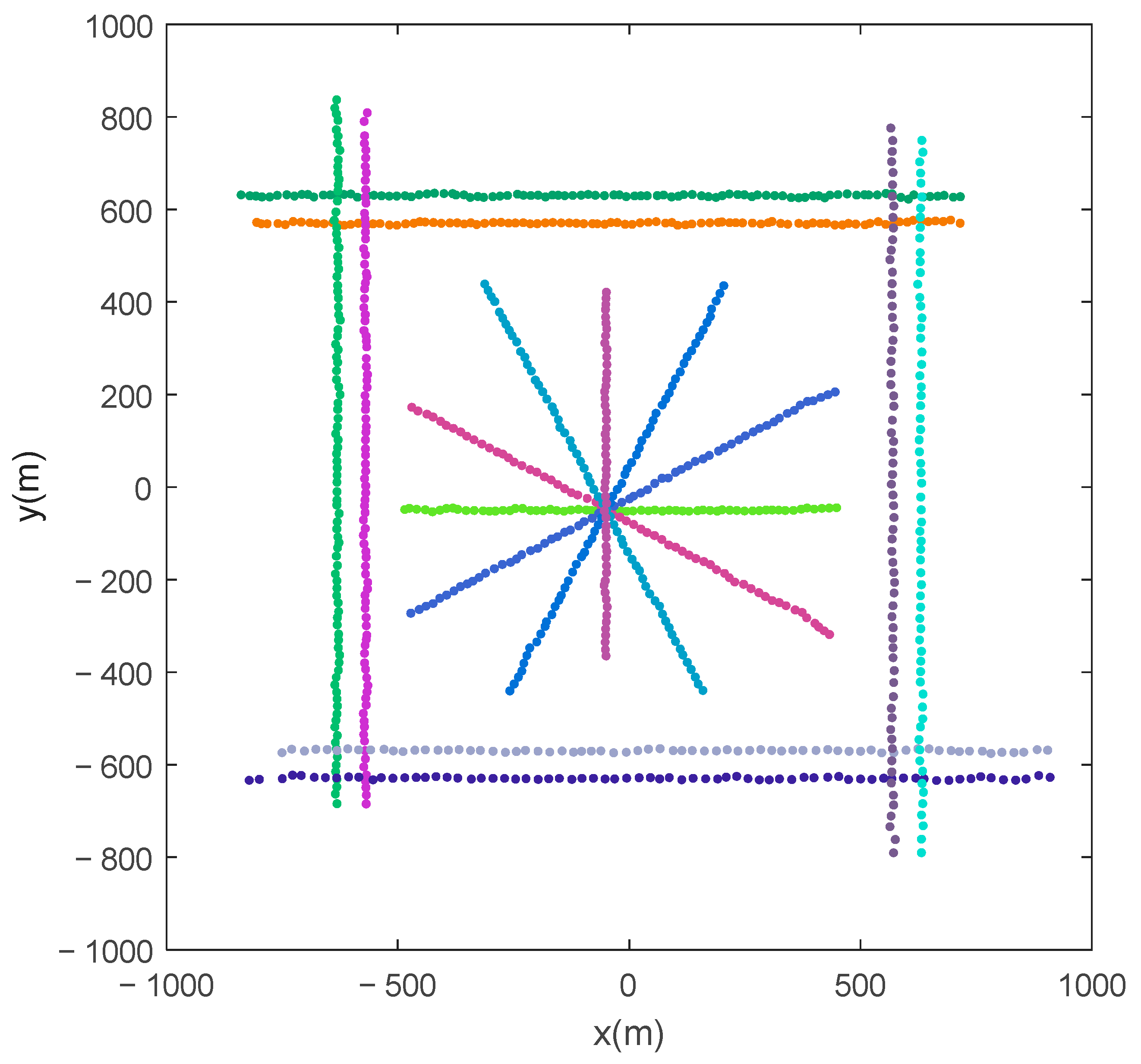
Figure 4 and Figure 5 can be acquired by using the AMHMB filter to handle the simulated measurements in Figure 3. A comparison of Figure 4 with Figure 2 shows that the AMHMB filter can track the fourteen objects, and the estimated target positions approximate the true target positions. A comparison of Figure 4 with Figure 3 shows that clutter is removed by the AMHMB filter, and this filter can provide the state estimation of a target if this target is undetected. 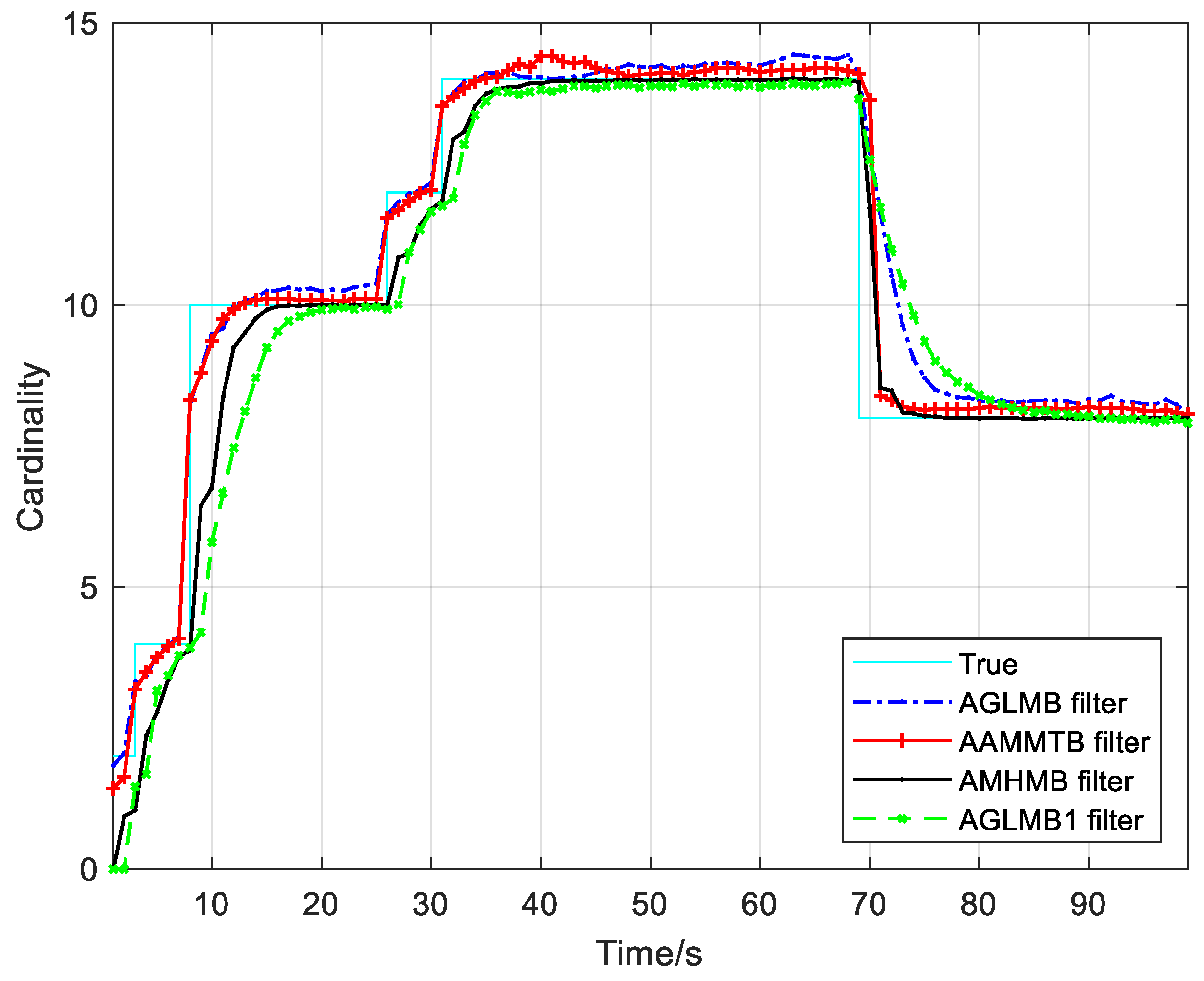Figure 5 indicates that the estimated object number approximates the true object number and also reveals that the AMHMB filter has a delayed response to target appearance and disappearance. The estimated number of targets is less than the number of true targets during target appearing stage and is larger than the number of true targets during target disappearing stage.

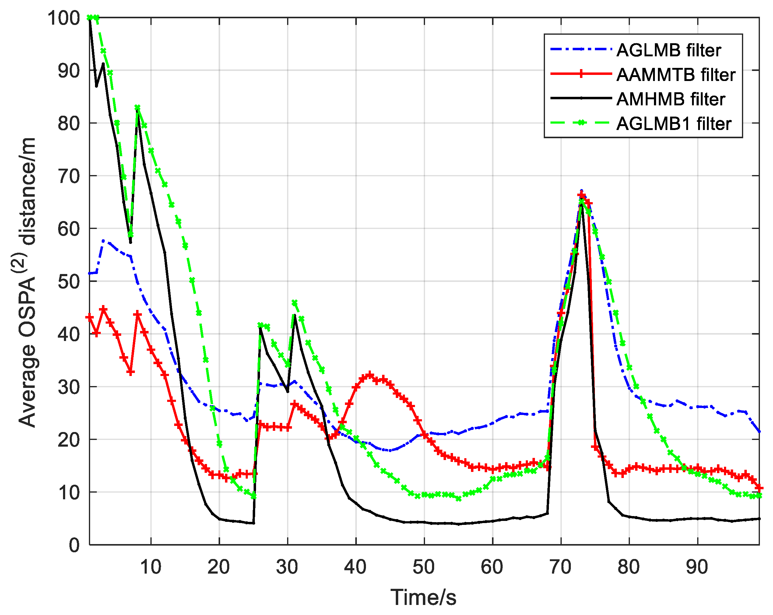
The results from the testing of the AMHMB filter and comparison filters over 250 Monte Carlo runs are given in Figure 6 and Figure 7 as well as

Table 2. Performing time, cardinality error, and OSPA⁽²⁾ distance in scenario 1.

Filter	AAMMTB	AMHMB	AGLMB	AGLMB1
Performing time (s)	0.4174	7.5491	11.0471	106.0145
Cardinality error	0.3283	0.4837	0.4637	0.8292
OSPA(2) distance (m)	22.8887	20.5950	30.7624	31.4417

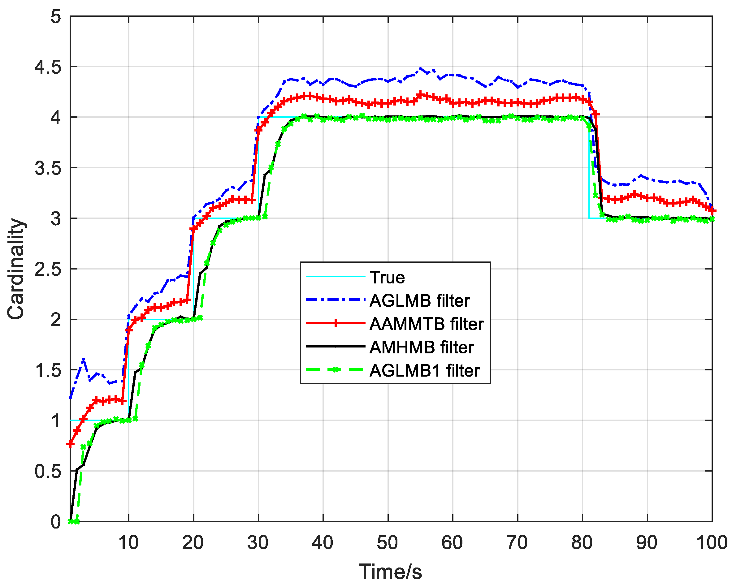
. The OSPA⁽²⁾ distance in Figure 6 and Table 2 shows that the AMHMB filter performs best among these four filters, followed by the AAMMTB filter. The cardinality error in Figure 7 and Table 2 reveals that the AAMMTB filter has a slightly smaller cardinality error than the AMHMB filter. In terms of Figure 6 and Figure 7, the AMHMB filter shows a lower performance than the AAMMTB filter during the target appearing stage. This is because the AAMMTB filter has a more rapid response to target appearance than the AMHMB filter. The AMHMB filter requires more time steps to detect a new target. The performing time in Table 2 indicates that the computational load of the AAMMTB filter is the least. This is because the AAMMTB filter requires only an optimal assignment in each recursion, whereas the other three filters need multiple hypotheses in the recursion. According to Table 2, the computational cost of the AMHMB filter is moderate: larger than that of the AAMMTB filter and smaller than that of other two filters.

To test the robustness, different detecting probabilities, different noisy standard deviations, and different clutter densities are used to generate the simulated observations. The tracking results over 50 Monte Carlo runs for each case are given in

Table 3. Effect of detection probability in scenario 1 ($N_c=30$, metric: OSPA⁽²⁾).

${\mathit{p}}_{\mathit{D}}$	AAMMTB	AMHMB	AGLMB	AGLMB1
1.00	12.8472	16.0359	23.8268	24.3328
0.95	18.2578	19.0762	26.5855	27.0847
0.90	23.3070	20.5934	31.0667	31.4645
0.85	24.8255	22.6114	32.3074	32.8467
0.80	29.9138	26.0055	35.2783	35.4145
0.75	31.5685	26.9511	38.0324	37.1923
0.70	36.3618	30.1409	40.2556	40.3772

,

Table 4. Effect of noisy deviation in scenario 1 ($N_c=30$, $p_D=0.9$, metric: OSPA⁽²⁾).

${\mathit{\sigma }}_{\mathit{r}}$ (m)	${\mathit{\sigma }}_{\mathit{\theta }}$ (°)	AAMMTB	AMHMB	AGLMB	AGLMB1
2	0.2	23.1841	22.4098	29.6170	37.2219
3	0.3	26.8622	21.1901	30.5717	28.8806
4	0.4	32.3723	23.7437	32.8860	29.8464
5	0.5	35.9085	24.8114	34.9409	30.5292
6	0.6	40.7157	25.6378	37.9174	30.9369
7	0.7	45.4473	26.8360	41.6830	31.7840

and

Table 5. Effect of clutter density in scenario 1 ($p_D=0.9$, metric: OSPA⁽²⁾).

${\mathit{N}}_{\mathit{c}}$	${\mathit{\kappa }}_{\mathit{c}}\mathbf{(}{\mathbf{rad}}^{-1}{\mathit{m}}^{-1}\mathbf{)}$	AAMMTB	AMHMB	AGLMB	AGLMB1
10	$1.1256\times {10}^{-3}$	15.4344	18.4650	19.1980	27.8230
15	$1.6883\times {10}^{-3}$	15.4193	18.9202	19.6513	27.8275
20	$2.2511\times {10}^{-3}$	18.8158	19.7472	23.5485	29.5041
25	$2.8139\times {10}^{-3}$	20.4935	19.8512	26.9792	30.6442
30	$3.3767\times {10}^{-3}$	22.6925	20.3510	30.4676	30.6164
35	$3.9395\times {10}^{-3}$	26.5639	21.0144	35.6531	31.9153
40	$4.5023\times {10}^{-3}$	29.7954	21.5778	38.3025	32.8180

, which indicate that the AMHMB filter is the best in most cases. As shown in Table 3 and Table 5, its OSPA⁽²⁾ distance is slightly larger than that of AAMMTB filter at $p_D=1.0$ and $p_D=0.95$ as well as $N_c=10$, $N_c=15$, and $N_c=20$. Two reasons may be the cause of this phenomenon. The first is that the AAMMTB filter has a more rapid response to target appearance than the AMHMB filter. The second is that the accuracy of the data association of the AAMMTB filter is improved significantly under conditions of low clutter density and high detection probability. The experimental results indicate that the AMHMB filter is robust. Unlike the AAMMTB filter that requires a low clutter density and a high detection probability, the AMHMB filter obviates this requirement. It performs better at high clutter densities and low detection probabilities than other adaptive filters.

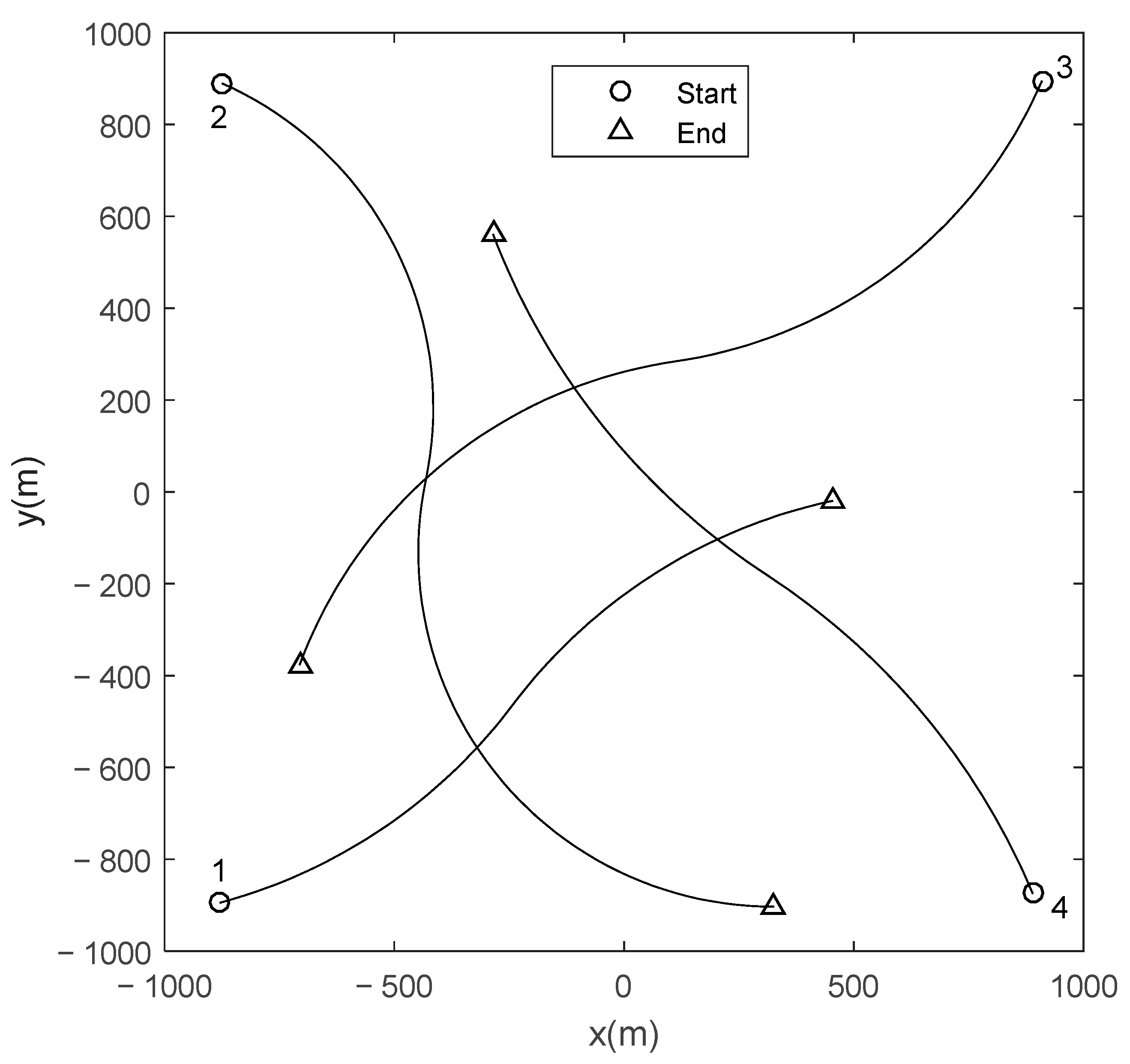
Scenario 2: To test the performance of the AMHMB filter on tracking the maneuvering target, four turn-maneuvering targets are considered in scenario 2. The initial states of targets 1, 2, 3, and 4 are [−900, 20, −900, 5]^T, [−900, 25, 900, −10]^T, [920, −10, 920, −25]^T, and [900, −10, −900, 25]^T, respectively. They appear at t = 1 s, t = 10 s, t = 20 s, and t = 30 s and disappear at t = 80 s, t = 101 s, t = 101 s, and t = 101 s, respectively. Their initial turn rates are ${\omega }_1=0.0174$ rads⁻¹, ${\omega }_2=0.0348$ rads⁻¹, ${\omega }_3=0.0261$ rads⁻¹, and ${\omega }_4=0.0174$ rads⁻¹, respectively. These four targets change their turn rates from ${\omega }_i$ to $-{\omega }_i$ at t = 40 s, t = 50 s, t = 60 s, and t = 65 s, respectively, where $i=1,2,3,4$. 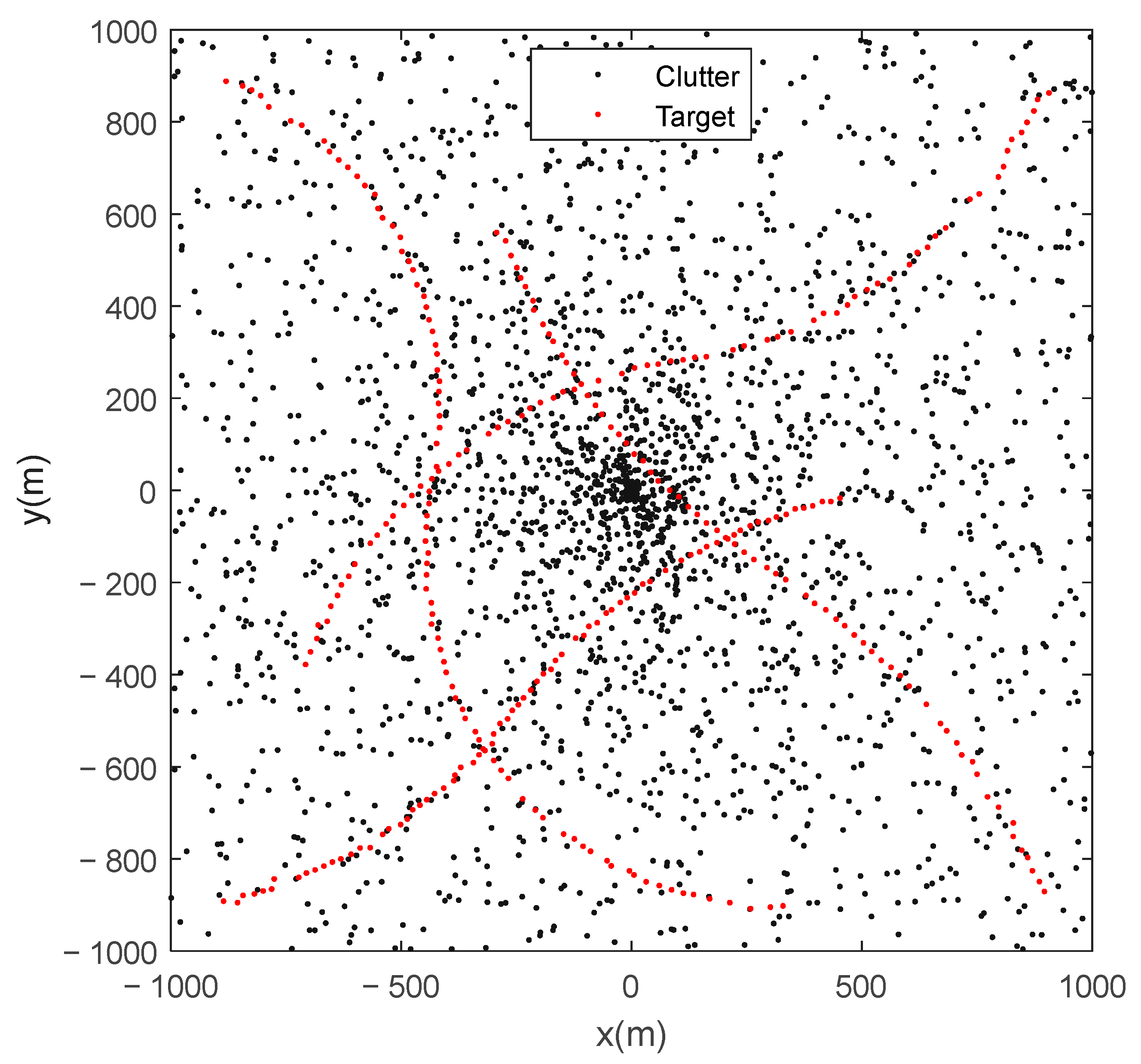The true trajectories of the four maneuvering targets are given in Figure 8. Using process noise ${\sigma }_v=2{\mathrm{ms}}^{-2}$, detection probability $p_D=0.9$, average clutter number $N_c=30$ (i.e., average clutter density is ${\kappa }_c=3.3767\times {10}^{-3}{\mathrm{rad}}^{-1}{\mathrm{m}}^{-1}$), and standard deviations of observation noises ${\sigma }_{\theta }=0.3\pi /180\mathrm{rad}$ and ${\sigma }_r=2 \mathrm{m}$ to generate simulated measurements, the simulated observations of a Monte Carlo run are given in Figure 9, where black dots denote clutter, and red dots denote the target-originated observations. Due to process noise and observation noise, the target-originated observations deviate from true positions of targets. Some of target-originated observations are missing by reason of missed detection.

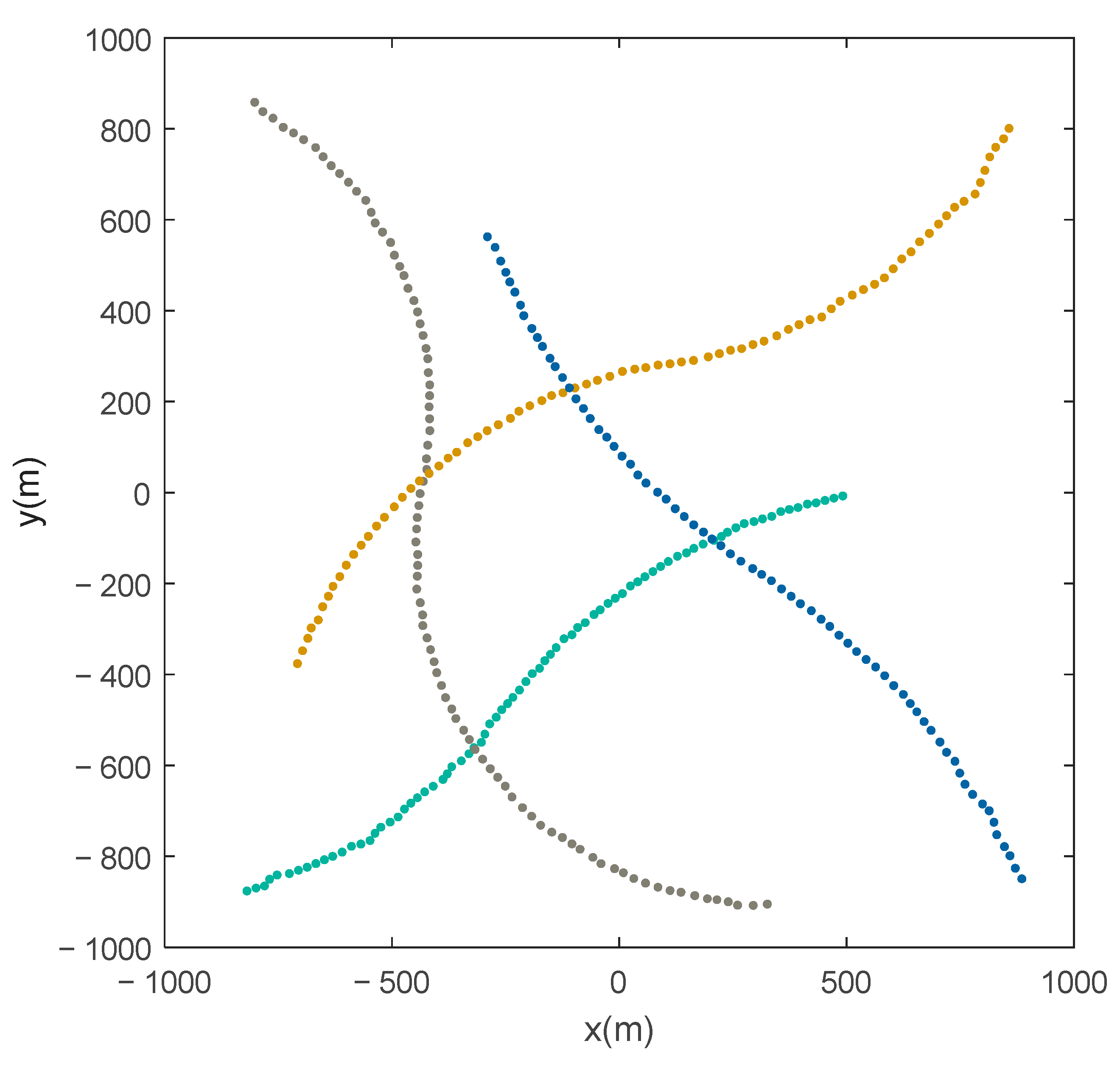
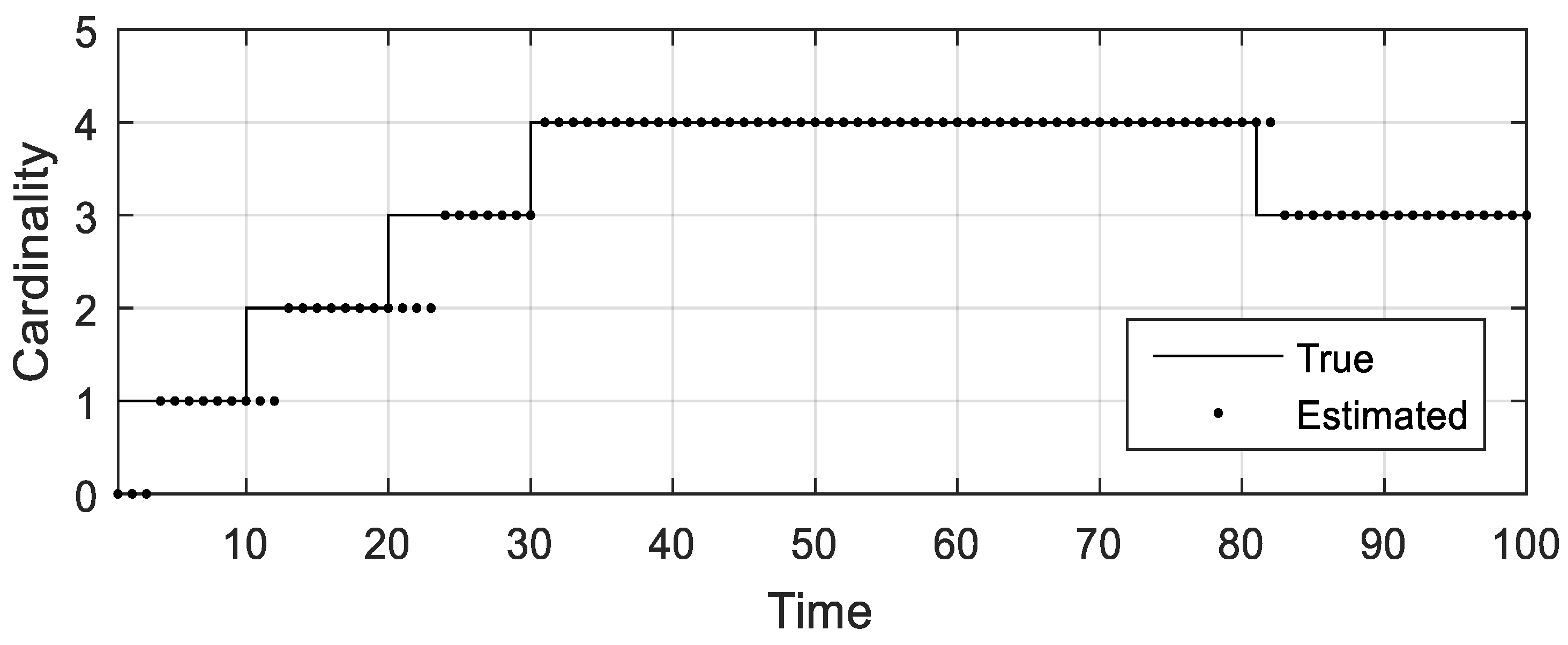
Figure 10 and Figure 11 can be acquired by using the AMHMB filter to handle the simulated measurements in Figure 9. A comparison of Figure 10 with Figure 8 shows that the AMHMB filter can track the four maneuvering targets in the presence of missed detection, clutter, and noise. Figure 11 indicates that it may provide an accurate estimation of object number. Figure 11 also reveals that two to four time steps are required for the AMHMB filter to start tracking a new target.

The tracking result (over 250 Monte Carlo runs) in Figure 12 and Figure 13 as well as

Table 6. Performing time, cardinality error and OSPA⁽²⁾ in scenario 2.

Filter	AAMMTB	AMHMB	AGLMB	AGLMB1
Performing time (s)	0.4459	3.9138	4.2566	66.2809
Cardinality error	0.1731	0.1197	0.3399	0.1345
OSPA(2) distance (m)	23.5526	19.6693	38.8377	23.7067

indicates that the OSPA⁽²⁾ distance and cardinality error of the AMHMB filter are the least among these four filters, and its computational load is moderate: larger than that of the AAMMTB filter and smaller than that of other two filters. Compared with the OSPA⁽²⁾ distance of the AAMMTB filter, the OSPA⁽²⁾ distance of the AMHMB filter is reduced by 16% in terms of Table 6.

Different detecting probabilities, different noisy standard deviations, and different clutter densities were used to test the robustness. The tracking results over 50 Monte Carlo runs for each case are given in

Table 7. Effect of detection probability in scenario 2 ($N_c=30$, metric: OSPA⁽²⁾).

${\mathit{p}}_{\mathit{D}}$	AAMMTB	AMHMB	AGLMB	AGLMB1
1.00	12.8472	16.0359	23.8268	24.3328
0.95	18.2578	19.0762	26.5855	27.0847
0.90	23.3070	20.5934	31.0667	31.4645
0.85	24.8255	22.6114	32.3074	32.8467
0.80	29.9138	26.0055	35.2783	35.4145
0.75	31.5685	26.9511	38.0324	37.1923
0.70	36.3618	30.1409	40.2556	40.3772

,

Table 8. Effect of noisy deviation in scenario 2 ($N_c=30$, $p_D=0.9$, metric: OSPA⁽²⁾).

${\mathit{\sigma }}_{\mathit{r}}$ (m)	${\mathit{\sigma }}_{\mathit{\theta }}$ (°)	AAMMTB	AMHMB	AGLMB	AGLMB1
2	0.2	21.9940	19.6437	37.9552	27.7761
3	0.3	32.6734	20.7196	38.3731	24.5702
4	0.4	38.5794	23.6992	40.7337	24.6653
5	0.5	43.0388	24.4145	41.3564	25.9202
6	0.6	51.7058	25.3075	42.7738	26.4157
7	0.7	57.3209	26.8953	43.5881	28.4108

and

Table 9. Effect of clutter density in scenario 2 ($p_D=0.9$, metric: OSPA⁽²⁾).

${\mathit{N}}_{\mathit{c}}$	${\mathit{\kappa }}_{\mathit{c}}\mathbf{(}{\mathbf{rad}}^{-1}{\mathit{m}}^{-1}\mathbf{)}$	AAMMTB	AMHMB	AGLMB	AGLMB1
10	$1.1256\times {10}^{-3}$	10.6005	17.3686	15.1412	21.0531
15	$1.6883\times {10}^{-3}$	11.7021	17.4748	16.1928	21.9788
20	$2.2511\times {10}^{-3}$	16.9173	19.0626	25.3731	23.5803
25	$2.8139\times {10}^{-3}$	19.7829	19.5819	30.9758	24.1632
30	$3.3767\times {10}^{-3}$	24.3955	20.4220	39.9325	24.7812
35	$3.9395\times {10}^{-3}$	29.0506	20.9678	47.6558	23.2805
40	$4.5023\times {10}^{-3}$	33.8732	20.4852	52.9346	24.5429

. Conclusions identical to scenario 1 can be drawn according to Table 7, Table 8 and Table 9. The AMHMB filter is the best in most cases. The AAMMTB filter performs better than the AMHMB filter under conditions of low clutter density and high detection probability. The AMHMB filter performs better at high clutter densities and low detection probabilities than other adaptive filters.

Effect of $K$: Different values of $K$ are used in the AMHMB filter to test the effect of the number of hypotheses on its performance.

Table 10. Effect of $K$ ($N_c=30$ and $p_D=0.9$).

$\mathit{K}$		5	20	30	50	100
Scenario 1	OSPA(2) distance (m)	22.4659	20.6563	20.2936	20.4208	20.3918
	Performing time (s)	4.5022	6.8250	8.1444	10.5500	16.0416
Scenario 2	OSPA(2) distance (m)	20.3999	20.3546	20.3546	20.3546	20.3546
	Performing time (s)	2.4847	3.9650	4.2213	4.8484	6.1481

shows the OSPA⁽²⁾ distances and performing times over 50 Monte Carlo runs in scenario 1 and scenario 2. According to Table 10, a large value of $K$ leads to the increase of the computational load, and the OSPA⁽²⁾ distance is the smallest at $K=30$. The suggested value of $K$ is $K\ge 20$ in terms of Table 10.

Effect of $r_{\max }^b$: Different values of $r_{\max }^b$ were used in the AMHMB filter to test the effect of the maximum existence probability on its performance.

Table 11. Effect of $r_{\max }^b$ ($N_c=30$, $p_D=0.9$, and $K=30$).

${\mathit{r}}_{\mathbf{max}}^{\mathit{b}}$		0.05	0.01	0.005	0.003	0.001
Scenario 1	OSPA(2) distance (m)	21.1636	20.0116	20.1412	20.5451	22.8247
	Performing time (s)	9.1484	8.2072	7.9700	7.7956	7.1706
Scenario 2	OSPA(2) distance (m)	22.7577	20.1284	19.5741	19.5850	22.3354
	Performing time (s)	4.9375	4.0378	3.9453	3.8691	2.9688

shows the OSPA⁽²⁾ distances and performing times over 50 Monte Carlo runs in scenario 1 and scenario 2. According to Table 11, the computational load decreases as the value of $r_{\max }^b$ reduces, and the OSPA⁽²⁾ distance is the smallest at $r_{\max }^b=0.01$ in scenario 1 and is the smallest at $r_{\max }^b=0.005$ in scenario 2. The suggested value range of $r_{\max }^b$ is $r_{\max }^b\in [0.003,0.01]$ in terms of Table 11.

Superiority of the birth approach: Replacing the birth approach in the AMHMB filter with the birth approach in the adaptive GLMB filter of [30], an AMHMB1 filter can be established. The main difference between the AMHMB filter and the AMHMB1 filter is that they use the different birth approaches.

Table 12. Effect of the birth approach ($N_c=30$, $p_D=0.9$, and $K=30$).

		AMHMB1 Filter	AMHMB Filter
Scenario 1	OSPA(2) distance (m)	23.9529	20.1518
	Cardinality error	0.5509	0.4653
	Performing time (s)	35.5750	7.7803
Scenario 2	OSPA(2) distance (m)	22.6274	19.2526
	Cardinality error	0.1348	0.1208
	Performing time (s)	30.7697	3.9872

shows the OSPA⁽²⁾ distances, cardinality errors, and performing times over 50 Monte Carlo runs in scenario 1 and scenario 2, which reveals that the OSPA⁽²⁾ distances, cardinality errors, and performing times of the AMHMB filter are less than those of the AMHMB1 filter. This result also indicates the use of the birth approach proposed in this article improves the tracking accuracy and decreases the computational load. The reason may be that the proposed birth approach reduces the number of potential birth targets.

Computational complexity: The AMHMB filter has a $\mathcal{O}\left(K{(2N+M)}^3\right)$ computational complexity, where $N$, $M$, and $K$ are the object number, observation number, and hypothesis number, respectively. Reducing the object number and reducing the hypothesis number can decrease the computational cost of the AMHMB filter.

6. Conclusions

An AMHMB filter for tracking multiple targets is proposed in this study. This filter uses the K-best hypotheses to solve the data association problem in MTT to form the PDFs and existence probabilities of potential objects. It uses the observations from two consecutive time steps to generate the state vector and error covariance matrix of the potential birth target adaptively, thereby obviating the requirement for prior state vector and covariance matrix. Experimental results show that the AMHMB filter is robust; its OSPA⁽²⁾ distance is the smallest at most cases; and its computational load is moderate: larger than that of the AAMMTB filter but less than that of other filters. The proposed filter may find its potential applications in real tracking systems, especially in those systems that have a high clutter density and a low detection probability. To solidify the practical utility of this filter in various applications, further research is required in the future.