Article

Scenario-Based Simulation of Impervious Surfaces for Detecting the Effects of Landscape Patterns on Urban Waterlogging

1
Institute of Remote Sensing and Earth Sciences, College of Science, Hangzhou Normal University, Hangzhou 311121, China
2
Zhejiang Provincial Key Laboratory of Urban Wetlands and Regional Change, Hangzhou Normal University, Hangzhou 311121, China
3
Zhejiang Key Laboratory of Safety Engineering and Technology, Zhejiang Academy of Emergency Management Science, Hangzhou 310061, China
*
Author to whom correspondence should be addressed.
Remote Sens. 2024, 16(12), 2130; https://doi.org/10.3390/rs16122130
Submission received: 16 April 2024 / Revised: 7 June 2024 / Accepted: 8 June 2024 / Published: 12 June 2024

Abstract

:
With the increase in global extreme climate events, the frequency of urban waterlogging caused by extreme rainstorms is increasing, resulting in serious economic losses and risk to local residents. Understanding the influence of impervious surfaces on urban waterlogging is of great significance for reducing urban waterlogging disasters. Based on InfoWorks ICM, the urban waterlogging model of Lin’an City was established, and the multi-scenario design method was used to analyze the characteristics and causes of urban waterlogging under different designed rainfall return periods. The results show that the maximum stagnant water depth and area are positively correlated with the proportion of impervious surfaces and rainfall return periods. In addition, urban waterlogging is related to the fragmentation of impervious surfaces, pipeline network, and so on. Based on the findings, it is suggested that impervious surfaces should be placed upstream and along roads where feasible. It is also recommended that the aggregation of impervious surfaces is minimized to prevent urban waterlogging. The results provide technical support and reference for local governments to prevent waterlogging disasters.

Graphical Abstract

1. Introduction

Urbanization is a world-wide outcome of human activities and an inevitable result of the continuous development of economy, culture, and society [1,2]. At present, more than half of the global population resides in urban areas, and this proportion is expected to increase to 70% by the middle of the 21st century [3,4,5]. In the past few decades, developing countries have experienced rapid urbanization [6]. By 2015, the urban population in developing countries accounted for more than 75% of the world’s total urban population [6]. At present, 27 of the world’s 33 megacities are located in developing countries [6]. Urbanization still has strong momentum in the 21st century [7]. As the largest developing country, China is already in the forefront of the world in terms of urban population growth. Since the beginning of the 21st century, China’s urbanization has expanded rapidly, making a significant contribution to social and economic development [8]. From 2000 to 2020, China’s urbanization rate increased from 28% to 64%. Meanwhile, China has become the second largest economy of the world in 2010 [9]. Urbanization is considered to be the most important driver of climate change and has caused many environmental problems, such as urban heat island, air pollution, seawater backflow, and deforestation. Among them, urban waterlogging has been particularly serious in recent years [10,11].
Climate change is one of the greatest environmental challenges for mankind in the 21st century [12]. The intensity and frequency of extreme weather and climate events have increased rapidly in recent years. Events such as rainstorms, high temperatures, heat waves, cold waves, strong winds, and drought have destroyed the ecological environment and caused economic losses [13,14]. Recent statistics have revealed that the frequency and intensity of extreme rainstorm events show a significant upward trend [9]. Urban waterlogging is one of the major disasters caused by extreme rainstorms, affecting socio-economic stability and hindering the United Nations’ sustainable development goals [15]. In recent years, urban waterlogging caused by extreme rainstorms has become more and more frequent. In July 2021, Europe experienced unprecedented torrential rains. This caused severe flooding, damaged infrastructure, disrupted communication networks, and caused serious urban waterlogging [16]. Similarly, in July 2021, torrential rains with a maximum intensity of 201.9 mm per hour occurred in Henan Province, causing devastating urban waterlogging [17]. In the same year, the United States was hit by torrential rains which occur once every 500 years and are caused by hurricanes, causing severe urban waterlogging and subway flooding.
Urban waterlogging is characterized by spatial heterogeneity [18]. An urban waterlogging model is an effective method to simulate the urban waterlogging process and study the mechanism of urban waterlogging disasters [18,19,20]. The existing urban waterlogging hydrological models can calculate the yield and confluence of sub-catchments according to different parameters [19]. Many types of software, including ILLUDAS (Illinois Urban Drainage Area Simulation), SWMM (Storm Water Management Model), HEC-RAS (Hydrological Engineering Center, River Analysis System), LISFLOOD, MIKE FLOOD, and Mike URBAN, are used to simulate urban waterlogging [21]. Developed by the Environmental Protection Agency of the United States, SWMM is completely open-source software and is widely used to simulate urban rainfall–runoff processes [22,23,24]. However, the SWMM model has significant uncertainty and cannot simulate the two-dimensional (2D) overflow process of pipeline overloading [21]. Mike series models (such as Mike 11/Mike 21) do not allow full coupling. They require the coupling of one-dimensional (1D) models (Mike 11/Mike Urban) and 2D models (Mike 21) [25]. InfoWorks ICM, developed by Wallingford, is a comprehensive watershed drainage system model [26]. It combines the widely used GIS interface, simplifies the operation of urban water cycle simulation, and provides visualization [27]. This model realizes the detailed simulation of coupling 1D pipe network and 2D ground in one software [26]. The numerical simulation combined with InfoWorks ICM ensures higher calculation accuracy and efficiency, and makes the model more realistic and convenient [28,29].
Urbanization makes impervious surfaces continue to increase in area, while an extreme climate makes rainstorms occur frequently. The increase in impervious surfaces reduces the rainwater absorption capacity of urban surfaces [30]. Cities with low surface permeability and insufficient drainage capacity are weak in coping with rainstorms and are thus prone to urban waterlogging during rainstorms [31,32]. Frequent urban waterlogging has caused serious economic losses and casualties, damaged infrastructure and communication networks, and threatened social security [33]. A recent estimate indicates that the number of urban areas affected by waterlogging will increase by 2.7 times by 2030 [34]. Globally, the intensity and frequency of urban waterlogging will increase due to changes in precipitation patterns caused by climate change and accelerated urban expansion [35,36]. According to China’s annual report on floods and droughts, urban waterlogging caused huge economic losses every year during the period from 2008 to 2018 [37]. In order to alleviate the problem of urban waterlogging and promote urban waterlogging control, the Chinese government issued the Action Plan for the Construction of Urban Drainage and Waterlogging Prevention System as part of the 14th Five-Year Plan. In this context, urban waterlogging is a serious problem that needs to be solved urgently at present. How to simulate the process of urban waterlogging scientifically and put forward a reasonable and effective mitigation plan is a key issue for sustainable development.
Therefore, in this study, an urban waterlogging model in Lin’an City based on InfoWorks ICM was established. A variety of impervious surface distribution scenarios were designed to explore the influence of the proportion and distribution of impervious surfaces on urban waterlogging. The specific research objectives are as follows: (1) to detect the effect of the proportion of impervious surfaces changes on urban waterlogging; (2) to analyze the impact of spatial distribution changes on urban waterlogging; and (3) to put forward urban waterlogging optimization suggestions based on a comparison of various optimization plans.

2. Materials and Methods

2.1. Study Area

Lin’an District is located in the Tianmu Mountain area, northwest of Hangzhou, Zhejiang Province (Figure 1). The total area of this region is 3118.72 km2. By the end of 2022, the total population was 542,990 [38]. Its geographical coordinates range from 29°56′ to 30°23′N and 118°51′ to 119°52′E. Lin’an District is situated on the southern edge of the subtropical monsoon climate zone in Central Asia, enjoying a warm and humid climate. The region experiences plentiful rainfall and distinct seasons. The terrain slopes from northwest to southeast, surrounded by mountains on the north, west, and south sides. In the northwest of Lin’an District, there are high mountains and deep valleys. The southeast features hills and wide valleys with relatively flat terrain, forming a horseshoe-shaped barrier in the southeastern region. Moist air from the southeast coast cools adiabatically and condenses into precipitation here. Lin’an District frequently experiences urban waterlogging, resulting in significant economic losses and posing a threat to the life and property of its residents. For example, in June 2015, Lin’an District encountered short-term heavy rainfall, causing the collapse of 91 houses and resulting in a total direct economic loss of over 180 million yuan.

2.2. Data Collection and Processing

2.2.1. Data Sources and Pre-Processing

Basic geographic data (see Table 1) includes multi-temporal high-resolution remote sensing images, terrain data, and pipeline network data. The multi-temporal high-resolution remote sensing images were obtained from Google Earth and UAV imaging. Terrain data were sourced from the Surveying and Mapping Department of Lin’an, provided as a raster file with a spatial resolution of 2 m after processing. Pipeline network data were acquired from the Urban Administration of Lin’an, encompassing node data and pipeline data. Historical rainfall data originated from the National Meteorological Science Data Center “http://data.cma.cn/” (accessed on 30 May 2024).
This study primarily selected multi-temporal high-resolution remote sensing images with similar seasons and less cloud cover. These images were projected into CGCS2000_3_Degree_Gauss_Kruger_CM_120E, then cropped according to the boundary of the study area. Land use information was obtained through artificial visual interpretation. In this study, surfaces were divided into three land use types: road, natural surfaces, and impervious surfaces. The generalization method for the pipeline network data was to merge pipelines with the same diameter in areas with dense pipelines and delete or retain rainwater nodes in the pipe network as needed.

2.2.2. Designed Rainfall Events

In order to analyze the influence of the proportion and spatial distribution of impervious surfaces on urban waterlogging, a variety of rainfall scenarios were designed. The commonly used rain pattern analysis methods include the constant method, triangulation method, Desbordes method, Chicago method, West Sifalda method, and soil and water conservation service humidity method [39]. The Chicago rain pattern is a non-uniform-design rain pattern designed by Keifer and Chu in 1957, according to the relationships within the rainfall intensity–duration–frequency curve [40]. The Chicago rainfall pattern is a single-peak rainfall process; the variation in rainfall on both sides of the peak is basically symmetrical. The peak rainfall is determined by the return period and duration. The rainfall process of the Chicago rain pattern with the same total value is more continuous compared to other rainfall patterns. In the case of a short duration and long return period, the frequency of rainfall events is low, and the total rainfall and peak rainfall are large. Compared with the actual peak rainfall process, the characteristics of single-peak and rapid fluctuations are similar to those of disastrous heavy rainstorms. The Chicago method is widely used in rain pattern analyses because of its high accuracy and universality [41,42]. The designed rainfall of this study combines the rainstorm intensity formula of Lin’an City and the Chicago rain pattern. Based on the rainfall data from the national basic weather station in Lin’an City from 1980 to 2015 and using the Pearson type III curve method, the latest rainstorm intensity formula in Lin’an City was obtained [43].
The rainstorm intensity formula in Lin’an City is shown in Equation (1):
q = 2763.132   × 1 + 0.399 lg P t + 10.870 0.753
where q is the intensity of the designed rainstorm in L/(s × hm2); t is the rainfall duration in min; P is the design return period in years.
The designed rainfall return periods of this study were 1-year, 3-year, 5-year, 10-year, and 20-year periods. The related research shows that the rainfall peak coefficient in most areas is between 0.3 and 0.5 [22]. As a result, the rain peak coefficient in this paper is set to 0.4. The peak discharge of a uniform-design rainstorm decreases with the extension of duration and reaches the maximum when the duration is 2 h [43]. As a result, the rainfall duration is set to 2 h. Meanwhile, the best recording interval in a duration of 1–3 h is 5 min, so the rainfall interval in this paper is set to 5 min [44]. A hyetograph of the designed rainfall events is shown in Figure 2.

2.3. Overall Flow

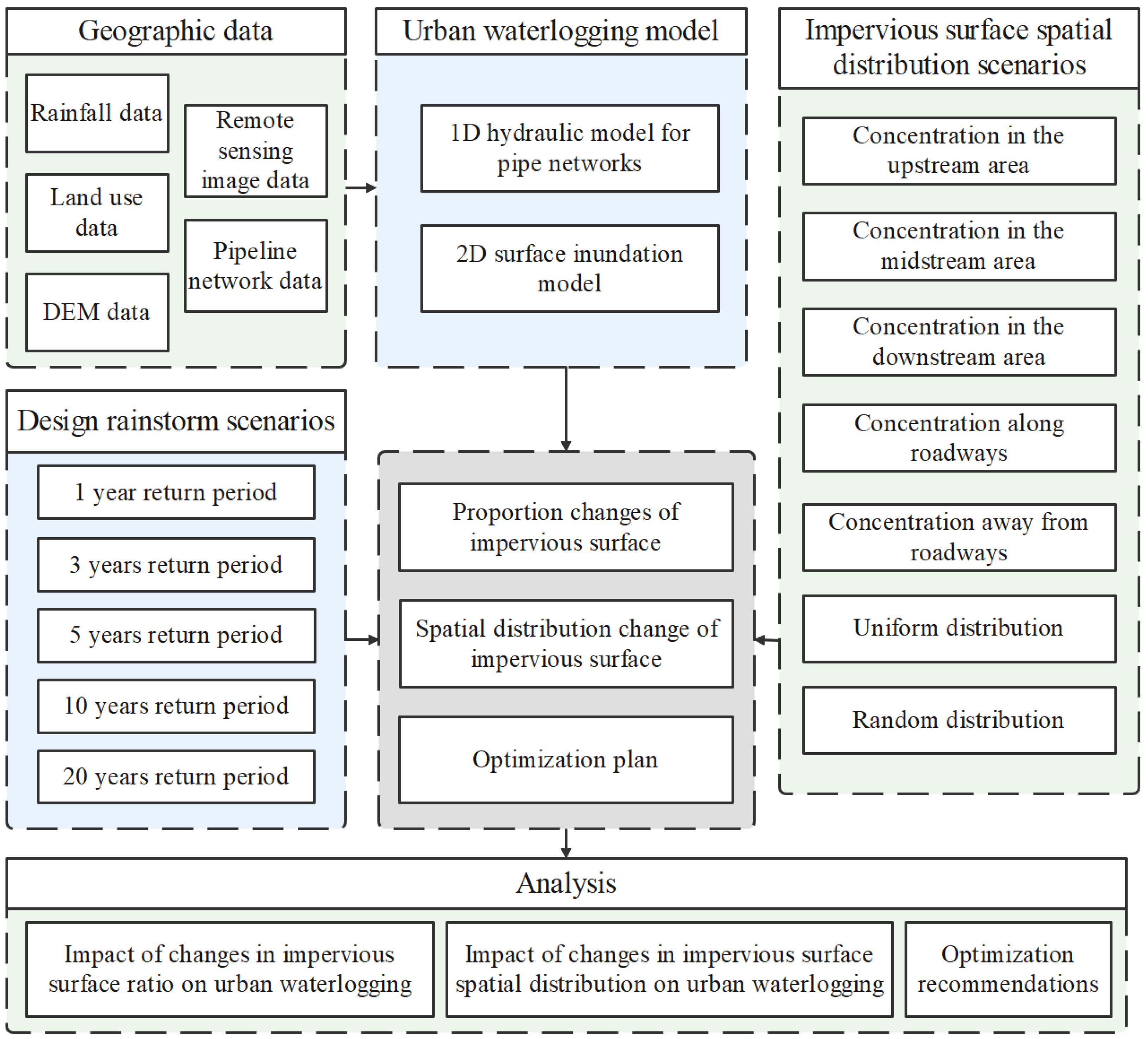
The overall workflow is shown in Figure 3. The whole process can be summarized into five main steps:
(1) The 1D pipe network hydraulic model and the 2D surface inundation model were integrated to construct the urban waterlogging model based on InfoWorks ICM.
(2) Five rainfall events in different return periods were designed by using the rainfall intensity formula in Lin’an City. The designed rainfall events in different return periods and the land use were input into the waterlogging model to analyze the relationship between the impervious surface ratio and various urban waterlogging process parameters.
(3) Based on the ratio of impervious surfaces in 2022, three sets of scenarios with seven different impervious surface spatial distributions were designed. The waterlogging process was simulated, and the impact of changing impervious surfaces distribution on urban waterlogging was analyzed.
(4) According to the results of different distribution impervious surface scenarios, the scenarios with better results from the perspective of stagnant water area and depth in each group were selected. Using the 2022 spatial pattern as a reference, four optimization plans for impervious surface distribution were designed according to the selected scenarios.
(5) The impact of each optimization plan on urban waterlogging was evaluated based on the results of stagnant water area and depth under different return periods. Each optimization plan was compared from the perspective of alleviating waterlogging. Optimization recommendations for impervious surfaces and urban waterlogging disaster management were proposed based on the optimization plans.

2.4. Model Construction

InfoWorks ICM incorporates the hydraulics and hydrology of natural watersheds and man-made environments into a single integrated model [45]. InfoWorks ICM can simulate the urban stormwater circulation process and the working conditions of the stormwater and sewerage systems [46]. InfoWorks ICM has flexible data exchange ability and parallel computing ability, this greatly improves the simplicity and computational efficiency of 2D hydrodynamic simulation [47]. InfoWorks ICM has a hydrological production and confluence model, 1D drainage network model, and 2D surface inundation model. In the pipe network hydrology module, the fully solved Saint-Venant equation is used to simulate open channel flow, and the Preissman method is used to simulate the overload of an open channel [48].
The Saint-Venant equation formula is shown in Equations (2) and (3).
A t + Q x = 0
Q t + x Q 2 A + g A cos θ h x S 0 + Q Q K 2 = 0
where Q is the flow rate in m3/s; A is the cross-sectional area of the pipeline in m2; t is the time in s; x is the length of the pipe along the direction of the current in m; h is the water depth in m; g is the gravity acceleration in m/s2; θ is the horizontal angle in degrees; K is the water transport rate, which is determined by Colebrook–White or Manning formula; and S 0 is the slope at the bottom of the pipe.
The 2D surface inundation model uses the 2D finite volume method to solve shallow flow equations. The Rienmann solver and TVD (Total Variation Diminishing) excitation techniques are used to solve the model [49,50,51]. The 2D surface inundation model is used to simulate the stagnant water flow generated by the drainage network system when passing through the complex geometric terrain. On this basis, the flow velocity, direction, and depth of the flow are obtained. The mathematical expressions for the shallow water flow equations used in InfoWorks ICM are shown in Equations (4)–(6) [49].
h t + h u x + h u y = q 1 D
h u t + x h u 2 + g h 2 2 + h u v y = S 0 , x S f , x + q 1 D u 1 D
h v t + y h v 2 + g h 2 2 + h u v x = S 0 , y S f , y + q 1 D v 1 D
where h is the depth of water in m; u and v are the velocity components in x and y directions in m/s; S 0 , x and S 0 , y are the bottom slope components in the x and y directions, respectively; S f , x and S f , y are the friction components in the x and y directions, respectively; q 1 D is the discharge per unit area in m3/s; u 1 D   a n d   v 1 D are velocity components of q 1 D in the x and y directions, respectively, in m/s.
Based on the generalized pipe network nodes, the sub-catchments were divided by the Theissen polygon method. Next, the Area Take Off (ATO) tool in InfoWorks ICM was used to extract the types and proportion of the runoff-producing surfaces in each sub-catchment. The Horton infiltration model was used to calculate runoff production and confluence. The fixed proportion runoff model was used for other runoff production surfaces. The SWMM model was used for the confluence model. The parameters of the three runoff-producing surfaces were shown in Table 2.
To establish the 2D surface inundation model, the elevation points were extracted according to the DEM data. After that, the elevation data were imported into InfoWorks ICM to establish TIN model. Then, the 2D interval was gridded in the study area to generate a triangular mesh with a maximum area of 50 m2 and a minimum area of 25 m2. The road was set as a gridding interval. The maximum grid area was 10 m2, and the minimum grid area was 5 m2. Based on local knowledge, the road elevation was reduced by 0.15 m to simulate the flood discharge effect of the road.

2.5. Scenario Design for the Spatial Distribution of Impervious Surfaces

To facilitate this study, the remaining area was divided into 2 × 2 m grids. This grid size was chosen for its effectiveness in representing trees and streets, matching the narrow width of sidewalks and the canopy of trees [52]. Figure 4 illustrates the outcomes of this division. By adjusting the grid properties, transitions between impervious and natural surfaces were simulated. Referencing the literature, three sets were devised, comprising a total of seven scenarios for impervious surface spatial distribution [53,54,55]. The first set considered the influence of flow direction. The second set considered the distribution of pipe networks and the influence of roads. The third set considered the influence of landscape patterns.
To minimize the impact of changes in the area of impervious surfaces, the 2022 impervious surface rate was utilized in the study area as a benchmark. In 2022, the total impervious surface in the study area covered 33.83 ha, with an impervious surface rate of 66.15%. Excluding main roads, the impervious surface rate of the area was 58.36%. While maintaining the main roads and the pipeline network constant, various scenarios for impervious surface distribution in the remaining areas were introduced. How various spatial distributions of impervious surfaces affect urban waterlogging was explored to identify optimal distribution scenarios.
The first set of scenarios focused on water flow direction. The overall flow of the study area was from east to west, and three distinct scenarios (S1–S3) were created. These scenarios involved concentrating impervious surfaces either upstream, in the middle stream, or downstream. The second set of scenarios explored the impact of the distribution of pipeline networks and roads. The pipelines in the study area were mainly aligned with the roads. Two scenarios (S4 and S5) were developed to represent the impervious surfaces far away from the roads and along the roads, respectively. The third set of scenarios explored the influence of landscape patterns. Two impervious surface spatial distribution scenarios (S6 and S7) were designed, representing uniform distribution and random distribution, respectively.
The designed scenarios were input into the constructed urban waterlogging model and the simulation results from different rainfall return periods were analyzed. The simulation was conducted with a time step of 30 s and a total simulation duration of 360 min. After completion of the simulation, the maximum stagnant water depth and area were calculated for each scenario under different rainfall return periods.

2.6. Optimization Plan for Impervious Surfaces

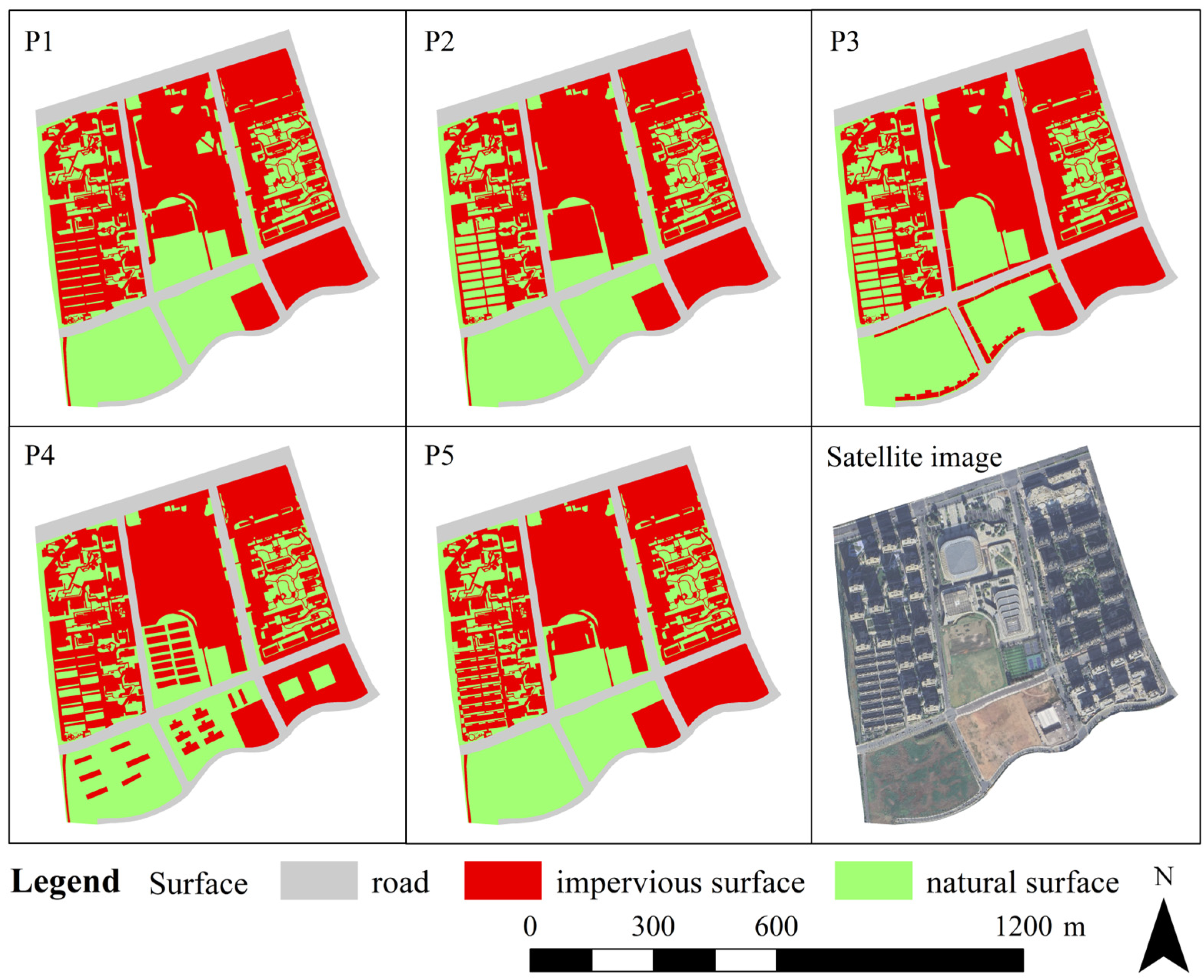
The optimization plans for impervious surfaces were designed based on the spatial distribution of impervious surfaces in 2022 and the simulation results from scenarios of different impervious surface designs. Multiple optimization plans were designed and simulated by moving impervious surface patches, manually drawing features, and modifying patch attributes. The goal was to choose the optimal plan and provide recommendations for optimizing the spatial distribution of impervious surfaces. The principle of the optimization plan design was to reduce the total runoff as much as possible, while keeping the percentage of impervious surfaces in the study area as the actual rate in 2022. The original case in 2022 (P1) and four designed optimization plans (P2-P5) were as follows (Figure 5):
Plan 1 (P1): “Land use in 2022”. P1 was the benchmark plan which was used to compare the design effects of several other optimization plans.
Plan 2 (P2): “Impervious surfaces concentrated upstream”. Based on P1 and the result of the first set of designed scenarios, natural surfaces in the upstream area were converted to impervious surfaces. At the same time, impervious surface patches were added upstream. Part of the impervious surfaces downstream were converted to natural surfaces. As a result, the percentage of impervious surface area in the upper reaches were increased from 56.05% to 60.90%.
Plan 3 (P3): “Impervious surfaces distributed along roads”. Based on P1 and the result of the second set of designed scenarios, part of the impervious surfaces in the western of study area were moved to both sides of the road. As a result, the proportion of impervious surface within 50 m on both sides of the roads were increased from 8.90% to 15.53%.
Plan 4 (P4): “Increase the fragmentation of impervious surfaces”. Based on P1 and the results of the third set of designed scenarios and by drawing impervious surfaces on natural surfaces, the patch configuration was modified to increase the fragmentation of the impervious surfaces. As a result, the division index calculated by Fragstats was increased from 0.9433 to 0.9492.
Plan 5 (P5): “Comprehensive distribution”. Based on P1 and the results of the three sets of designed scenarios, natural surfaces distributed upstream and along the roads were converted to impervious surfaces. Some natural surfaces were added downstream and the fragmentation the impervious surfaces increased. As a result, the impervious area in the upper reaches increased by 4.85%, the division index increased by 0.01%, and the percentage of impervious surfaces distributed along the road increased by 1.153%.

3. Results

3.1. Proportion Changes in Impervious Surfaces

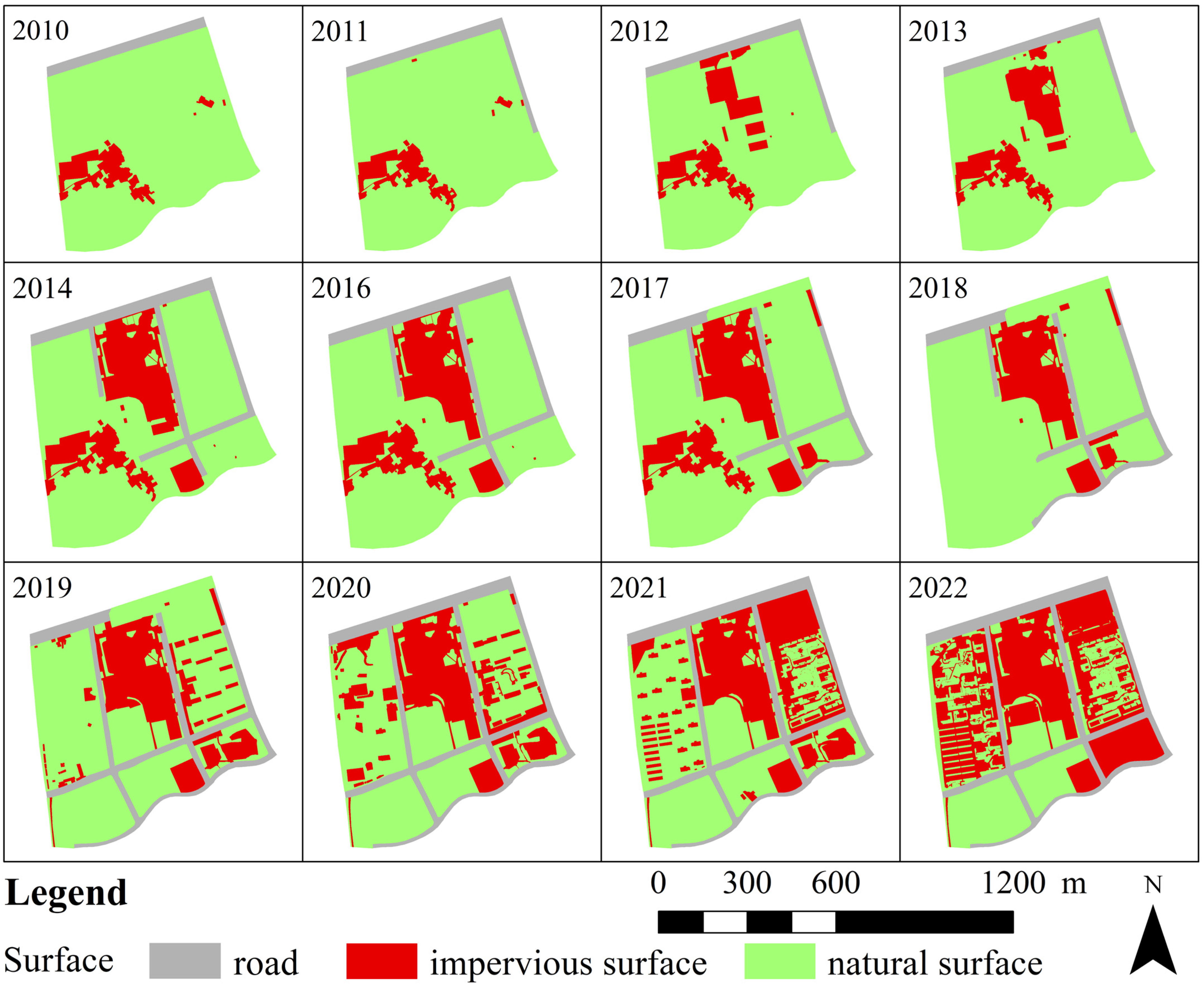
Based on the land use classification of the study area from 2010 to 2022, a map has been generated to illustrate the spatial changes of impervious surfaces over the past 12 years. According to Figure 6, it is evident that the impervious surface ratio in the study area generally shows an increasing trend. However, there was a decrease in impervious surface area in 2017 and 2018. The velocity of change in impervious surfaces varied across different periods, with the fastest occurring between 2021 and 2022.
Table 3 and Figure 7 show the maximum stagnant water depth under different return periods. The range of maximum stagnant water depth spanned from 1.6 cm to 39.6 cm. The highest value of 39.6 cm occurred in the 20-year return period in 2022, and the lowest value of 1.6 cm occurred in the 1-year return period in 2018. In the same return period, an increase in the impervious surface ratio led to a corresponding increase in stagnant water depth. However, the rate of increase varied, with the fastest growth observed in 2022 and the slowest in 2010. The stagnant water area ranged from 1125.50 m2 to 142,068.38 m2, the maximum occurred in the 20-year return period in 2022, and the minimum occurred in the 1-year return period in 2018. Within the same impervious surface ratio, the stagnant water area increased with an extended return period. However, different impervious surface ratio resulted in varying speeds of increase, with the fastest observed in 2021 and the slowest in 2010. Overall, there was a positive correlation among stagnant water depth, stagnant water area, and the impervious surface ratio.

3.2. Spatial Distribution Changes in Impervious Surfaces

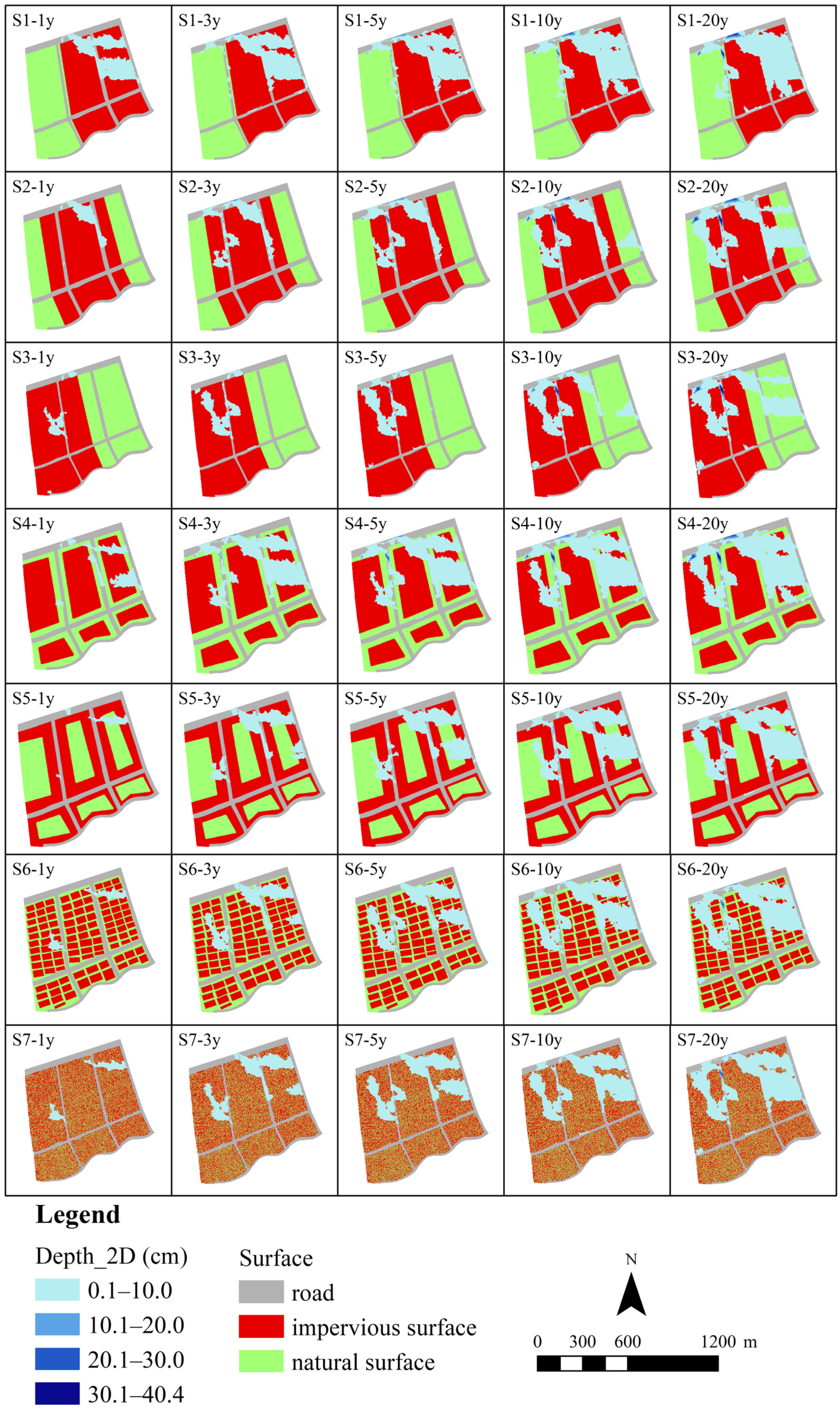
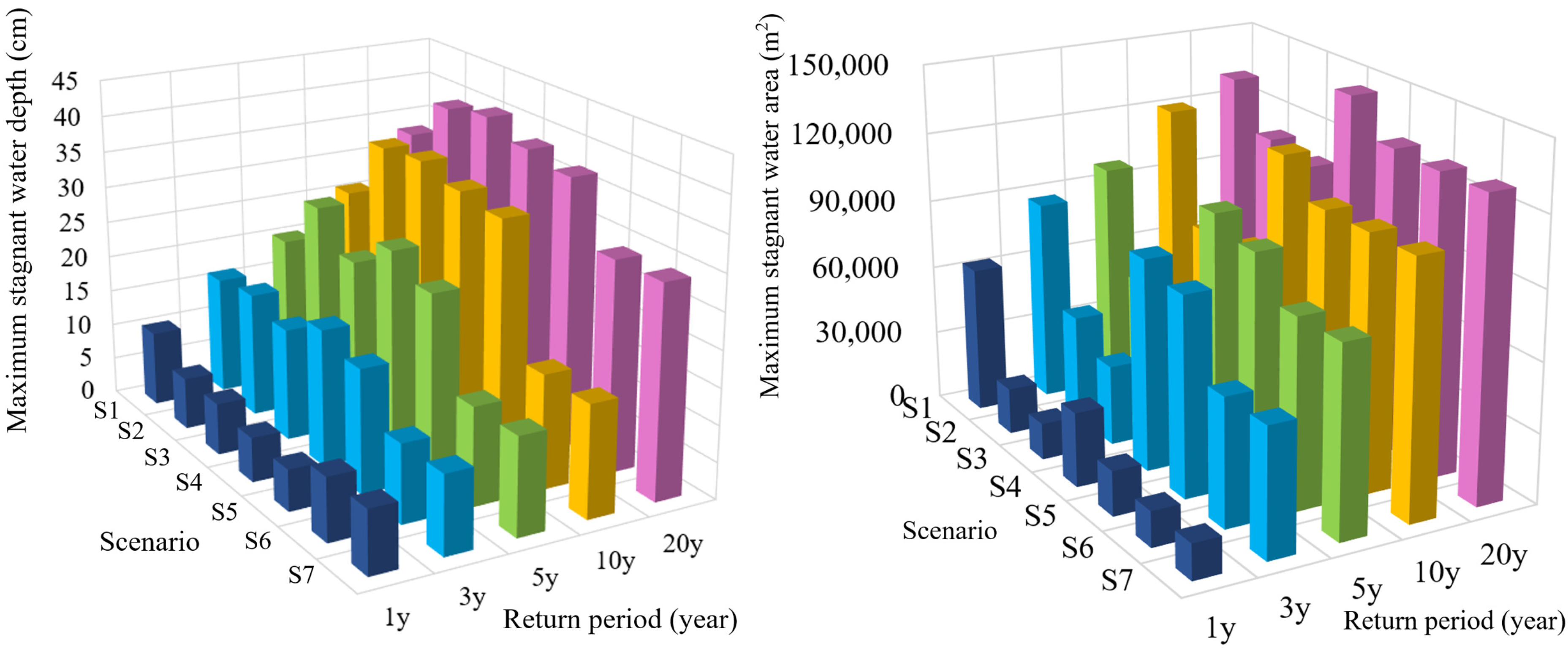
Figure 8 illustrates the waterlogging conditions under different scenarios; Table 4 and Figure 9 show detailed information of these conditions. In general, within the same impervious surface ratio, the maximum stagnant water depth increases with the increase in rainfall return period. The minimum value was 5.7 cm, occurring in S5 during the 1-year return period. The maximum was 40.4 cm, occurring in S3 during the 20-year return period. In the first set, the growth rate of stagnant water depth was the slowest in S1, increasing by 22.8 cm, and the fastest in S3, increasing by 33.3 cm. The stagnant water depths in the three scenarios differed significantly across rainfall return periods. For instance, in the 5-year return period, the stagnant water depth in S2 exceeded that in S3, while in the 10-year return period, S3 surpassed both S1 and S2. In the second set, S4 and S5 showed similar stagnant water depths, the difference between two scenarios ranging between 0.4 cm and 2.7 cm, with comparable growth rates. S4 increased by 32.3 cm, while S5 increased by 31.5 cm. In the third set, the stagnant water depths of the two scenarios were close, with differences ranging between 0 cm and 0.3 cm. S6 increased by 20.4 cm, and S7 increased by 20.5 cm.
Regarding the maximum stagnant water area, it ranged from 15,303.08 m2 to 145,389.95 m2. The minimum occurred in S6 and S7 during the 1-year return period, and the maximum occurred in S4 during the 20-year return period. In the first set, S3 had the smallest stagnant water area across almost every return period except for the 10-year one, ranging from 15,741.54 m2 to 107,019.20 m2. As the return period increased, the difference in stagnant water depth between S1 and S2 and that between S1 and S3 gradually decreased. The difference between S1 and S2 reduced from 46,759.43 m2 to 19,898.99 m2, and the difference between S1 and S3 reduced from 53,842.02 m2 to 24,036.18 m2. The difference between S2 and S3 was close across all the return periods. In the second set, the difference in the stagnant water area between S4 and S5 had no fixed trend. In the 3-year return period, the difference between the two scenarios was minimal, at 4986.14 m2. After that, the difference increased, the maximum was 14,668.71m2. In the third set, the two scenarios have similar stagnant water areas, with differences ranging from 0 to 162.01 m2. Overall, in the first set, S3 performed optimally with the smallest values in stagnant water area. In the second group, S5 exhibited relatively small stagnant water depth and area. In the third set, there was no significant difference in stagnant water depth and area values between the two scenarios.

3.3. Impervious Surface Optimization Plan Design

Figure 10 shows the spatial patterns of waterlogging under different optimization plans, and Table 5 adds detailed information about these patterns. In general, stagnant water depth and area of different impervious surface optimization plans increased with an increase in the return period. Regarding stagnant water depth, the minimum value occurred in P3 during the 1-year return period at 7.0 cm, while the maximum value occurred in P1 during the 20-year return period at 39.6 cm. The increase in stagnant water depth varied among all the optimization plans, with P5 having the slowest growth at 28 cm and P2 having the fastest at 32.4 cm. The stagnant water depths of the optimization plans were less than those of P1 after the 10-year return period. As for stagnant water area, the minimum value occurred in P2 during the 1-year return period, at 32,217.19 m2, while the maximum value of 142,068.38 m2 occurred in P1 during the 20-year return period. In all rainfall return periods, P2 and P3 consistently had smaller stagnant water areas than P1. P4 had a greater stagnant water area than P1 only in the 1-year return period, and the stagnant water areas of the rest were all smaller than that of the benchmark plan.

4. Discussion

4.1. Urban Waterlogging Characteristics with Different Impervious Surfaces Ratios

From 2010 to 2022, with the urbanization of the study area, the impervious surfaces in the study area showed an obviously upward trend. This process can be divided into four stages: the period of rapid development from 2010 to 2014, the stable period from 2014 to 2017, the recession period from 2017 to 2018, and the rapid growth period from 2018 to 2022. The first period from 2010 to 2014 was the construction stage of the Cultural and Sports Convention and Exhibition Center in Lin’an City. In the early days, the impervious surfaces were mainly concentrated in the southwest. After that, the impervious surfaces continued to grow. That was mainly because of the construction of stadiums and the rapid construction of surrounding roads. In the second period (2014–2017), the impervious surfaces in the study area were stable with a slight increase. The increase was mainly due to the improvement in the internal area of the Cultural and Sports Convention and Exhibition Center. Another reason was the construction of Yunjin Road and Wenjing Road. In the third period (2017–2018), impervious surfaces decreased. The main reason for this was that the residential area in the southwest of the study area had been demolished. Due to construction, half of the roads to the east of Jiuzhou Street have changed into natural surfaces. In the fourth period (2018–2022), the impervious surfaces continued to increase rapidly. It was mainly a result from the completion of the main roads and the construction of the community in the eastern region, as well as the improvements made to the surroundings of the Cultural and Sports Convention and Exhibition Center. With urban development, the stagnant water depth and area increased at the same time. There was a strong positive correlation between urban waterlogging and impervious surfaces. From the development of impervious surfaces in the study area over the past 12 years, the spatial distribution and changes of impervious surfaces have been greatly affected by the policy. This makes policy drivers an important contributor to the recent growth of impervious surfaces in urban areas [56,57].

4.2. Urban Waterlogging Characteristics under Different Spatial Distributions of Impervious Surfaces

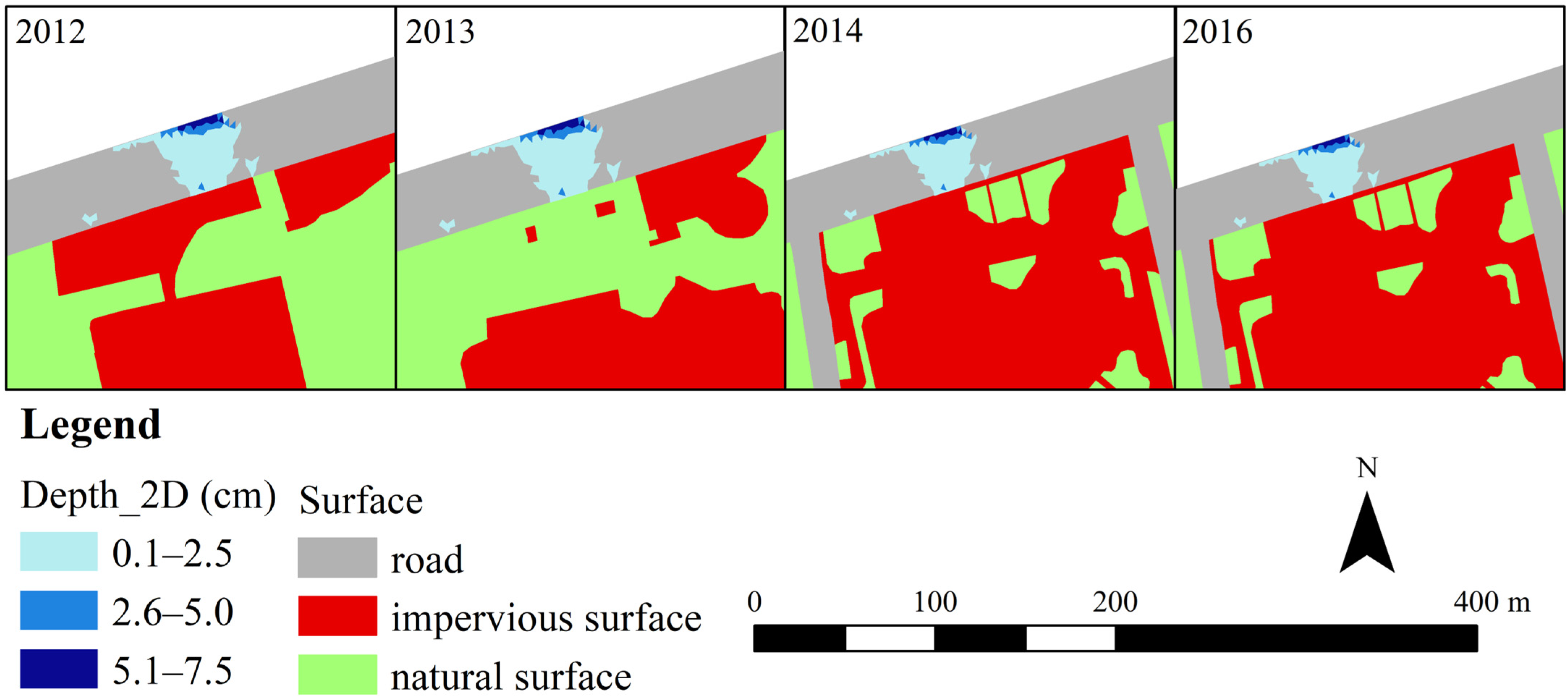
In general, the increase in impervious surfaces leads to greater stagnant water depth and area [44,45]. However, when comparing the stagnant water depth and area in the same return period in particular years, there is a contradictory relationship observed [58]. In a few years, the increase in impervious surfaces was negatively correlated with stagnant water depth and area. For example, impervious surfaces increased by 10,703 m2 in 2013 compared with 2012 in the study area. However, during the 1-year return period, the stagnant water depth and area were lower than those observed in 2012. A similar situation occurred during the 1-year, 10-year, and 20-year return periods in 2014 and 2016. The main reason for this was the spatial distribution of the impervious surfaces. In the year with more natural surfaces near the waterlogging point, rainwater had infiltrated more. The surface runoff and overflow were also reduced, and the overflow rainwater spread to both ends. In this context, not only did the proportion of impervious surfaces have an impact on urban waterlogging but also their spatial distribution. Even with the same impervious surface area, different distributions can lead to different urban waterlogging conditions.
Figure 11 shows the simulation results of the two sets during the 1-year return period. The stagnant water area during the 1-year return period in 2012, 2013, 2014, and 2016 was concentrated in the northern part of the study area. This is because the diameter of the pipe in the area was smaller at only 200 mm, and this made it easy for the pipe to overflow under overloading. The results shows that stagnant water first occurred on the roads with a high proportion of impervious surfaces. The main reason for this was that most of the pipes on these roads were between 200 mm and 300 mm in diameter. Only 17.03% of the pipes’ diameters were larger than 800 mm. Therefore, when a large amount of runoff occurred, the pipeline could not discharge in a short time, thus resulting in node overflow and stagnant water. In the first set (S1–S3), compared with the middle and lower reaches, the upper reaches had narrower pipeline diameters. Most pipelines on Yunjin Road had narrower diameters compared to Shuangyong Road. As a result, S1 had the largest stagnant water area among all the return periods. In the second set (S4 and S5), the stagnant water depth and area in S5 were smaller than those in S4. This was mainly affected the infiltration capacity of natural surfaces. Compared with S5, the natural surface of S4 cannot fully absorb runoff, leading to the increase in runoff. In the third set (S6 and S7), there was little difference in stagnant water depth and area between S6 and S7. The main reason for this was that more scattered natural surface patches can promote the formation, collection, and storage of rainwater [59,60].

4.3. Optimization Plans and Suggestions

The stagnant water area of various impervious surface optimization plans was similar to that of the benchmark plan (Figure 10), especially in low-lying areas. This was mainly because P2–P5 were minor modifications to the benchmark plan. According to the results (Table 5), although P3 was very effective in reducing stagnant water depth and area, it only considered the distribution of impervious surfaces. There were too many impervious surfaces along the roads, leaving large amounts of natural surfaces in the middle area. This kind of land use planning is unreasonable in practice. In actual deployment, impervious surfaces are usually located far away from roads. Due to the huge economic cost, it is almost impossible to build a new road system or completely change road distribution. Optimization should match the concept of urban renewal rather than urban reconstruction [59]. In contrast, P5 was a plan considering many factors. The spatial distribution of impervious surfaces in P5 was easier to realize than that of other plans. To sum up, it is suggested that impervious surfaces are distributed upstream and along the road. In addition, it is recommended that the aggregation of impervious surfaces is reduced as much as possible. In addition, it is suggested that the diameter of some pipelines on two roads in the eastern region is increased. Finally, it is recommended that low-lying areas such as roads in the north and middle of the study area are landfilled to reduce runoff.

4.4. Limitations and Future Perspectives

Three limitations need to be addressed for better understanding of the results: (1) When designing the spatial distribution scenarios of impervious surfaces, only three influencing factors (flow direction, pipe network distribution, and landscape pattern) were considered. In future research, other factors such as the overall patch size and the symmetry of impervious surfaces can be considered. With these extra factors, more spatial distribution scenarios can be designed to further explore the impact of impervious surfaces on urban waterlogging. (2) Changes in both impervious surfaces and drainage facilities can affect urban waterlogging. However, it is difficult to obtain long-timeseries drainage facilities data because data collection needs tremendous manual work and is usually organized by local governments. In addition, according to local knowledge, drainage facilities in the study area in the 2010–2022 period was relatively stable. In this context, changes in drainage facilities were not explored and may affect the accuracy of the results. (3) Due to the lack of pipe network, topography, historical rainfall, and stagnant water data of other cities, the conclusions drawn from optimizing the spatial distribution of impervious surfaces are only applicable to the study area. However, its research methods can be used for reference to similar areas. Future efforts can be made to collect data from other cities for comparative studies. With more cases, it is possible to obtain general conclusions in order to provide summarized recommendations for more cities.

5. Conclusions

This study established the urban waterlogging model of Lin’an City based on InfoWorks ICM. The model simulated the urban inundation parameters of the study area under different rainfall return periods and different impervious surface distributions. We investigated the influence of impervious surface spatial distribution changes on hydrological processes from the formation mechanism of waterlogging. We also quantitatively analyzed the influence of impervious surfaces spatial pattern on urban waterlogging. The main conclusions are as follows:
(1) The results showed that the distribution of impervious surfaces upstream and along roads, as well as increasing fragmentation, can effectively alleviate urban waterlogging. The phenomenon came from the fact that impervious surfaces along roads increased rainwater absorption, larger pipe diameters increased the flow within the pipes, and increased fragmentation of impervious surfaces enhanced rainwater infiltration.
(2) The results indicated that the P5 had good performance in reducing stagnant water depth and area. The main reason for this was that P5 integrated the advantages of P2–P4 and increased the area of impervious surfaces distributed upstream and along roads, which were beneficial to the absorption and infiltration of rainwater. The results revealed the potential of adjusting landscape configurations of impervious surfaces to control urban waterlogging. This study quantitatively analyzed the influence of spatial changes in impervious surfaces on urban waterlogging from two aspects: the change in the proportion of impervious surfaces and the change in impervious surface spatial distribution. Combined with the results of urban waterlogging process parameters and the optimization plans designed for the study area, suggestions were provided for reducing the impact of urban waterlogging and improving the safety and well-being of residents.

Author Contributions

Conceptualization, J.L. and T.H.; methodology, J.L.; software, J.L.; validation, J.L. and R.H.; formal analysis, J.L.; investigation, J.L. and H.H.; resources, J.L.; data curation, J.L. and Y.Z.; writing—original draft preparation, J.L. and H.H.; writing—review and editing, J.L., H.H., and T.H.; visualization, J.L. and R.H.; supervision, H.H., Y.Z., and T.H.; project administration, Y.Z. and T.H.; funding acquisition, Y.Z. and T.H. All authors have read and agreed to the published version of the manuscript.

Funding

This research was funded by Key R&D Program Projects in Zhejiang Province, grant number 2022C03107.

Data Availability Statement

For inquiries about the research data, please contact the corresponding author.

Acknowledgments

We thank the reviewers for their valuable feedback on this paper.

Conflicts of Interest

The authors declare no conflicts of interest.

References

  1. Hermanns, T.; Li, Q. Sustainability Impact Assessment of Land Use Changes in the Anthropocene. In The Anthropocene Debate and Political Science; Routledge: London, UK, 2018; ISBN 978-1-351-17412-1. [Google Scholar]
  2. El Kasri, J.; Lahmili, A.; Soussi, H.; Jaouda, I.; Bentaher, M. Trend Analysis of Meteorological Variables: Rainfall and Temperature. Civ. Eng. J. 2021, 7, 1868–1879. [Google Scholar] [CrossRef]
  3. Broekx, S.; Smets, S.; Liekens, I.; Bulckaen, D.; De Nocker, L. Designing a Long-Term Flood Risk Management Plan for the Scheldt Estuary Using a Risk-Based Approach. Nat. Hazards 2011, 57, 245–266. [Google Scholar] [CrossRef]
  4. Garcia, E.S.; Loáiciga, H.A. Sea-Level Rise and Flooding in Coastal Riverine Flood Plains. Hydrol. Sci. J. 2014, 59, 204–220. [Google Scholar] [CrossRef]
  5. Güneralp, B.; Güneralp, İ.; Liu, Y. Changing Global Patterns of Urban Exposure to Flood and Drought Hazards. Glob. Environ. Change 2015, 31, 217–225. [Google Scholar] [CrossRef]
  6. Smit, W. Urbanization in the Global South. In Oxford Research Encyclopedia of Global Public Health; Oxford University Press: Oxford, UK, 2021; ISBN 978-0-19-063236-6. [Google Scholar]
  7. Gu, C. Urbanization: Processes and Driving Forces. Sci. China Earth Sci. 2019, 62, 1351–1360. [Google Scholar] [CrossRef]
  8. Bai, X.; Shi, P.; Liu, Y. Society: Realizing China’s Urban Dream. Nature 2014, 509, 158–160. [Google Scholar] [CrossRef]
  9. Pan, Y.; Teng, T.; Wang, S.; Wang, T. Impact and Mechanism of Urbanization on Urban Green Development in the Yangtze River Economic Belt. Ecol. Indic. 2024, 158, 111612. [Google Scholar] [CrossRef]
  10. McCarthy, M.P.; Best, M.J.; Betts, R.A. Climate Change in Cities Due to Global Warming and Urban Effects. Geophys. Res. Lett. 2010, 37, 2010GL042845. [Google Scholar] [CrossRef]
  11. Moazzam, M.F.U.; Rahman, G.; Munawar, S.; Tariq, A.; Safdar, Q.; Lee, B.-G. Trends of Rainfall Variability and Drought Monitoring Using Standardized Precipitation Index in a Scarcely Gauged Basin of Northern Pakistan. Water 2022, 14, 1132. [Google Scholar] [CrossRef]
  12. Wang, C.; Geng, L.; Rodríguez-Casallas, J.D. How and When Higher Climate Change Risk Perception Promotes Less Climate Change Inaction. J. Clean. Prod. 2021, 321, 128952. [Google Scholar] [CrossRef]
  13. Campagnolo, L.; De Cian, E. Distributional Consequences of Climate Change Impacts on Residential Energy Demand across Italian Households. Energy Econ. 2022, 110, 106020. [Google Scholar] [CrossRef]
  14. Min, S.-K.; Zhang, X.; Zwiers, F.W.; Hegerl, G.C. Human Contribution to More-Intense Precipitation Extremes. Nature 2011, 470, 378–381. [Google Scholar] [CrossRef] [PubMed]
  15. Rohith, A.N.; Sudheer, K.P. A Novel Safe-Fail Framework for the Design of Urban Stormwater Drainage Infrastructures with Minimal Failure and Flood Severity. J. Hydrol. 2023, 627, 130393. [Google Scholar] [CrossRef]
  16. Liang, X.-Z. Extreme Rainfall Slows the Global Economy. Nature 2022, 601, 193–194. [Google Scholar] [CrossRef] [PubMed]
  17. Chen, J.; Li, Y.; Zhang, C.; Tian, Y.; Guo, Z. Urban Flooding Prediction Method Based on the Combination of LSTM Neural Network and Numerical Model. Int. J. Environ. Res. Public Health 2023, 20, 1043. [Google Scholar] [CrossRef]
  18. Zhang, Q.; Wu, Z.; Guo, G.; Zhang, H.; Tarolli, P. Explicit the Urban Waterlogging Spatial Variation and Its Driving Factors: The Stepwise Cluster Analysis Model and Hierarchical Partitioning Analysis Approach. Sci. Total Environ. 2021, 763, 143041. [Google Scholar] [CrossRef]
  19. Cheng, T.; Xu, Z.; Hong, S.; Song, S. Flood Risk Zoning by Using 2D Hydrodynamic Modeling: A Case Study in Jinan City. Math. Probl. Eng. 2017, 2017, e5659197. [Google Scholar] [CrossRef]
  20. Huang, H.; Lei, X.; Liao, W.; Zuo, X.; Wang, H. A Novel Multi-Strategy Hydrological Feature Extraction (MHFE) Method to Improve Urban Waterlogging Risk Prediction, a Case Study of Fuzhou City in China. Sci. Total Environ. 2023, 904, 165834. [Google Scholar] [CrossRef]
  21. Ma, B.; Wu, Z.; Hu, C.; Wang, H.; Xu, H.; Yan, D. Process-Oriented SWMM Real-Time Correction and Urban Flood Dynamic Simulation. J. Hydrol. 2022, 605, 127269. [Google Scholar] [CrossRef]
  22. Mei, C.; Liu, J.; Wang, H.; Li, Z.; Yang, Z.; Shao, W.; Ding, X.; Weng, B.; Yu, Y.; Yan, D. Urban Flood Inundation and Damage Assessment Based on Numerical Simulations of Design Rainstorms with Different Characteristics. Sci. China E Technol. Sci. 2020, 63, 2292–2304. [Google Scholar] [CrossRef]
  23. Hsu, M.H.; Chen, S.H.; Chang, T.J. Inundation Simulation for Urban Drainage Basin with Storm Sewer System. J. Hydrol. 2000, 234, 21–37. [Google Scholar] [CrossRef]
  24. Zhang, B.; Chen, M.; Ma, Z.; Zhang, Z.; Yue, S.; Xiao, D.; Zhu, Z.; Wen, Y.; Lü, G. An Online Participatory System for SWMM-Based Flood Modeling and Simulation. Environ. Sci. Pollut. Res. 2022, 29, 7322–7343. [Google Scholar] [CrossRef] [PubMed]
  25. Fadhel, S.; Rico-Ramirez, M.A.; Han, D. Sensitivity of Peak Flow to the Change of Rainfall Temporal Pattern Due to Warmer Climate. J. Hydrol. 2018, 560, 546–559. [Google Scholar] [CrossRef]
  26. Xu, T.; Xie, Z.; Jiang, F.; Yang, S.; Deng, Z.; Zhao, L.; Wen, G.; Du, Q. Urban Flooding Resilience Evaluation with Coupled Rainfall and Flooding Models: A Small Area in Kunming City, China as an Example. Water Sci. Technol. 2023, 87, 2820–2839. [Google Scholar] [CrossRef] [PubMed]
  27. Cao, Q.; Cao, J.; Xu, R. Optimizing Low Impact Development for Stormwater Runoff Treatment: A Case Study in Yixing, China. Water 2023, 15, 989. [Google Scholar] [CrossRef]
  28. Lin, J.; Zhu, H.; Liu, G.; Huang, M.; Xie, Z. Composite Scheme of Comprehensive Improvement for Urban Rivers. IOP Conf. Ser. Earth Environ. Sci. 2020, 546, 032005. [Google Scholar] [CrossRef]
  29. Chen, J.; Chang, K.; Karacsonyi, D.; Zhang, X. Comparing Urban Land Expansion and Its Driving Factors in Shenzhen and Dongguan, China. Habitat. Int. 2014, 43, 61–71. [Google Scholar] [CrossRef]
  30. Xu, T.; Xie, Z.; Zhao, F.; Li, Y.; Yang, S.; Zhang, Y.; Yin, S.; Chen, S.; Li, X.; Zhao, S.; et al. Permeability Control and Flood Risk Assessment of Urban Underlying Surface: A Case Study of Runcheng South Area, Kunming. Nat. Hazards 2022, 111, 661–686. [Google Scholar] [CrossRef]
  31. Zhang, Q.; Wu, Z.; Tarolli, P. Investigating the Role of Green Infrastructure on Urban WaterLogging: Evidence from Metropolitan Coastal Cities. Remote Sens. 2021, 13, 2341. [Google Scholar] [CrossRef]
  32. Basnet, K.; Chettri, K.; Parajuli, G.; Bhandari, A. Hydrological and Hydraulic Analyses of Urban Storm Water Drainage System of Major Area of Pokhara, Nepal. J. Innov. Eng. Educ. 2020, 3, 78–91. [Google Scholar] [CrossRef]
  33. Jiang, W.; Yu, J. Impact of Rainstorm Patterns on the Urban Flood Process Superimposed by Flash Floods and Urban Waterlogging Based on a Coupled Hydrologic–Hydraulic Model: A Case Study in a Coastal Mountainous River Basin within Southeastern China. Nat. Hazards 2022, 112, 301–326. [Google Scholar] [CrossRef]
  34. Deb, D.; Schneider, P.; Dudayev, Z.; Emon, A.; Areng, S.S.; Mozumder, M.M.H. Perceptions of Urban Pollution of River Dependent Rural Communities and Their Impact: A Case Study in Bangladesh. Sustainability 2021, 13, 13959. [Google Scholar] [CrossRef]
  35. Ning, Y.-F.; Zhang, J.-T.; Huang, J.-H.; Long, H.-F.; Huang, Q.-S. Systematic Treatment of Urban River Pollution. IOP Conf. Ser. Earth Environ. Sci. 2020, 446, 032021. [Google Scholar] [CrossRef]
  36. Chen, X.; Wang, Y.; Jiang, L.; Huang, X.; Huang, D.; Dai, W.; Cai, Z.; Wang, D. Water Quality Status Response to Multiple Anthropogenic Activities in Urban River. Environ. Sci. Pollut. Res. 2023, 30, 3440–3452. [Google Scholar] [CrossRef]
  37. Ministry of Water Resources. Statistical Bulletin of Flood and Drought Disasters in China. Available online: http://www.mwr.gov.cn/sj/tjgb/zgshzhgb/ (accessed on 6 April 2024).
  38. Lin’an District Bureau of Statistics. Statistical Bulletin of National Economic and Social Development in Lin’an District of Hangzhou City in 2022. Available online: https://www.linan.gov.cn/art/2023/4/6/art_1229252926_4155359.html?eqid=85e8e9d800006c6a000000046435ac40 (accessed on 6 April 2024).
  39. Liao, D.; Zhu, H.; Zhou, J.; Wang, Y.; Sun, J. Study of the Natural Rainstorm Moving Regularity Method for Hyetograph Design. Theor. Appl. Climatol. 2019, 138, 1311–1321. [Google Scholar] [CrossRef]
  40. Keifer, C.J.; Chu, H.H. Synthetic Storm Pattern for Drainage Design. J. Hydraul. Div. 1957, 83, 1332-1–1332-25. [Google Scholar] [CrossRef]
  41. Chen, J.; Li, Y.; Zhang, C. The Effect of Design Rainfall Patterns on Urban Flooding Based on the Chicago Method. Int. J. Environ. Res. Public Health 2023, 20, 4245. [Google Scholar] [CrossRef]
  42. Silveira, A.L.L.d. Cumulative Equations for Continuous Time Chicago Hyetograph Method. RBRH 2016, 21, 646–651. [Google Scholar] [CrossRef]
  43. Pan, C.; Wang, X.; Liu, L.; Huang, H.; Wang, D. Improvement to the Huff Curve for Design Storms and Urban Flooding Simulations in Guangzhou, China. Water 2017, 9, 411. [Google Scholar] [CrossRef]
  44. Krvavica, N.; Rubinić, J. Evaluation of Design Storms and Critical Rainfall Durations for Flood Prediction in Partially Urbanized Catchments. Water 2020, 12, 2044. [Google Scholar] [CrossRef]
  45. Gong, Y.; Li, X.; Zhai, D.; Yin, D.; Song, R.; Li, J.; Fang, X.; Yuan, D. Influence of Rainfall, Model Parameters and Routing Methods on Stormwater Modelling. Water Resour. Manag. 2018, 32, 735–750. [Google Scholar] [CrossRef]
  46. Peng, H.-Q.; Liu, Y.; Gao, X.-L.; Wang, H.-W.; Chen, Y.; Cai, H.-Y. Calculation of Intercepted Runoff Depth Based on Stormwater Quality and Environmental Capacity of Receiving Waters for Initial Stormwater Pollution Management. Environ. Sci. Pollut. Res. 2017, 24, 24681–24689. [Google Scholar] [CrossRef] [PubMed]
  47. Yang, Y.; Ng, S.T.; Dao, J.; Zhou, S.; Xu, F.J.; Xu, X.; Zhou, Z. BIM-GIS-DCEs Enabled Vulnerability Assessment of Interdependent Infrastructures—A Case of Stormwater Drainage-Building-Road Transport Nexus in Urban Flooding. Autom. Constr. 2021, 125, 103626. [Google Scholar] [CrossRef]
  48. Wang, L.; Li, Y.; Hou, H.; Chen, Y.; Fan, J.; Wang, P.; Hu, T. Analyzing Spatial Variance of Urban Waterlogging Disaster at Multiple Scales Based on a Hydrological and Hydrodynamic Model. Nat. Hazards 2022, 114, 1915–1938. [Google Scholar] [CrossRef]
  49. Wei, H.; Zhang, L.; Liu, J. Hydrodynamic Modelling and Flood Risk Analysis of Urban Catchments under Multiple Scenarios: A Case Study of Dongfeng Canal District, Zhengzhou. Int. J. Environ. Res. Public Health 2022, 19, 14630. [Google Scholar] [CrossRef] [PubMed]
  50. Sidek, L.M.; Jaafar, A.S.; Majid, W.H.A.W.A.; Basri, H.; Marufuzzaman, M.; Fared, M.M.; Moon, W.C. High-Resolution Hydrological-Hydraulic Modeling of Urban Floods Using InfoWorks ICM. Sustainability 2021, 13, 10259. [Google Scholar] [CrossRef]
  51. Çirağ, B.; Firat, M. Two-Dimensional (2D) Flood Analysis and Calibration of Stormwater Drainage Systems Using Geographic Information Systems. Water Sci. Technol. 2023, 87, 2577–2596. [Google Scholar] [CrossRef] [PubMed]
  52. Yang, B.; Lee, D. Urban Green Space Arrangement for an Optimal Landscape Planning Strategy for Runoff Reduction. Land 2021, 10, 897. [Google Scholar] [CrossRef]
  53. Mei, C.; Shi, H.; Liu, J.; Song, T.; Wang, J.; Gao, X.; Wang, H.; Li, M. Analyzing Urban Form Influence on Pluvial Flooding via Numerical Experiments Using Random Slices of Actual City Data. J. Hydrol. 2024, 633, 130916. [Google Scholar] [CrossRef]
  54. Li, H.; Wang, Q.; Li, M.; Zang, X.; Wang, Y. Identification of Urban Waterlogging Indicators and Risk Assessment Based on MaxEnt Model: A Case Study of Tianjin Downtown. Ecol. Indic. 2024, 158, 111354. [Google Scholar] [CrossRef]
  55. Liu, W.; Zhang, X.; Feng, Q.; Yu, T.; Engel, B.A. Analyzing the Impacts of Topographic Factors and Land Cover Characteristics on Waterlogging Events in Urban Functional Zones. Sci. Total Environ. 2023, 904, 166669. [Google Scholar] [CrossRef]
  56. Yu, H.; Zhao, Y.; Fu, Y.; Li, L. Spatiotemporal Variance Assessment of Urban Rainstorm Waterlogging Affected by Impervious Surface Expansion: A Case Study of Guangzhou, China. Sustainability 2018, 10, 3761. [Google Scholar] [CrossRef]
  57. Lu, D.; Song, K.; Zang, S.; Jia, M.; Du, J.; Ren, C. The Effect of Urban Expansion on Urban Surface Temperature in Shenyang, China: An Analysis with Landsat Imagery. Environ. Model. Assess. 2015, 20, 197–210. [Google Scholar] [CrossRef]
  58. Lin, J.; Zhang, W.; Wen, Y.; Qiu, S. Evaluating the Association between Morphological Characteristics of Urban Land and Pluvial Floods Using Machine Learning Methods. Sustain. Cities Soc. 2023, 99, 104891. [Google Scholar] [CrossRef]
  59. Lin, J.; He, P.; Yang, L.; He, X.; Lu, S.; Liu, D. Predicting Future Urban Waterlogging-Prone Areas by Coupling the Maximum Entropy and FLUS Model. Sustain. Cities Soc. 2022, 80, 103812. [Google Scholar] [CrossRef]
  60. Yu, H.; Zhao, Y.; Fu, Y. Optimization of Impervious Surface Space Layout for Prevention of Urban Rainstorm Waterlogging: A Case Study of Guangzhou, China. J. Environ. Res. Public Health 2019, 16, 3613. [Google Scholar] [CrossRef]
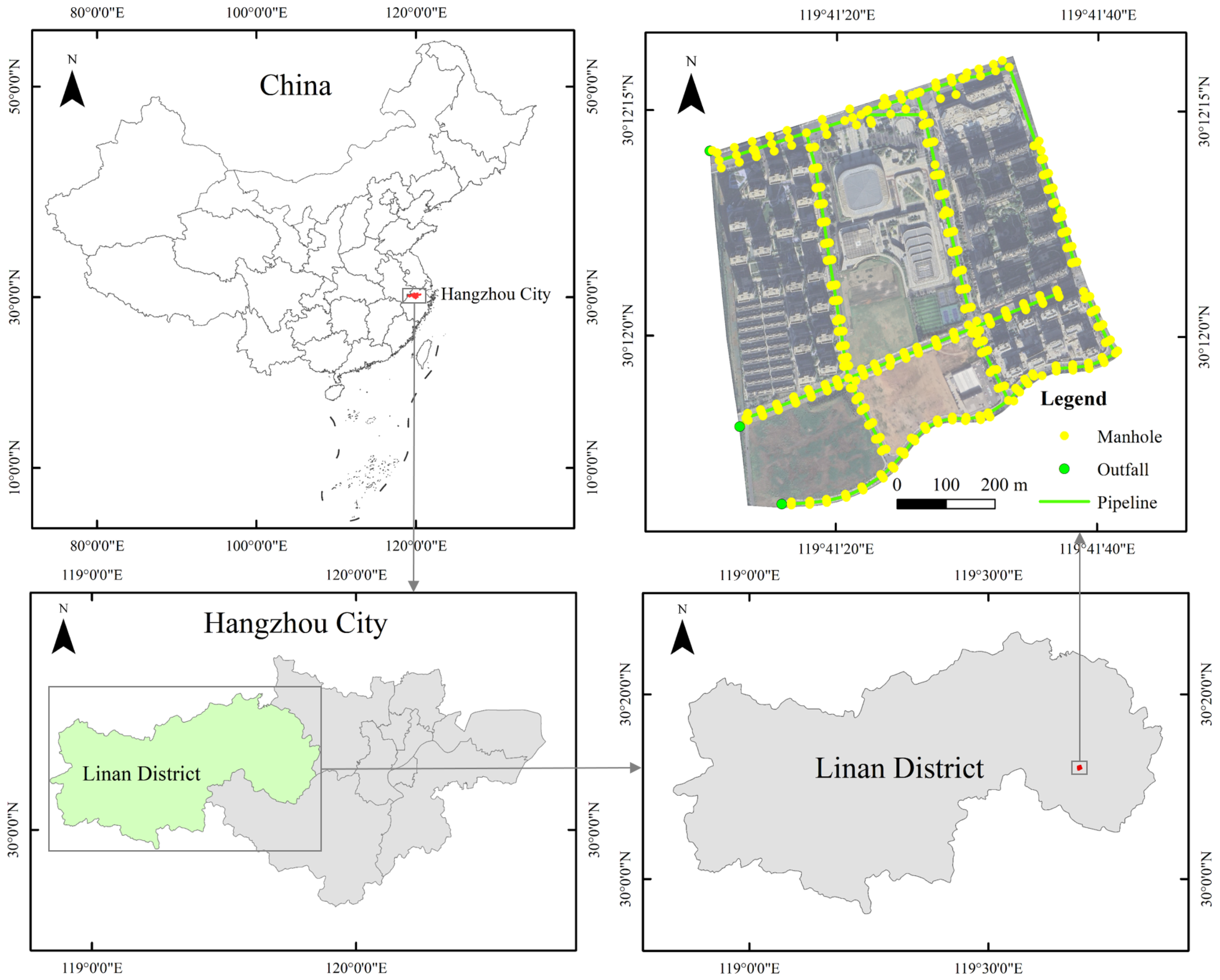
Figure 1. Overview of the study area.
Remotesensing 16 02130 g001
Figure 2. Hyetograph of the designed rainfall events.
Remotesensing 16 02130 g002
Figure 3. Overall workflow for this study.
Remotesensing 16 02130 g003
Figure 4. Impervious surface spatial distribution scenarios: (S1) impervious surface upstream; (S2) impervious surface middle stream; (S3) impervious surface downstream; (S4) impervious surface away from the roads; (S5) impervious surface along the roads; (S6) impervious surface with uniform distribution; and (S7) impervious surface with random distribution.
Remotesensing 16 02130 g004
Figure 5. Design of optimization plans: (P1) Land use in 2022; (P2) Impervious surface concentrated upstream; (P3) Impervious surface distributed along roads; (P4) Increase the fragmentation of impervious surfaces; and (P5) Comprehensive distribution.
Remotesensing 16 02130 g005
Figure 6. Distribution of impervious surface area changes in the study area from 2010 to 2022.
Remotesensing 16 02130 g006
Figure 7. Maximum stagnant water depth and area in the study area from 2010 to 2022 under different rainfall return periods.
Remotesensing 16 02130 g007
Figure 8. Simulation results of different scenarios under different return periods: (S1) impervious surface upstream; (S2) impervious surface middle stream; (S3) impervious surface downstream; (S4) impervious surface away from the roads; (S5) impervious surface along the roads; (S6) impervious surface with uniform distribution; and (S7) impervious surface with random distribution.
Remotesensing 16 02130 g008
Figure 9. Maximum stagnant water depth and area in the spatial distribution of impervious surfaces in different return periods.
Remotesensing 16 02130 g009
Figure 10. Simulation results of different optimization plans under different return periods: (P1) Land use in 2022; (P2) Impervious surface concentrated upstream; (P3) Impervious surface distributed along roads; (P4) Increase the fragmentation of impervious surfaces; and (P5) Comprehensive distribution.
Remotesensing 16 02130 g010
Figure 11. Comparison of stagnant water between different impervious surface distributions during the 1-year return period.
Remotesensing 16 02130 g011
Table 1. List of geographic data in the study area.
TypeResolution (m)DateData Source
DEM2-Surveying and Mapping Department of Lin’an
Rainfall data-31 July 2022National Meteorological Science Data Center “http://data.cma.cn/
(accessed on 30 May 2024)
13 September 2022
Pipeline network data--Urban Administration of Lin’an
Multi-temporal high-resolution remote sensing images0.2730 June 2010Google Earth
8 June 2011
20 September 2012
15 November 2013
16 December 2014
9 February 2016
18 May 2017
29 March 2018
16 October 2019
5 March 2020
19 January 2021
Aerial images0.2March 2022Aerial photography
Table 2. Parameters for three kinds of runoff-producing surfaces.
SurfaceRoutine ParameterSurface TypeRunoff ModelInitial Loss/mmFixed Runoff CoefficientInitial Infiltration Rate (mm/h)Stable Infiltration Rate (mm/h)Decay Rate Coefficient (1/h)
Road0.02ImperviousFixed1.50.9---
Impervious surface0.02ImperviousFixed1.50.85---
Natural surface0.035PerviousHorton2.8-7642
Table 3. Maximum stagnant water depth and area in the study area from 2010 to 2022 under different rainfall return periods.
YearMaximum Stagnant Water Depth in Each Return Period/cmStagnant Water Area in Each Return Period/m2
1 year3 years5 years10 years20 years1 year3 years5 years10 years20 years
201002.44.66.39.301392.644334.1514824.6148,403.20
201102.95.26.910.801369.441777.3233,973.5270,384.74
20126.38.710.312.518.61705.522624.064268.8355,145.4595,111.17
20134.27.18.211.719.11185.092633.4710,695.7262,557.18107,174.93
20147.510.211.417.127.61568.2916,808.3231,866.5674,803.97110,935.19
20167.310.913.216.627.21568.2914,110.1632,964.9675,010.02109,173.85
20177.711.314.816.624.01483.3514,513.3639,615.8671,905.11107,714.62
20181.611.615.716.022.61125.5018,145.5821,042.0758,920.5780,676.55
20194.513.718.720.327.02836.6220,980.5044,646.9982,133.2792,412.86
20207.013.914.419.130.62650.1424,643.0861,711.5891,511.86103,580.09
20217.013.418.127.333.321,078.5372,602.58107,832.98114,098.09130,042.46
20228.218.527.635.539.636,688.7396,311.57111,739.52128,098.60142,068.38
Table 4. Maximum stagnant water depth and area in the spatial distribution of impervious surfaces in different return periods.
ScenarioMaximum Stagnant Water Depth in Each Return Period/cmStagnant Water Area in Each Return Period/m2
1 year3 years5 years10 years20 years1 year3 years5 years10 years20 years
S110.316.320.325.933.163,162.1087,385.0598,403.94120,506.20131,055.38
S27.117.228.035.039.219,838.4745,883.2855,408.3873,746.77111,156.39
S37.115.523.235.740.415,741.5434,560.0344,561.4975,383.69107,019.20
S46.118.827.834.238.432,003.4491,172.91105,178.51124,910.79145,389.95
S55.717.025.133.337.219,333.7986,186.7798,191.78110,242.08130,735.65
S68.710.813.515.729.115,303.0855,183.6881,605.45110,060.51129,569.95
S78.710.813.415.429.215,303.0855,154.4281,638.16109,898.50129,616.97
Table 5. Maximum stagnant water depth and area in the optimization plans under different return periods.
PlanMaximum Stagnant Water Depth in Each Return Period/cmStagnant Water Area in Each Return Period/m2
1 year3 years5 years10 years20 years1 year3 years5 years10 years20 years
P18.218.527.635.539.636,688.7396,311.57111,739.52128,098.60142,068.38
P27.118.328.135.439.532,217.1990,575.56104,762.43123,353.35140,012.86
P37.015.122.832.937.832,918.3189,037.38103,430.89120,266.93136,420.80
P48.217.526.635.139.336,864.1995,800.20110,749.82126,898.30139,796.53
P58.918.426.132.936.936,577.8995,835.23110,619.33128,047.53137,729.71
Disclaimer/Publisher’s Note: The statements, opinions and data contained in all publications are solely those of the individual author(s) and contributor(s) and not of MDPI and/or the editor(s). MDPI and/or the editor(s) disclaim responsibility for any injury to people or property resulting from any ideas, methods, instructions or products referred to in the content.