Article

Predicting Winter Wheat Yield with Dual-Year Spectral Fusion, Bayesian Wisdom, and Cross-Environmental Validation

1
Institute of Farmland Irrigation, Chinese Academy of Agricultural Sciences, Xinxiang 453002, China
2
Xingtai Agricultural Science Research Institute, Xingtai 054000, China
3
Henan Institute of Water Resources Research, Zhengzhou 450003, China
4
Faculty of Physics and Electrical Engineering, Xinxiang University, Xinxiang 453000, China
*
Author to whom correspondence should be addressed.
Remote Sens. 2024, 16(12), 2098; https://doi.org/10.3390/rs16122098
Submission received: 8 May 2024 / Revised: 28 May 2024 / Accepted: 6 June 2024 / Published: 10 June 2024

Abstract

:
Winter wheat is an important grain that plays a crucial role in agricultural production and ensuring food security. Its yield directly impacts the stability and security of the global food supply. The accurate monitoring of grain yield is imperative for precise agricultural management. This study aimed to enhance winter wheat yield predictions with UAV remote sensing and investigate its predictive capability across diverse environments. In this study, RGB and multispectral (MS) data were collected on 6 May 2020 and 10 May 2022 during the grain filling stage of winter wheat. Using the Pearson correlation coefficient method, we identified 34 MS features strongly correlated with yield. Additionally, we identified 24 texture features constructed from three bands of RGB images and a plant height feature, making a total of 59 features. We used seven machine learning algorithms (Cubist, Gaussian process (GP), Gradient Boosting Machine (GBM), Generalized Linear Model (GLM), K-Nearest Neighbors algorithm (KNN), Support Vector Machine (SVM), Random Forest (RF)) and applied recursive feature elimination (RFE) to nine feature types. These included single-sensor features, fused sensor features, single-year data, and fused year data. This process yielded diverse feature combinations, leading to the creation of seven distinct yield prediction models. These individual machine learning models were then amalgamated to formulate a Bayesian Model Averaging (BMA) model. The findings revealed that the Cubist model, based on the 2020 and 2022 dataset, achieved the highest R2 at 0.715. Notably, models incorporating both RGB and MS features outperformed those relying solely on either RGB or MS features. The BMA model surpassed individual machine learning models, exhibiting the highest accuracy (R2 = 0.725, RMSE = 0.814 t·ha−1, MSE = 0.663 t·ha−1). Additionally, models were developed using one year’s data for training and another year’s data for validation. Cubist and GLM stood out among the seven individual models, delivering strong predictive performance. The BMA model, combining these models, achieved the highest R2 of 0.673. This highlights the BMA model’s ability to generalize for multi-year data prediction.

1. Introduction

Winter wheat, a critical global food crop, plays a pivotal role in both agricultural production and food security [1]. With the world’s population rapidly increasing and economic development on the rise, ensuring consistent yield growth for winter wheat has become an urgent agricultural imperative [2]. Consequently, accurate early yield prediction has become a paramount necessity for agricultural progress [2]. Traditional methods for gauging winter wheat yield predominantly hinge on destructive sampling, necessitating the harvesting, threshing, and weighing of sample areas. However, these methods require substantial human, material, and financial resources and do not provide accurate yield information before harvest [3].
Satellite remote sensing has made significant advancements in terms of spatial, temporal, and spectral resolution. However, it comes with limitations such as limited flexibility, high costs, cloud coverage constraints, and lack of automation, which have hindered its widespread adoption [4]. However, the emergence of UAVs has opened up new possibilities in remote sensing. These UAVs provide data with unprecedented spatial, spectral, and temporal resolution, facilitating rapid evolution in the field [5]. The use of images captured by UAVs has become a cost-effective alternative to expensive aircraft and satellite products. UAVs offer the advantage of carrying multiple sensors and are not constrained by issues like repeat cycles. They can undertake multiple missions throughout a crop’s entire growth cycle, capturing data with centimeter-level accuracy [6,7]. UAVs can be equipped with various sensors, including RGB (red-green-blue) sensors and multispectral (MS) sensors. RGB sensors are favored for their cost-effectiveness and high spatial resolution [8]. On the flip side, MS sensors offer excellent spectral resolution, with each sensor being sensitive within a specific spectral range. When using UAVs for crop phenotypic information, the red, near-red, and red-edge bands have proven to be effective [9,10,11]. An example study by Prey [12] used RGB and MS sensors to predict grain yield and demonstrated their effectiveness.
MS features offer valuable insights into estimating aboveground biomass and nitrogen content by enabling the derivation of multiple spectral indices from the five bands of MS data [13,14]. In addition to spectral indices, RGB images also contain texture features that are closely related to vegetation growth. These texture features capture spatial information about the distribution of vegetation and non-vegetation areas in the image and their interactions with the environment. They reflect the visual characteristics of homogeneous phenomena in the image [15]. For example, Yue et al. [16] discovered that integrating RGB spectral indices and image texture metrics at various spatial resolutions improved the R² value for estimating winter wheat biomass. The R² value increased to 0.84, compared to 0.76 when using spectral indices alone. Similarly, Zheng et al. [17] found that combining texture features with spectral indices in stepwise multiple linear regression improved model performance (R2 = 0.78). These findings have implications for research aiming to incorporate texture features as input variables in predictive models. To extract plant height (PH) information, a digital surface model (DSM) is typically subtracted from a digital terrain model (DTM) in RGB images. This process yields a canopy height model representing the height difference between the vegetation canopy and the ground, thus providing the plant height feature [18]. Cao et al. [19] demonstrated that integrating the extracted tree height feature into the mangrove classification process improved classification accuracy, underscoring the validity and usefulness of elevation information derived from DSM and DTM.
Machine learning models built based on spectral and structural features are widely used in the development of prediction systems, especially for complex systems with uncertainty [20]. Revill [21] used machine learning with Gaussian process regression to calibrate LAI UAV models using ground data. Barzin [22] used a machine learning approach to estimate the nitrogen (N) content of corn leaves based on UAV MS data and identified Gradient Lifter and Random Forest as the most suitable models for estimating leaf N. Proietti [23] introduced a generalized linear model for a time series that can integrate alternative spectral estimation methods within the same probability-based framework. Li [24] investigated an SVM method for field weed identification involving multiple features using spectral data from soil images. Silva et al. [25] found that the Cubist model is the best multivariate model for predicting sand and clay content from soil VIS-NIR-SWIR spectra. Cao et al. [26] estimated mangrove biomass using the K-Nearest Neighbors (KNN) method, and the results showed an improvement in accuracy with increasing scale. The effectiveness of these seven machine learning methods has been demonstrated in the studies mentioned above. Recursive feature selection as a data dimensionality reduction method can eliminate redundant information and noise interference. It can be applied to filter input features in various prediction models for phenotypic information, such as predicting chlorophyll content [27], predicting winter wheat yield [28], and estimating alpine grassland vegetation cover [29], among others.
Numerous studies have focused on using multi-year data to predict crop phenotypic information, showing promising predictive performance. Wang et al. [30] used four years of hyperspectral data to predict straight-chain starch content in rice. Their results showed that the inclusion of texture variables based on hyperspectral UAV imagery simplified data collection and improved estimation accuracy. Zheng et al. [31] combined two years of UAV MS data with soil hyperspectral data to estimate the nitrogen (N) concentration of rice plants and achieved improved prediction accuracy. Qiao et al. [32] used UAV MS data to estimate leaf area index (LAI) of maize in a two-year experiment conducted in 2021 and 2022. The study found that the depth feature-based LAI estimation model had the highest accuracy when applied to the two-year dataset. Although these studies used multi-year data to construct prediction models, there are currently few research works that use one-year data as a training set and one-year data as a validation set to build prediction models. This poses a challenge for future research in this area.
Furthermore, the non-linear and unsteady properties of UAV spectra make yield prediction difficult, especially when relying only on separate machine learning models. This is because using individual machine learning models to achieve optimal prediction performance does not take into account the structure of the model and parameter settings [33], resulting in uncertainty. Ensemble learning models provide a good way to reduce uncertainty in prediction by combining several good individual machine learning models [34]. Ensemble machine learning algorithms combine multiple weak models to create a stronger and more robust predictive model. Leveraging the strengths of diverse models, these algorithms enhance prediction accuracy and generalization. They have demonstrated impressive performance across various domains. BMA is an ensemble learning model. Unlike other ensemble learning methods, BMA not only gives deterministic weighted averages for the models but also creates prediction distributions to analyze uncertainties linked with deterministic predictions [35]. There are many reports showing that BMA methods can provide better performance than individual machine learning models [36,37]. However, it is less known whether BMA models will improve accuracy and reduce uncertainty in yield prediction.
The aim of this study is to build seven yield prediction models using UAV RGB and MS data from 2020 and 2022. The aim is to evaluate the generalizability and generalization ability of each model. The first step is to extract texture features and plant height features from the RGB data and spectral indices from the MS data. Then, the single- and multi-sensor features are verified using recursive feature elimination (RFE) methods with seven machine learning algorithms. Machine learning models are then created based on the verified features. Finally, one year’s data are used as the training set, while the other year’s data are used as the validation set. The performance of the machine learning models with satisfactory results is evaluated by predicting the yield.
The paper makes several important contributions, outlined below:
Introducing a novel model framework: Combining a RFE method with a machine learning model while combining the results of multiple individual machine learning models to build one ensemble model.
Building Yield Prediction Models: This study built seven yield prediction models using multi-year, multi-sensor data fusion. These models use one year’s data as a training set and another year’s data as a validation set.
Performance of the BMA ensemble model: The BMA ensemble model consistently demonstrated good prediction performance. Even when evaluating unknown datasets, the BMA ensemble model demonstrated a certain level of accuracy.

2. Materials and Methods

2.1. Experimental Area and Design

The experiment took place in the 2019–2020 and 2021–2022 growing seasons at the Chinese Academy of Agricultural Sciences Comprehensive Experimental Base in Xinxiang County, Xinxiang City, Henan Province (113°45′38″E, 35°8′10″N, Figure 1). This region is located in the northern part of Henan Province. The average annual rainfall and temperature are 573 mm and 15.8 °C, respectively.
A total of 180 test plots were established in the 2019–2020 growing season and were subjected to three different irrigation treatments throughout the fertility period: W1 (240 mm), W2 (190 mm), and W3 (145 mm). Each irrigation treatment consisted of 60 plots, and each plot had a row spacing of 20 cm, a length of 8 m, and a width of 1.4 m, resulting in an area of 11.2 m2 (Figure 1). Thirty wheat varieties suitable for cultivation in the Huanghuai wheat region were selected as test materials. To ensure the objectivity of the experiment, three replicates of each treatment were performed. The winter wheat was sown at the end of October 2019 and harvested on 3 June 2020. As in the 2019–2020 growing season, a total of 180 test plots were created in the 2021–2022 growing season. During the reproductive period, the wheat plants were subjected to six different irrigation treatments: W1 (300 mm), W2 (240 mm), W3 (180 mm), W4 (120 mm), W5 (60 mm), and W6 (0 mm). A total of 10 varieties of wheat commonly grown on the north China plain were used in the experiment. Each treatment consisted of 30 experimental plots, each 4 m long and 1.4 m wide. Adjacent plots were 0.4 m apart. The winter wheat was sown at the end of October 2021 and harvested on 5 June 2022. During the harvest for both growing seasons 2019–2020 and 2021–2022, wheat grain from each plot was collected separately using a plot combine. The harvested wheat from each plot was then placed in a numbered bag and dried in the laboratory to a constant mass. The winter wheat from each plot was then weighed and the yield was calculated based on the plot area.

2.2. UAV Spectral Data Acquisition

The MS data were collected using a DJI M210 drone manufactured by Shenzhen DJI Technology Co., Ltd., located in Shenzhen, China. The M210 was equipped with a Micasense RedEdgeMX MS camera. Additionally, the RGB data were captured using a DJI Phantom 4 Pro with an RGB sensor (Figure 2). The RedEdge MX sensor utilizes five bands of spectral imaging technology, including red, green, blue, near-infrared and red-edge. The red, green, and blue bands have center wavelengths of 668 nm, 560 nm, and 475 nm, respectively, while the near-infrared band has a center wavelength of 840 nm, and the red-edge band has a center wavelength of 717 nm. All channels have a resolution of 1280 × 960 and deliver high quality images with a wide 47.2° field of view. On the other hand, the DJI Phantom 4 Pro is equipped with a high-quality RGB sensor that can capture detailed, clear and crisp images. The sensor has a resolution of 20 megapixels.
On 6 May 2020 and 10 May 2022, two UAVs were used for aerial photography during the grain filling stage. The flights took place between 11:00 a.m. and 2:00 p.m., and this time was chosen to ensure optimal lighting conditions in clear and cloudless weather. Both UAVs maintained a constant altitude of 30 m throughout the missions. Directional overlap was set to 85%, and side overlap was set to 80%. To ensure data accuracy, a global navigation satellite system (GNSS) with millimeter precision was used for each sensor.

2.3. Pre-Processing of UAV Images

Figure 2 illustrates the data acquisition process. In this study, the UAV captured MS and RGB images during the flowering period, which were subsequently imported into the software (version 4.0.8) (Shenzhen DJI Technology Co., Ltd., Shenzhen, China) for image alignment and processing. The software first generated a sparse point cloud of the flight area based on the UAV images and position data. This sparse point cloud was used to create a spatial grid of the flight area and integrate ground control points (GCPs) to provide accurate spatial coordinate information. This approach resulted in sparse point clouds with precise locations as well as information about the surface geometry and spatial texture of the flight area. The MS images were calibrated using known reflectance to convert the DN values to reflectance. The processed data were then used to create a high-resolution digital orthophotos map (DOM), digital surface models (DSM) and digital terrain models (DTM) of the flight area. Finally, the processed images were exported in TIFF image format. ArcMap 10.5 software (Environmental Systems Research Institute, Inc., Redlands, CA, USA) was then used to divide the MS HD digital orthophotos into plots, generating corresponding shapefile files for 180 separate areas with unique IDs. For each region, the spectral reflectance information of the corresponding ID region was identified and extracted. To reduce the influence of edge effects on the image, the shapefile was created by excluding the image edge regions. Using the raster calculator function, we performed DSM–DTM calculations to obtain plant height information from the digital surface model. In addition, the cropped RGB images were imported into ENVI software (version 5.3) (Exelis Visual Information Solutions, Inc., Boulder, CO, USA) to extract texture features. The window size for texture extraction was 7 × 7. These features included mean (ME), variance (VA), homogeneity (HO), contrast (CO), dissimilarity (DI), entropy (EN), second moment (SE) and correlation (COR). All means were extracted according to each ID and used as features of the corresponding region.

2.4. Spectral Features

Based on previous studies, we computed 34 yield-sensitive MS features from the spectral reflectance of the MS. These features were then used as inputs for the yield prediction models. Furthermore, we extracted eight texture and plant height features from the RGB images and utilized them as input features for the yield prediction model. Table 1 shows the basic information of these features.

2.5. Model Framework

Figure 2 illustrates the modeling framework and processing flow in this study. The proposed modeling framework is based on a feature selection method. First, input features are selected by applying a RFE method to different individual models. This process aims to identify the best combination of input features and build yield prediction models using a 5-fold cross-validation method. Seven machine learning algorithms were used to evaluate the feasibility and generalizability of the modeling framework. For every input feature combination, RFE was carried out with the seven models. The best feature combination for each model was chosen, yielding a model with strong performance in yield prediction. To further validate the models, this study employs two validation approaches. In validation approach A, we validate the 2022 data by training it on the 2020 data. In validation approach B, we validate the 2022 data by training it on the 2020 data as well. Identifying the training and validation set samples, the RFE method could not be screened. Both models predicting 2020 and 2022 used the RFE method to obtain the best input feature combination. The results of these prediction models for 2020 and 2022 were then used as input features for additional research. We used these input features to create seven individual machine learning models. To enhance prediction performance, we built BMA models by combining the predictions from the seven individual machine learning models. This allowed us to assess the prediction performance of the ensemble learning models and their capability to handle unseen datasets.
RFE [55] is a common method for selecting the most relevant subset of features. It works by iteratively removing features with lower importance or weight from the initial feature set. The process includes training a model, ranking features by importance, and iteratively eliminating less important features. The model is then retrained and the importance rankings are updated. This iterative process continues until a certain number of features or a predefined stopping criterion is reached [56].
The Gaussian Process (GP) [57] is a non-parametric machine learning technique that creates probabilistic models between input and output variables. It employs Bayesian principles to learn from training data and predict new input values, offering uncertainty estimates for the predictions. GP is particularly useful for capturing complex relationships between variables and can handle various types of data. It offers flexibility in feature selection and can be adapted to different problem domains and datasets. GP is also robust to missing values and outliers, making it a reliable choice in noisy environments.
Gradient Boosting Machine (GBM) [3] is a powerful machine learning algorithm used primarily for regression problems. It works by iteratively training multiple weak learners, each focusing on the residual errors of the previous learner, thereby gradually improving the overall model performance. GBM excels at handling diverse data types and features, allowing it to effectively capture complex non-linear relationships. It also has automatic feature selection capabilities and adapts well to different problem domains and datasets. In addition, GBM is robust to noise as it can effectively deal with missing values and outliers.
The Generalized Linear Model (GLM) [58] is a statistical learning method that extends linear regression models to cover a wider range of data types and application scenarios. By introducing a link function and a family of distributions, GLM enables non-linear modeling of the relationship between input and output.
The K-Nearest Neighbors algorithm (KNN) [57] is a classic and simple supervised learning method used for regression problems. It predicts new samples by finding the nearest neighbors among the training samples using a distance metric. During training, KNN stores the feature vectors and corresponding category labels of the training examples. In the prediction phase, the algorithm calculates the distance between each new sample and the training samples. It then selects the K nearest neighbors and calculates their average as the prediction result.
Support Vector Machine (SVM) [3] aims to construct an optimal hyperplane in a high-dimensional feature space to maximise the separation between samples of different categories. SVM is known for its ability to generalize and its robustness, making it suitable for handling complex data structures and high-dimensional feature spaces.
Random Forest (RF) [3] is a commonly used ensemble learning algorithm for regression problems. RF builds multiple decision trees by randomly selecting training data and feature subsets and then combines their predictions to enhance accuracy and generalization. It performs well with high-dimensional data and large datasets, providing good predictive performance and generalization capability.
Cubist [59] is a machine learning algorithm designed for regression tasks using tree models and rule extraction techniques. The goal is to generate models with high prediction accuracy and interpretability. Cubist divides the input feature space into various subspaces by creating a rule set and generates a linear regression model for each subspace. It processes datasets with a large number of features and complex relationships, automatically performs feature selection and models interaction features. The models created by Cubist are easy to interpret and understand and provide insights for decision making based on the data.
BMA [60] is a model ensemble approach that combines various statistical models using Bayesian statistical theory. This method considers uncertainty and model diversity, leading to more accurate and robust predictions. The BMA algorithm is implemented in R Language (version 4.3.1).
Let y be the predicted yield, D = [ d 1 , d 2 , , d r ] is the observed yield, and f = [ f 1 , f 2 , , f k ] represents the model space consisting of GP, GBM, SVM, RF, GLM, KNN and Cubist. According to the law of total probability, the posterior probability y of a simulated variable in the BMA can be expressed as [61]:
p ( y | D ) = k = 1 k p ( f k | D ) p k ( y | f k , D )
where p ( y | D ) is the posterior probability of the predicted sequence f k , which reflects the degree of coincidence between f k and the observed yield. p ( f k | D ) is the posterior probability of the k-th model f k given the measured data w k (In other words, w k is the weight of each model). p k ( y | f k , D ) is the posterior distribution of the predicted y given the model f k and data D.
The predicted values of the BMA are obtained from the weighted average of each data-driven model. Assuming that the predicted and measured values of each model follow a normal distribution, the prediction of the BMA model can be expressed as:
E ( y | D ) = k = 1 k p ( f k | D ) E [ p k ( y | f k , D ) ] = k = 1 k w k f k
Var [ y | D ] = k = 1 k w k ( f k k = 1 k w k f k ) 2 + k = 1 k w k σ k   2
where σ k   2 is the variance of the BMA predictor.

2.6. Parameters for Model Accuracy Evaluation

In this study, Pearson’s correlation coefficient was used to evaluate the correlation between the input features and the yield. To evaluate the predictive performance of the prediction model, 3 parameters were selected: R2 (determination coefficient), RMSE (root mean squared error), and MSE (mean squared error). A higher value of R2 and lower values of RMSE and MSE indicate better accuracy and better prediction performance. The formulas for these evaluation metrics are as follows:
ρ a , b = C o v ( a , b ) V a r ( a ) V a r ( b )
where p a , b represents the Pearson’s correlation coefficient, Cov(a,b) represents the covariance of a and b , Var(a) is the variance of a , and Var(b) is the variance of b .
R 2 = 1 i = 1 n ( y i y i ) 2 i = 1 n ( y i y ¯ ) 2
R M S E = i = 1 n ( y ^ i y i ) 2 N
M S E = i = 1 n ( y ^ y i ) 2 N
where y i is the observed value, y i ^ is the predicted value, y ¯ is the mean of the observed values, and N is the sample size.

3. Results

3.1. Yield Distribution

Figure 3 shows the winter wheat yields for all plots in 2020 and 2022. In 2020, the average yield for winter wheat was 6.55 t·ha−1. Among the three water treatments, the yields followed a descending order: W1 > W2 > W3. The W1 treatment achieved the highest yield at 10.44 t·ha−1. In 2022, the average yield for winter wheat increased to 8.21 t·ha−1. The pattern across the six water treatments was W1 > W2 > W3 > W4 > W5 > W6. The W6 treatment recorded the lowest yield at 5.63 t·ha−1. This trend supports the hypothesis that increased irrigation correlates with higher yields. The yield data for the plots exhibited clear color distributions, emphasizing notable differences between the treatments. Additionally, there was a distinct separation observed within the datasets.

3.2. Spectral Feature Selection

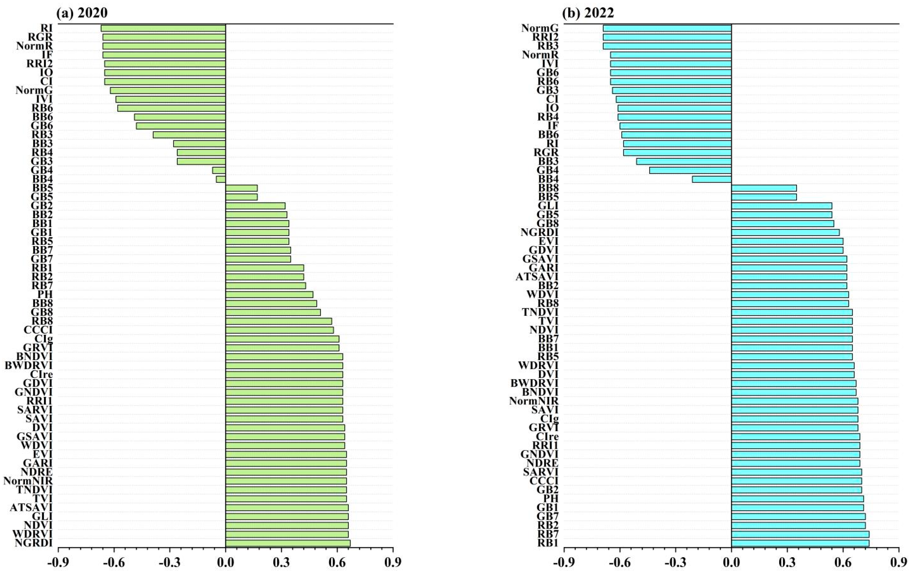
In this study, a total of 25 RGB features and 34 MS features were acquired from the relevant data sources. We conducted a Pearson correlation analysis on the 59 spectral features obtained for the years 2020 and 2022 to assess their relationships with yield.
As shown in Figure 4a, it is evident that the majority of spectral features exhibit robust and statistically significant correlations with yield for the year 2020. MS features exhibit a stronger correlation with yield than the RGB features. NGRDI and RI show the highest correlation, with an absolute value reaching 0.67. Figure 4b illustrates that all the spectral features exhibited pronounced and statistically significant correlations with yield in 2022. Interestingly, in that year, the correlation between the RGB features and yield was stronger than that of MS features. The correlation reached an absolute value of 0.74. When comparing the data from the two years in relation to yield, the spectral features showed a more robust correlation in 2022.
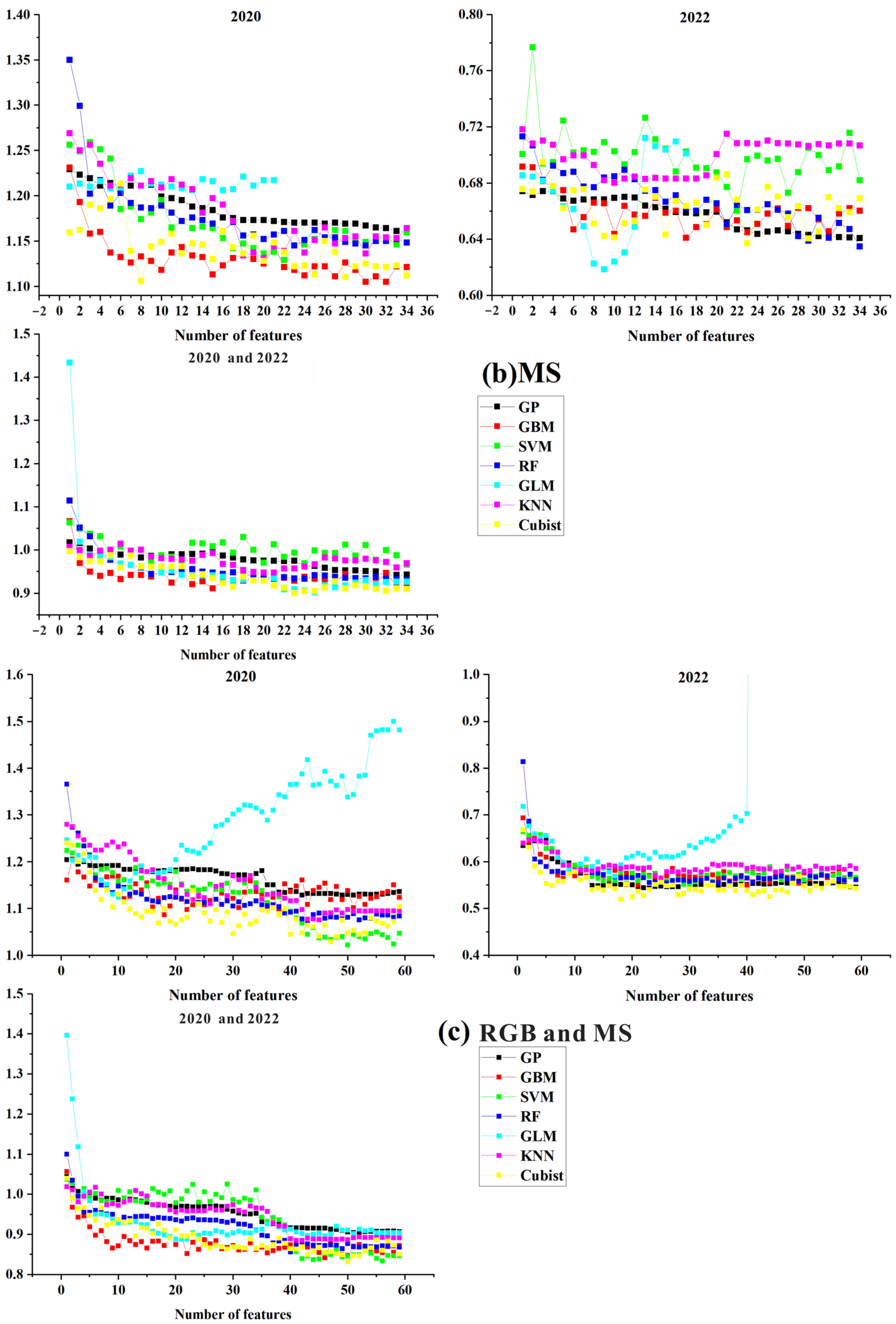
Although many spectral features showed significant and strong correlations with yield, the large number of features created in this study required a feature selection process. To streamline these for model building, we employed the RFE method. Therefore, we applied the RFE method to filter the RGB and MS features, MS features, and RGB features in the 2020, 2022, and 2020 and 2022 datasets using the seven machine learning algorithms. The RMSE regression loss of each algorithm was calculated. Figure 5 illustrates the relationship between the number of input features (on the x-axis) and the RMSE regression loss (on the y-axis). Different lines represent the variation across the folds. A lower RMSE indicates a higher prediction accuracy for the model. The optimal number of input features for each of the seven machine learning algorithms is detailed in Table 2.
The range of RMSE with increasing number of input features is narrow for all models except for the GLM model. In summary, the year 2022 had the lowest RMSE regression loss, ranging from 0.52 to 0.83 t·ha−1, indicating the best model fit. The dataset for 2020 and 2022 followed, with RMSE ranging from 0.8 to 1.5 t·ha−1. When RGB features were used as inputs, the Cubist model achieved the lowest RMSE of 0.52 t·ha−1 in 2022 with 18 features. Additionally, the Cubist model exhibited the minimum RMSE value in 2020 and 2022. For MS features, the RMSE in 2022 varied from 0.65 to 0.78 t·ha−1. The GLM model achieved the lowest RMSE of 0.619 t·ha−1 with nine features. When RGB and MS features were evaluated, the Cubist model again excelled, with an RMSE of 0.520 t·ha−1 with 18 features. Both the SVM and Cubist models exhibited their lowest RMSE values when 50 features were used as input for the 2020 and, 2020 and 2022 datasets.

3.3. Analysis of the Model Accuracy

The machine learning models underwent feature filtering using seven RFE methods for each of the nine datasets. BMA was employed to ensemble the seven machine learning models. The accuracy achieved by each model is shown in Table 3. Evaluating the accuracy of the eight models under nine input combinations, some conclusions can be drawn.
Among the seven individual machine learning models, the 2020 SVM model performed best, reaching an R2 of 0.597 with RGB and MS as input features. Notably, the 2022 and, 2020 and 2022 models, both employing the Cubist algorithm, excelled with significant R2 of 0.703 and 0.715, respectively, when utilizing RGB and MS features. This underscores the superior performance of the Cubist model for winter wheat yield analysis. Models with diverse input features achieved the highest R2. The R2 values for the 2020 model ranged from 0.445 to 0.597, while those for the 2022 model varied from 0.495 to 0.703. Additionally, the R2 for the 2020 and 2022 model consistently exceeded 0.6 in most cases, underscoring its robust performance across various scenarios. Importantly, the ensemble model’s accuracy consistently surpassed that of the individual 2020 and 2022 models.
The BMA prediction model was created by combining predictions from seven separate machine learning models, each developed independently. The model’s results, including R2 values, are presented in Table 3. Our analysis revealed that BMA models developed with varying input features consistently exhibited superior accuracy when compared to the individual machine learning models. Notably, the highest accuracy was achieved in the 2020 and 2022 model, boasting an impressive R2 of 0.725, with RMSE and MSE values of 0.815 t·ha−1 and 0.663 t·ha−1, respectively. Compared to the top-performing individual machine learning models with diverse input features, the BMA model showed a significant R2 improvement, ranging from 0.002 to 0.045. This robustly underscores the practical significance and superiority of the BMA model.

3.4. Model Generalizability Validation Analysis

To further validate the model’s performance, this study employed two distinct validation approaches, labeled A and B. Because the training and validation sets were already established, we could not use the RFE method to find the best input combination for the prediction model. Instead, the optimal input feature combination of each individual model was determined through the RFE method. Consequently, the prediction results obtained from the 2020 and 2022 dataset served as the input features for constructing the yield prediction model.
The accuracy of the seven individual machine learning models is presented in Table 4. SVM, RF, and KNN did not perform well in terms of accuracy. Their R2 values were below 0.48, and the RMSE exceeded 0.7 t·ha−1, with a maximum RMSE of 1.939 t·ha−1. The GBM model displayed some predictive capability when constructing the yield prediction model based on RGB features in validation approach A (R2 = 0.497, RMSE = 1.013 t·ha−1, MSE = 1.026 t·ha−1). In contrast, all Cubist and GLM models demonstrated reliable predictive performance, with R2 values exceeding 0.48. Among them, the Cubist model exhibited the best predictive performance (R2 = 0.634, RMSE = 0.593 t·ha−1, MSE = 0.352 t·ha−1). Overall, the models constructed using validation approach A generally exhibited higher accuracy than those using validation approach B. It was deduced that an R2 value below 0.48 may not provide reliable predictive performance. Only individual machine learning models with an R2 greater than 0.48 were used to build the BMA predictive models. Their accuracies are summarized in Table 4. Notably, the BMA models consistently outperformed any individual machine learning model. The highest prediction accuracy was achieved using validation approach A (R2 = 0.673, RMSE = 0.560 t·ha−1, MSE = 0.313 t·ha−1). Furthermore, the R2 values of the BMA models fell within the range of 0.51–0.673, while the RMSE values ranged from 0.313 to 1.170 t·ha−1, confirming the reliability of their predictive performance.

4. Discussion

4.1. Multi-Sensor Features

The selection and fusion of features from MS and RGB sensors offer significant advantages in scientific research. MS sensors capture data from various spectral bands, providing rich spectral features [62]. Conversely, RGB sensors offer high-resolution image information [63]. Combining features extracted from these two sensor types, we leverage their strengths to create a more accurate representation. Feature fusion amalgamates the advantages of MS and RGB sensors, enhancing prediction accuracy and stability in regression models. Most models in this study showed improved accuracy when RGB and MS features were fused, aligning with previous findings [38]. Feature fusion also addresses limitations of individual sensors [64]. These limitations include insensitivity to specific spectral bands in MS sensors and susceptibility to lighting conditions and color distortion in RGB sensors [65]. Combining features, we compensate for these shortcomings. This approach improves adaptability to different scenarios and data variations. Using fused multi-sensor features from 2020 and 2022, each model demonstrated better adaptability compared to single-sensor features, with slightly higher R2 values. Additionally, feature fusion expanded the dataset, increasing the number of input features and training samples, which improved generalization ability and stability. It is important to note that this study exclusively utilized features from two sensors. Future research can explore incorporating thermal infrared, hyperspectral, and other sensor features. This exploration aims to further enhance predictive capabilities and conduct more comprehensive investigations.

4.2. Advantages of the RFE Approach Based on Multiple Individual Models

Multi-model RFE is a valuable strategy for achieving more accurate and robust results in model building and prediction. In this approach, the evaluation of feature importance using multiple base models plays a crucial role [66]. The base models chosen in this study encompass linear models, tree models, and support vector machines. Each of these models provides distinct indicators of feature importance. Through the utilization of multiple base models, we obtain a comprehensive and diverse evaluation of feature importance. Different individual models possess the capability to capture various types of feature relationships and non-linear associations. This diversity leads to a more accurate ranking of feature importance. In this study, the amalgamation of feature importance from multiple base models helps mitigate biases or errors that may arise from a single model. This approach ultimately enhances the stability and reliability of feature selection. This is in alignment with previous findings [67]. Throughout the process of RFE, we iteratively remove features contributing less to the model’s prediction. This gradual reduction of the feature space allows us to obtain a more concise feature combination. This aids in the reduction of feature dimensionality, minimizes model complexity, and improves model interpretability [68]. The iterative selection of the best feature combination offers flexibility in the number of features included. This flexibility is observed in the feature selection methods based on different base models (Table 2). This approach significantly enhances the model’s generalization ability and prediction accuracy. Furthermore, the implementation of RFE methods based on multiple base models diminishes the risk of overfitting [69]. The gradual elimination of unimportant features substantially decreases the model’s sensitivity to noise and redundant features. This process results in improved model robustness and stability.

4.3. Advantages of Individual Machine Learning Models

The utilization of seven different machine learning algorithms enables a comprehensive approach to data modeling and analysis. Each algorithm operates uniquely, capturing diverse data patterns and associations [70]. For example, tree-based algorithms excel at handling non-linear relationships [71,72], while support vector machines are effective at managing high-dimensional data [71,73]. Combining these algorithms, we can thoroughly explore the dataset’s features and patterns, enhancing the flexibility and adaptability of the prediction models. Moreover, employing multiple machine learning algorithms helps mitigate the limitations and biases associated with relying on a single algorithm. It is observed that no single model consistently outperforms others when constructed under varying conditions and using different data characteristics. This highlights that each machine learning algorithm operates under its own set of assumptions and limitations [74]. Using multiple algorithms enables the construction of models across diverse conditions, facilitating model comparison and selection. Assessing how different algorithms perform on the same dataset helps identify their strengths, weaknesses, and suitability for yield prediction. This aids in choosing the most effective algorithm or a combination of algorithms. In this study, the Cubist model demonstrated promising predictive performance across different scenarios, achieving a maximum R2 of 0.715. Additionally, the utilization of multiple machine learning algorithms enables the exploration of the importance and influence of feature factors. The assessment of feature importance may vary among algorithms. Comparing the feature selection outcomes of multiple algorithms, we gain insights into the extent to which different features contribute to yield prediction. This optimization of feature selection and model interpretation capabilities enhances our understanding of the significance of various features in the context of yield prediction [75].

4.4. Advantages of the BMA Model

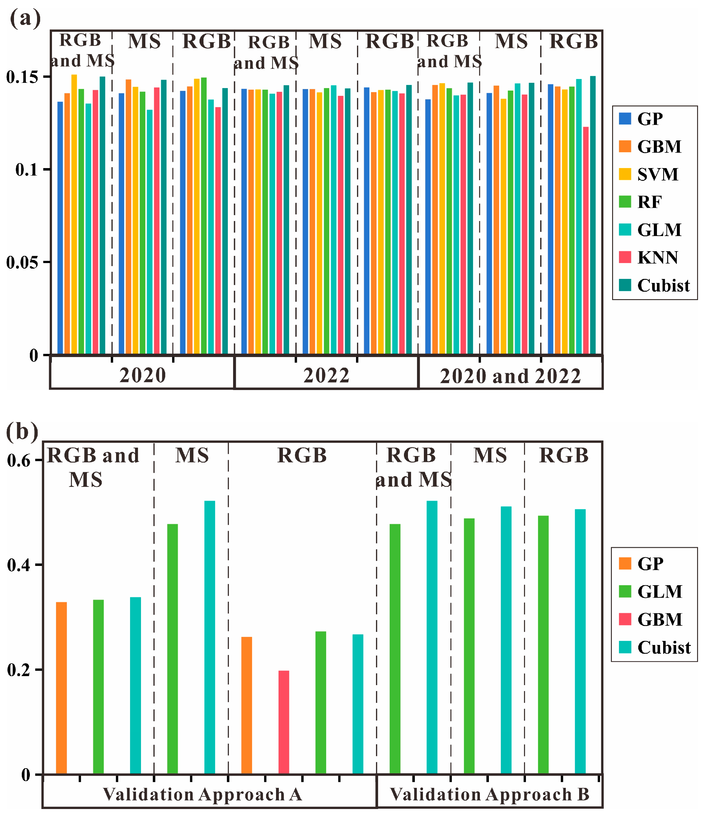
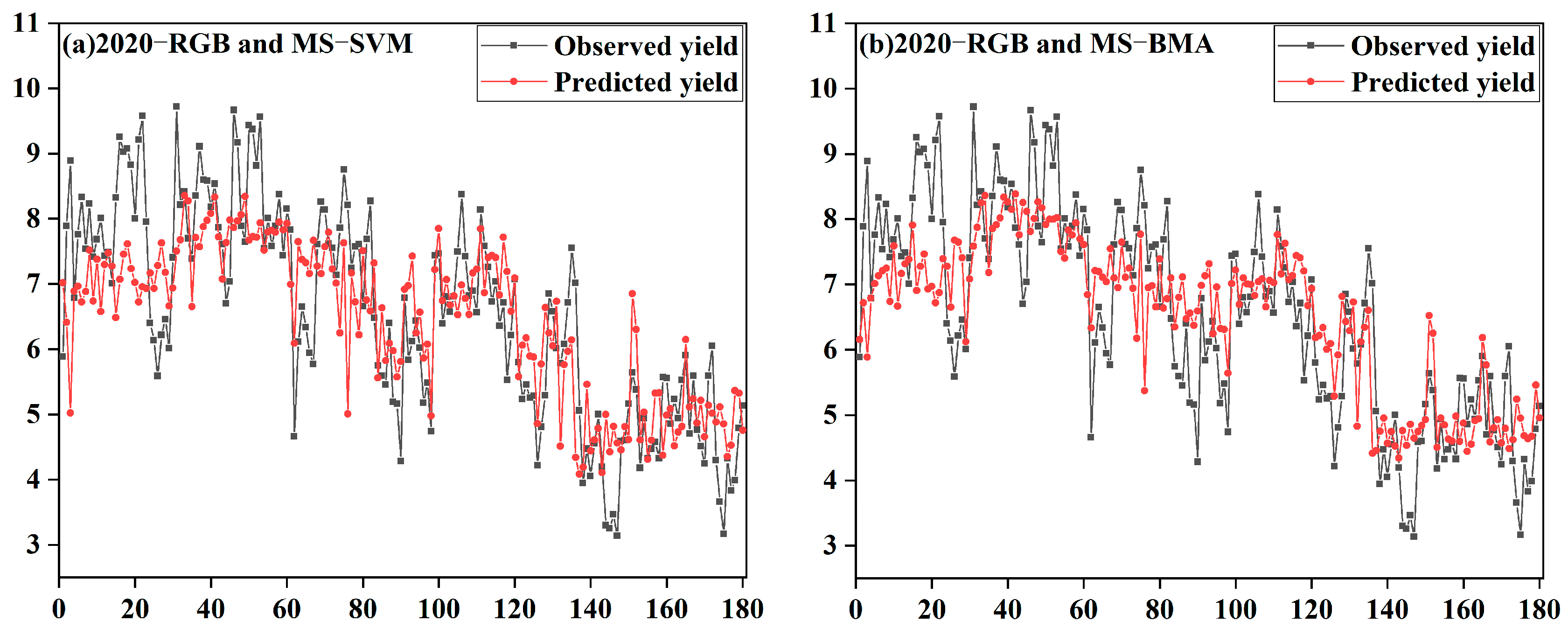
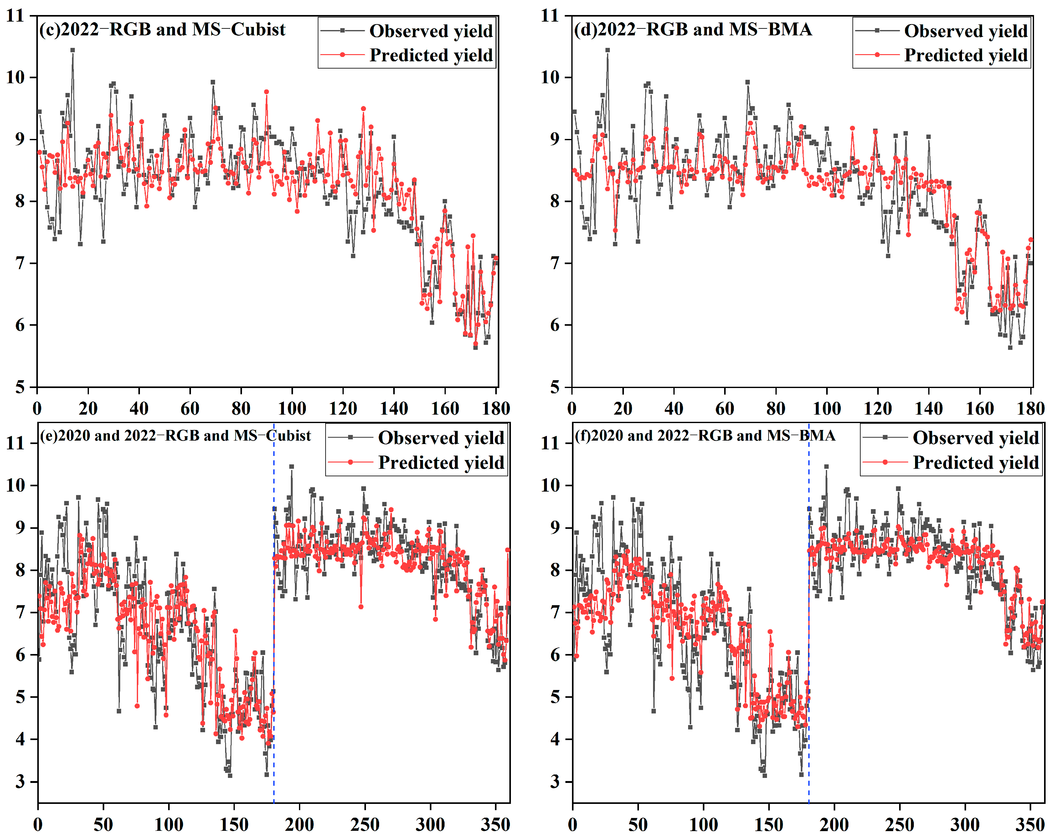
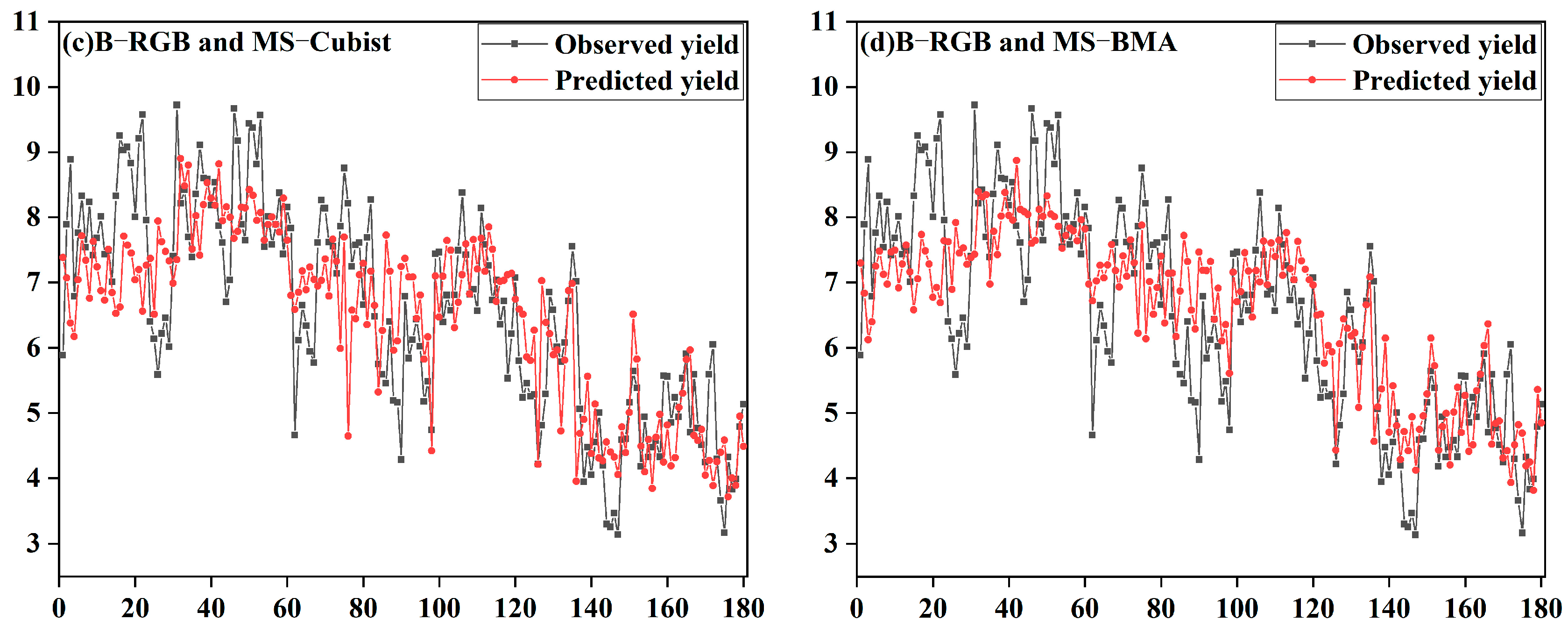
The BMA model utilized in this study achieved reliable yield predictions with improved accuracy compared to the seven independent machine learning models. The highest R2 increased to 0.725, and the lowest RMSE decreased to 0.258. The BMA model’s success can be attributed to two main factors. Firstly, it efficiently extracted information from seven existing machine learning models, avoiding uncertainties associated with individual model parameters and structures [33]. Secondly, the BMA model derives prior probabilities based on the performance of each individual model, enhancing prediction accuracy by aggregating models with strong performance [76]. Figure 6 illustrates the normalized weights of each individual machine learning model in constructing the BMA model. The SVM model holds the highest weight in the 2020 dataset, while the Cubist model carries the greatest weight in both the 2022 and, 2020 and 2022 datasets. Notably, these individual machine learning models are the top performers, as confirmed in validation approaches A and B. This demonstrates that the BMA model leverages the best-performing models to enhance accuracy and reliability, consistent with the findings in a previous study [36]. Figure 7 displays the observed and predicted values of the best individual machine learning models and BMA models constructed using data from different years. Examining the optimal separate prediction models for the three datasets reveals that the difference between the predicted and observed values fluctuates within a specific range. The smallest fluctuation range is observed in the 2022 dataset, ranging from −1.99 to 2.20 t·ha−1. For the BMA model, the fluctuation range of the difference between predicted and observed values is even smaller, fluctuating between −1.54 and 2.24 t·ha−1. Figure 8 presents the observed and predicted values of the yield prediction models, based on validation methods A and B. Both the optimal individual machine learning model and the BMA model are included for comparison. It is evident that the fluctuation range of the difference between the predicted and observed values is smaller for the BMA model compared to the individual machine learning model. Furthermore, the fluctuation range for validation approach A is significantly reduced compared to validation approach B. This demonstrates that the BMA model effectively reduces model uncertainties, enhancing its overall reliability. Additionally, the results obtained from validation methods A and B indicate that the BMA model consistently outperforms the standalone machine learning model on unseen datasets. This highlights the superior generalization ability of the BMA model. Furthermore, the novel approaches used in this study show promise, the data collected from only one sampling time (grain filling stage) may not be sufficient to provide highly accurate yield predictions. Therefore, the sampling times selected for this study were 6 May 2020 and 10 May 2022, both at similar nodes during the grain filling period of winter wheat. This enabled us to explore the performance of yield prediction models at the same fertility nodes in different environments. In the future, studies could consider multiple sampling sessions throughout the growing season to enhance the robustness of the data and improve prediction accuracy. We observed significant variation and dispersion between the observed and predicted yields. The observed discrepancies may be attributed to the inherent variability in plant growth conditions.

4.5. Analysis of Model Generalization Capabilities

Utilizing a one-year training set and a one-year validation set represents a common approach for evaluating the generalizability and generalization capacity of machine learning models. This method effectively assesses model performance on unseen data, ensuring the model’s reliability for real-world applications. Initially, constructing the model using two years of data allows for the incorporation of historical insights and trends, leading to enhanced accuracy and stability [77]. Training the model on a two-year dataset allows it to consider factors like seasonality and environmental conditions. This approach results in a more comprehensive and representative model [31]. Additionally, employing one year’s data as the training set in this study enables the model to learn historical patterns and correlation patterns, ensuring a proper fit to the data. Using another year’s data as the validation set tests the model’s performance on new data, assessing its ability to generalize and remain stable. Among the models created using validation methods A and B, the Cubist and GLM models show the best predictive abilities. In contrast, the RF model, despite having the highest accuracy, exhibits poor predictive performance and struggles to provide reliable predictions. This outcome may be attributed to the model’s one-year training data not aligning well with the unseen data or a lack of features. Subsequent studies will consider incorporating more than three years of data for in-depth exploration.

5. Conclusions

In this study, we developed yield prediction models using RFE methods, seven individual machine learning algorithms, and the BMA ensemble learning algorithm. The models, developed from UAV-collected RGB and MS features in 2020 and 2022, consistently demonstrated high accuracy. Whether using RGB features, MS features, or RGB + MS features, all seven models showed reliable performance. Among the models constructed with recursive feature selection, the Cubist model demonstrated the best performance (R2 = 0.715, RMSE = 0.831 t·ha−1, MSE = 0.691 t·ha−1). Furthermore, the BMA model consistently outperformed the individual machine learning models in all cases, achieving a maximum R2 of 0.725. Training our yield prediction models with data from one year and validating them with data from another year proved effective. Notably, the Cubist and GLM models displayed robust predictive performance. The BMA model continued to surpass the performance of the individual machine learning models, achieving the highest accuracy in validation approach A (R2 = 0.673, RMSE = 0.560 t·ha−1, MSE = 0.313 t·ha−1). This demonstrates the superior generalization ability of the BMA model, making it a promising choice for future research involving multi-year data prediction.

Author Contributions

Conceptualization: Z.C., X.Z. and Z.L.; trial management and data collection and analysis: Z.L., Q.C., Z.C. and L.C.; writing under supervision of Z.C. and X.Z.; editing: Z.L., Z.C., X.Z. and Q.C; formal analysis: B.Z. and S.G. All authors have read and agreed to the published version of the manuscript.

Funding

This research was funded by the Key Grant Technology Project of Henan (221100110700), National Key R&D Program of China (2023YFD1900705), the Central Public-interest Scientific Institution Basal Research Fund (No. IFI2024-01), and the Agricultural Science and Technology Innovation Program (ASTIP No. CAAS-ZDRW202201).

Data Availability Statement

The raw data supporting the conclusions of this article will be made available by the authors on request.

Conflicts of Interest

The authors assert that they have no conflicts of interest regarding this study.

References

  1. Fu, Z.; Jiang, J.; Gao, Y.; Krienke, B.; Wang, M.; Zhong, K.; Cao, Q.; Tian, Y.; Zhu, Y.; Cao, W.; et al. Wheat Growth Monitoring and Yield Estimation based on Multi-Rotor Unmanned Aerial Vehicle. Remote Sens. 2020, 12, 508. [Google Scholar] [CrossRef]
  2. Maes, W.H.; Steppe, K. Perspectives for Remote Sensing with Unmanned Aerial Vehicles in Precision Agriculture. Trends Plant Sci. 2019, 24, 152–164. [Google Scholar] [CrossRef] [PubMed]
  3. Diaz-Gonzalez, F.A.; Vuelvas, J.; Correa, C.A.; Vallejo, V.E.; Patino, D. Machine learning and remote sensing techniques applied to estimate soil indicators—Review. Ecol. Indic. 2022, 135, 108517. [Google Scholar] [CrossRef]
  4. Katsigiannis, P.; Galanis, G.; Dimitrakos, A.; Tsakiridis, N.; Kalopesas, C.; Alexandridis, T.; Chouzouri, A.; Patakas, A.; Zalidi, G. Fusion of Spatio-Temporal UAV and Proximal Sensing Data for an Agricultural Decision Support System. In Proceedings of the Fourth International Conference on Remote Sensing and Geoinformation of the Environment (RSCY2016), Paphos, Cyprus, 4–8 April 2016; Volume 1, p. 9688. [Google Scholar]
  5. Loots, M.; Grobbelaar, S.; van der Lingen, E. A review of remote-sensing unmanned aerial vehicles in the mining industry. J. S. Afr. Inst. Min. Metall. 2022, 122, 387–396. [Google Scholar] [CrossRef]
  6. Huang, W.; Lu, J.; Ye, H.; Kong, W.; Mortimer, A.H.; Shi, Y. Quantitative identification of crop disease and nitrogen-water stress in winter wheat using continuous wavelet analysis. Int. J. Agric. Biol. Eng. 2018, 11, 145–152. [Google Scholar] [CrossRef]
  7. Primicerio, J.; Di Gennaro, S.F.; Fiorillo, E.; Genesio, L.; Lugato, E.; Matese, A.; Vaccari, F.P. A flexible unmanned aerial vehicle for precision agriculture. Precis. Agric. 2012, 13, 517–523. [Google Scholar] [CrossRef]
  8. Nijland, W.; de Jong, R.; de Jong, S.M.; Wulder, M.A.; Bater, C.W.; Coops, N.C. Monitoring plant condition and phenology using infrared sensitive consumer grade digital cameras. Agric. For. Meteorol. 2014, 184, 98–106. [Google Scholar] [CrossRef]
  9. Zheng, H.; Cheng, T.; Li, D.; Zhou, X.; Yao, X.; Tian, Y.; Cao, W.; Zhu, Y. Evaluation of RGB, Color-Infrared and Multispectral Images Acquired from Unmanned Aerial Systems for the Estimation of Nitrogen Accumulation in Rice. Remote Sens. 2018, 10, 824. [Google Scholar] [CrossRef]
  10. Mahlein, A. Plant Disease Detection by Imaging Sensors—Parallels and Specific Demands for Precision Agriculture and Plant Phenotyping. Plant Dis. 2016, 100, 241–251. [Google Scholar] [CrossRef]
  11. Prashar, A.; Jones, H.G. Assessing Drought Responses Using Thermal Infrared Imaging. In Methods in Molecular Biology; Duque, P., Ed.; Springer Nature: Shanghai, China, 2016; Volume 1398, pp. 209–219. [Google Scholar]
  12. Prey, L.; Hanemann, A.; Ramgraber, L.; Seidl-Schulz, J.; Noack, P.O. UAV-Based Estimation of Grain Yield for Plant Breeding: Applied Strategies for Optimizing the Use of Sensors, Vegetation Indices, Growth Stages, and Machine Learning Algorithms. Remote Sens. 2022, 14, 6345. [Google Scholar] [CrossRef]
  13. Geipel, J.; Link, J.; Wirwahn, J.A.; Claupein, W. A Programmable Aerial Multispectral Camera System for In-Season Crop Biomass and Nitrogen Content Estimation. Agriculture 2016, 6, 4. [Google Scholar] [CrossRef]
  14. Honkavaara, E.; Saari, H.; Kaivosoja, J.; Polonen, I.; Hakala, T.; Litkey, P.; Makynen, J.; Pesonen, L. Processing and Assessment of Spectrometric, Stereoscopic Imagery Collected Using a Lightweight UAV Spectral Camera for Precision Agriculture. Remote Sens. 2013, 5, 5006–5039. [Google Scholar] [CrossRef]
  15. Lohmann, G. Analysis and synthesis of textures—A co-occurrence-based approach. Comput. Graph. 1995, 19, 29–36. [Google Scholar] [CrossRef]
  16. Yue, J.; Yang, G.; Tian, Q.; Feng, H.; Xu, K.; Zhou, C. Estimate of winter-wheat above-ground biomass based on UAV ultrahigh-ground-resolution image textures and vegetation indices. ISPRS J. Photogramm. Remote Sens. 2019, 150, 226–244. [Google Scholar] [CrossRef]
  17. Zheng, H.; Cheng, T.; Zhou, M.; Li, D.; Yao, X.; Tian, Y.; Cao, W.; Zhu, Y. Improved estimation of rice aboveground biomass combining textural and spectral analysis of UAV imagery. Precis. Agric. 2019, 20, 611–629. [Google Scholar] [CrossRef]
  18. Poley, L.G.; McDermid, G.J. A Systematic Review of the Factors Influencing the Estimation of Vegetation Aboveground Biomass Using Unmanned Aerial Systems. Remote Sens. 2020, 12, 1052. [Google Scholar] [CrossRef]
  19. Cao, J.; Leng, W.; Liu, K.; Liu, L.; He, Z.; Zhu, Y. Object-Based Mangrove Species Classification Using Unmanned Aerial Vehicle Hyperspectral Images and Digital Surface Models. Remote Sens. 2018, 10, 89. [Google Scholar] [CrossRef]
  20. Kotoku, J. An Introduction to Machine Learning. Igaku Butsuri Nihon Igaku Butsuri Gakkai Kikanshi Jpn. J. Med. Phys. 2016, 36, 18–22. [Google Scholar]
  21. Revill, A.; Florence, A.; MacArthur, A.; Hoad, S.; Rees, R.; Williams, M. Quantifying Uncertainty and Bridging the Scaling Gap in the Retrieval of Leaf Area Index by Coupling Sentinel-2 and UAV Observations. Remote Sens. 2020, 12, 1843. [Google Scholar] [CrossRef]
  22. Barzin, R.; Kamangir, H.; Bora, G.C. Comparison of machine learning methods for leaf nitrogen estimation in corn using multispectral uav images. Trans. ASABE 2021, 64, 2089–2101. [Google Scholar] [CrossRef]
  23. Proietti, T.; Luati, A. Generalized linear cepstral models for the spectrum of a time series. Stat. Sin. 2019, 29, 1561–1583. [Google Scholar]
  24. Li, Y. SVM-based Weed Identification Using Field Imaging Spectral Data. Remote Sens. Inf. 2014, 29, 40–43,50. [Google Scholar]
  25. Silva, E.B.; Giasson, E.; Dotto, A.C.; Ten Caten, A.; Melo Dematte, J.A.; Bacic, I.L.Z.; Da Veiga, M. A Regional Legacy Soil Dataset for Prediction of Sand and Clay Content with Vis-Nir-Swir, in Southern Brazil. Rev. Bras. Cienc. Solo 2019, 43, e0180174. [Google Scholar] [CrossRef]
  26. Cao, Q.; Xu, D.; Ju, H. Biomass estimation of five kinds of mangrove community with the KNN method based on the spectral information and textural features of TM images. For. Res. 2011, 24, 144–150. [Google Scholar]
  27. Yang, H.; Hu, Y.; Zheng, Z.; Qiao, Y.; Zhang, K.; Guo, T.; Chen, J. Estimation of Potato Chlorophyll Content from UAV Multispectral Images with Stacking Ensemble Algorithm. Agronomy 2022, 12, 2318. [Google Scholar] [CrossRef]
  28. Li, Z.; Chen, Z.; Cheng, Q.; Duan, F.; Sui, R.; Huang, X.; Xu, H. UAV-Based Hyperspectral and Ensemble Machine Learning for Predicting Yield in Winter Wheat. Agronomy 2022, 12, 202. [Google Scholar] [CrossRef]
  29. Lin, X.; Chen, J.; Lou, P.; Yi, S.; Qin, Y.; You, H.; Han, X. Improving the estimation of alpine grassland fractional vegetation cover using optimized algorithms and multi-dimensional features. Plant Methods 2021, 17, 96. [Google Scholar] [CrossRef] [PubMed]
  30. Wang, F.; Yi, Q.; Xie, L.; Yao, X.; Zheng, J.; Xu, T.; Li, J.; Chen, S. Non-destructive monitoring of amylose content in rice by UAV-based hyperspectral images. Front. Plant Sci. 2022, 13, 1035379. [Google Scholar] [CrossRef] [PubMed]
  31. Zheng, H.; Cheng, T.; Li, D.; Yao, X.; Tian, Y.; Cao, W.; Zhu, Y. Combining Unmanned Aerial Vehicle (UAV)-Based Multispectral Imagery and Ground-Based Hyperspectral Data for Plant Nitrogen Concentration Estimation in Rice. Front. Plant Sci. 2018, 9, 936. [Google Scholar] [CrossRef]
  32. Qiao, L.; Zhao, R.; Tang, W.; An, L.; Sun, H.; Li, M.; Wang, N.; Liu, Y.; Liu, G. Estimating maize LAI by exploring deep features of vegetation index map from UAV multispectral images. Field Crops Res. 2022, 289, 108739. [Google Scholar] [CrossRef]
  33. Liu, Z.; Merwade, V. Separation and prioritization of uncertainty sources in a raster based flood inundation model using hierarchical Bayesian model averaging. J. Hydrol. 2019, 578, 124100. [Google Scholar] [CrossRef]
  34. Ossandon, A.; Rajagopalan, B.; Lall, U.; Nanditha, J.S.; Mishra, V. A Bayesian Hierarchical Network Model for Daily Streamflow Ensemble Forecasting. Water Resour. Res. 2021, 57, e2021WR029920. [Google Scholar] [CrossRef]
  35. Mustafa, S.M.T.; Nossent, J.; Ghysels, G.; Huysmans, M. Estimation and Impact Assessment of Input and Parameter Uncertainty in Predicting Groundwater Flow with a Fully Distributed Model. Water Resour. Res. 2018, 54, 6585–6608. [Google Scholar] [CrossRef]
  36. Zhou, T.; Wen, X.; Feng, Q.; Yu, H.; Xi, H. Bayesian Model Averaging Ensemble Approach for Multi-Time-Ahead Groundwater Level Prediction Combining the GRACE, GLEAM, and GLDAS Data in Arid Areas. Remote Sens. 2023, 15, 188. [Google Scholar] [CrossRef]
  37. Huang, H.; Liang, Z.; Li, B.; Wang, D.; Hu, Y.; Li, Y. Combination of Multiple Data-Driven Models for Long-Term Monthly Runoff Predictions Based on Bayesian Model Averaging. Water Resour. Manag. 2019, 33, 3321–3338. [Google Scholar] [CrossRef]
  38. Li, Z.; Zhou, X.; Cheng, Q.; Fei, S.; Chen, Z. A Machine-Learning Model Based on the Fusion of Spectral and Textural Features from UAV Multi-Sensors to Analyse the Total Nitrogen Content in Winter Wheat. Remote Sens. 2023, 15, 2152. [Google Scholar] [CrossRef]
  39. Hancock, D.W.; Dougherty, C.T. Relationships between blue- and red-based vegetation indices and leaf area and yield of alfalfa. Crop Sci. 2007, 47, 2547–2556. [Google Scholar] [CrossRef]
  40. Gitelson, A.A.; Kaufman, Y.J.; Stark, R.; Rundquist, D. Novel algorithms for remote estimation of vegetation fraction. Remote Sens. Environ. 2002, 80, 76–87. [Google Scholar] [CrossRef]
  41. Gamon, J.A.; Surfus, J.S. Assessing leaf pigment content and activity with a reflectometer. New Phytol. 1999, 143, 105–117. [Google Scholar] [CrossRef]
  42. Ehammer, A.; Fritsch, S.; Conrad, C.; Lamers, J.; Dech, S. Statistical derivation of fPAR and LAI for irrigated cotton and rice in arid Uzbekistan by combining multi-temporal RapidEye data and ground measurements. In Proceedings of the Remote Sensing for Agriculture, Ecosystems, and Hydrology XII, Toulouse, France, 20–22 September 2010; Volume 7824. [Google Scholar]
  43. Bastiaanssen, W.; Molden, D.J.; Makin, I.W. Remote sensing for irrigated agriculture: Examples from research and possible applications. Agric. Water Manag. 2000, 46, 137–155. [Google Scholar] [CrossRef]
  44. Broge, N.H.; Leblanc, E. Comparing prediction power and stability of broadband and hyperspectral vegetation indices for estimation of green leaf area index and canopy chlorophyll density. Remote Sens. Environ. 2001, 76, 156–172. [Google Scholar] [CrossRef]
  45. Hunt, E.R., Jr.; Daughtry, C.S.T.; Eitel, J.U.H.; Long, D.S. Remote Sensing Leaf Chlorophyll Content Using a Visible Band Index. Agron. J. 2011, 103, 1090–1099. [Google Scholar] [CrossRef]
  46. Wu, C.; Niu, Z.; Tang, Q.; Huang, W.; Rivard, B.; Feng, J. Remote estimation of gross primary production in wheat using chlorophyll-related vegetation indices. Agric. For. Meteorol. 2009, 149, 1015–1021. [Google Scholar] [CrossRef]
  47. Hewson, R.D.; Cudahy, T.J.; Huntington, J.F. Geologic and alteration mapping at Mt Fitton, South Australia, using ASTER satellite-borne data. In Proceedings of the IGARSS 2001: Scanning the Present and Resolving the Future, Proceedings, Sydney, NSW, Australia, 9–13 July 2001; Volumes 1–7, pp. 724–726. [Google Scholar]
  48. Tran, T.V.; Reef, R.; Zhu, X. A Review of Spectral Indices for Mangrove Remote Sensing. Remote Sens. 2022, 14, 4868. [Google Scholar] [CrossRef]
  49. Ahamed, T.; Tian, L.; Zhang, Y.; Ting, K.C. A review of remote sensing methods for biomass feedstock production. Biomass Bioenergy 2011, 35, 2455–2469. [Google Scholar] [CrossRef]
  50. LUO, Y.; XU, J.; YUE, W.; CHEN, W. A Comparative Study of Extracting Urban Vegetation Information by Vegetation Indices from Thematic Mapper Images. Remote Sens. Technol. Appl. 2006, 21, 212–219. [Google Scholar]
  51. Tucker, C.J.; Elgin, J.H., Jr.; McMurtrey, J.E.I.; Fan, C.J. Monitoring corn and soybean crop development with hand-held radiometer spectral data. Remote Sens. Environ. 1979, 8, 237–248. [Google Scholar] [CrossRef]
  52. Da Luz, A.G.; Bleninger, T.B.; Polli, B.A.; Lipski, B. Spatio-temporal variation of aquatic macrophyte cover in a reservoir using Landsat images and Google Earth Engine. RBRH-Revista Brasileira De Recursos Hidricos 2022, 27, e37. [Google Scholar] [CrossRef]
  53. Abdollahi, A.; Zakeri, N. Cospectrality of multipartite graphs. Ars Math. Contemp. 2022, 22, 1. [Google Scholar] [CrossRef]
  54. Del Portal, F.R.; Salazar, J.M. Shape index in metric spaces. Fundam. Math. 2003, 176, 47–62. [Google Scholar] [CrossRef]
  55. Rajapakse, J.C.; Duan, K.B.; Yeo, W.K. Proteomic cancer classification with mass spectrometry data. Am. J. Pharmacogenom. 2005, 5, 281–292. [Google Scholar] [CrossRef] [PubMed]
  56. Ding, J.; Shi, J.; Wu, F. SVM-RFE based feature selection for tandem mass spectrum quality assessment. Int. J. Data Min. Bioinform. 2011, 5, 73–88. [Google Scholar] [CrossRef] [PubMed]
  57. Rehman, T.U.; Mahmud, M.S.; Chang, Y.K.; Jin, J.; Shin, J. Current and future applications of statistical machine learning algorithms for agricultural machine vision systems. Comput. Electron. Agric. 2019, 156, 585–605. [Google Scholar] [CrossRef]
  58. Payne, R.W. Developments from analysis of variance through to generalized linear models and beyond. Ann. Appl. Biol. 2014, 164, 11–17. [Google Scholar] [CrossRef]
  59. Fernandez-Delgado, M.; Sirsat, M.S.; Cernadas, E.; Alawadi, S.; Barro, S.; Febrero-Bande, M. An extensive experimental survey of regression methods. Neural Netw. 2019, 111, 11–34. [Google Scholar] [CrossRef] [PubMed]
  60. Zhou, Y.; Wu, Z.; Xu, H.; Wang, H. Prediction and early warning method of inundation process at waterlogging points based on Bayesian model average and data-driven. J. Hydrol.-Reg. Stud. 2022, 44, 101248. [Google Scholar] [CrossRef]
  61. Garner, G.G.; Thompson, A.M. Ensemble statistical post-processing of the National Air Quality Forecast Capability: Enhancing ozone forecasts in Baltimore, Maryland. Atmos. Environ. 2013, 81, 517–522. [Google Scholar] [CrossRef]
  62. Vivone, G. Multispectral and hyperspectral image fusion in remote sensing: A survey. Inf. Fusion 2023, 89, 405–417. [Google Scholar] [CrossRef]
  63. Kim, J.; Chung, Y. A short review of RGB sensor applications for accessible high-throughput phenotyping. J. Crop Sci. Biotechnol. 2021, 24, 495–499. [Google Scholar] [CrossRef]
  64. Zhang, J. Multi-Source Remote Sensing Data Fusion: Status And Trends. Int. J. Image Data Fusion 2010, 1, 5–24. [Google Scholar] [CrossRef]
  65. Wu, D.; Li, R.; Zhang, F.; Liu, J. A review on drone-based harmful algae blooms monitoring. Environ. Monit. Assess. 2019, 191, 2114. [Google Scholar] [CrossRef] [PubMed]
  66. Yin, Y.; Jang-Jaccard, J.; Xu, W.; Singh, A.; Zhu, J.; Sabrina, F.; Kwak, J. IGRF-RFE: A hybrid feature selection method for MLP-based network intrusion detection on UNSW-NB15 dataset. J. Big Data 2023, 10, 15. [Google Scholar] [CrossRef]
  67. Zhou, R.; Yang, C.; Li, E.; Cai, X.; Yang, J.; Xia, Y. Object-Based Wetland Vegetation Classification Using Multi-Feature Selection of Unoccupied Aerial Vehicle RGB Imagery. Remote Sens. 2021, 13, 4910. [Google Scholar] [CrossRef]
  68. Jeon, H.; Oh, S. Hybrid-Recursive Feature Elimination for Efficient Feature Selection. Appl. Sci. 2020, 10, 3211. [Google Scholar] [CrossRef]
  69. Chen, X.; Jeong, J.C. Enhanced recursive feature elimination. In Proceedings of the ICMLA 2007: Sixth International Conference on Machine Learning and Applications, Proceedings, Cincinnati, OH, USA, 13–15 December 2007; pp. 429–435. [Google Scholar]
  70. Bastanlar, Y.; Ozuysal, M. Introduction to Machine Learning. In Methods in Molecular Biology; Yousef, M., Allmer, J., Eds.; Springer Nature: Shanghai, China, 2014; Volume 1107, pp. 105–128. [Google Scholar]
  71. Maimaitijiang, M.; Sagan, V.; Sidike, P.; Daloye, A.M.; Erkbol, H.; Fritschi, F.B. Crop Monitoring Using Satellite/UAV Data Fusion and Machine Learning. Remote Sens. 2020, 12, 1357. [Google Scholar] [CrossRef]
  72. Prodhan, F.A.; Zhang, J.; Hasan, S.S.; Sharma, T.P.P.; Mohana, H.P. A review of machine learning methods for drought hazard monitoring and forecasting: Current research trends, challenges, and future research directions. Environ. Model. Softw. 2022, 149, 105327. [Google Scholar] [CrossRef]
  73. Ishida, T.; Kurihara, J.; Angelico Viray, F.; Baes Namuco, S.; Paringit, E.C.; Jane Perez, G.; Takahashi, Y.; Joseph Marciano, J., Jr. A novel approach for vegetation classification using UAV-based hyperspectral imaging. Comput. Electron. Agric. 2018, 144, 80–85. [Google Scholar] [CrossRef]
  74. Qun’Ou, J.; Lidan, X.; Siyang, S.; Meilin, W.; Huijie, X. Retrieval Model For Total Nitrogen Concentration Based On Uav Hyper Spectral Remote Sensing Data And Machine Learning Algorithms—A Case Study In The Miyun Reservoir, China. Ecol. Indic. 2021, 124, 107356. [Google Scholar] [CrossRef]
  75. Guo, Q.; Zhang, J.; Guo, S.; Ye, Z.; Deng, H.; Hou, X.; Zhang, H. Urban Tree Classification Based on Object-Oriented Approach and Random Forest Algorithm Using Unmanned Aerial Vehicle (UAV) Multispectral Imagery. Remote Sens. 2022, 14, 3885. [Google Scholar] [CrossRef]
  76. Yin, J.; Medellin-Azuara, J.; Escriva-Bou, A.; Liu, Z. Bayesian machine learning ensemble approach to quantify model uncertainty in predicting groundwater storage change. Sci. Total Environ. 2021, 769, 144715. [Google Scholar] [CrossRef]
  77. Wang, F.; Yi, Q.; Hu, J.; Xie, L.; Yao, X.; Xu, T.; Zheng, J. Combining spectral and textural information in UAV hyperspectral images to estimate rice grain yield. Int. J. Appl. Earth Obs. Geoinf. 2021, 102, 102397. [Google Scholar] [CrossRef]
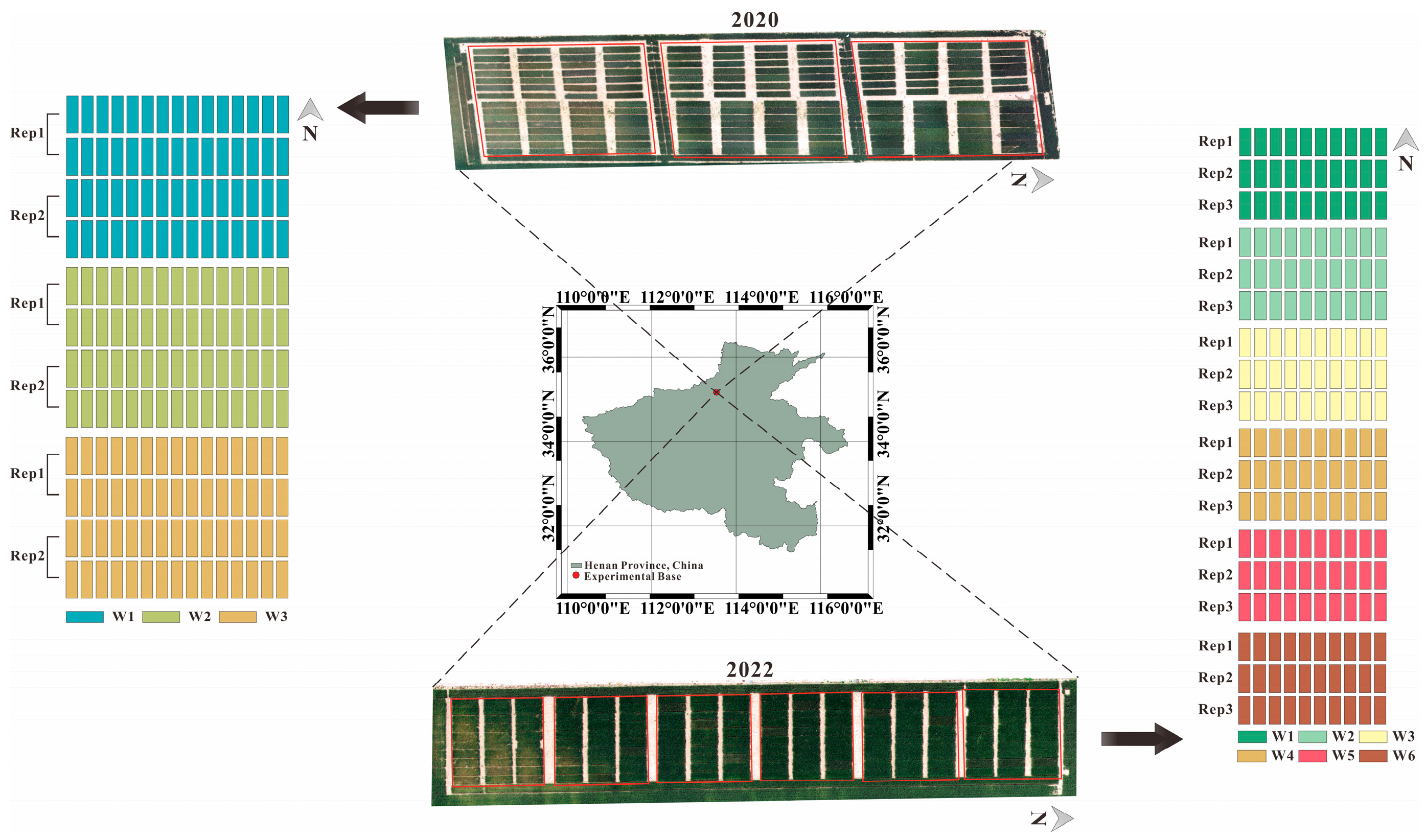
Figure 1. Test area and plots.
Remotesensing 16 02098 g001
Figure 2. Research framework and flow chart.
Remotesensing 16 02098 g002
Figure 3. Observed yield distribution in 2020 and 2022. (a) represents observed yield in 2020, (b) represents observed yield in 2022.
Remotesensing 16 02098 g003
Figure 4. Correlation of features and yield for 2020 and 2022. GB is green band texture; RB is red band texture and BB is blue band texture. Features are listed on the vertical axis, with positive correlations extending to the right and negative correlations to the left. Higher positive values suggest a stronger positive correlation with yield, while higher negative values indicate a stronger negative correlation.
Remotesensing 16 02098 g004
Figure 5. RMSE regression loss chart. RGB and MS, MS, RGB represent three datasets.
Remotesensing 16 02098 g005aRemotesensing 16 02098 g005b
Figure 6. Weights of individual models in constructing the BMA ensemble model. (a) represents the normalised weights of each machine learning model in the construction of the BMA models for the 2020, 2022 and 2020&2022 datasets. (b) represents the normalised weight of each machine learning model in the construction of the BMA model for validation approaches A and B.
Remotesensing 16 02098 g006
Figure 7. Observed and predicted yields of best individual machine learning models and BMA models based on different input features.
Remotesensing 16 02098 g007aRemotesensing 16 02098 g007b
Figure 8. Observed and predicted yields of the best individual machine learning model and BMA model based on validation approaches A and B.
Remotesensing 16 02098 g008aRemotesensing 16 02098 g008b
Table 1. Information about the MS and RGB features.
Data TypeFeaturesFormulasReferencesApplications
MSNormalized difference vegetation index N D V I = ( N I R R ) / ( N I R + R ) [38]Agriculture.
Vegetation
Normalized difference red-edge N D R E = ( N I R R E ) / ( N I R + R E ) [38]Vegetation
Blue NDVI BNDVI = ( NIR B ) / ( NIR + B ) [38]Vegetation
Green NDVI G N D V I = ( N I R G ) / ( N I R + G ) [38]Vegetation
Blue-wide dynamic range vegetation index BWDRVI = ( 0 . 1 NIR B ) / ( 0 . 1 NIR + B ) [39]Vegetation
Canopy chlorophyll content index C C C I = ( N I R R E ) / ( N I R + R E ) / ( N I R R ) / ( N I R + R ) [38]Agriculture.
Vegetation
Coloration index C I = ( R B ) / R [38]Vegetation
Green ratio vegetation index G R V I = N I R / G [40]Vegetation
Red-green ratio R G R = R / G [41]Vegetation
Red-edge ratio index 1 R R I 1 = N I R / R E [42]Remote sensing
Red-edge ratio index 2 R R I 2 = R E / R [42]Remote sensing
Soil and atmospherically resistant vegetation S A R V I = 2.5 ( N I R R ) / ( 1 + N I R + 6 R 7.5 B ) [43]Soil, Vegetation
Adjusted transformed soil-adjusted vegetation index A T S A V I = 1.22 ( N I R 1.22 R 1.22 ) / ( 1.22 N I R + R 1.22 0.03 + 0.08 ( 1 + 1.22 2 ) ) [44]Soil, Vegetation
Chlorophyll index green C I g = ( N I R / G ) 1 [45]Vegetation
Chlorophyll index red-edge C I re = ( N I R / R E ) 1 [38]Vegetation
Ideal vegetation index I V I = ( N I R 0.03 ) / ( 1.22 R ) [46]Vegetation
Difference vegetation index D V I = N I R R [38]Vegetation
Iron oxide I O = R / B [47]Geology
Weighted difference Vegetation index W D V I = N I R 1.22 R [42]Vegetation
Transformed vegetation index T V I = N D V I + 0.5 [48]Vegetation
Wide dynamic range Vegetation index WDRVI = ( 0.1 N I R R ) / ( 0.1 N I R + R ) [49]Biomass, LAI
Transformed NDVI T N D V I = ( N I R R ) / ( N I R + R + 0.5 ) [50]Vegetation
Soil-adjusted vegetation index S A V I = 1.5 × ( N I R R ) / ( N I R + R + 0.16 ) [38]Soil, Vegetation
Green difference vegetation index G D V I = N I R G [51]Vegetation
Enhanced vegetation index E V I = 2.4 ( N I R R ) / ( N I R + R + 1 ) [48]Vegetation
Green leaf index G L I = ( 2 G R B ) / ( 2 G + R + B ) [48]Agriculture.
Vegetation
Green atmospherically resistant vegetation index G A R I = ( N I R ( G ( B R ) ) ) / ( N I R ( G + ( B R ) ) ) [48]Vegetation
Green soil adjusted vegetation index G S A V I = 1.5 × ( N I R G ) / ( N I R + G + 0.5 ) [52]Soil, Vegetation
Norm G N orm G = G / ( N I R + R + G ) [53]Vegetation
Norm NIR N orm N I R = N I R / ( R + G + N I R ) [53]Vegetation
Norm R N orm R = R / ( R + G + N I R ) [53]Vegetation
Normalized green-red difference index N G R D I = ( G R ) / ( G + R ) [49]Vegetation
Redness index R I = ( R G ) / ( R + G ) [48]Agriculture
Shape index I F = ( 2 R G B ) / ( G B ) [54]Vegetation
RGBGray-level co-occurrence matrixME, HO, DI, EN, SE, VA, CO, COR[38]Vegetation
Plant height P H = D S M D T M /Agriculture.
Vegetation
/—empirical visible vegetation index, ME—mean, HO—homogeneity, DI—dissimilarity, EN—entropy, SE—second moment, VA—variance, CO—contrast, COR—correlation.
Table 2. Optimal number of features to combine using recursive feature selection.
YearSensor TypeGPGBMSVMRFGLMKNNCubist
2020RGB1617221771217
MS3032223016208
RGB and MS42185043104547
2022RGB2561213132322
MS3417223491023
RGB and MS22403050172518
2020 and 2022RGB2514181615923
MS32151234252023
RGB and MS51465640214150
Table 3. Prediction accuracy of each machine learning model based on the best combination of features.
202020222020 and 2022
RGBMSRGB and MSRGBMSRGB and MSRGBMSRGB and MS
GPR20.5050.4930.5090.6600.5320.6630.6260.6310.657
RMSE/(t·ha−1)1.1411.1501.1160.5410.6410.5440.9420.9410.905
MSE/(t·ha−1)1.3021.3231.2470.2930.4110.2960.8870.8850.819
GBMR20.4970.5310.5380.6100.5620.6570.6180.6550.700
RMSE/(t·ha−1)1.1261.1051.0870.5740.6410.5500.9510.9110.842
MSE/(t·ha−1)1.2681.2211.1820.3290.4110.3030.9040.8300.709
SVMR20.5320.5120.5970.6430.5170.6580.6160.6120.707
RMSE/(t·ha−1)1.1011.1291.0220.5600.6600.5490.9630.9650.834
MSE/(t·ha−1)1.2121.2751.0440.3140.4360.3010.9270.9310.696
RFR20.5370.5050.5540.6410.5300.6610.6200.6420.695
RMSE/(t·ha−1)1.0971.1451.0720.5580.6350.5500.9520.9310.857
MSE/(t·ha−1)1.2031.3111.1490.3110.4030.3030.9060.8670.734
GLMR20.4940.4450.5080.6340.5610.6380.6540.6600.671
RMSE/(t·ha−1)1.171.2061.1240.5670.6190.5780.9220.9020.888
MSE/(t·ha−1)1.3691.4541.2630.3210.3830.3340.8500.8140.789
KNNR20.4460.5310.5660.6120.4950.6470.4920.6270.673
RMSE/(t·ha−1)1.1961.1311.0760.5820.6800.5651.1090.9470.885
MSE/(t·ha−1)1.4301.2791.1580.3390.4620.3191.2300.8970.783
CubistR20.4980.5160.5950.6830.5710.7030.6490.6630.715
RMSE/(t·ha−1)1.1321.1061.0290.5240.6370.5200.9100.9000.831
MSE/(t·ha−1)1.2811.2231.0590.2750.4060.2700.8280.8100.691
BMAR20.5390.5350.6000.7120.6160.7130.6850.6810.725
RMSE/(t·ha−1)1.0841.0841.0080.5080.5920.5080.8820.8770.814
MSE/(t·ha−1)1.1751.1771.0170.2580.3510.2580.7780.7680.663
Table 4. Accuracy of models based on validation approaches A and B.
FeatureFeature CategoryMetricsGPGBMSVMRFCubistKNNGLMBMA
Validation Approach ARGB and MSR20.5430.4680.0390.3500.6340.4320.5940.673
RMSE/(t·ha−1)0.6390.9091.4060.7800.5930.7620.6170.560
MSE/(t·ha−1)0.4080.3901.9780.6080.3520.5800.3810.313
MSR20.4440.3890.0160.1970.5430.3310.5610.586
RMSE/(t·ha−1)0.7000.8111.7630.9640.6780.9350.6420.640
MSE/(t·ha−1)0.4910.6593.1090.9290.4590.8740.4120.410
RGBR20.5260.4970.2660.3410.5680.3790.5950.651
RMSE/(t·ha−1)0.6811.0131.3910.9500.6541.4620.6200.594
MSE/(t·ha−1)0.4631.0261.9340.9020.4282.1360.3840.353
Validation Approach
B
RGB and MSR20.4780.3060.0050.2350.5670.3420.4990.569
RMSE/(t·ha−1)1.1491.4041.9321.4701.0561.3891.1371.044
MSE/(t·ha−1)1.3211.9703.7352.1611.1161.9281.2931.089
MSR20.4630.1620.0030.0030.5121.1560.4890.525
RMSE/(t·ha−1)1.1651.4781.9001.9381.1181.5371.1401.096
MSE/(t·ha−1)1.3582.1833.6093.7551.2502.3631.3001.202
RGBR20.4510.3550.1540.3750.4980.3130.4880.510
RMSE/(t·ha−1)1.2671.5371.7761.4901.1651.9391.2031.170
MSE/(t·ha−1)1.6052.3613.1562.2201.3583.7601.4481.368
Disclaimer/Publisher’s Note: The statements, opinions and data contained in all publications are solely those of the individual author(s) and contributor(s) and not of MDPI and/or the editor(s). MDPI and/or the editor(s) disclaim responsibility for any injury to people or property resulting from any ideas, methods, instructions or products referred to in the content.