Article

Retrieval of Atmospheric Temperature Profiles from FY-4A/GIIRS Hyperspectral Data Based on TPE-MLP: Analysis of Retrieval Accuracy and Influencing Factors

1
School of Atmospheric Physics, Nanjing University of Information Science and Technology, Nanjing 210044, China
2
CMA Earth System Modeling and Prediction Centre (CEMC), China Meteorological Administration, Beijing 100081, China
3
CMA National Satellite Meteorological Centre (NSMC), China Meteorological Administration, Beijing 100081, China
*
Author to whom correspondence should be addressed.
Remote Sens. 2024, 16(11), 1976; https://doi.org/10.3390/rs16111976
Submission received: 13 April 2024 / Revised: 28 May 2024 / Accepted: 28 May 2024 / Published: 30 May 2024

Abstract

:
In this study, a novel method for retrieving atmospheric temperature profiles with tree-structured Parzen estimator (TPE) and multilayer perceptron (MLP) algorithms was proposed, using FY-4A/GIIRS (Geosynchronous Interferometric Infrared Sounder) and ERA5 data. Firstly, by adding solar altitude angle, satellite zenith angle, 2m temperature, and surface temperature to the input layer of MLP, there is an improvement in retrieval accuracy. Secondly, TPE is effective in optimizing the hyper-parameters of MLP, and a set of optimized hyper-parameters is obtained through iterative optimization. Thirdly, comparing the retrieved temperature profiles with ERA5 data, we found that retrieval accuracy is influenced by detector, signal-to-noise ratio, terrain, solar altitude angle, satellite zenith angle, and the horizontal temperature gradient. The mean biases of the two adjacent detectors show significant differences, and the retrieval accuracy of the center detectors is greater than that of the north and south sides. The retrieval accuracy is relatively poor in areas with high terrain and large satellite zenith angle. There is a monthly variation in the retrieval accuracy due to the horizontal temperature gradient and signal-to-noise ratio and a significant diurnal variation due to solar altitude angle and signal-to-noise ratio. Compared to in situ sounding data, the mean biases vary from −0.56 K to 0.60 K, and the standard deviations vary from 1.26 K to 2.17 K. The analysis of factors influencing retrieval accuracy provides important insights into improving the ability to retrieve atmospheric temperatures from geostationary hyperspectral IR sounder observations for near real-time (NRT) applications.

1. Introduction

Atmospheric temperature is an important parameter of atmospheric thermodynamics. Retrieving atmospheric temperature profiles from satellite remote sensing data is crucial for numerical weather prediction (NWP)-based forecasting and climate research [1]. With the development of hyperspectral infrared (IR) sounders with thousands of narrow spectral channels [2], high-spatial-resolution vertical detection of the atmosphere can be achieved [3,4,5]. The hyperspectral IR sounder is capable of sensing changes in thermodynamic variables and tracing gas species as well as critical climate variables [6], and has shown a significant positive impact on global numerical weather prediction (NWP) applications [7,8].
Hyperspectral IR sounder data from previous instruments, such as the Atmospheric Infrared Sounder (AIRS) [9], Infrared Atmospheric Sounder Interferometer (IASI) [10], and Crosstrack Infrared Sounder (CrIS) [11], were collected by LEO satellites with low observation frequency for a given location. This is a significant limitation when trying to observe rapidly changing atmospheric conditions, such as those that produce severe weather [5]. A hyperspectral IR sounder in a geostationary orbit (GeoHIS) can provide observations with improved spatial and temporal resolution compared to LEO IR sounders [6,12]. GeoHIS can detect rapid changes in the thermodynamic and dynamic state of the lower tropospheric under clear-sky conditions [5,13,14], which is extremely valuable for improving short-term convective forecasting [15,16].
FY-4A, launched on 11 December 2016, is the first of a new generation of geostationary meteorological satellite series in China. FY-4A’s GIIRS is the first hyperspectral IR sounder on board a geostationary weather satellite [17,18]. GIIRS uses Michelson interferometric spectroscopy to observe atmospheric infrared radiation with 1650 channels, including 689 long-wave infrared and 961 medium-wave infrared channels at 16 km (12 km for FY-4B GIIRS). The long-wave coverage range is 8.85–14.29 μm (or 700–1130 cm−1 in wavenumber), and the medium-wave coverage range is 4.44–6.06 μm (or 1650–2250 cm−1 in wavenumber) [18]. GIIRS enables continuous observations of the thermodynamic information of the troposphere as well as the properties of the underlying surface [19].
The main retrieval methods of temperature and humidity profiles using satellite infrared data include statistical regression methods [20,21], physical methods [22,23,24], machine learning methods [25], or a combination. With the increasing use and development of satellite hyperspectral IR sounders, the retrieval of atmospheric parameters from hyperspectral IR sounder data has gained widespread attention; for example, forecasters can use soundings derived in near real-time (NRT) from hyperspectral IR sounder measurements for severe weather situation awareness and nowcasting applications [15,26,27,28,29,30]. Therefore, retrieving atmospheric soundings quickly and accurately from GeoHIS measurements with high temporal resolution is critical for NRT quantitative applications.
The statistical regression method is fast and simple to calculate [31], but it does not consider the physical process of atmospheric radiative transfer, and its retrieval accuracy is highly related to the representativeness of training. Li and Zeng [32] combined the statistical regression method and the Newtonian nonlinear iterative method to retrieve the atmospheric temperature profiles from simulated AIRS infrared hyperspectral data, achieving an average RMSE (root mean square error) of less than 1 K. Zhang et al. [33] added perturbations to the statistical regression coefficients to obtain 27 regression results (ensemble first guesses). After using the ensemble first guesses and nonlinear iterative physical retrieval to generate ensemble physical results, the final optimal profile was selected from the ensemble physical results using a probability density function (PDF). The RMSE was smaller than the original statistical-physical method at pressure layers below 400 hPa and between 150 hPa and 320 hPa. Susskind et al. [34] describes the AIRS Science Team Version 5 retrieval algorithm. This algorithm can retrieve geophysical parameters under partly cloudy conditions, and the retrieval process for each parameter is performed sequentially. Compared to Version 4 [35], this retrieval algorithm can be performed using only AIRS observations (Version 5 AO). Xue et al. [36] retrieved atmospheric temperature and humidity profiles under both clear-sky and partly cloudy conditions from FY-4A GIIRS observations using the cloud-clearing algorithm [37] and 1D-Var algorithm. Compared to radiosonde observations (RAOBs), the accuracy at each vertical pressure level of the troposphere was characterized by RMSE within 2 K under clear conditions. Referencing the Joint Polar Satellite System (JPSS) Level 1 Requirements [38], achieving accurate retrieval of atmospheric parameters remains a challenging task.
Although the physical retrieval algorithm has high accuracy, the model is complex, requiring initial fields, accurate observation error characterization, and numerous iterations for solution, making it computationally expensive. With the continuous progress in the field of computers, artificial neural networks (ANNs) are widely used in various fields. Many researchers apply the ANNs to the retrieval of atmospheric temperature profiles. For instance, Jiang et al. [39] used the ANN method to retrieve the atmospheric temperature profiles from AIRS data, with results showing that the average RMSE was less than 1 K. Milstein and Blackwell [25] divided the training samples based on five variables, including orbital node type, latitude region, season, and surface type, and constructed ANNs for different training samples. This technique is currently used as the first guess for the NASA AIRS Science Team Version 6 retrieval algorithm. Cai et al. [40] retrieved atmospheric temperature and humidity profiles based on ANN using the GIIRS hyperspectral data, and achieved good results. Huang et al. [4] used 1D-Var and ANN to retrieve atmospheric temperature profiles from the GIIRS hyperspectral data. The results showed that using ANN yields higher accuracy than using 1D-Var in the pressure range of 800–1000 hPa. ANN can fit complex nonlinear equations, has high computational power [41], and has high retrieval efficiency [42], making it well-suited for retrieving atmospheric temperature and humidity profiles from hyperspectral IR sounder radiance measurements.
Machine learning algorithms often require careful tuning of model hyper-parameters [43]. In machine learning, hyper-parameters refer to parameters that are set before the learning process begins and are used to control that process. Unlike model parameters, which are automatically learned and adjusted through training data during the learning process, hyper-parameters can determine the structure of the model (such as the number of layers and the number of neurons per layer in ANNs) or settings for the learning process (such as the learning rate). However, no research has been conducted on the selection of hyper-parameters in the retrieval of atmospheric temperature profiles using machine learning algorithms [4,39,40,44]. The most widely used strategy is a combination of grid search and manual search [45]. Since there are many types of hyper-parameters, and each hyper-parameter has a different range and distribution of values [43], using grid search to optimize many hyper-parameters is time-consuming and inefficient in automating the optimization process [46]. Random search is a method to randomly extract hyper-parameters within a certain range and verify them. Randomly chosen trials are more efficient for hyper-parameter optimization than trials on a grid [45]. Although this method is easy to implement and can search for multi-dimensional parameters, it depends only on random probability. The sequential model-based global optimization (SMBO) algorithm has been used in many applications, and has matched or exceeded both random search and human-guided search [43,47]. Tree-structured Parzen estimator (TPE) is one of the modeling strategies and expected improvement (EI) optimization schemes for the SMBO algorithm. TPE optimizes and updates the model for each iteration based on the probabilistic surrogate model [46], and has been found to outperform the Gaussian process approach [47].
Previous studies on retrieving atmospheric temperature profiles using GIIRS data were limited to short time periods [4,40]. In this study, using the GIIRS data from 2020 to 2022, the atmospheric temperature profiles were retrieved by TPE-MLP model which was combined with TPE and multilayer perceptron (MLP). The retrieval of humidity will be explored in the future. Based on the retrieval results of the test set, the factors influencing the retrieval accuracy are analyzed and discussed. Finally, the accuracy of the retrievals is further discussed by comparing the retrieved atmospheric temperature profiles with in situ sounding data.

2. Data and Methods

2.1. Data

2.1.1. GIIRS Data

The GIIRS observation range consists of five rows, each containing 84 fields of regard (FORs) [19]. Each FOR is composed of a 32 × 4 array of squared FOVs (fields of view) with 128 detectors, and the footpoint of each FOV is 16 km at nadir. For the 84 FORs, the scanning pattern is from north to south and from west to east (Figure 1b). For the 128 FOVs, the scanning pattern after the spring equinox and before the autumn equinox is from north to south and from west to east (Figure 1b), while the scanning pattern before the spring equinox and after the autumn equinox is from south to north and from east to west. The change in scanning direction of GIIRS around the spring and autumn equinoxes is due to the north–south orbit control and the pointing adjustment of the satellite radiation cooling screen (https://www.nsmc.org.cn/nsmc/cn/news/112818.html (accessed on 16 March 2023)). As shown in Figure 1a, six FORs are selected for the study of temperature profile retrieval in this paper. Considering that the vertical information of atmospheric tropospheric temperature is mainly obtained by GIIRS long-wave [18], and due to the unmatched coordinate between long-wave and middle-wave channels [19], only 689 long-wave channels of GIIRS are used for the retrieval of atmospheric temperature profiles in this study. The data used in this study were obtained from the China Meteorological Administration (CMA), and the data period was from 2020 to 2022. GIIRS observation times are 00, 02, 04, 06, 08, 10, 12, 14, 20, and 22 (UTC) every day.

2.1.2. Advanced Geosynchronous Radiation Imager (AGRI) Cloud Mask (CLM) Product

As clouds have a strong ability to absorb infrared radiation and dense clouds can even be approximated as blackbodies [48], the atmospheric temperature profiles were retrieved under clear-sky conditions in this study. To determine the clear-sky conditions, the CLM product of FY-4A/AGRI is used. AGRI is composed of 14 spectral bands, including 3 visible channels, 3 short-wave infrared channels, 2 medium-wave infrared channels, 2 water vapor channels, and 4 long-wave infrared channels [18]. From the AGRI CLM retrieved using the FY-4 algorithm [49], the cloud probabilities for each of the AGRI pixels are classified into four cloud confidences: confidently cloudy, probably cloudy, probably clear, and confidently clear. The AGRI CLM products from 2020 to 2022 obtained by CMA were used for clear-sky screening.

2.1.3. ERA5 Data

This study utilized the ERA5 global atmospheric reanalysis data, which is the fifth generation of ECMWF data available in the Climate Data Store (https://cds.climate.copernicus.eu/ (accessed on 16 March 2023)). The ERA5 data provide hourly atmospheric parameters with a horizontal grid spacing of 0.25° × 0.25° and 37 pressure levels. In this study, only the ERA5 data of 27 pressure levels that are greater than or equal to 100 hPa were used, covering the period from 2020 to 2022.

2.1.4. Surface Weather Station Data

To compensate for the poor detection capability of satellites at the lower troposphere, surface temperature (Ts) and 2m temperature (T2m) data were incorporated in the retrieval process to enhance the accuracy of the lower troposphere retrieval. The Ts and T2m data used in this study were obtained from CMA and covered the period from 2020 to 2022, as shown in Figure 1b.

2.1.5. In Situ Sounding Data

Balloon sounding is a well-established method for obtaining atmospheric temperature and humidity profiles, and its data quality has been subject to a large number of studies [50,51,52,53] and is often used as a reference standard for evaluating other soundings. As shown in Figure 1b, the balloon sounding data between 1 January 2020 and 31 August 2022 from CMA were used for the independent evaluation of the retrieval accuracy. Sounding balloons are usually launched at 00 and 12 (UTC) every day.

2.2. Methods

2.2.1. Data Preprocessing

(a)
GIIRS Sub-FOV Cloud Detection Using AGRI CLM Products
In this study, the retrieval of atmospheric temperature profiles was conducted only under completely clear conditions. There are two main reasons. First, clouds have a significant effect on observed infrared radiances [37], and the retrieval accuracy under cloudy conditions is usually poor. Of course, many studies have already used cloud-clearing methods to retrieve atmospheric parameters under partially cloudy conditions [34,35,36,37,54], and we will also undertake this work in the future. Secondly, this study aims to analyze the retrieval results to identify the main factors affecting retrieval accuracy, and the introduction of cloud-covered observations would impact the statistical results. Since the GIIRS footpoint is 16 km and the AGRI CLM footpoint is 4 km, the AGRI pixels whose center coordinates are within 8 km of the center coordinate of a given GIIRS FOV are used for GIIRS sub-FOV cloud detection. The GIIRS FOV is determined to be clear if all the AGRI pixels are confidently clear based on its CLM product. As mentioned above, GIIRS observation times are 00, 02, 04, 06, 08, 10, 12, 14, 20, and 22 UTC. In the actual observation process, the observation times of GIIRS data vary across different locations. The observation times of GIIRS data used in this study are mainly concentrated at 36–37 min past even hours. To obtain a reliable clear sky, the matched AGRI CLM pixels must be rated as confidently clear before and after the GIIRS observations. After cloud detection, 22.65% of the observations were retained.
(b)
Quality Control Based on Bi-Weight Check
There are errors in the satellite observation data due to the influence of instrument sensitivity and calibration [19]. To avoid the influence of the outlier data on the retrieval model and the retrieval results, quality control (QC) of the GIIRS observations data is needed. Similar to Yin et al. [19], this study used the bi-weight method [51] for QC. The mean and standard deviation estimated by this method are less affected by outliers than the conventional mean and standard deviation [55].
The bi-weight method can be described as follows: for a sample of n observations { X i , i = 1 , 2 , 3 , . . . , n } , the median ( M ) and the median absolute deviation ( M A D ) are first calculated, where M A D is defined as the median of the absolute values of the deviation of the sample values from the median. The weight function w i corresponding to each element ( X i ) is then computed using the following formula:
w i = X i M c × M A D
where c is a parameter that limits the degree of deviation of X i . The process of calculating the bi-weight mean ( X b i ¯ ) and bi-weight standard deviation ( B S D ) does not consider all X i with deviation greater than c × M A D . Here, we take c to be 7.5, and set w i = 1 when w i > 1 . Having obtained values of { w i , i = 1 , 2 , 3 , , n } , the X b i ¯ and B S D are computed as follows:
X b i ¯ = M + i = 1 n X i M 1 w i 2 2 i = 1 n 1 w i 2 2
B S D = n i = 1 n X i M 2 1 w i 2 4 0.5 i = 1 n 1 w i 2 1 5 w i 2
After (2) and (3), the Z-score ( Z i ) of each element ( X i ) is computed as follows:
Z i = X i X b i ¯ B S D
Z i characterizes the quality of each element X i . A threshold value Z 0 is determined, and the observation needs to be rejected when Z i > Z 0 . Here, we set Z 0 = 3 .
(c)
Spatial and Temporal Matching
The observation times of GIIRS data used in this study were mainly concentrated at 36–37 min past even hours, while ERA5 and surface weather station data were recorded hourly and did not overlap spatially with the GIIRS data. To accurately match the GIIRS data with ERA5 and surface weather station data, the ERA5 and surface weather station data were interpolated to the times and locations of the GIIRS data. For time interpolation, the ERA5 and surface weather station data are temporally matched to GIIRS using linear interpolation. For the spatial interpolation, the bilinear interpolation algorithm is used for ERA5 data and the piecewise linear interpolation algorithm is used for surface weather station data. The piecewise linear interpolation algorithm is constructed by triangulating the input data with Qhull [56] through performing linear barycentric interpolation on each triangle. The interpolation method is used to achieve the matching of different types of data for two main reasons. Firstly, the evolution of atmospheric temperature is relatively linear in time and space. Secondly, ERA5 data has a high horizontal resolution, and surface weather station data is also densely distributed horizontally.
Matching the in-situ balloon sounding data with the GIIRS data was relatively simple. The GIIRS data within 50 km of the sounding station at observation hours of 00 and 12 UTC are matched with the in situ sounding data.

2.2.2. TPE-MLP Model

In this study, the retrieval of atmospheric temperature profiles was performed using the TPE-MLP model, which combines the TPE and MLP models. The MLP model is a fully connected ANN, while TPE is used to optimize the hyper-parameters of the MLP model.
(a)
MLP
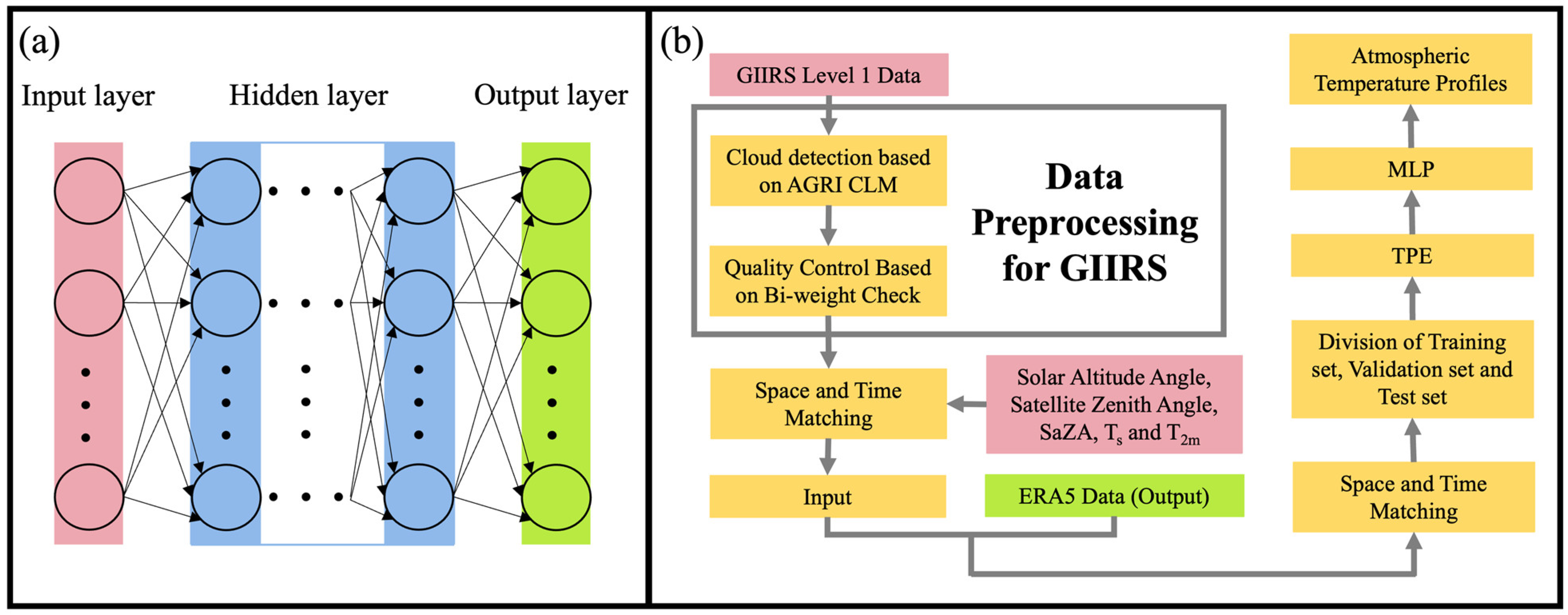
The MLP model includes an input layer, one or more hidden layers, and an output layer, as shown in Figure 2a.
The output of the input layer and hidden layer can be expressed as:
O = f w I + b
where O is the output, I is the output of the previous layer, w is the weight matrix, b is the bias matrix, and f is the activation function. For the input layer, the 689 long-wave infrared channels, solar altitude angle, satellite zenith angle, Ts, and T2m are used as the input nodes. The use of the 1D-Var algorithm for retrieving atmospheric temperature profiles necessitates the careful selection of GIIRS channels to optimize computational efficiency [36]. Nevertheless, machine learning techniques exhibit substantially accelerated retrieval speeds, meeting the demands of practical applications, and utilizing a greater number of channels provides more comprehensive atmospheric information. Consequently, in this research, we employed all available long-wave channels. The inclusion of the solar altitude angle is necessary due to the diurnal variation bias characteristics of GIIRS, and the inclusion of satellite zenith angle is due to a significant correlation between the bias and satellite zenith angle [19]. Additionally, the Ts and T2m are included to provide atmospheric information near the surface, where the satellite detection capabilities are weaker. In the realm of machine learning models, the capacity to incorporate supplementary information for augmenting the model’s input layer is a fundamental advantage. This capability significantly expands the model’s ability to assimilate and process a wide range of data, consequently enhancing the overall efficacy of machine learning models. For the output layer, the ERA5 temperature data of 27 pressure levels which are greater than or equal to 100 hPa are used as output nodes.
The activation function of the hidden layer was selected by TPE. Three commonly used activation functions were used here, namely relu, tanh, and sigmoid. The formulas of the three activation functions are listed in Table 1. The linear activation function was chosen for the output layer. The model optimizer was Adam. Adam combines the advantages of two popular optimization methods: the ability of AdaGrad to deal with sparse gradients and the ability of RMSProp to deal with non-stationary objectives [57]. The mean squared error ( M S E ) is used as the loss function, and its formula is shown as follows:
M S E o , y = i = 1 n o i y i 2 n
where o is the output and y is the target.
(b)
Tree-structured Parzen Estimator (TPE)
TPE is a SMBO algorithm that uses a probabilistic model generated by the Parzen window density estimator. This method divides the initial observations A t 0 into two groups and then adds the multiple Gaussian probability distributions generated at each point to generate the probability density Function (7) for each group.
p x y = l x      i f   y < y * g x      i f   y y *
where l x is the density formed by using the observations { x i } such that corresponding loss f ( x i ) is less than y * and g x is the density formed by using the remaining observations. The TPE algorithm chooses y * to be some quantile γ of the observed y values, so that p y < y * = γ .
Then, c candidates are generated using the probability density function and EI for each sampled point are calculated by the following equation:
E I y * x = y * y * y p x y p y p x d y
After deducing [47], EI can be expressed as:
E I y * x = γ y * l x l x y * p y d y γ l x + 1 γ g x γ + g x l x 1 γ 1
This last expression shows that to maximize improvement, points x with high probability under l ( x ) and low probability under g ( x ) are preferred. The tree-structured form of l and g makes it easy to draw many candidates according to l and evaluate them according to g ( x ) / l ( x ) . The hyper-parameter set x * showing the maximum EI is evaluated through the actual model and is included in the next observation set A t for modeling. Thereafter, the process of updating the model and finding the optimal point is repeated, as described in Algorithm 1. Note that a few iterations of random searching are necessary to warm up the TPE algorithm.
The objective of this study was to minimize the deviation between the retrieved temperature and ERA5. To achieve this goal, f ( x ) is defined as the average RMSE of all pressure levels in the test set:
f x = h = 1 H ( n = 1 N X n h Y n h 2 N ) H
where X n h represents the retrieval results, Y n h represents the temperature of ERA5, N represents the total number of sample pairs, and H represents the number of pressure levels.
Algorithm 1. Tree-structured Parzen Estimator (TPE)
1: Generate i   observations   A i = { x i ,     f ( x i ) } by random searching.
2: While i < i m a x do
3: Divide A t   into   two   groups   based   on   y *
4: Compute l x   and   g x by adding the likelihood probability distribution of all points included in each group.
5: Generate several candidates x i c a n d
6: Set x * = a r g m i n { g ( x ) / l ( x ) }
7: Evaluate f x *
8: Update A i + 1 = { A i ( x * , f x * ) }
9: end while
10: Find x b e s t = a r g m i n { f ( x ) }   in   A i m a x
11: Return x b e s t
In this study, the Hyperopt library in Python is used to implement TPE. The recommended values of γ , c , and i were used, which were 0.25, 24, and 20, respectively, and i m a x was set to 100. Six hyper-parameters were optimized, including number of hidden layers, number of neurons in hidden layer, learning rate, patience value, activation function, and batch size (Table 2). It should be noted that “patience” is a parameter in TensorFlow used to control the number of iterations in the MLP model. If the validation loss value does not decrease after the patience value iterations, the iteration process will stop.

2.2.3. Process of TPE-MLP Model

The flowchart of the TPE-MLP model for retrieving the atmospheric temperature profile is illustrated in Figure 2b. The matched data pairs were subjected to clear-sky screening, quality control, and temporal–spatial matching before being divided into training, validation, and test sets. The training set consists of data collected between 2020 and 2021 (approximately 940,000 samples), while the data from 2022 were randomly divided into validation (30%, approximately 160,000 samples) and test (70%, approximately 380,000 samples) sets. It can be seen that the number of samples used for model training is sufficient, and the test set is completely independent of the training set. The hyper-parameters of MLP were then optimized by TPE, and the optimized hyper-parameter values were substituted into MLP to retrieve the atmospheric temperature profiles.

2.2.4. Evaluation Methods

Three statistical metrics are used to assess, quantitatively, the retrieval accuracy of the model, namely RMSE, mean bias (MB), and standard deviation (STD), as expressed below:
R M S E = i = 1 n X i Y i 2 n
M B = i = 1 n X i Y i n
S T D = i = 1 n X i Y i M B 2 n
where X i is retrieved temperature, Y i is the target value, and n is the number of samples.

3. Results

Firstly, five sets of sensitivity experiments were designed to examine the influence of individually incorporating solar altitude angle, satellite zenith angle, Ts, and T2m into the input layer of the MLP model on the retrieval accuracy (Table 3). Subsequently, a comparison was made between the optimization results of the TPE algorithm and the random search algorithm, followed by a comprehensive discussion of the factors that influence the retrieval accuracy, based on a comparison of the retrieved temperature profiles with ERA5 data. Furthermore, to provide a more thorough assessment of the retrieval accuracy, a comparison was conducted between the retrieved temperature profiles and in situ sounding data. To evaluate the model’s generalization ability, the analysis presented in this study focuses primarily on the results obtained from the test set.

3.1. Sensitivity Experiments for the Input Layer

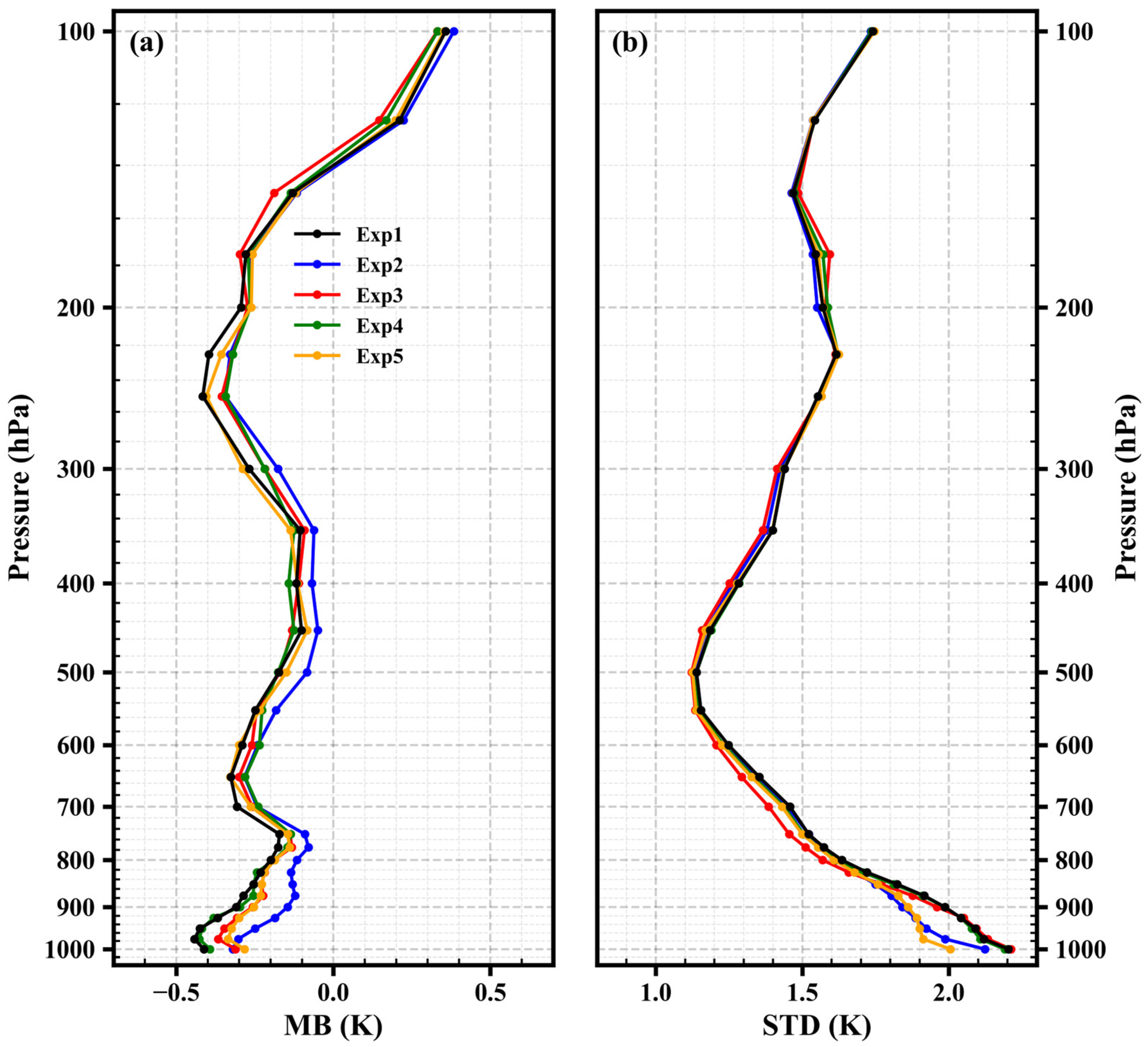
For the five sets of experiments presented in Table 3, each set was conducted 10 times, and the mean bias and standard deviation were calculated for each experiment. Figure 3 illustrates the average mean biases and standard deviations of the 10 retrieval results for each set of experiments. Compared with Exp1, the inclusion of solar altitude angle, satellite zenith angle, Ts, and T2m result in varying degrees of improvement in retrieval accuracy.
Firstly, the average mean biases for each set of experiments range from −0.5 K to 0.5 K. The retrieved temperatures show cold biases compared to ERA5, except for 125 and 100 hPa. Compared to Exp1, the absolute values of mean biases are smaller for Exp2–5 in most pressure levels, particularly in the range of 1000–600 hPa. Notably, the inclusion of solar altitude angle demonstrates the most significant improvement in mean biases, with the minimum absolute values observed in most pressure levels.
The vertical variation of standard deviations for Exp1–5 is depicted in Figure 3b. The average standard deviations for each set of experiments vary from 1.12 to 2.21 K. Adding solar altitude angle to the MLP model’s input layer leads to decreased standard deviations in most pressure levels, particularly in the pressure range of 1000–800 hPa. Compared to Exp1, the average standard deviation of all pressure levels is reduced by approximately 2.54%, with a reduction of about 5.29% in the pressure range of 1000–800 hPa. Similarly, the addition of satellite zenith angle results in a significant reduction in standard deviation in most pressure levels compared to Exp1, with an average reduction of approximately 1.37% of all pressure levels. Unlike solar altitude angle, the reduction in standard deviation due to the addition of satellite zenith angle is observed primarily in the 900–300 hPa range, while in the pressure range of 1000–800 hPa, the addition of solar altitude angle results in more reduction of standard deviation.
It is worth noting that the addition of Ts does not show a significant reduction in standard deviations, except for a slight decrease in the pressure range of 1000–500 hPa. On the other hand, the inclusion of T2m leads to a decrease in standard deviations in the pressure range of 1000–400 hPa, particularly in the pressure range of 1000–850 hPa. Compared to Exp1, the average standard deviation of all pressure levels decreases by approximately 2.95% after the addition of T2m, with a reduction of about 7.24% in the pressure range of 1000–850 hPa. Notably, the inclusion of T2m contributes the most to the reduction of standard deviations in the pressure range of 1000–925 hPa.
As mentioned earlier, the addition of Ts does not have a significant effect on the reduction of standard deviations, primarily for the following reasons: (1) the issue of representativeness in observations, as the GIIRS footpoint is around 16 km and Ts observations characterize only a small area, leading to discrepancies between observed Ts and actual Ts at the GIIRS observation location; and (2) the sparse Ts observations (Figure 1b), which introduce errors in the interpolation. Additionally, surface radiation, although being a very important part of the radiation received by satellites, does not seem to learn this physical process in the MLP model. However, despite these limitations, the inclusion of Ts reduces the absolute value of mean biases and results in a slight decrease in standard deviations in the pressure range of 1000–500 hPa, hence Ts is still utilized as the input node in the MLP model for the subsequent retrieval process.

3.2. Hyper-Parameter Optimization

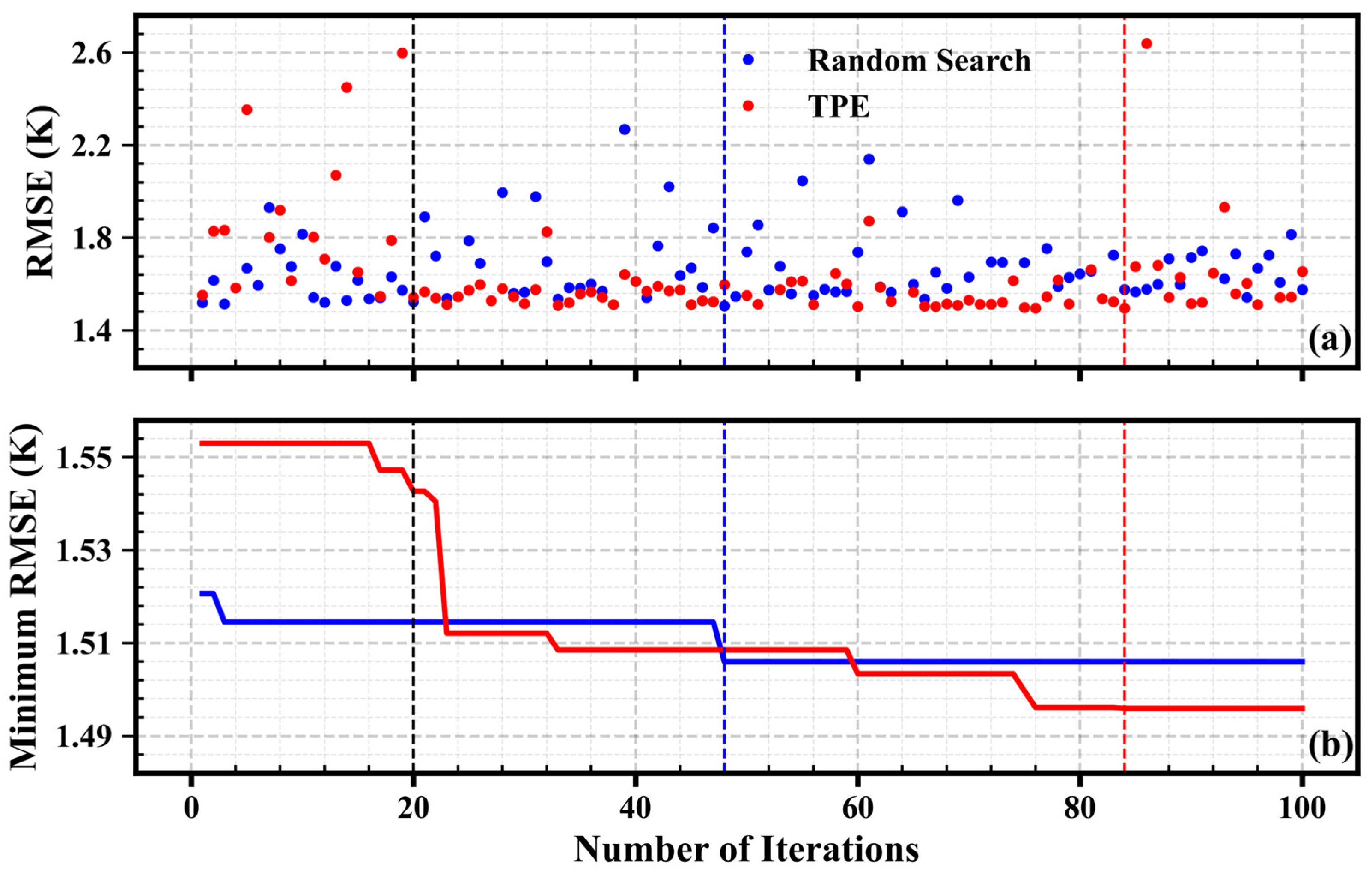
In this study, the TPE algorithm was used to optimize the hyper-parameters of MLP. The advantages of the TPE algorithm are highlighted by comparing its optimization results with those obtained from the random search method. One hundred hyper-parameter searches were conducted using both the random search method and the TPE algorithm. As described in Section 3.2, the first 20 iterations of the TPE algorithm utilized the random search method. Figure 4 shows the variation in average RMSEs with the number of iterations for the two methods. During the first 20 iterations, the average RMSE values for both the TPE experiment and the random search experiment were quite scattered, ranging primarily from 1.5 K to 2.0 K. In the following 80 iterations, the TPE algorithm showed a significant advantage. Compared to the random search method, the TPE algorithm’s average RMSE values were smaller in most of the iteration steps and had a narrower range of variation. In the TPE algorithm, 68.75% of the iteration steps had an average RMSE lower than 1.7 K, while in the random search method, only 37.5% of the iteration steps achieved an average RMSE below 1.7 K.
Figure 4b shows the variation of the minimum RMSE with the number of iterations. The minimum RMSE represents the lowest value of the average RMSE obtained in the completed iterations. For the first 20 iterations, the random search experiment quickly identified a set of better parameters, resulting in a small RMSE value. In contrast, although the TPE algorithm also adopted the random search method in the initial 20 iterations, it resulted in larger RMSE values. This also indicates that the random search method depends only on random probability. In the following 80 iterations, the minimum RMSE of the random search method was only updated in the 48th iteration step. During the iteration process of the TPE algorithm, the minimum RMSE rapidly declined, dropping to levels below that of the random search method, and continued to decrease in subsequent iterations. Ultimately, the TPE algorithm achieved better results than the random search method. The optimal parameters obtained by the TPE algorithm are shown in Table 4.
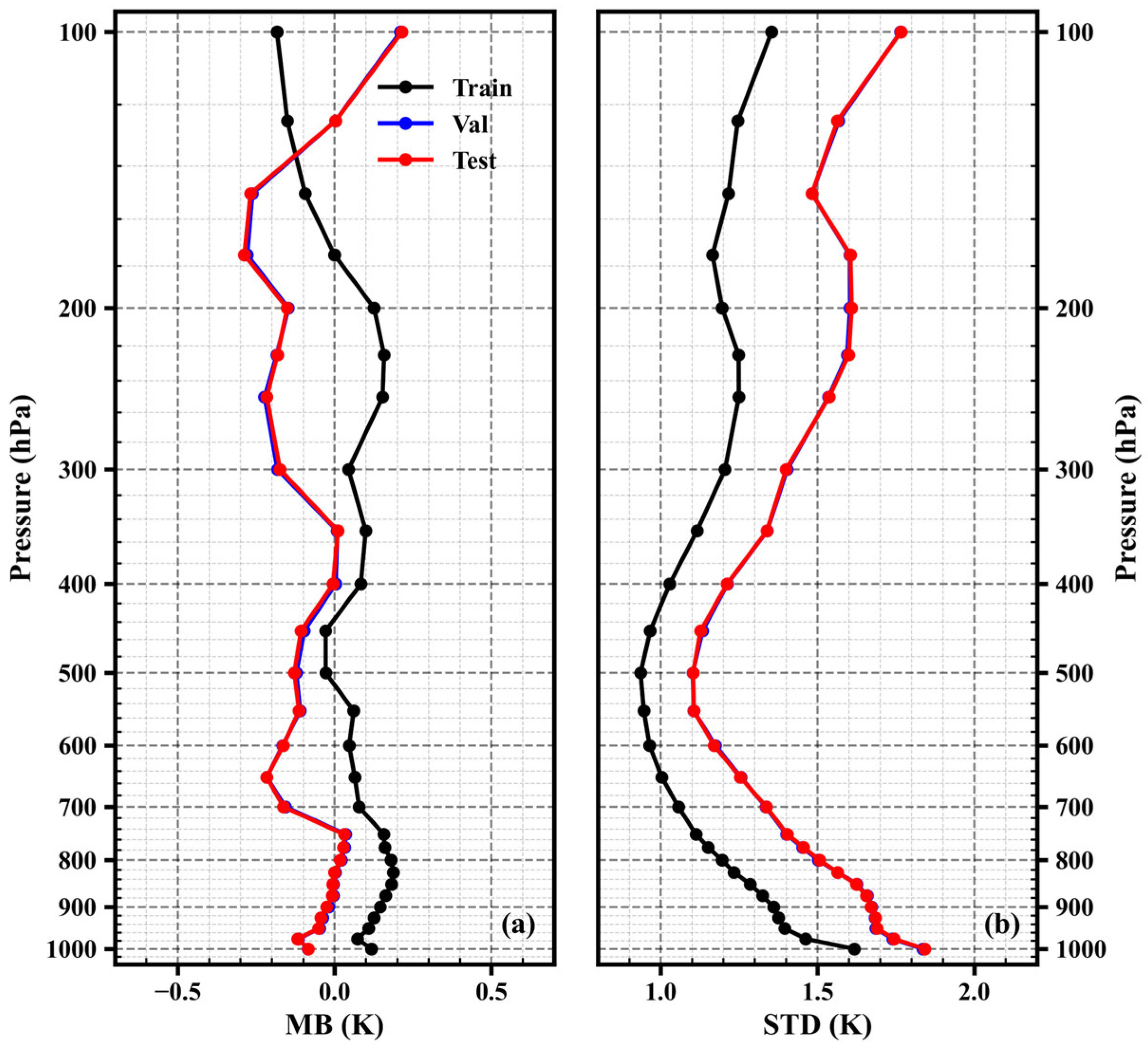
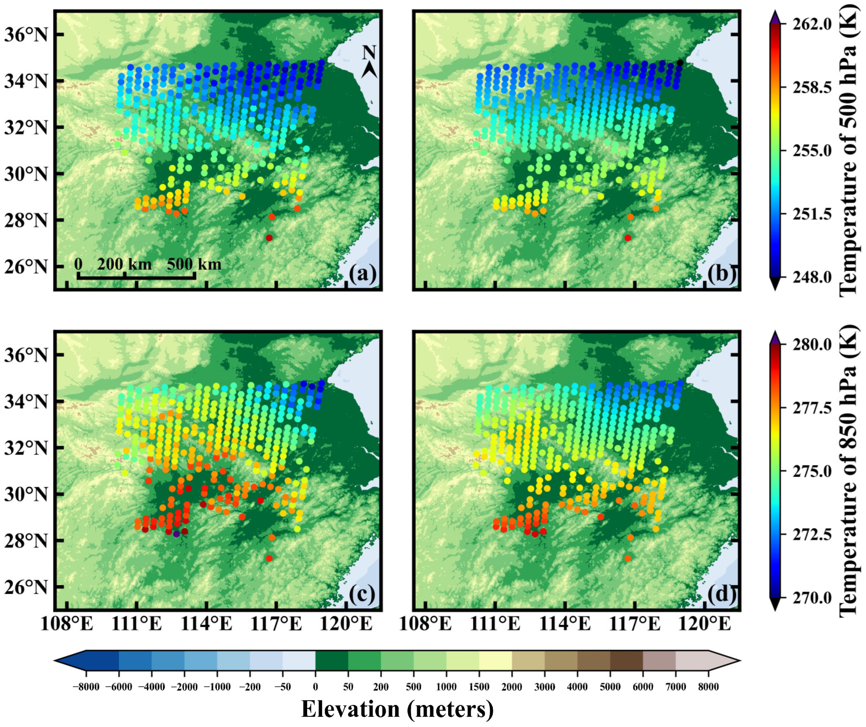
Figure 5 shows a comparison between the temperature profiles retrieved using the optimized hyper-parameters and the ERA5 data. The mean biases of the training set are close to 0 for different pressure levels, and the standard deviations vary from 0.94 K to 1.62 K for different pressure levels, with a minimum value occurring at 500 hPa. Since both the validation set and test set were randomly selected from the data of 2022, their results are similar. Similar to the results in Figure 3a, the retrieved temperature profiles of the test set exhibit mainly cold biases, with mean biases ranging from −0.36 K to 0.23 K. The negative bias exhibited by the test set compared to the training set may be related to changes in the instrument’s detection performance. The maximum absolute value of the bias occurs at 650 hPa, while the minimum absolute value occurs at 450 hPa. The standard deviations range from 1.10 K to 1.84 K for different pressure levels, with the maximum value occurring at 1000 hPa and the minimum value occurring at 500 hPa. Figure 6 displays the horizontal distribution of retrieved temperatures compared to the corresponding ERA5 temperatures at 20:00 on 2 January 2022. As shown, the retrieval results closely align with ERA5, particularly at 500 hPa.

3.3. Analysis of Influencing Factors

3.3.1. Variation with Detectors

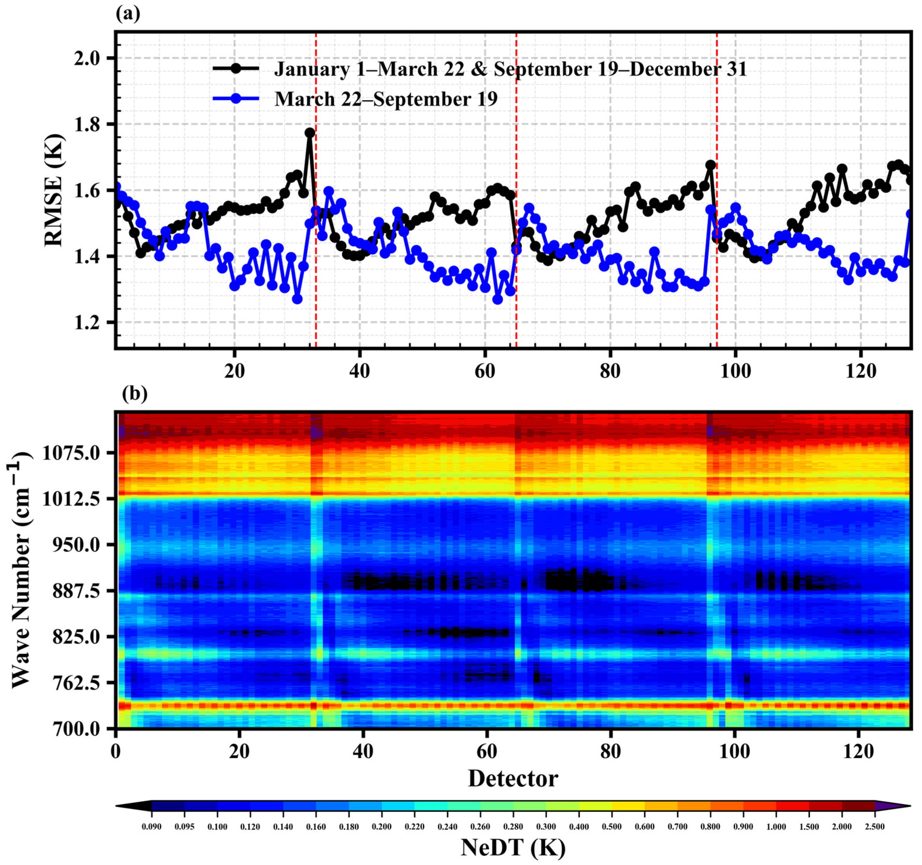
GIIRS comprises a 32 × 4 array of detectors. As described in Section 2, the scanning direction of GIIRS changes around the spring and autumn equinoxes. For ease of discussion and analysis, the results are divided into two time periods for separate discussion based on the timing of the north–south orbit control and the pointing adjustment of the satellite radiation cooling screen. The first time period spans from 1 January to 22 March and 19 September to 31 December and the second time period spans from 22 March to 19 September.
Figure 7a illustrates the variation of the average RMSEs of all pressure levels with detectors. The RMSEs of the 128 detectors for the first time period spans range from 1.39 K to 1.77 K, while the RMSEs for the second time period spans are smaller, varying from 1.27 K to 1.61 K. The reason for the different results for the two time period spans is similar to the monthly variation, which will be discussed in Section 3.3.2. The results for both time periods show that the RMSEs are smaller near the center of each column (32 detectors) and larger on the north and south sides. Additionally, the distribution of RMSEs for each column of detectors is not symmetrical. In both time periods, there are more detectors with larger RMSEs on the north side, while the detector with the minimum RMSE is located near the south side (the scanning pattern is described in Section 3.1). Figure 7b displays the average NeDT (noise equivalent delta temperature, NEΔT) for 128 detectors for the second time period (the results for the first time period are similar, Figure S1). For the upper tropospheric channels (channels 2–20 or 700.625–711.875 cm−1), middle tropospheric channels (channels 21–30 or 712.5–718.125 cm−1), and lower tropospheric channels (channels 71–90 or 743.75–755.625 cm−1) [19], the NeDT for each column of detectors exhibits larger values on both sides and smaller values near the center of each column, with the detector having the smallest NeDT located near the side with the smaller numbering (for example, among detectors 1–32, the detector with the smallest NeDT is near the detector numbered 1, rather than the detector numbered 32). For the first time period, the distribution of NeDT is consistent with the changes in RMSEs, but in the second time period, they are inconsistent. The larger RMSEs on both sides of each column are influenced by NeDT, but the north–south differences in RMSE are influenced mainly by other factors.
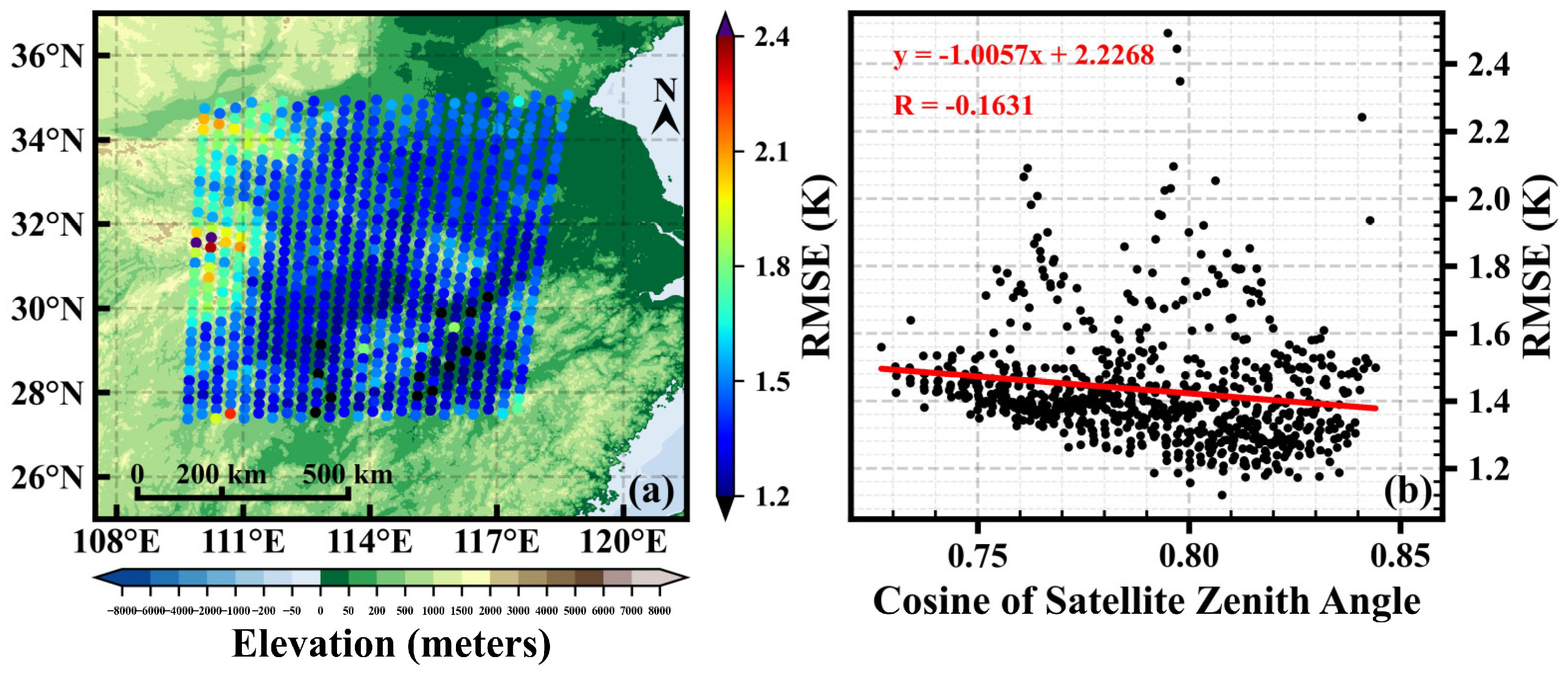
Figure 8a shows the distribution of the average RMSEs with the position of scan sites for the second time period spans. The average RMSEs are significantly influenced by terrain. The scan sites with large RMSEs are mainly concentrated in high elevation areas, where the terrain is relatively complex, and the complex terrain makes it difficult for the algorithm to retrieve the profile with high accuracy [39]. Certainly, the terrain differences exhibited in the results may also be related to training and comparison on isobaric surfaces. For high-terrain areas, some pressure levels are located underground, and the retrieval of these pressure levels may result in larger RMSEs. In this paper, these factors are collectively considered as terrain influence. High elevation areas are mainly located in the northwest of the study area, which is one of the reasons for the large RMSE on the north side. The 14th scan site in the first scan line (from north to south) is also located at a high elevation and has a large RMSE, which corresponds to the larger RMSE observed for the 14th detector in Figure 7a.
In addition to the influence of terrain, we also found a significant correlation between the average RMSEs and the cosine of satellite zenith angles, with a correlation coefficient of approximately −0.16 (Figure 8b, the points with large RMSE are mainly caused by terrain). As shown by the red fitted line, there is a significant negative correlation between the average RMSEs and the cosine of satellite zenith angles. Geostationary satellites have non-vertical satellite zenith angles, which causes the temperature gradient in the slant path to be non-negligible. The greater the satellite zenith angle, the longer the slant path at the same height, and the larger the brightness temperature deviation. The sub-satellite point of FY-4A geostationary satellite is located at 104.7°E, and the study area is situated to the northeast of the sub-satellite point of FY-4A. For a certain scan line, the satellite zenith angle at the northern scan site is greater than that at the southern scan site, which is the second reason for the larger RMSEs of the northern detectors.
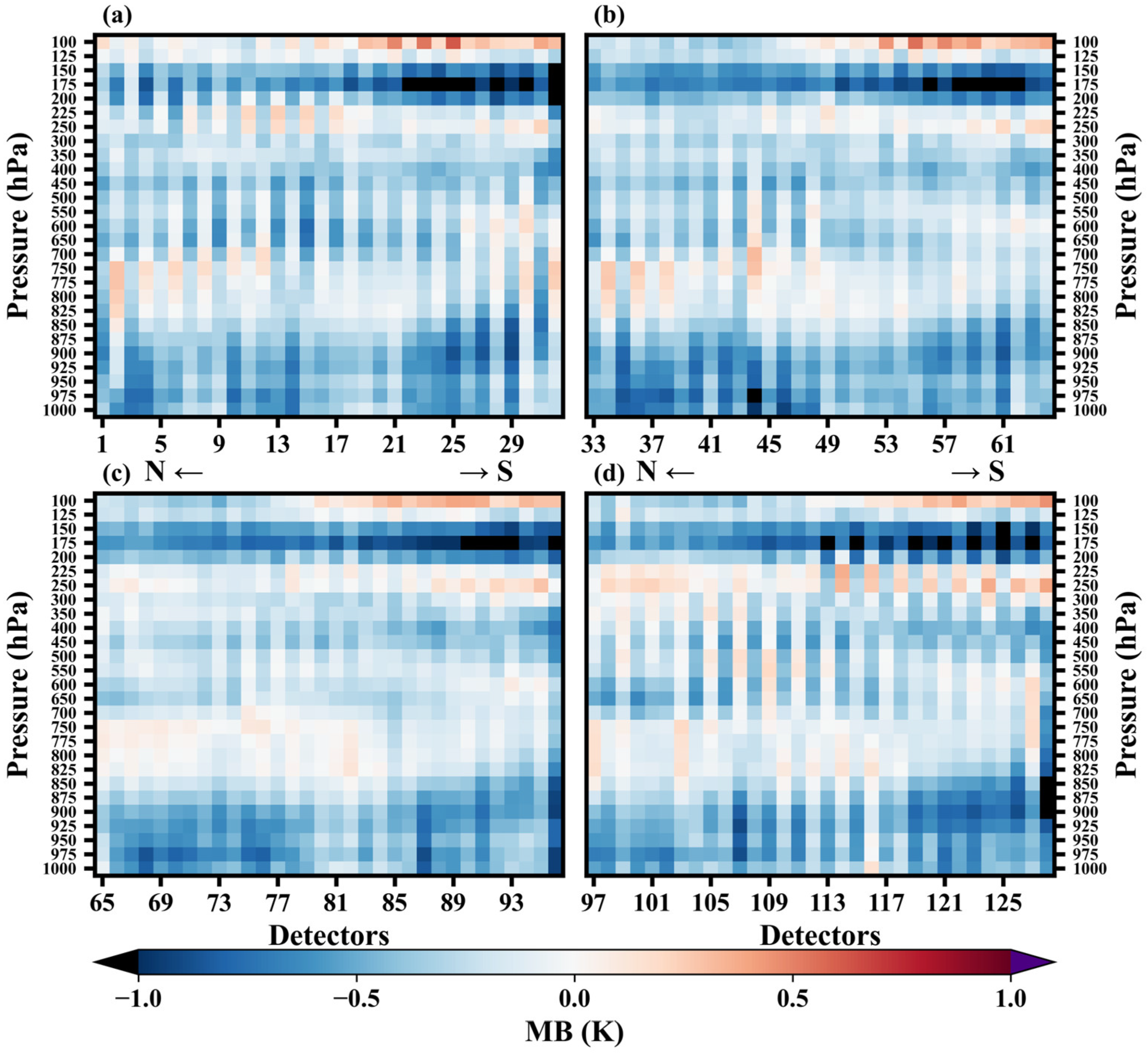
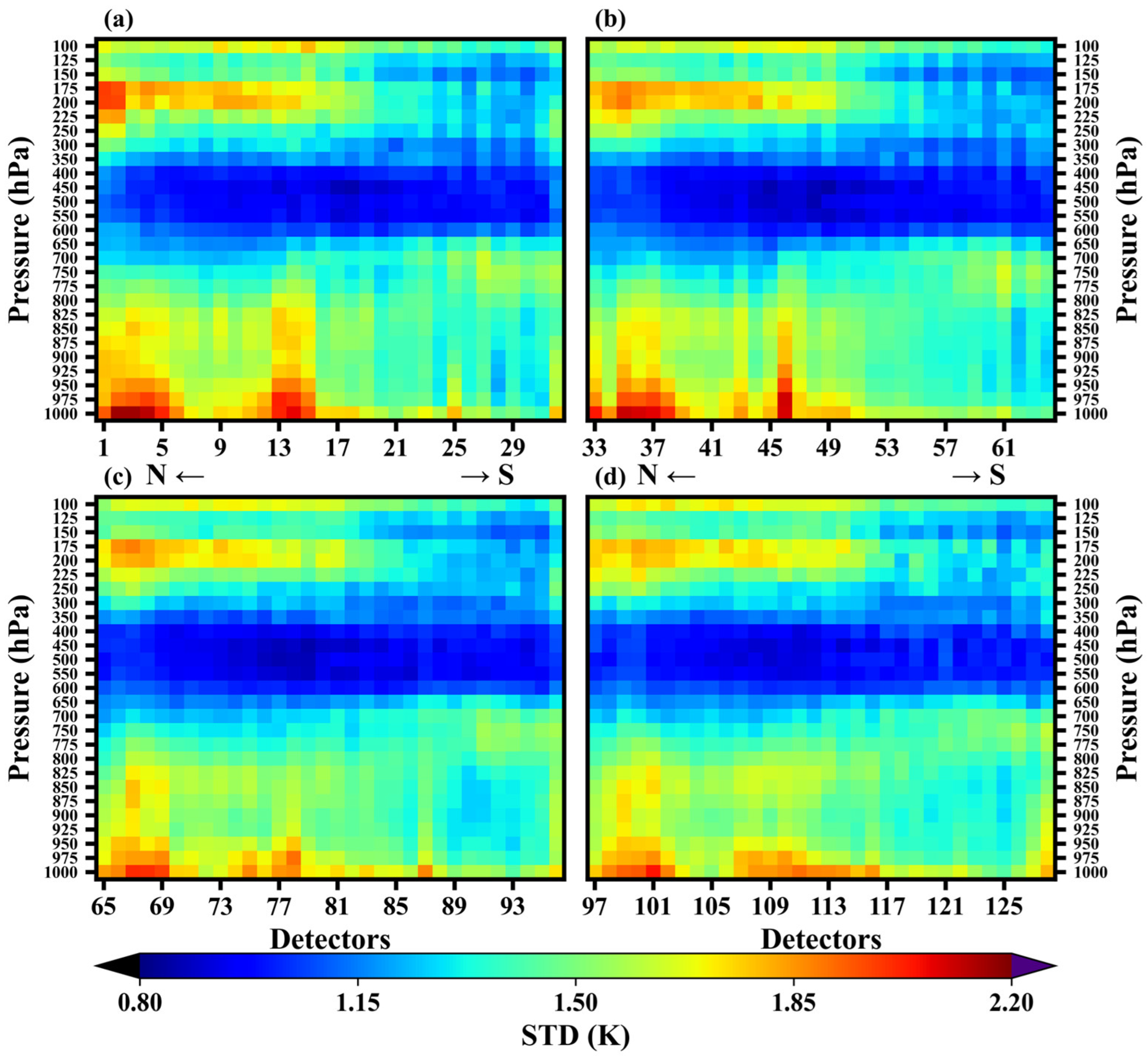
Figure 9 illustrates the variation of mean biases with detectors for different pressure levels. The mean biases are mainly between −1 and 1 K. It is noteworthy that the mean biases of the two adjacent detectors show significant differences, which is caused by the fact that different circuit boards are used for detectors corresponding to odd and even serial numbers, respectively. But for the third column of detectors (Figure 9c), this phenomenon is not as pronounced as for the other columns. In the pressure range of 1000–875 hPa, all detectors, except for detector 116, exhibit cold biases. These cold biases are smaller for central detectors, such as detectors 17–21 and 80–85. In the pressure range of 850–750 hPa, the biases of the individual detectors are generally small. However, some of the detectors on the north and south sides show significant cold biases. In the pressure range of 700–300 hPa, most detectors show cold biases, and there are significant differences between adjacent detectors. In the pressure range of 250–100 hPa, mean biases are influenced by the slant path, showing a significant north–south difference. For the pressure levels of 250, 225, 125, and 100 hPa, the mean biases show a shift from negative to positive biases from north to south. For the pressure levels of 200, 175, and 150 hPa, most detectors show cold biases and the absolute value of mean biases become larger from north to south. The north–south differences of mean biases for the 250–100 hPa during the first period exhibit similar characteristics (Figure S2). In this study, satellite zenith angle was used as an input node, but the biases caused by the slant path do not seem to be fully resolved.
Figure 10 shows the variation of standard deviations with detectors for different pressure levels, ranging from 0.85 K to 2.16 K. In the pressure range of 1000–750 hPa, the standard deviations are larger on the north side, and are mainly influenced by terrain. Similar to the results in Figure 7a, for example, the STD is larger near the 14th detector. The standard deviations of the southern detectors are smaller, but the area with minimum value is not at the southern end, but south of the center. In the pressure range of 700–300 hPa, the standard deviations are relatively small compared to other pressure levels, and they are larger on the north and south sides and smaller near the center. Based on the NeDT of different detectors in the middle troposphere (Figure 7b), detectors located on the southern side should exhibit a smaller standard deviation compared to the northern side. However, the results do not show this phenomenon, which may be due to interference from other channels in the retrieval process, as well as the combined effects of terrain and satellite zenith angle. In the pressure range of 250–100 hPa, the standard deviations decrease significantly from north to south. This is mainly due to the slant path. For a certain scan site, there is a position deviation in horizontal direction due to the slant path, and position deviation increases with increasing altitude. Therefore, the effect of the slant path is more significant at higher altitude. The first time period exhibits similar results (Figure S3).
Based on the results presented above, it can be seen that the retrieval accuracy of the lower troposphere is influenced primarily by terrain, the middle troposphere is affected by a combination of factors, and the upper troposphere is mainly influenced by satellite zenith angle.

3.3.2. Monthly Variation

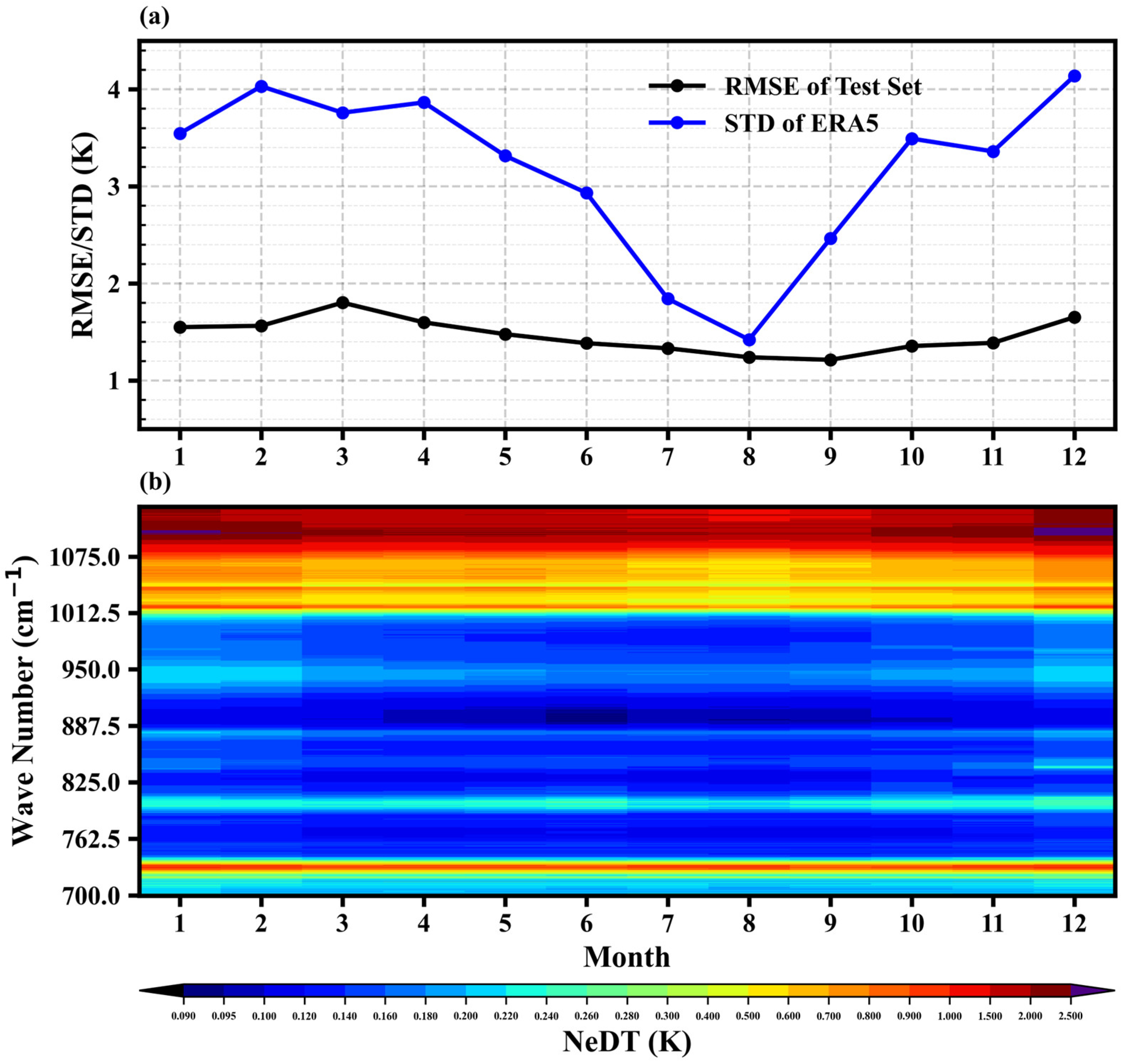
The monthly variation of the average RMSEs of the test set is presented as a black line in Figure 11a. The average RMSEs of the test set range from 1.21 K to 1.80 K, with an increasing trend from January to March, a decreasing trend from March to September, and an increasing trend from September to December [58]. Observational noise is a major factor affecting the accuracy of the retrieval results. Figure 10b displays the monthly variation of the average NeDT corresponding to the test set samples. GIIRS observations have better signal-to-noise ratio in summer than in winter, and most channels exhibit the lowest levels of noise in August. In addition, the monthly variation characteristics of the average RMSEs are related to the horizontal temperature gradient. The horizontal temperature gradient in winter is larger than in summer, leading to greater temperature differences between different profiles in winter, which increases the uncertainty in the retrieval results. The blue line in Figure 10a shows the monthly variation of the average standard deviations of all pressure levels of ERA5 temperature matched to the test set. The trend of average RMSEs is consistent with the variation of the average standard deviation. It should be noted that the statistical RMSEs are also related to the distribution of observational data. As shown in Figure 11a, the average standard deviation and NeDT in March are smaller than in February, but the RMSE is larger in March. This is because there are more clear observations distributed in high-terrain areas in March (Figure S4, located in the northwest).
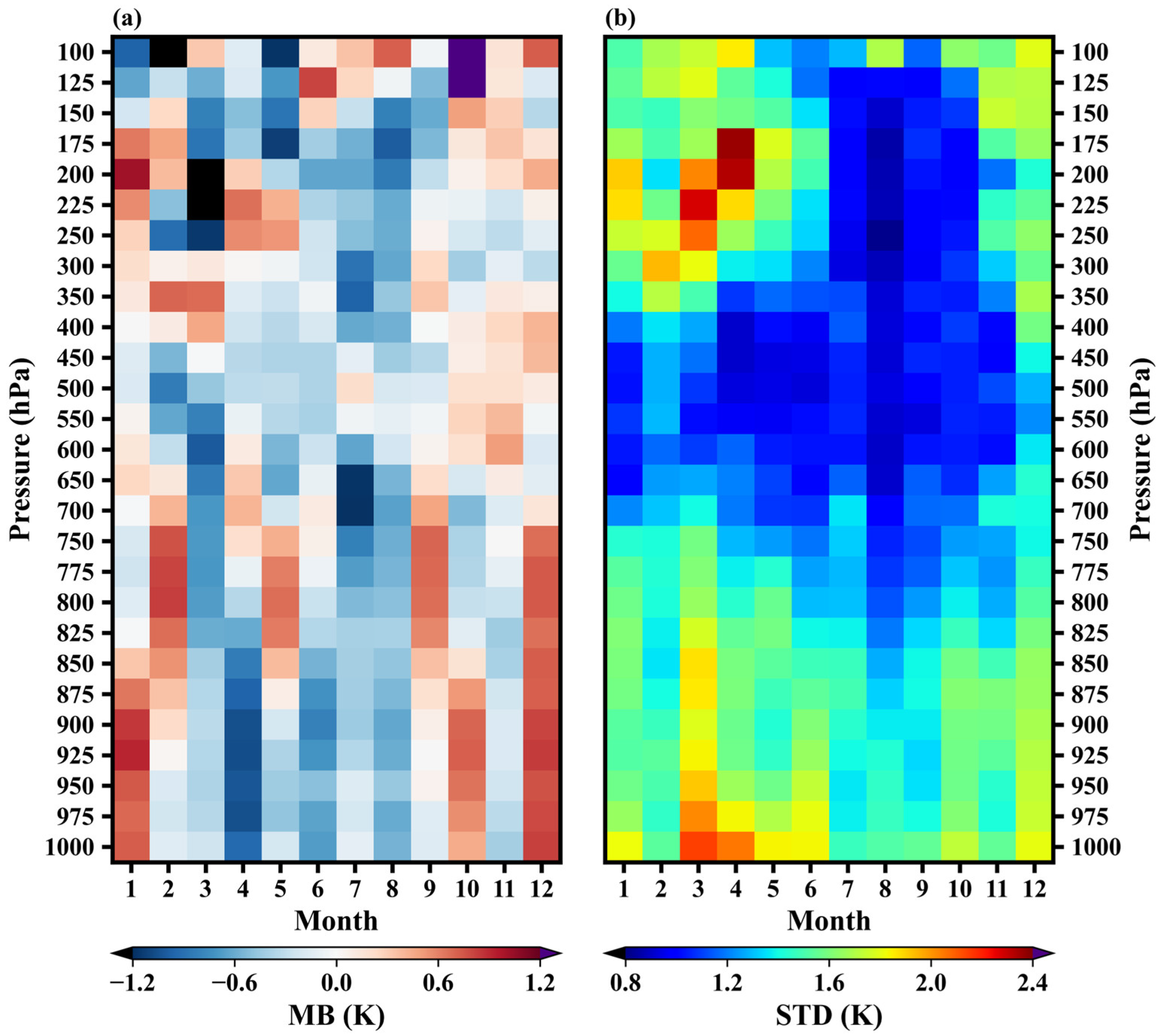
Figure 12 illustrates the monthly variation of mean biases and standard deviations for different pressure levels of the test set. The mean biases range from −1.46 K to 1.48 K. There are more negative biases in summer and more positive biases in winter. The negative biases in summer may be related to higher humidity in summer. The higher the humidity, the lower the observed brightness temperature in humidity-sensitive channels [5]. In the actual retrieval process, machine learning methods struggle to distinguish between temperature and humidity channels. This leads to a bias in the learning results towards interpreting higher brightness temperatures as higher temperatures, as this is easier to learn. However, the observed brightness temperature in humidity-sensitive channels is lower in summer, resulting in lower retrieved temperatures. Of course, further research into the physical interpretation of these machine learning methods is needed, and we will explore this in the future. In the pressure range of 1000–875 hPa, the retrieved temperatures show significant warm biases in January, October, and December, and mainly cold biases in the other months. In the pressure range of 850–700 hPa, February, May, September, and December are dominated by positive biases, while other months are dominated by negative biases. In the pressure range of 650–450 hPa, the retrieved temperatures show mainly cold biases from February to September, and mainly warm biases in other months. In the pressure range of 400–300 hPa, the retrieved temperatures show mainly cold biases from April to August. In the pressure range of 250–100 hPa, negative biases are mostly observed from March to September, while positive biases dominate the remaining months.
The standard deviations range from 0.82 K to 2.36 K. For almost all pressure levels, the standard deviations show an up-down-up trend from January to December, excluding the February results. In February, the standard deviations are smaller than in January and March at some pressure levels, mainly concentrated in the lower troposphere. This is due to the distribution of the data (Figure S4). In the pressure range of 1000–750 hPa, standard deviation reaches maximum value in March and the minimum values occur in July, August, or September. In the pressure range of 700–550 hPa, standard deviation reaches maximum value in December and minimum value in August. In the pressure range of 500–400 hPa, standard deviation reaches its maximum value in December and minimum value in April. In the pressure range of 350–100 hPa, the maximum value of standard deviations occurs in February, March, or April, while the minimum value of standard deviations occurs mainly in August or September. The distribution of the standard deviation is related to the height of the tropopause. Temperature retrievals in the vicinity of the tropopause tend to be less accurate due to the minimal change in temperature with height [59,60]. From winter to summer, due to the increase in solar radiation, the height of the tropopause rises, resulting in a higher altitude of the region with larger standard deviations.

3.3.3. Diurnal Variation

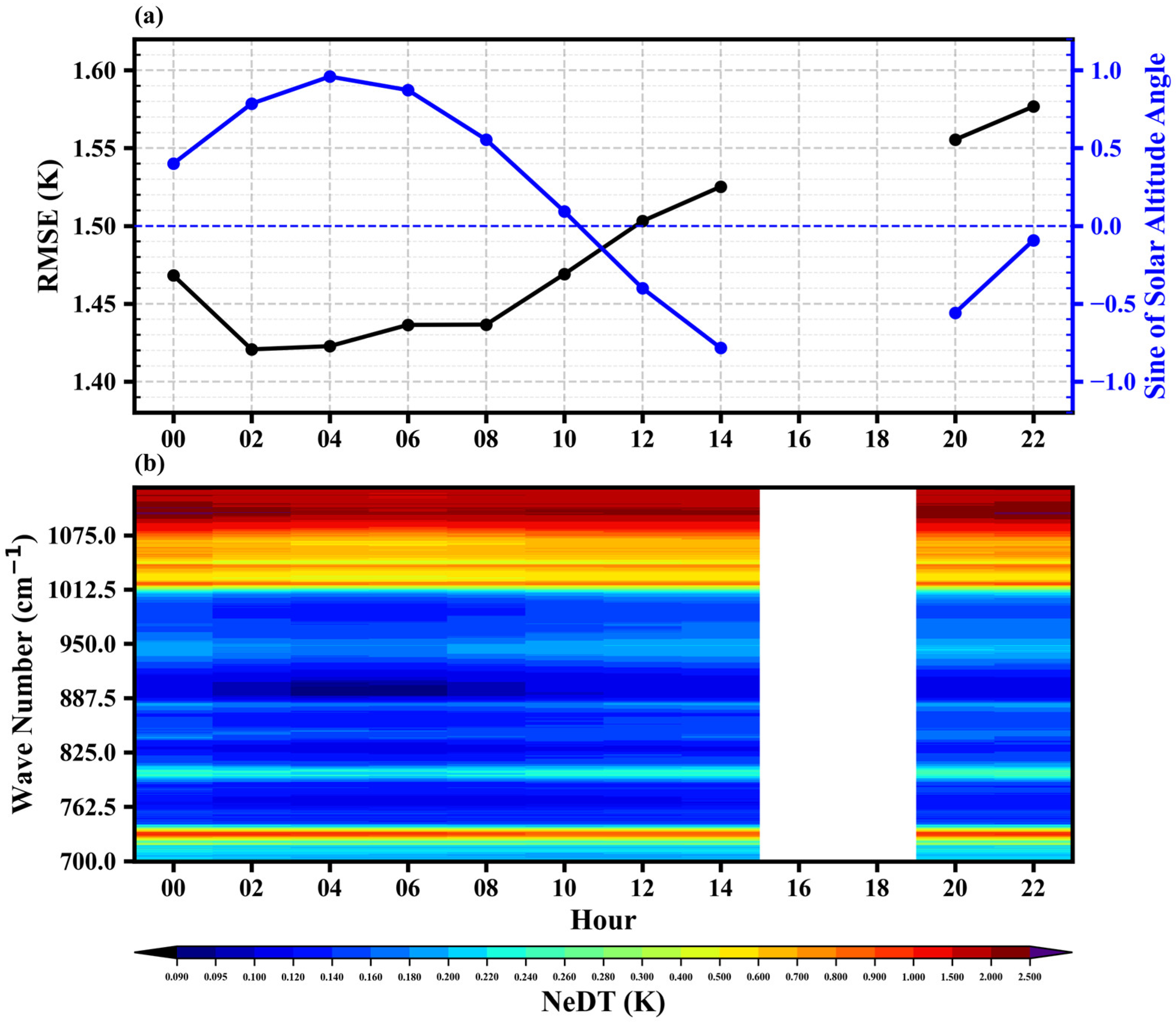
The GIIRS, orbiting in geostationary orbit, is affected by solar radiation, and the diurnal variation bias between observations and simulations is obvious [19]. Figure 13a illustrates the diurnal variation of the average RMSE of the test set, which varies from 1.42 to 1.58 K. It is important to note that the thermal environment of instruments on geostationary satellites is easily affected by solar radiation, hence GIIRS does not conduct observations from 16:00 to 18:00 UTC each day. From 00:00 to 22:00, the RMSE shows a decreasing trend followed by an increasing trend. The diurnal variation characteristic of the average RMSE is similar to the diurnal variation characteristic of the bias between observations and simulations found by Yin et al. [19]. Due to the diurnal variation of solar altitude angle, the GIIRS is affected by the solar radiation to different degrees at different moments. As shown in Figure 13, when the solar altitude angle is positive, the sun is at the back of the instrument, and the instrument is less affected by solar radiation. The average RMSEs are small at those moments (From 00:00 to 10:00). When the solar altitude angle is negative, the sun is in front of the instrument, and the instrument is more affected by solar radiation. The average RMSEs are large at those moments (From 12:00 to 22:00). NeDT also shows significant diurnal variation due to solar radiation and shows a minimum around 04:00 (Figure 13b).
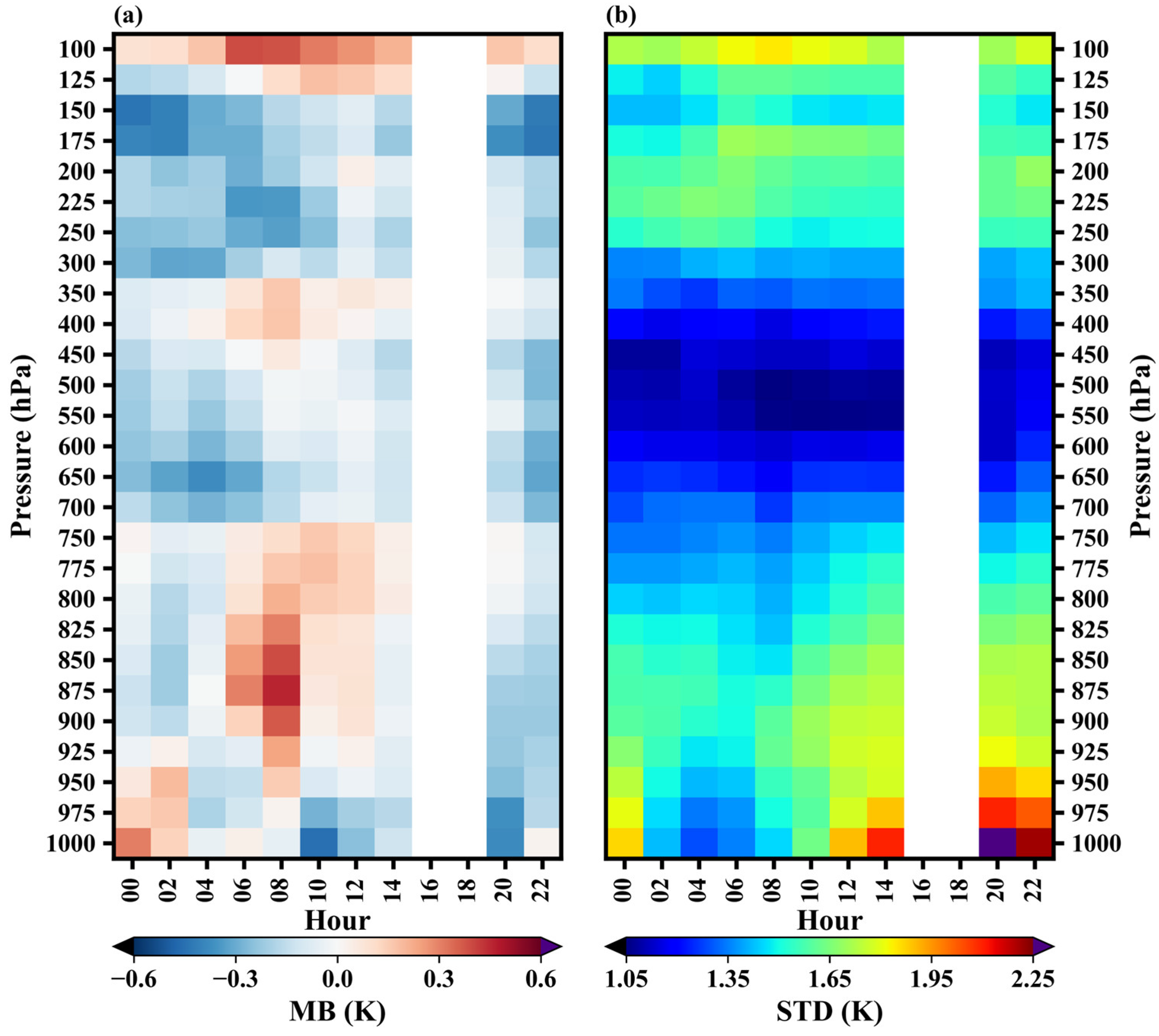
The diurnal variations of mean biases and standard deviations for different pressure levels are shown in Figure 14. The mean biases range from −0.45 K to 0.46 K and exhibit noticeable diurnal variation. In the pressure range of 1000–950 hPa, the mean biases display a transition from positive to negative values. The maximum value is observed at 00:00, while the minimum value occurs at 20:00. In the pressure range of 925–100 hPa, the mean biases exhibit a distinctive pattern of initially increasing and then decreasing, which is consistent with the diurnal variation of the GIIRS bias found by Yin et al. [19]. The largest values of mean biases are observed primarily between 08:00 and 12:00, with a larger number of pressure levels reaching their peak at 08:00. As mentioned above, solar altitude angle is used as an input node. It appears that taking the solar altitude angle as an input node does not completely eliminate the diurnal variation of biases.
The standard deviations range from 1.05 K to 2.31 K and exhibit significant diurnal variation for all pressure levels. In the pressure range of 1000–900 hPa, the diurnal variation of STD is particularly pronounced, following a pattern of decreasing, then increasing, and then decreasing again. The minimum value is observed at 4:00, while the maximum value occurs at 20:00. In the pressure range of 900–350 hPa, the standard deviations display a similar diurnal characteristic to those of 1000–900 hPa. The minimum value is observed at 08:00, and the maximum value is observed at 22:00. The diurnal variation of the standard deviation in the 1000–350 hPa pressure range is influenced mainly by the solar altitude angle and the NeDT. However, in the pressure range of 300–100 hPa, the diurnal variation is less pronounced compared to other pressure levels. Contrary to the trend observed in other pressure ranges, the standard deviations in this range exhibit an increasing trend followed by a decreasing trend. The maximum value is typically reached around 06:00. With increasing altitude, the diurnal variation of STD gradually becomes less pronounced, due to the different intensities of diurnal variation in NeDT across different channels. Some channels near the window (around 900 cm−1) exhibit an obvious diurnal variation in NeDT, while the diurnal variation intensity of NeDT for the upper tropospheric channels (channels 2–20 or 700.625–711.875 cm−1) is weaker (Figure 13b).

3.4. Comparison between Retrieved Temperature Profiles and In Situ Sounding Data

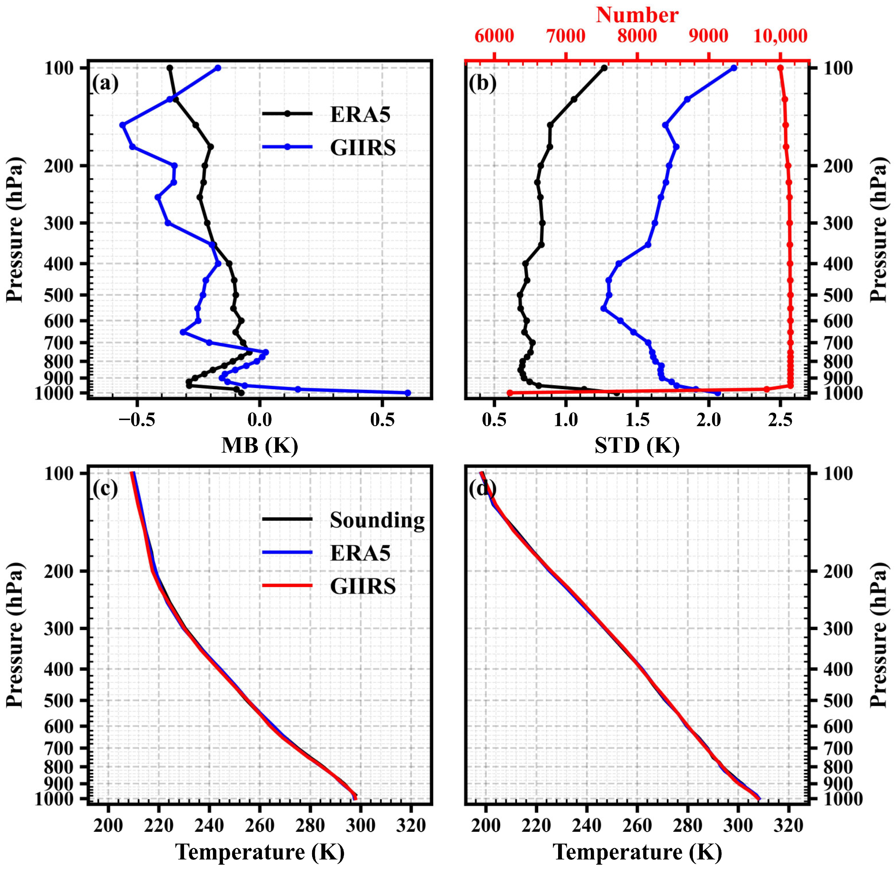
Figure 15a,b shows the mean biases and standard deviations between the ERA5 data and in situ sounding data, as well as the mean biases and standard deviations between the retrieval temperature profiles of the test set and sounding data. As shown by the red line in Figure 15b, there are a total of 10,142 pairs of matched profiles. Some pressure levels have relatively fewer sounding observations, especially at lower levels. Compared to sounding data, ERA5 data show cold biases, with the mean biases ranging from −0.37 K to −0.04 K. The standard deviations vary from 0.68 K to 1.36 K, with values below 1 K in the pressure range of 950–150 hPa. Overall, the ERA5 temperature data demonstrate sufficient accuracy, especially in the pressure range of 950–150 hPa. The strong agreement between RAOBs and ERA5 is partly attributed to the fact that ERA5 has assimilated most available observations including RAOBs, which means the comparisons between ERA5 and RAOBs might not be independent.
The blue line in Figure 15a,b represents the comparison between the retrieved temperature profiles of the test set and in situ sounding data. Similar to ERA5, the retrieval results show cold biases, except for 1000, 975, 775, and 750 hPa. The mean biases range from −0.56 K to 0.60 K, with the maximum absolute value occurring at 1000 hPa and the minimum absolute value occurring at 775 hPa. The standard deviations vary from 1.26 K to 2.17 K, with the maximum value occurring at 100 hPa and the minimum value occurring at 550 hPa. The standard deviations are generally below 2 K, except at 1000 and 100 hPa, and below 1.5 K in the pressure range of 650–400 hPa.
Figure 15c,d presents two examples of comparisons between sounding profiles, ERA5 profiles, and retrieved profiles. The retrieved profile in Figure 15c is located at 112.85°E, 33.05°N on 3 May 2022, at 12:00 UTC, while the retrieved profile in Figure 15d is located at 114.02°E, 30.67°N on 12 August 2022, at 12:00 UTC. As shown in the figure, the three types of profiles exhibit good consistency, further demonstrating the reliability of the retrieved profiles.

4. Discussion

In this study, atmospheric temperature profiles are retrieved based on the TPE-MLP model, using FY-4A/GIIRS long-wave data, with ERA5 data as label data for training. For the input layer of MLP, the 689 long-wave infrared channels, solar altitude angle, satellite zenith angle, Ts, and T2m are used as the input nodes. By incorporating solar altitude angle, satellite zenith angle, Ts, and T2m into the input layer of the MLP model, the retrieval accuracy can be significantly improved. Note that some of those additional parameters, especially the solar angle information, are usually not included in the optimal estimation method. The ability to combine multiple sources of data for retrieving atmospheric temperature profiles is one of the advantages of machine learning models. TPE is more effective than the random search method in optimizing the hyper-parameters of MLP. The set of optimized hyper-parameters obtained through iterative optimization in this study can provide references for future research on using MLP models for retrieving atmospheric temperature profiles.
Comparing the retrieved temperature profiles with ERA5 data, several factors can be seen to affect the retrieval accuracy, including the detector, signal-to-noise ratio, terrain, solar altitude angle, satellite zenith angle, and the horizontal temperature gradient. Detectors located closer to the center of each column have smaller average RMSEs, while those located on the north and south sides have larger average RMSEs. Areas with high terrain and larger satellite zenith angles also exhibit larger average RMSEs. Mean biases of the two adjacent detectors show significant differences for different pressure levels. The retrieval accuracy of the lower troposphere is mainly affected by terrain, the middle troposphere is affected by a combination of factors, and the upper troposphere is mainly affected by satellite zenith angle. Monthly variations in the horizontal temperature gradient and signal-to-noise ratio contribute to a pattern of increasing, decreasing, and then increasing again in the average RMSEs. Mean biases also exhibit variations across different months and pressure levels, and standard deviations demonstrate similar patterns of change in the average RMSEs. The diurnal variation of solar altitude angle and signal-to-noise ratio leads to an obvious diurnal variation in retrieval accuracy, and the intensity of the diurnal variation weakens with altitude increases. Finally, compared to in situ sounding data, the mean biases vary from −0.56 K to 0.60 K and the standard deviations range from 1.26 K to 2.17 K.
The results show that the TPE-MLP model proposed in this paper achieves satisfactory accuracy in retrieving atmospheric temperature profiles from GIIRS hyperspectral IR sounder data. Retrieving atmospheric parameters from GeoHIS observations is of significant value for severe weather situation awareness and nowcasting applications. Furthermore, the analysis of factors influencing the retrieval accuracy provides valuable references for improving the retrieval performance and the practical application of retrieval data in future research. It is recommended to apply bias correction techniques to GIIRS data prior to retrieval, including FOR bias correction, correction for biases in odd and even detectors, and correction for diurnal variation. Furthermore, it is important to account for seasonal and terrain variations during the retrieval process. With its high temporal resolution, GIIRS can provide continuous observation data for the same area and is well-suited for convective monitoring studies. This is one of the research directions we plan to pursue in the future.

Supplementary Materials

The following supporting information can be downloaded at: https://www.mdpi.com/article/10.3390/rs16111976/s1, Figure S1: Average NeDT of each channel for 128 detectors for the first time period; Figure S2: Variation of mean biases with detectors for different pressure levels (the first time period); Figure S3: Variation of standard deviations with detectors for different pressure levels (the first time period); Figure S4: Horizontal distribution of the number of observations at each scan point in the test set.

Author Contributions

X.X. and W.H. conceived and designed the experiments. X.X. performed the experiments and wrote the manuscript. W.H. and Z.G. reviewed and edited the manuscript. J.L. and R.Y. provided direction and revised the manuscript. All authors have read and agreed to the published version of the manuscript.

Funding

This research was funded by the Civil Aerospace Technology Advance Research Project (D040405), the National Natural Science Foundation of China (42175082, and 42075155), and the Anhui Provincial Colleges Science Foundation for Distinguished Young Scholars (2022AH020093).

Data Availability Statement

GIIRS observations and AGRI CLM products are available at http://satellite.nsmc.org.cn/PortalSite/Data/DataView.aspx (accessed on 16 March 2023).; ERA5 reanalysis data are available at https://cds.climate.copernicus.eu/cdsapp#!/search?type=dataset (accessed on 16 March 2023); surface weather station data and in situ sounding data are available at http://data.cma.cn (accessed on 16 March 2023). All processed data used for figures in this paper can be downloaded from https://doi.org/10.5281/zenodo.8417099 (accessed on 9 October 2023).

Acknowledgments

We appreciate the China Meteorological Administration and ECMWF for the data. We are also very grateful to the reviewers for their careful review and very valuable comments.

Conflicts of Interest

The authors declare no conflicts of interest.

References

  1. Eyre, J.R.; Bell, W.; Cotton, J.; English, S.J.; Forsythe, M.; Healy, S.B.; Pavelin, E.G. Assimilation of Satellite Data in Numerical Weather Prediction. Part II: Recent Years. Q. J. R. Meteorol. Soc. 2022, 148, 521–556. [Google Scholar] [CrossRef]
  2. Menzel, W.P.; Schmit, T.J.; Zhang, P.; Li, J. Satellite-Based Atmospheric Infrared Sounder Development and Applications. Bull. Am. Meteorol. Soc. 2018, 99, 583–603. [Google Scholar] [CrossRef]
  3. Guan, Y.; Ren, J.; Bao, Y.; Lu, Q.; Liu, H.; Xiao, X. Research of the Infrared High Spectral (IASI) Satellite Remote Sensing Atmospheric Temperature and Humidity Profiles Based on the One-Dimensional Variational Algorithm. Trans. Atmos. Sci. 2019, 42, 602–611. [Google Scholar] [CrossRef]
  4. Huang, P.; Guo, Q.; Han, C.; Zhang, C.; Yang, T.; Huang, S. An Improved Method Combining ANN and 1D-Var for the Retrieval of Atmospheric Temperature Profiles from FY-4A/GIIRS Hyperspectral Data. Remote Sens. 2021, 13, 481. [Google Scholar] [CrossRef]
  5. Sieglaff, J.M.; Schmit, T.J.; Menzel, W.P.; Ackerman, S.A. Inferring Convective Weather Characteristics with Geostationary High Spectral Resolution IR Window Measurements: A Look into the Future. J. Atmos. Ocean. Technol. 2009, 26, 1527–1541. [Google Scholar] [CrossRef]
  6. Iturbide-Sanchez, F.; Wang, Z.; Kalluri, S.; Chen, Y.; Lynch, E.; Divakarla, M.; Tan, C.; Zhu, T.; Cao, C. Exploration of a Future NOAA Infrared Sounder in Geostationary Earth Orbit. IEEE J. Sel. Top. Appl. Earth Obs. Remote Sens. 2022, 15, 1543–1561. [Google Scholar] [CrossRef]
  7. Collard, A.D.; McNally, A.P. The Assimilation of Infrared Atmospheric Sounding Interferometer Radiances at ECMWF. Q. J. R. Meteorol. Soc. 2009, 135, 1044–1058. [Google Scholar] [CrossRef]
  8. Eresmaa, R.; Letertre-Danczak, J.; Lupu, C.; Bormann, N.; McNally, A.P. The Assimilation of Cross-track Infrared Sounder Radiances at ECMWF. Q. J. R. Meteorol. Soc. 2017, 143, 3177–3188. [Google Scholar] [CrossRef]
  9. Aumann, H.H.; Chahine, M.T.; Gautier, C.; Goldberg, M.D.; Kalnay, E.; McMillin, L.M.; Revercomb, H.; Rosenkranz, P.W.; Smith, W.L.; Staelin, D.H.; et al. AIRS/AMSU/HSB on the Aqua Mission: Design, Science Objectives, Data Products, and Processing Systems. IEEE Trans. Geosci. Remote Sens. 2003, 41, 253–264. [Google Scholar] [CrossRef]
  10. Cayla, F.; Javelle, P. IASI: Instrument Overview. In Proceedings of the Infrared Spaceborne Remote Sensing III; SPIE: Bellingham, WA, USA, 1995; Volume 2553, pp. 316–328. [Google Scholar]
  11. Glumb, R.J.; Jordan, D.C.; Mantica, P. Development of the Crosstrack Infrared Sounder (CrIS) Sensor Design. In Proceedings of the Infrared Spaceborne Remote Sensing IX; SPIE: Bellingham, WA, USA, 2002; Volume 4486, pp. 411–424. [Google Scholar]
  12. Li, J.; Menzel, W.P.; Schmit, T.J.; Schmetz, J. Applications of Geostationary Hyperspectral Infrared Sounder Observations: Progress, Challenges, and Future Perspectives. Bull. Am. Meteorol. Soc. 2022, 103, E2733–E2755. [Google Scholar] [CrossRef]
  13. Chen, R.; Gao, C.; Wu, X.; Zhou, S.; Hua, J.; Ding, L. Application of FY-4 Atmospheric Vertical Sounder in Weather Forecast. J. Infrared Millim. Waves 2019, 38, 285–289. [Google Scholar] [CrossRef]
  14. Ma, Z.; Li, J.; Han, W.; Li, Z.; Zeng, Q.; Menzel, W.P.; Schmit, T.J.; Di, D.; Liu, C. Four-Dimensional Wind Fields from Geostationary Hyperspectral Infrared Sounder Radiance Measurements with High Temporal Resolution. Geophys. Res. Lett. 2021, 48, e2021GL093794. [Google Scholar] [CrossRef]
  15. Maier, J.; Knuteson, R. Data Fusion of GEO FY-4A GIIRS and LEO Hyperspectral Infrared Sounders with Surface Observations: A Hong Kong Case Study. J. Atmos. Ocean. Technol. 2022, 39, 259–270. [Google Scholar] [CrossRef]
  16. Schmit, T.J.; Li, J.; Ackerman, S.A.; Gurka, J.J. High-Spectral- and High-Temporal-Resolution Infrared Measurements from Geostationary Orbit. J. Atmos. Ocean. Technol. 2009, 26, 2273–2292. [Google Scholar] [CrossRef]
  17. Guo, Q.; Yang, J.; Wei, C.; Chen, B.; Wang, X.; Han, C.; Hui, W.; Xu, W.; Wen, R.; Liu, Y. Spectrum Calibration of the First Hyperspectral Infrared Measurements from a Geostationary Platform: Method and Preliminary Assessment. Q. J. R. Meteorolog. Soc. 2021, 147, 1562–1583. [Google Scholar] [CrossRef]
  18. Yang, J.; Zhang, Z.; Wei, C.; Lu, F.; Guo, Q. Introducing the New Generation of Chinese Geostationary Weather Satellites, Fengyun-4. Bull. Am. Meteorol. Soc. 2017, 98, 1637–1658. [Google Scholar] [CrossRef]
  19. Yin, R.; Han, W.; Gao, Z.; Di, D. The Evaluation of FY4A ’s Geostationary Interferometric Infrared Sounder (GIIRS) Long-wave Temperature Sounding Channels Using the GRAPES Global 4D-Var. Q. J. R. Meteorol. Soc. 2020, 146, 1459–1476. [Google Scholar] [CrossRef]
  20. Smith, W.; Woolf, H.; Jacob, W. A Regression Method for Obtaining Real-Time Temperature and Geopotential Height Profiles from Satellite Spectrometer Measurements and Its Application to Nimbus 3 “SIRS” Observations. Mon. Weather Rev. 1970, 98, 582–603. [Google Scholar] [CrossRef]
  21. Smith, W.; Woolf, H. The Use of Eigenvectors of Statistical Covariance Matrices for Interpreting Satellite Sounding Radiometer Observations. J. Atmos. Sci. 1976, 33, 1127–1140. [Google Scholar] [CrossRef]
  22. Chedin, A.; Scott, N.; Wahiche, C.; Moulinier, P. The Improved Initialization Inversion Method: A High Resolution Physical Method for Temperature Retrievals from Satellites of the TIROS-N Series. J. Appl. Meteorol. Clim. 1985, 24, 128–143. [Google Scholar] [CrossRef]
  23. Smith, W.; Woolf, H.; Hayden, C.; Schreiner, A. The Simultaneous Export Retrieval Package. In Proceedings of the Technical Proceedings of the Second International TOVS Study Conference, Iglis, Austria, 18–22 February 1985; Cooperative Institute for Meteorological Satellite Studies, University of Wisconsin–Madison: Madison, WI, USA, 1985; pp. 224–253. [Google Scholar]
  24. Susskind, J.; Rosenfield, J.; Reuter, D.; Chahine, M.T. Remote Sensing of Weather and Climate Parameters from HIRS2/MSU on TIROS-N. J. Geophys. Res. 1984, 89, 4677. [Google Scholar] [CrossRef]
  25. Milstein, A.B.; Blackwell, W.J. Neural Network Temperature and Moisture Retrieval Algorithm Validation for AIRS/AMSU and CrIS/ATMS. J. Geophys. Res. Atmos. 2016, 121, 1414–1430. [Google Scholar] [CrossRef]
  26. Berndt, E.; Smith, N.; Burks, J.; White, K.; Esmaili, R.; Kuciauskas, A.; Duran, E.; Allen, R.; LaFontaine, F.; Szkodzinski, J. Gridded Satellite Sounding Retrievals in Operational Weather Forecasting: Product Description and Emerging Applications. Remote Sens. 2020, 12, 3311. [Google Scholar] [CrossRef]
  27. Berndt, E.B.; Smith, N.; Barnet, C.D. Integrating NASA Aqua AIRS in a Real-Time NUCAPS Science-to-Applications System to Support Severe Weather Forecasting. Earth Space Sci. 2023, 10, e2022EA002725. [Google Scholar] [CrossRef]
  28. Kahn, B.H.; Berndt, E.B.; Case, J.L.; Kalmus, P.M.; Richardson, M.T. A Nowcasting Approach for Low-Earth-Orbiting Hyperspectral Infrared Soundings within the Convective Environment. Weather Forecast 2023, 38, 1295–1312. [Google Scholar] [CrossRef]
  29. Kalmus, P.; Kahn, B.H.; Freeman, S.W.; Van Den Heever, S.C. Trajectory-Enhanced AIRS Observations of Environmental Factors Driving Severe Convective Storms. Mon. Weather Rev. 2019, 147, 1633–1653. [Google Scholar] [CrossRef]
  30. Li, J.; Li, J.; Otkin, J.; Schmit, T.J.; Liu, C.-Y. Warning Information in a Preconvection Environment from the Geostationary Advanced Infrared Sounding System—A Simulation Study Using the IHOP Case. J. Appl. Meteorol. Clim. 2011, 50, 776–783. [Google Scholar] [CrossRef]
  31. Smith, W.L.; Weisz, E.; Kireev, S.V.; Zhou, D.K.; Li, Z.; Borbas, E.E. Dual-Regression Retrieval Algorithm for Real-Time Processing of Satellite Ultraspectral Radiances. J. Appl. Meteorol. Clim. 2012, 51, 1455–1476. [Google Scholar] [CrossRef]
  32. Li, J.; Zeng, Q. Infrared Remote Sensing of Clear Atmosphere and Related Inversion Problem. Part II: Experimental Study. Chin. J. Atmos. Sci. 1997, 21, 214–222. [Google Scholar] [CrossRef]
  33. Zhang, J.; Li, Z.; Li, J.; Li, J. Ensemble Retrieval of Atmospheric Temperature Profiles from AIRS. Adv. Atmos. Sci. 2014, 31, 559–569. [Google Scholar] [CrossRef]
  34. Susskind, J.; Blaisdell, J.M.; Iredell, L.; Keita, F. Improved Temperature Sounding and Quality Control Methodology Using AIRS/AMSU Data: The AIRS Science Team Version 5 Retrieval Algorithm. IEEE Trans. Geosci. Remote Sens. 2011, 49, 883–907. [Google Scholar] [CrossRef]
  35. Susskind, J.; Barnet, C.; Blaisdell, J.; Iredell, L.; Keita, F.; Kouvaris, L.; Molnar, G.; Chahine, M. Accuracy of Geophysical Parameters Derived from Atmospheric Infrared Sounder/Advanced Microwave Sounding Unit as a Function of Fractional Cloud Cover. J. Geophys. Res. 2006, 111, 2005JD006272. [Google Scholar] [CrossRef]
  36. Xue, Q.; Guan, L.; Shi, X. One-Dimensional Variational Retrieval of Temperature and Humidity Profiles from the FY4A GIIRS. Adv. Atmos. Sci. 2022, 39, 471–486. [Google Scholar] [CrossRef]
  37. Susskind, J.; Bamet, C.; Blaisdell, J. Determination of Atmospheric and Surface Parameters from Simulated AIRS/AMSU/HSB Sounding Data: Retrieval and Cloud Clearing Methodology. Adv. Space Res. 1998, 21, 369–384. [Google Scholar] [CrossRef]
  38. Nalli, N.R.; Barnet, C.D.; Reale, A.; Tobin, D.; Gambacorta, A.; Maddy, E.S.; Joseph, E.; Sun, B.; Borg, L.; Mollner, A.K.; et al. Validation of Satellite Sounder Environmental Data Records: Application to the Cross-track Infrared Microwave Sounder Suite. J. Geophys. Res. Atmos. 2013, 118, 13,628–13,643. [Google Scholar] [CrossRef]
  39. Jiang, D.; Cao, S.; Qu, Y. Preliminary Study on the Capacity of High Spectral Resolution Infrared Atmospheric Sounding Instrument Using AIRS Measurements. J. Trop. Meteorol. 2010, 26, 819–824. [Google Scholar] [CrossRef]
  40. Cai, X.; Bao, Y.; Petropoulos, G.P.; Lu, F.; Lu, Q.; Zhu, L.; Wu, Y. Temperature and Humidity Profile Retrieval from FY4-GIIRS Hyperspectral Data Using Artificial Neural Networks. Remote Sens. 2020, 12, 1872. [Google Scholar] [CrossRef]
  41. Cao, X.; Li, X.; Luo, Q.; Liu, S.; Li, P.; Liu, X. Review of Temperature Profile Inversion of Satellite-Borne Infrared Hyperspectral Sensors. Natl. Remote Sens. Bull. 2021, 25, 577–589. [Google Scholar] [CrossRef]
  42. Zhao, Y.; Zhou, D.; Yan, H. An Improved Retrieval Method of Atmospheric Parameter Profiles Based on the BP Neural Network. Atmos. Res. 2018, 213, 389–397. [Google Scholar] [CrossRef]
  43. Snoek, J.; Larochelle, H.; Adams, R.P. Practical Bayesian Optimization of Machine Learning Algorithms. Adv. Neural Inf. Process. Syst. 2012, 25. [Google Scholar] [CrossRef]
  44. Bao, Y.; Wang, Z.; Chen, Q.; Zhou, A.; Dong, Y.; Min, J. Preliminary Study on Atmospheric Temperature Profiles Retrieval from GIIRS Based on FY-4A Satelite. Aerosp. Shanghai 2017, 34, 28–37. [Google Scholar] [CrossRef]
  45. Bergstra, J.; Bengio, Y. Random Search for Hyper-Parameter Optimization. J. Mach. Learn. Res. 2012, 13, 281–305. [Google Scholar]
  46. Jo, Y.; Min, K.; Jung, D.; Sunwoo, M.; Han, M. Comparative Study of the Artificial Neural Network with Three Hyper-Parameter Optimization Methods for the Precise LP-EGR Estimation Using in-Cylinder Pressure in a Turbocharged GDI Engine. Appl. Therm. Eng. 2019, 149, 1324–1334. [Google Scholar] [CrossRef]
  47. Bergstra, J.; Bardenet, R.; Bengio, Y.; Kégl, B. Algorithms for Hyper-Parameter Optimization. Adv. Neural Inf. Process. Syst. 2011, 24, 2546–2554. [Google Scholar]
  48. Pan, L.; Lü, D. A New Method for Retrieving Equivalent Cloud Base Height and Equivalent Emissivity by Using the Ground-Based Atmospheric Emitted Radiance Interferometer (AERI). Sci. China Earth Sci. 2013, 56, 43–53. [Google Scholar] [CrossRef]
  49. Min, M.; Wu, C.; Li, C.; Liu, H.; Xu, N.; Wu, X.; Chen, L.; Wang, F.; Sun, F.; Qin, D.; et al. Developing the Science Product Algorithm Testbed for Chinese Next-Generation Geostationary Meteorological Satellites: Fengyun-4 Series. J. Meteorol. Res. 2017, 31, 708–719. [Google Scholar] [CrossRef]
  50. Corner, B.R.; Palmer, R.D.; Larsen, M.F. A New Radiosonde System for Profiling the Lower Troposphere. J. Atmos. Ocean. Technol. 1999, 16, 828–836. [Google Scholar] [CrossRef]
  51. Lanzante, J.R. Resistant, Robust and Non-Parametric Techniques for the Analysis of Climate Data: Theory and Examples, Including Applications to Historical Radiosonde Station Data. Int. J. Climatol. 1996, 16, 1197–1226. [Google Scholar] [CrossRef]
  52. Mapes, B.E.; Ciesielski, P.E.; Johnson, R.H. Sampling Errors in Rawinsonde-Array Budgets. J. Atmos. Sci. 2003, 60, 2697–2714. [Google Scholar] [CrossRef]
  53. Miloshevich, L.M.; Vömel, H.; Paukkunen, A.; Heymsfield, A.J.; Oltmans, S.J. Characterization and Correction of Relative Humidity Measurements from Vaisala RS80-A Radiosondes at Cold Temperatures. J. Atmos. Ocean. Technol. 2001, 18, 135–156. [Google Scholar] [CrossRef]
  54. Susskind, J.; Barnet, C.D.; Blaisdell, J.M. Retrieval of Atmospheric and Surface Parameters from AIRS/AMSU/HSB Data in the Presence of Clouds. IEEE Trans. Geosci. Remote Sens. 2003, 41, 390–409. [Google Scholar] [CrossRef]
  55. Zou, X.; Zeng, Z. A Quality Control Procedure for GPS Radio Occultation Data. J. Geophys. Res. 2006, 111, D02112. [Google Scholar] [CrossRef]
  56. Barber, C.B.; Dobkin, D.P.; Huhdanpaa, H. The Quickhull Algorithm for Convex Hulls. ACM Trans. Math. Softw. 1996, 22, 469–483. [Google Scholar] [CrossRef]
  57. Kingma, D.P.; Ba, J. Adam: A Method for Stochastic Optimization. arXiv 2017, arXiv:1412.6980. [Google Scholar] [CrossRef]
  58. Du, M.; Cui, L.; Lu, F.; Peng, J.; Shi, J.; Liu, D.; Fan, H. Quality evaluation of FY-4A/GIIRS atmospheric temperature profile. J. Infrared Millim. Waves 2023, 42, 399–409. [Google Scholar] [CrossRef]
  59. Borbas, E.E.; Menzel, W.P.; Weisz, E.; Devenyi, D. Deriving Atmospheric Temperature of the Tropopause Region–Upper Troposphere by Combining Information from GPS Radio Occultation Refractivity and High-Spectral-Resolution Infrared Radiance Measurements. J. Appl. Meteorol. Clim. 2008, 47, 2300–2310. [Google Scholar] [CrossRef]
  60. Borbás, É.; Menzel, W.P.; Li, J.; Woolf, H.M. Combining Radio Occultation Refractivities and IR/MW Radiances to Derive Temperature and Moisture Profiles: A Simulation Study plus Early Results Using CHAMP and ATOVS. J. Geophys. Res. 2003, 108, 2003JD003386. [Google Scholar] [CrossRef]
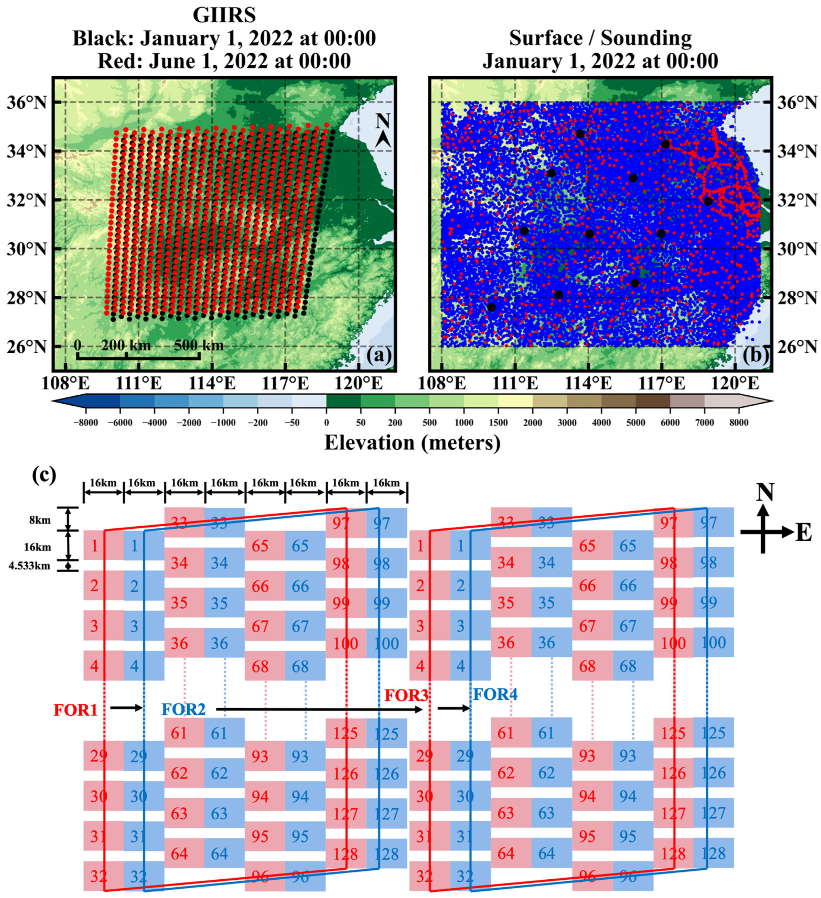
Figure 1. (a) Distribution of GIIRS data (the distribution at 00:00 on 1 January 2022 is indicated by the black dots, and the distribution at 00:00 on 1 June 2022 is indicated by the red dots); (b) Distributions of Ts (red dots), T2m (blue dots) and in situ sounding data (black dots); (c) Scanning mode of GIIRS every two adjacent FORs (after the spring equinox and before the autumn equinox).
Remotesensing 16 01976 g001
Figure 2. (a) MLP model structure; (b) the general framework of the TPE-MLP model.
Remotesensing 16 01976 g002
Figure 3. Mean biases (a) and standard deviations (b) between the retrieved temperature profiles of test set and ERA5 (black, blue, red, green, and orange lines represent the Exp1, Exp2, Exp3, Exp4, and Exp5, respectively).
Remotesensing 16 01976 g003
Figure 4. (a) Variation of the average RMSEs of all pressure levels of the test set with the number of iterations; (b) variation of the minimum value of the average RMSEs with the number of iterations (blue and red represent random search and TPE, respectively; the black dashed line indicates the position of the 20th iteration, the blue dashed line indicates the position where the RMSE of random search reaches its minimum, and the red dashed line indicates the position where the RMSE of TPE reaches its minimum).
Remotesensing 16 01976 g004
Figure 5. Mean biases (a) and standard deviations (b) between the retrieved temperature profiles and ERA5 (black, blue, and red lines represent the training set, validation set, and test set, respectively).
Remotesensing 16 01976 g005
Figure 6. The comparison between retrieval results (a,c) and ERA5 (b,d) at 20:00 on 2 January 2022 ((a,b) represent 500 hPa, (c,d) represent 850 hPa).
Remotesensing 16 01976 g006
Figure 7. (a) Variation of the average RMSEs of all pressure levels of the test set with detectors (black and blue lines represent the time period spans from 1 January to 22 March and 19 September to 31 December and the time period spans from 22 March to 19 September, respectively; red line represents the starting detector positions for the last three columns of detectors). (b) Average NeDT (at 300 K) of each channel for 128 detectors from 22 March to 19 September.
Remotesensing 16 01976 g007
Figure 8. (a) Distribution of the average RMSEs of all pressure levels with the position of the scan sites for the second time period spans; (b) variation of the average RMSEs of all pressure levels with the satellite zenith angles for the second time period spans (red line represents the linear fitted line).
Remotesensing 16 01976 g008
Figure 9. Variation of mean biases with detectors for different pressure levels (ad) represent four detector columns).
Remotesensing 16 01976 g009
Figure 10. Variation of standard deviations with detectors for different pressure levels (ad) represent four detector columns).
Remotesensing 16 01976 g010
Figure 11. (a) Monthly variations of the average RMSEs of all pressure levels of test set (black) and monthly variation of the average standard deviations of all pressure levels of ERA5 temperature (blue line); (b) monthly variations of NeDT (at 300 K).
Remotesensing 16 01976 g011
Figure 12. Monthly variation of mean biases (a) and standard deviations (b) for different pressure levels.
Remotesensing 16 01976 g012
Figure 13. (a) Diurnal variation of the average RMSEs of all pressure levels of the test set (black line) and diurnal variation of the sine of solar altitude angles (blue line); (b) diurnal variation of NeDT (at 300 K).
Remotesensing 16 01976 g013
Figure 14. Diurnal variation of mean biases (a) and standard deviations (b) for different pressure levels.
Remotesensing 16 01976 g014
Figure 15. (a) Mean biases between era5 data and sounding data (black line) and mean biases between retrieved temperature profiles and sounding data (blue line); (b) standard deviations between era5 data and sounding data (black line) and mean biases between retrieved temperature profiles and sounding data (blue line), as well as profile numbers (red line); (c,d) examples of comparisons between sounding profiles (black line), ERA5 profiles (blue line), and retrieved profiles (red line).
Remotesensing 16 01976 g015
Table 1. Formulas of the Activation Function.
NameFormula
relu f x = max   ( x , 0 )
tanh f x = e x e x e x + e x
sigmoid f x = 1 1 + e x
linear f x = x
Table 2. List of Hyperparameters to be Optimized.
Hyper-ParametersRange of Values
Number of hidden layers1, 2, 3, 4, 5
Number of neurons in hidden layer64 to 1024 at intervals of 64
Learning rate1 × 10−2, 1 × 10⁻³, 1 × 10⁻⁴
Patience value2 to 20 at intervals of 2
Activation functionrelu, tanh, sigmoid
Batch size256 to 2560 at intervals of 256
Table 3. List of Sensitivity Experiments for the Input Layer.
Experiment NamesInput of MLP
Exp1GIIRS
Exp2GIIRS + Solar Altitude Angle
Exp3GIIRS + Satellite Zenith Angle
Exp4GIIRS + Ts
Exp5GIIRS + T2m
Table 4. List of Optimized Hyper-parameters.
Hyper-ParametersValue
Number of hidden layers1
Number of neurons in hidden layer832
Learning rate1 × 10−4
Patience value18
Activation functionrelu
Batch size256
Disclaimer/Publisher’s Note: The statements, opinions and data contained in all publications are solely those of the individual author(s) and contributor(s) and not of MDPI and/or the editor(s). MDPI and/or the editor(s) disclaim responsibility for any injury to people or property resulting from any ideas, methods, instructions or products referred to in the content.