Abstract
As the urgency of PM2.5 prediction becomes increasingly ingrained in public awareness, deep-learning methods have been widely used in forecasting concentration trends of PM2.5 and other atmospheric pollutants. Traditional time-series forecasting models, like long short-term memory (LSTM) and temporal convolutional network (TCN), were found to be efficient in atmospheric pollutant estimation, but either the model accuracy was not high enough or the models encountered certain challenges due to their own structure or some specific application scenarios. This study proposed a high-accuracy, hourly PM2.5 forecasting model, poly-dimensional local-LSTM Transformer, namely PD-LL-Transformer, by deep-learning methods, based on air pollutant data and meteorological data, and aerosol optical depth (AOD) data retrieved from the Himawari-8 satellite. This research was based on the Yangtze River Delta Urban Agglomeration (YRDUA), China for 2020–2022. The PD-LL-Transformer had three parts: a poly-dimensional embedding layer, which integrated the advantages of allocating and embedding multi-variate features in a more refined manner and combined the superiority of different temporal processing methods; a local-LSTM block, which combined the advantages of LSTM and TCN; and a Transformer encoder block. Over the test set (the whole year of 2022), the model’s R2 was 0.8929, mean absolute error (MAE) was 4.4523 µg/m3, and root mean squared error (RMSE) was 7.2683 µg/m3, showing great accuracy for PM2.5 prediction. The model surpassed other existing models upon the same tasks and similar datasets, with the help of which a PM2.5 forecasting tool with better performance and applicability could be established.
1. Introduction
PM2.5 comes in many sizes and shapes and can be made up of hundreds of different chemicals. It may interact synergistically to cause adverse respiratory health effects [1] by penetrating deeply into the lungs, irritating and corroding the alveolar wall and, consequently, impairing lung function [2]. In addition, PM2.5 contributes to the heterogeneous reaction of aerosols in the troposphere [3] and the compound pollution effect with O3 and NO2 [4]. Since PM2.5 contributes to a high percentage of all-cause mortalities, among which, for example, as much as 30.2% of ischemic heart disease (IHD), stroke, chronic obstructive pulmonary disease (COPD), and lung cancer (LC) combined had a connection with PM2.5 in 2015 across China [5], it is of great essence for the measurement and estimation of the concentrations of PM2.5.
To better understand and control PM2.5 pollution, coupled with the PM2.5 standards and control policies issued by the governments, more cost-effective monitors and control technologies (devices and materials) are needed [6], but the deployment of the PM2.5 monitoring network on a global scale started late, and the monitoring data reserves of PM2.5 are relatively limited, especially in China [7]. Under this circumstance, satellite observation can be an efficient tool for insight into global long-term changes in ambient PM2.5 concentrations [8]. The satellite-derived AOD and PM2.5 agree in terms of the interannual variability [9], so establishing models using AOD as independent variables to estimate PM2.5 concentration is a promising orientation. Among remote-sensing satellites, MODIS is a commonly used satellite, and many research studies have retrieved PM2.5 from MODIS AOD [10,11]. However, the temporal resolution of MODIS is relatively low, so it is more appropriate to use geostationary satellites with a higher temporal resolution. Himawari-8 is an extraordinary geostationary satellite operated by the Japan Meteorological Agency (JMA, https://www.jma.go.jp/jma/index.html, accessed on 1 January 2023). Launched in 2014, it has the incomparable advantages of 10 min time resolution and 500 m spatial resolution simultaneously, which ensure abundant reliable data are detected and used in distinguished meteorological models. Hourly AOD data could be derived from Himawari-8 and subsequently ensure multiple relevant research studies in China [12,13,14,15].
During the past decade, the machine-learning methods in the field of environmental monitoring and simulation have been expandingly developed and innovated. Many machine-learning models have been applied to atmospheric pollution monitoring or forecasting, such as linear regression (LR) [16], random forest (RF) [17,18], support vector machines or regression (SVM or SVR) [19,20], and XGBoost [21]. Recently, many PM2.5 prediction research studies using the machine-learning approach have been proposed. Mathew et al. [22] utilized machine-learning methods, including LR and gradient boosting, to model daily PM2.5 concentrations in Hyderabad City in India. Vignesh et al. [23] applied linear methods, SVR methods, and tree-based methods to predict daily PM2.5 concentrations across the USA. Karimian et al. [24] successfully used AOD and applied tree-based methods, including random forest (RF), gradient boost, and XGBoost, to predict PM2.5 concentrations over the YRDUA. However, the models are more basic than deep neural networks, and their fitting ability has room for improvement. In recent years, with the development of computing power, deep-learning technologies have gradually entered the public’s view.
As one of the most advanced machine-learning methods, deep-learning models with the basis of neural network architecture have the advantages of being able to perform end-to-end training and abstract representation of advanced features and have achieved remarkable results in the field of environmental modelling [25,26,27,28,29]. The ordinary deep-learning model is multi-layer perceptron (MLP), which could also be called deep neural network (DNN) when the size of the MLP is relatively large. MLPs are excellent base models for the estimation or prediction of atmospheric pollutants. Many MLP-based models were developed, but the simple MLP structures were insufficient to capture adequate information from features. The two main types of MLP updates are the combination of other statistical or machine-learning models [29,30,31] and other attempts to adjust the DNNs. A normal way to update the DNN structure is to import sequential structures into the network so that temporal or sequential information could be learned by the network. Among all the temporal deep-learning models, recurrent neural network (RNN) is the most classical. RNNs add a memory boost to neural networks, making them way smarter when dealing with sequences and patterns. In addition, to avoid the vanishing gradient predicament inherent in ordinary RNNs, long short-term memory (LSTM) [32,33] and gated recurrent unit (GRU) [34] were invented consecutively and became the most popular RNN architectures. RNNs are intrinsically effective for time-series forecasting tasks, including natural language processing (NLP), recommendation system, and stock prediction. In the field of atmospheric particulate matter prediction, RNN-like structures have also been widely used. RNNs are specifically designed for handling sequential data, making them highly suitable for predicting atmospheric particulate matter concentrations, which involve temporal relationships, and RNNs could effectively integrate various data sources, which helps to comprehensively consider the impact of diverse factors on air quality, improving the overall performance of the model [35,36,37,38]. However, RNN-based models have some common ailments, including lack of computational efficiency and suitability for applications involving sequences that are too long. Convolutional neural network (CNN), normally used in spatial processes, could also be used temporally with the one-dimensional structure, where it generally becomes a temporal convolutional network (TCN). TCN is suitable for situations where local information from adjacent temporal points needs to be emphasized [39] but significantly undermines the capability of learning global contents in the time series. In recent years, structures based on an attention mechanism became quite popular, and advanced models were invented based on attention, among which are the revolutionary Transformer [40], bidirectional encoder representations from Transformers (BERT) [41], and generative pre-trained Transformer (GPT) [42]. The involvement of an attention mechanism and other novel adjustments addressed the core challenges faced by RNNs. Beyond the prosperity of NLP, attention-based models or, more specifically, Transformer-based architectures, have also been widely used in atmospheric pollutant forecasting, owing to their excellent adaption with parallelization and avoidance of the vanishing gradient problem while still processing long-range dependencies [43,44,45,46]. However, Transformer still has disadvantages apart from ordinary RNNs, including sequence length limitations and large memory requirements.
As one of the most advanced deep-learning methods, Transformer infrastructures promoted the research in PM2.5 forecasting, but the Transformer-based PM2.5 forecasting models from prior studies were not without room for improvement. Yu et al. [47] built a spatial–temporal Transformer model to realize high-precision PM2.5 prediction in the greater Los Angeles area, but the ST-Transformer model relied on wildfire occurrence as the model input, more or less, which means that the model might not be applicable in different regions or environments, especially the city agglomeration. Wang et al.’s [48] MSAFormer used air pollution data and meteorological data to achieve hourly prediction of PM2.5 in Beijing, the capital of China. Although MSAFormer outperformed other models, including SVM, RF, AdaBoost, LSTM, and GRU, and obtained an R2 of 0.898, an MAE of 8.691 µg/m3, and an RMSE of 11.112 µg/m3, it still had room for optimization. Limperis et al. [49] constructed a TPPM25 model based on Transformer infrastructures to forecast hourly PM2.5 concentrations in Shanghai, the largest city in China, and the model’s MAE was 3.92 µg/m3, but their research only focused on two stations and the research timeframe was only one month, which brought difficulty in spatial and temporal scalability. Therefore, this study intends to explore a high temporal resolution, PM2.5 forecasting, deep-learning model upon the city agglomeration with the integration of different time-series forecasting methods to reduce the disadvantages of the baseline models, and the model should achieve higher predicting accuracy than existing models. In addition, the model should be tested on a larger dataset to enhance the robustness. In this study, we will propose an innovative Transformer-based PM2.5 forecasting model called PD-LL-Transformer. The proposed model not only successfully extracted the sequential information of the atmospheric pollutant and meteorological variable time series but also solved the temporal-reliability and gradient vanishment problems, which normal sequential models encountered. We also performed comparative experiments to illustrate that PD-LL-Transformer surpassed other basic models and was the most suitable model to forecast the PM2.5 concentrations over the YRDUA.
2. Study Area and Materials
2.1. Study Area
Located in east China, the YRDUA (115°46′–123°25′E, 28°05′N–34°50′N; Figure 1) was chosen as the study area. The region was determined by China’s State Council in 2016, consisting of 26 cities in Shanghai, Jiangsu, Zhejiang, and Anhui. With a rich population and strong economy, the YRDUA is deemed as one of the most developed and modernized districts in China. Over the study region, particulate matter concentrations are significant during winter time due to meteorological conditions [50], and air quality over the YRDUA has been substantially improved since 2013 with the introduction of relative laws, policies, or regulations [51]. The atmospheric environmental characteristics of the 26 cities have the feasibility and significance of joint discussion.
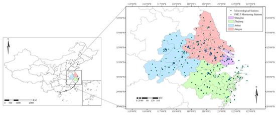
Figure 1.
Geographical location and administrative division of the study area.
2.2. Data Collection
2.2.1. Air Quality Data
Full-year hourly air quality monitoring data from 2020 to 2022 were collected, including the concentrations of PM2.5, PM10, O3, CO, SO2, and NO2 (µg/m3 except CO by mg/m3). In addition, AQI value was also collected. The data were driven from the National Urban Air Quality Real-time Release Platform in China, authorized by the China National Environmental Monitoring Centre (CNEMC, http://www.cnemc.cn/, accessed on 1 January 2023).
Benefiting from the pollution prevention and control policies, the annual average PM2.5 concentration over the YRDUA has had a decreasing trend in general terms in recent years. To calibrate temporal changes in PM2.5, Table 1 shows the annual mean PM2.5 concentrations for the four provinces in the YRDUA (Shanghai, Zhejiang, Jiangsu, and Anhui) from 2020 to 2022, and it also shows the mean concentrations all over the YRDUA. It could be drawn from Table 1 that, in all four provinces except Zhejiang, the annual average concentration of PM2.5 was decreasing year by year. However, there was a slight rebound in 2022 compared to 2021 for PM2.5 concentration in Zhejiang. In addition, Table S1 shows the detailed information of mean PM2.5 concentrations by city in the YRDUA, and in most cities, the mean PM2.5 concentration had a similar decreasing trend in general, while some cities in Zhejiang Province encountered a rising trend from 2021 to 2022. The results showed that, although PM2.5 concentration seemed to decrease from a cursory perspective, the trend was not stable. Therefore, PM2.5 monitoring, prediction, and prevention are still urgent.

Table 1.
The annual mean PM2.5 concentrations (µg/m3) for the four provinces in the YRDUA and for all YRDUA from 2020 to 2022.
2.2.2. Satellite AOD
Himawari-8 is one of the third-generation geostationary weather satellites. Its observation ranges from 80°E to 160°W and from 60°N to 60°S, which can completely cover the research area of the YRDUA. Loaded with AHI, Himawari-8 has a series of mature RS data products, including AOD data that have been calculated and corrected, which can be downloaded from the P-Tree data download platform officially released by JMA (https://www.eorc.jaxa.jp/ptree/ accessed on 1 January 2023).
In this study, the three-year hourly AOD data spanning from 2020 to 2022 were collected. The data had the resolution of 1 h temporally and 5 km × 5 km spatially. The original version of the data was NetCDF, each containing AOD data over 2401 × 2401 grids over regions covering the YRDUA through Himawari-AHI. To match the AOD data with the air quality data indexed by time and location of the monitoring station (the exact longitude and latitude), the original data (2D array indexed by integers) were transferred to a same-shape array indexed by longitude and latitude. To eliminate the bias of matching, a 3-grid interval (15 km × 15 km) was set, and we used the mean AOD value within the interval as the inputting data to reduce the bias of matching. Since light condition significantly influences satellites’ observation on aerosols, AOD could hardly be obtained at night, and even at day, many reasons could lead to missing AOD values, among which are cloud cover or terrain effects. Therefore, the missing ratio of AOD values stayed high. It could be drawn from Figure 2 that the AOD values are generally more abundant during the day, but the missing rate of AOD values overall is approximately 76.08%. From the boxplot in Figure 2, we can observe that the AOD levels looked flat because the ground true distribution of AOD was similar between different hours of the day. The distribution of AOD values is consistent with the distribution of ground level-based PM2.5 concentrations and even that of other concentrations because, on the overall scale, most values fall in a moderate value range, and high values exhibit lower frequency, leading to a positive skewness. Although there was an absence of AOD data to some extent, it is still not appropriate to give up using AOD because it is a relatively crucial feature for PM2.5 forecasting. Therefore, a further innovative and exquisite process is made in this study to solve the problem, and the process is shown in Section 3.2.1.
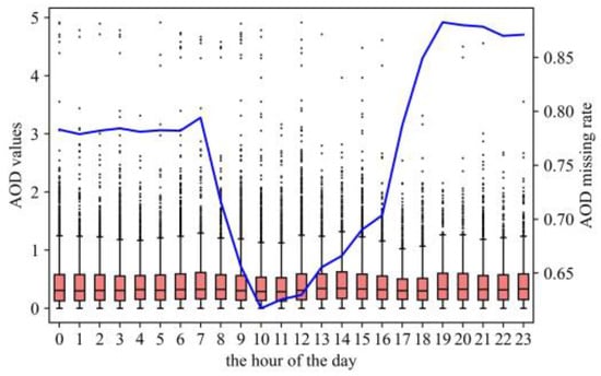
Figure 2.
The boxplot and the missing rate of AOD values (the blue line) for different hours of a day. The left y-axis is the axis of the boxplot, while the right y-axis is the axis of the AOD missing rate line.
2.2.3. Meteorological Data
Wind direction (WD, °), wind speed (WS, m/s), air temperature (TMP, °C), dew point temperature (DPT, °C), and sea-level pressure (PRS_sea, hPa) were 5 meteorological variables used in this research. The hourly data from 2020 to 2022 were downloaded from the National Climatic Data Center (NCDC) affiliated to the National Oceanic and Atmospheric Administration (NOAA) of the United States (https://www.ncei.noaa.gov, accessed on 1 January 2023). The data were hourly or triple-hourly. We filtered the data across China and achieved the data over the YRDUA. There were 187 stations, which are shown in Figure 1. All 5 meteorological feature values are the mean values in an hour. The meteorological data were marked by longitude and latitude and matched with air quality data through Kriging interpolation. Following up was the temporal forward fill of the missing values (using the nearest value forward in time to fill the missing value).
2.2.4. Data Instruction and Preprocessing
The data in Section 2.2.1 and Section 2.2.3 came from 133 main air pollution monitoring sites and 187 meteorological monitoring sites among the YRDUA, which could basically cover the entire research area, shown in Figure 1. To avoid errors caused by using future data in predictions and ensure the practicality of model application in industrial scenarios, the samples were divided strictly by time: data from 1 January 2020 to 31 December 2021 as the training set and that from 1 January 2022 to 31 December 2022 as the test set.
For all the features mentioned, outliers were removed with the use of the interquartile range (IQR) method. We first calculated the 25% quantile value and 75% quantile value of the whole dataset, namely Q1 and Q3, and then we assumed that those values greater than Q3 + 1.5(Q3 − Q1) or smaller than Q1 − 1.5(Q3 − Q1) were outliers. The outliers would be replaced by the boundary values. Additionally, a time series normalization was applied for each station to the train set to eliminate the impact of units and achieve a more uniform distribution of the data as well.
2.3. Deep-Learning Environment
This study was conducted under Windows 10 by Python 3.7. The GPU version of Pytorch was used as the framework for building and running the neural networks. The compute unified device architecture (CUDA) version was NVIDIA CUDA RTX 4090, sourced from OpenBayes, Beijing, China (https://openbayes.com/).
3. Methodologies
3.1. Basics of Deep Learning and Transformer Infrastructure
Originated from perceptron, MLP is a basic type of deep-learning method, with all layers as fully connected layers. In MLPs, information is transmitted between adjacent layers, and all parameters in the network are adjusted by layer-by-layer training. Each layer learns the output features of the previous layer and then obtains a feature vector that is more representative than the input of the upper layer. Most deep-learning models consist of two processes: feed-forward (FF) and back-propagation (BP). The goal of deep-learning models is to optimize the model parameters for minimizing the self-defined loss functions, therefore meeting the objective of the task. The parameters are often adjusted through gradient descent (GD). Most improved GD methods have been developed these years, including stochastic gradient descent (SGD) [52], batch gradient descent (BGD) [53], etc. Adam optimizer is a computationally efficient stochastic optimization algorithm based on adaptive gradient algorithm (AdaGrad) and root mean square propagation (RMSProp) [54] and has been widely used in deep-learning models.
RNN can be considered the most classic means of time-series forecasting. It is widely used in NLP, speech recognition, stock prediction, and image generation. Compared to MLP, RNN introduces the ability to process sequential information. RNNs have internal stats, allowing for the network to retain and utilize previous information when processing sequential data. With the basis of the RNN concept, advanced RNN models have been established and widely used in time-series forecasting tasks, among which are LSTM and GRU. The RNN family has achieved significant success in handling sequential data, but it comes with notable drawbacks. One of them is the vanishing and exploding gradient problem, making it challenging for the network to capture long-term dependencies in processing lengthy sequences. Due to the RNN structure, information passes through weight matrices multiple times, causing the gradient to diminish or explode, limiting the network’s learning capacity.
Apart from RNN, attention is a strong deep-learning mechanism, which allows for models to focus on crucial information when processing sequential data. The core idea of attention is to allocate different weights to different parts of the input sequence, enabling the model to selectively attend to important elements. With the concept of the attention mechanism, Transformer was invented and has been widely used in sequence processing tasks. A typical Transformer model is composed of an encoder and decoder, and the decoder is not necessary dealing with non-NLP tasks. The encoder consists of an embedding layer and several encoder layers. An encoding layer has a multi-head attention part and a linear feed-forward part, each with a corresponding layer and a residual connection net.
The Transformer architecture has gained remarkable prominence across diverse domains. Its innovative self-attention mechanism enables efficient parallelization, and Transformer-based models, such as BERT, GPT, and T5, have demonstrated exceptional performance in tasks.
3.2. Poly-Dimensional Local-LSTM Transformer
In the field of time-series prediction for atmospheric particulate matters, some deep-learning models have been developed, including models based on the RNN architecture or the Transformer architecture. After reviewing and concluding former research, this paper proposed a brand new PM2.5 forecasting model called poly-dimensional local-LSTM Transformer (PD-LL-Transformer).
3.2.1. Combination of Multivariate Features
When encountering missing AOD dilemma in modelling, one efficient way is to divide the dataset into two categories, a dataset with available AOD data and a dataset without AOD data, and then fit the models individually. The division could make the training process more refined. Simultaneously, some other features could be applied to the same process. For instance, since PM2.5 has seasonal trends, researchers could divide the dataset by season and model them separately. Different stations have different populational, economical, and traffic impacts on PM2.5 emissions; therefore, dividing the dataset by station and modeling them individually could bring improvements. The differences between each individual sub-dataset could be regarded as patterns. Based on this concept, we developed a poly-dimensional embedding (PD) infrastructure, which combined multivariate features together to make the deep-learning model learn different patterns through the training process.
In PM2.5 forecasting tasks, common features, including meteorological variables and air quality variables, are continuous numerical data. However, the formation of PM2.5 highly relies on some non-numerical classification features or numerical regression features. Compared to those normal numerical-input models, PD-LL-Transformer included eight concrete classification features: station, season, hour-of-the-day, month-of-the-year, AOD availability, current PM2.5 level, current O3 level, and current AQI level. Among these features, station enables the model to extract spatial information of the model, and season, month-of-the-year, and hour-of-the-day represent temporality. PM2.5 level, O3 level, and AQI level are regulated by the Ambient Air Quality Standards [55] and Technical Regulation on Ambient Air Quality Index (on trail) [56] issued by the Ministry of Environmental Protection of the People’s Republic of China. As is mentioned in Section 2.2.2, satellite AOD is strongly correlated with PM2.5 concentrations, but the availability of AOD data is challenging. Therefore, PD-LL-Transformer takes AOD availability as an extra binary classification feature on top of simply using continuous AOD values. For data points whose AOD value is missing, its AOD value is replaced by zero, and its AOD availability is set different from other data points with correct AOD value. Since real AOD values range from 0 to 1, there is no need to standardize the AOD values. This novel process empowers the model to learn both the AOD information to influence PM2.5 concentrations and the scenarios when the AOD value is missing.
Most models use one-hot encoding to encode concrete features. One-hot encoding leads to high-dimensional sparse vectors and may cause the loss of some crucial information. PD-LL-Transformer uses parallel embedding layers rather than one-hot encoding to deal with concrete features. The embedding dims for different features are set respectively, specifically according to their unique characteristics and original number of categories. The detailed information for the concrete features and embedding dims is presented in Table 2. The embedding process of different features is independent, and the embedding results are concatenated with numerical continuous raw features to form the new input features for subsequent parts of the model.
Table 2.
The detailed information for the concrete features in the PD embedding layers.
3.2.2. Local-LSTM Transformer
Although the Transformer succeeded in many sequence tasks, the standard Transformer architecture failed to deal with local information in the sequence. Neither is basic RNN architecture able to extract local information; therefore, many convolutional layer-RNNs were developed to fill this gap. Inspired by the idea of R-Transformer, which managed to combine the RNN and Transformer together, PD-LL-Transformer has the structure of a 1 D convolutional LSTM (local LSTM) to capture the local information of a sequence and, hence, enhance the control of long-term dependencies.
An ordinary LSTM has a cell state series, which ought to be modified through time, emphasizing the sequential nature of the time series at the expense of localization, and PD-LL-Transformer’s LSTM cells are localized, which means that they are modified not only along adjacent or nearby positions but are also feasible for parallelization while computing. Local LSTM combined the advantages of both LSTM and CNN structures, allowing for the layer to focus on long sequences of information and to add local information as a supplement. After the local-LSTM layer, the sequence would enter a normal multi-head attention layer like a normal Transformer. PD-LL-Transformer is an integrated deep-learning model that draws on the strengths of embedding, CNN, RNN, and Transformer to make up for the corresponding weaknesses. The general structure and hyper parameters of PD-LL-Transformer are shown in Figure 3 and Table 3, respectively. The label was the PM2.5 concentrations for the next hour at each timestep, and the input was the features in the past 24 h as the default, which means that the model mapped 24 timestep features to 1 timestep label. The number of timesteps would be modified and discussed further in Section 4.3.
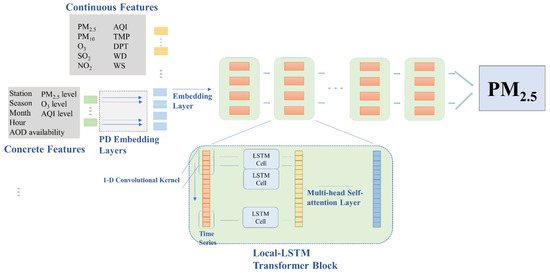
Figure 3.
The basic structure of PD-LL-Transformer.
Table 3.
The hyper parameters of PD-LL-LSTM and illustrations of the whole task.
4. Results and Analysis
4.1. Model Performance
In this study, we compared several different models (MLP, LSTM, PD-Transformer, and PD-LL-Transformer) by their performance on the exact same training set and test set. The former two classic models were set as the benchmarks to show the enhancement brought by the poly-dimensional combination of multivariate features, and PD-Transformer was a superior benchmark with the application of poly-dimensional combination architecture, to examine the efficiency of the convolutional LSTM process in PD-LL-Transformer. The models were trained with the loss of L2 loss (MSE loss), and R2, MAE (µg/m3), and RMSE (µg/m3) for the test set (out sample) were set as the evaluation metrics. The evaluation results are shown in Table 4 and Table 5.
Table 4.
Performances of the four models over the test set.
Table 5.
Enhancement metrics of PD-LL-Transformer over the test set.
As is shown in Table 5, PD-LL-Transformer has the best performance among the four models. Compared to the suboptimal PD-Transformer, PD-LL-Transformer amplified R2 by 2.03% and cut MAE by 21.39% and RMSE by 9.48%, respectively. The results showed that PD-LL-Transformer has exhibited a significant improvement in terms of precision with the help of capturing patterns and relationship within the input features from multiple dimensions. Furthermore, to better illustrate the effectiveness of PD-LL-Transformer, we analyzed the results of each station individually. In Figure 4, R2, MAE, and RMSE over different individual stations from different models were analyzed. In addition, Figure 5 shows the results from four groups divided by province (the information of stations was in Table S2). Both Figure 4 and Figure 5 show that PD-LL-Transformer is capable of beating the other models in most situations. In addition, considering the result by province, PD-LL-Transformer also outperformed the other models.
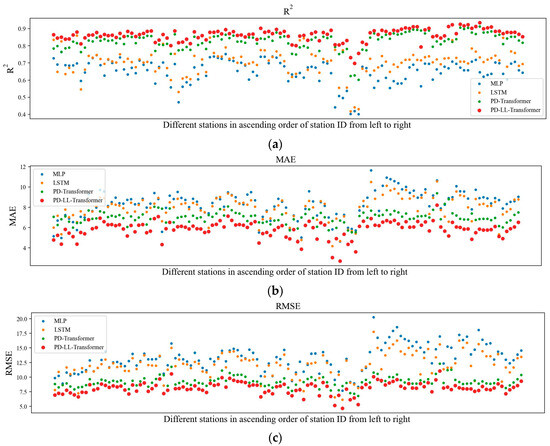
Figure 4.
(a) R2, (b) MAE, and (c) RMSE for the four models at all individual stations in the test set. The points that indicate performances of PD-LL-Transformer are bold in red.
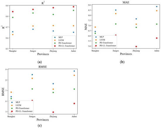
Figure 5.
(a) R2, (b) MAE, and (c) RMSE for the four models at four provinces in the test set. The points that indicate performances of PD-LL-Transformer are bold in red.
4.2. Pollution Trends
With the application of PD-LL-Transformer, we generated the mean value of PM2.5 concentrations forecast results for all YRDUA stations for the entire time range of the test set (in the year 2022). Additionally, we compared those predictions to the real PM2.5 concentrations to examine model performance. The trend of PM2.5 pollution of the whole YRDUA is shown in Figure 6. The two curves, standing for predicted values and real values, closely match and overlap each other, confirming the efficacy of PD-LL-Transformer. We found that the difference between the metrics of the training set and those of the test set is relatively small, which means that over-fitting was avoided successfully. The results might be drawn from the temporal homogeneity of atmospheric features and meteorological features. Therefore, PD-LL-Transformer has the potential of better performances in the future with an expansion of the multi-variate data size.
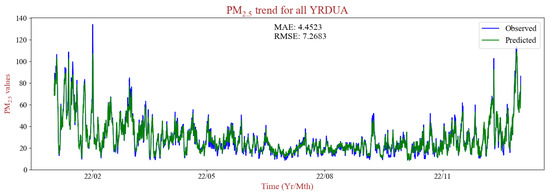
Figure 6.
The predicted and the real trends of PM2.5 pollution in 2022 over the YRDUA.
To more specifically illustrate the high-precision prediction throughout the temporal range, Figure 7 shows the trends of average PM2.5 concentrations and the predicted concentrations over the YRDUA over the test set. As Figure 7 shows, PD-LL-Transformer is competent not only in predicting the overall PM2.5 pollution situation but also in forecasting PM2.5 trends in specific months. The predicted values were broadly close to the measured values. As for the interpretation of PD-LL-Transformer’s spatial practicality, we conclude that the acquisition of the spatial information comes from two aspects: one is the variation in the inherent characteristics of ordinary features across different locations, and the other is the embedding process of the station feature in the poly-dimensional application.
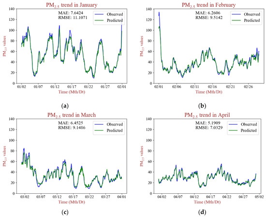
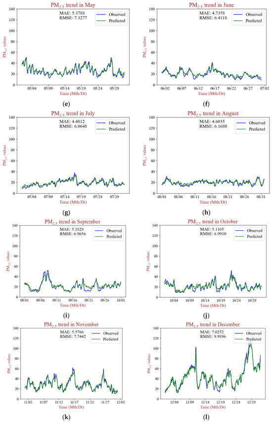
Figure 7.
The predicted and the real trends of PM2.5 pollution in different months of 2022 over the YRDUA. (a–l) stand for 12 months through 2022.
In addition, Figure 8 shows the boxplots of the observed PM2.5 concentration values and the predicted PM2.5 concentration values for each month in 2022. It could be drawn from the plots that, in each month, the observed values and the predicted values roughly follow similar distributions, demonstrating high levels of fit.
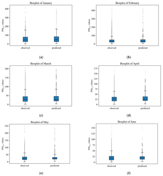
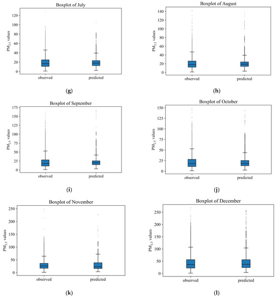
Figure 8.
The boxplots of predicted and the realPM2.5 concentrations in different months of 2022 over the YRDUA. (a–l) stand for 12 months through 2022.
4.3. Different-Hour Predictions
The basic procedure of the research was based on using data from the past 24 h to predict the scenario in the next hour. The size of the window text was set based on experience. To better generalize the model and enhance the persuasiveness of the model’s advantages, we performed experiments on different window sizes (1 h, 2 h, 3 h, 6 h, and 12 h). Except MLP, which always only took the information at the last timestep as the model input, LSTM, PD-Transformer, and PD-LL-Transformer, all as the time-series model, learned different temporal information given sequences with different timesteps.
Figure 9 shows the evaluation metrics for the test set for the four models at different window sizes. We could elucidate from the figures that PD-LL-Transformer has the best performance among the models, and the excellency remains through the modification of timesteps. For the different window texts in a day (1 h, 2 h, 3 h, 6 h, 12 h, and 24 h), PD-LL-Transformer always outperforms the other models horizontally. In addition, an interesting phenomenon is that, at the level of short forecasting window, normal LSTM architecture is even inferior to ordinary MLP, which is reasonable since RNNs mainly rely on the learnability of the time sequence and a shorter period of data might be insufficient for LSTM to learn the information from the data; hence, LSTM showed lower precision than MLP. LSTM, PD-Transformer, and PD-LL-Transformer are time-series models upon which different window sizes have different impacts, and theoretically, the greater the window size is, the better performance the model could achieve, hence reducing MAE and RMSE. Compared with Transformer-based models, LSTM is a more trivial model, so its performance has obvious promotion as the hour increases, while PD-Transformer and PD-LL-Transformer has only slight promotion under the same circumstances because their infrastructures are intrinsically advanced. As a matter of fact, Transformer architecture with a poly-dimensional frame could effectively avoid this dilemma, especially for PD-LL-Transformer, which showed a slight difference in model performance as the timestep changed. Therefore, PD-LL-Transformer also has temporal robustness.
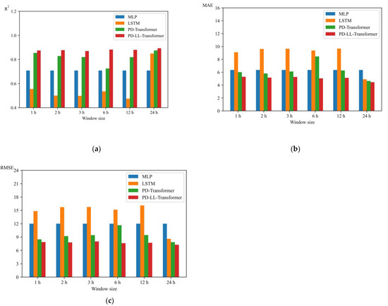
Figure 9.
(a) R2, (b) MAE, and (c) RMSE for the four models at different window sizes.
4.4. Spatio Distribution of Prediction
Figure 10 shows the distribution map of prediction bias and absolute error over the stations from PD-LL-Transformer. It could be drawn from Figure 10a that the MAEs of most stations range from 4 µg/m3 to 6 µg/m3, which are at low levels overall and consistent with the overall predictive effect of the model. According to Figure 10b, the mean residuals of most stations are close to 0, showing that PD-LL-Transformer has good forecasting ability for PM2.5 concentrations over the YRDUA.
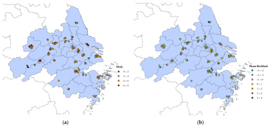
Figure 10.
(a) MAE and (b) mean residual for PD-LL-Transformer at different window sizes.
5. Conclusions and Discussions
This study was motivated by the severity of pollution caused by PM2.5 and finished under the framework of deep learning. The main contribution of this study was a novel PD-LL-Transformer to forecast PM2.5 concentrations. In this study, we solved two main problems: (1) proposed PD-LL-Transformer as the state-of-the-art, machine-learning based hourly PM2.5 prediction technique over the YRDUA, which could contribute to effective environmental monitoring, aiding authorities in assessing air quality and implementing timely interventions to address pollution issues; and (2) further promoted the organic integration of deep-learning models with the prediction of atmospheric particulate matter concentrations, playing a significant role in the field of deep-learning models. There is a structurally inherent compatibility existing between PD-LL-Transformer and multi-variate data, so PD-LL-Transformer also has the potential to be more excellent as the data source is more abundant. Beyond the major contributions, this study also provided some innovative insights: the fully spatial and temporal combination of atmospheric and meteorological information, the practical and adequate AOD application in PM2.5 forecasting, and the expansion of time-series forecasting, deep-learning models. In addition, this study also finished additional experiments at window-size and station-respective scales to convince the usefulness and power of PD-LL-Transformer. At distinguished stations and with the use of data of different hours of time, PD-LL-Transformer almost always beat the traditional models.
Compared with existing deep-learning models that focus on PM2.5 forecasting, PD-LL-Transformer has several advantages. (1) The key idea of PD-LL-Transformer is the appropriate application of diverse features and the organic combination of different deep-learning infrastructures, which has reference value. (2) PD-LL-Transformer has potential applicability in most regions since its input features, though from multi-variate source, are comparatively easy to achieve. Compared with models that include rare features such as wildfire and models that rely on more strict situations, PD-LL-Transformer is suitable for large urban agglomerations such as the YRDUA. (3) Compared with daily PM2.5 forecasting, PD-LL-Transformer is hourly-based, which brings higher temporal resolution. In addition, among the hourly-based PM2.5 forecasting models, PD-LL-Transformer has greater fitting capability. The MAE of 4.4523 µg/m3 and the RMSE of 7.2683 µg/m3 over the test set are lower than most existing PM2.5 hourly forecasting models.
About further research, we propose two aspects for improvements: the greater refinement of data collection and preprocessing and the detailed interpretation process of the deep-learning model. PD-LL-Transformer was constructed based on studies at different stations in the YRDUA overall. Although the poly-dimensional embedding process made it feasible for the model to learn the spatial distribution of atmospheric and meteorological features, a more refined supplement of data could be applied to broaden the locational applicability. PD-LL-Transformer, as a supervised learning model, could be integrated with unsupervised learning architecture with regard to fully topographical prediction. In addition, the interpretational analysis of the attention mechanism, serving as the core concept of PD-LL-Transformer, could be explored further.
Supplementary Materials
The following supporting information can be downloaded at: https://www.mdpi.com/article/10.3390/rs16111915/s1, Table S1. The annual mean PM2.5 concentrations (µg/m3) for the distinguished cities in the YRDUA from 2020 to 2022. Table S2. Information of all stations.
Author Contributions
Conceptualization, R.Z. and L.Z.; project administration, R.Z.; resources, R.Z., X.L. and L.Z.; methodology, R.Z.; software, R.Z. and L.Z.; data curation, H.H. and L.Z.; validation, H.H.; visualization, R.Z. and H.H.; investigation, F.Z.; writing—original draft preparation, R.Z.; writing—review and editing H.H., C.R., W.W. and L.Z.; project administration, L.Z.; supervision, L.Z. and X.D.; funding acquisition, L.Z. All authors have read and agreed to the published version of the manuscript.
Funding
This work was jointly funded by the Humanities and Social Sciences Program of the Ministry of Education of China (23YJAZH223), Key Laboratory of Spatial–temporal Big Data Analysis and Application of Natural Resources in Megacities, MNR (KFKT-2022-06), and National Natural Science Foundation of China (41001234).
Data Availability Statement
Data are contained within the article.
Conflicts of Interest
The authors declare no conflict of interest.
References
- Wu, S.; Deng, F.; Hao, Y.; Wang, X.; Zheng, C.; Lv, H.; Lu, X.; Wei, H.; Huang, J.; Qin, Y.; et al. Fine particulate matter, temperature, and lung function in healthy adults: Findings from the HVNR study. Chemosphere 2014, 108, 168–174. [Google Scholar] [CrossRef] [PubMed]
- Xing, Y.F.; Xu, Y.H.; Shi, M.H.; Lian, Y.X. The impact of PM2.5 on the human respiratory system. J. Thorac. Dis. 2016, 8, E69–E74. [Google Scholar] [CrossRef] [PubMed]
- Ravishankara, A.R. Heterogeneous and multiphase chemistry in the troposphere. Science 1997, 276, 1058–1065. [Google Scholar] [CrossRef]
- Crouse, D.L.; Peters, P.A.; Hystad, P.; Brook, J.R.; van Donkelaar, A.; Martin, R.V.; Villeneuve, P.J.; Jerrett, M.; Goldberg, M.S.; Pope, C.A., 3rd; et al. Ambient PM2.5, O3, and NO2 Exposures and Associations with Mortality over 16 Years of Follow-Up in the Canadian Census Health and Environment Cohort (CanCHEC). Environ. Health Perspect. 2015, 123, 1180–1186. [Google Scholar] [CrossRef] [PubMed]
- Song, C.B.; He, J.J.; Wu, L.; Jin, T.S.; Chen, X.; Li, R.P.; Ren, P.P.; Zhang, L.; Mao, H.J. Health burden attributable to ambient PM2.5 in China. Environ. Pollut. 2017, 223, 575–586. [Google Scholar] [CrossRef] [PubMed]
- Liang, C.S.; Duan, F.K.; He, K.B.; Ma, Y.L. Review on recent progress in observations, source identifications and countermeasures of PM2.5. Environ. Int. 2016, 86, 150–170. [Google Scholar] [CrossRef] [PubMed]
- Chan, C.K.; Yao, X. Air pollution in mega cities in China. Atmos. Environ. 2008, 42, 1–42. [Google Scholar] [CrossRef]
- van Donkelaar, A.; Martin, R.V.; Brauer, M.; Boys, B.L. Use of Satellite Observations for Long-Term Exposure Assessment of Global Concentrations of Fine Particulate Matter. Environ. Health Perspect. 2015, 123, 135–143. [Google Scholar] [CrossRef] [PubMed]
- Li, J.; Carlson, B.E.; Lacis, A.A. How well do satellite AOD observations represent the spatial and temporal variability of PM2.5 concentration for the United States? Atmos. Environ. 2015, 102, 260–273. [Google Scholar] [CrossRef]
- Fu, D.S.; Song, Z.J.; Zhang, X.L.; Xia, X.G.; Wang, J.; Che, H.Z.; Wu, H.J.; Tang, X.; Zhang, J.Q.; Duan, M.Z. Mitigating MODIS AOD non-random sampling error on surface PM2.5 estimates by a combined use of Bayesian Maximum Entropy method and linear mixed-effects model. Atmos. Pollut. Res. 2020, 11, 482–490. [Google Scholar] [CrossRef]
- Yang, Z.M.; Zdanski, C.; Farkas, D.; Bang, J.; Williams, H. Evaluation of Aerosol Optical Depth (AOD) and PM2.5 associations for air quality assessment. Remote Sens. Appl.-Soc. Environ. 2020, 20, 100396. [Google Scholar] [CrossRef]
- Hu, K.Y.; Guo, X.L.; Gong, X.Y.; Wang, X.P.; Liang, J.Q.; Li, D.Q. Air quality prediction using spatio-temporal deep learning. Atmos. Pollut. Res. 2022, 13, 101543. [Google Scholar] [CrossRef]
- Li, Y.; Xue, Y.; Guang, J.; She, L.; Chen, G.L.; Fan, C. Hourly Ground Level PM2.5 Estimation for the Southeast of China Based on Himawari-8 Observation Data. In Proceedings of the IEEE International Geoscience and Remote Sensing Symposium (IGARSS), Yokohama, Japan, 28 July–2 August 2019; pp. 7850–7853. [Google Scholar]
- Song, Z.; Chen, B.; Huang, J. Combining Himawari-8 AOD and deep forest model to obtain city-level distribution of PM2.5 in China. Environ. Pollut. 2022, 297, 118826. [Google Scholar] [CrossRef] [PubMed]
- Xue, Y.; Li, Y.; Guang, J.; Tugui, A.; She, L.; Qin, K.; Fan, C.; Che, Y.H.; Xie, Y.Q.; Wen, Y.N.; et al. Hourly PM2.5 Estimation over Central and Eastern China Based on Himawari-8 Data. Remote Sens. 2020, 12, 855. [Google Scholar] [CrossRef]
- Gad, I.M.; Doreswamy, H.; Harishkumar, K.S.; Km, Y. Forecasting Air Pollution Particulate Matter (PM2.5) Using Machine Learning Regression Models. Procedia Comput. Sci. 2020, 171, 2057–2066. [Google Scholar]
- Chen, G.; Li, S.; Knibbs, L.D.; Hamm, N.A.S.; Cao, W.; Li, T.; Guo, J.; Ren, H.; Abramson, M.J.; Guo, Y. A machine learning method to estimate PM2.5 concentrations across China with remote sensing, meteorological and land use information. Sci. Total Environ. 2018, 636, 52–60. [Google Scholar] [CrossRef] [PubMed]
- Chen, X.L.; Li, H.; Zhang, S.T.; Chen, Y.Z.; Fan, Q. High Spatial Resolution PM2.5 Retrieval Using MODIS and Ground Observation Station Data Based on Ensemble Random Forest. IEEE Access 2019, 7, 44416–44430. [Google Scholar] [CrossRef]
- Li, H.Q.; Shi, X.H. Data Driven based PM2.5 Concentration Forecasting. In Proceedings of the International Conference on Biological Engineering and Pharmacy (BEP), Shanghai, China, 9–11 December 2016; pp. 301–304. [Google Scholar]
- Zhou, Y.; Chang, F.J.; Chang, L.C.; Kao, I.F.; Wang, Y.S.; Kang, C.C. Multi-output support vector machine for regional multi-step-ahead PM2.5 forecasting. Sci. Total Environ. 2019, 651, 230–240. [Google Scholar] [CrossRef]
- Dai, H.B.; Huang, G.Q.; Zeng, H.B.; Zhou, F.Y. PM2.5 volatility prediction by XGBoost-MLP based on GARCH models. J Clean Prod. 2022, 356, 131898. [Google Scholar] [CrossRef]
- Mathew, A.; Gokul, P.R.; Shekar, P.R.; Arunab, K.S.; Abdo, H.G.; Almohamad, H.; Al Dughairi, A.A. Air quality analysis and PM2.5 modelling using machine learning techniques: A study of Hyderabad city in India. Cogent Eng. 2023, 10, 2243743. [Google Scholar] [CrossRef]
- Vignesh, P.P.; Jiang, J.H.; Kishore, P. Predicting PM2.5 Concentrations Across USA Using Machine Learning. Earth Space Sci. 2023, 10, e2023EA002911. [Google Scholar] [CrossRef]
- Karimian, H.; Li, Y.Q.; Chen, Y.L.; Wang, Z.R. Evaluation of different machine learning approaches and aerosol optical depth in PM2.5 prediction. Environ. Res. 2023, 216, 114465. [Google Scholar] [CrossRef] [PubMed]
- Gupta, P.; Christopher, S.A. Particulate matter air quality assessment using integrated surface, satellite, and meteorological products: Multiple regression approach. J. Geophys. Res. Atmos. 2009, 114, D14205. [Google Scholar] [CrossRef]
- Gupta, P.; Christopher, S.A. Particulate matter air quality assessment using integrated surface, satellite, and meteorological products: 2. A neural network approach. J. Geophys. Res. Atmos. 2009, 114. [Google Scholar] [CrossRef]
- Lee, C.; Lee, K.; Kim, S.; Yu, J.; Jeong, S.; Yeom, J. Hourly Ground-Level PM2.5 Estimation Using Geostationary Satellite and Reanalysis Data via Deep Learning. Remote Sens. 2021, 13, 2121. [Google Scholar] [CrossRef]
- Li, T.W.; Shen, H.F.; Yuan, Q.Q.; Zhang, X.C.; Zhang, L.P. Estimating Ground-Level PM2.5 by Fusing Satellite and Station Observations: A Geo-Intelligent Deep Learning Approach. Geophys. Res. Lett. 2017, 44, 11985–11993. [Google Scholar] [CrossRef]
- Sun, Y.B.; Zeng, Q.L.; Geng, B.; Lin, X.W.; Sude, B.; Chen, L.F. Deep Learning Architecture for Estimating Hourly Ground-Level PM2.5 Using Satellite Remote Sensing. IEEE Geosci. Remote Sens. Lett. 2019, 16, 1343–1347. [Google Scholar] [CrossRef]
- Lu, X.M.; Wang, J.J.; Yan, Y.T.; Zhou, L.G.; Ma, W.C. Estimating hourly PM2.5 concentrations using Himawari-8 AOD and a DBSCAN-modified deep learning model over the YRDUA, China. Atmos. Pollut. Res. 2021, 12, 183–192. [Google Scholar] [CrossRef]
- Wang, Z.; Li, R.Y.; Chen, Z.Y.; Yao, Q.; Gao, B.B.; Xu, M.Q.; Yang, L.; Li, M.C.; Zhou, C.H. The estimation of hourly PM2.5 concentrations across China based on a Spatial and Temporal Weighted Continuous Deep Neural Network (STWC-DNN). ISPRS J. Photogramm. Remote Sens. 2022, 190, 38–55. [Google Scholar] [CrossRef]
- Hochreiter, S.; Schmidhuber, J. Bridging long time lags by weight guessing and “long short term memory”. In Proceedings of the Sintra Workshop on Spatiotemporal Models in Biological and Artificial Systems, Sintra, Portugal, 6–8 November 1996; pp. 65–72. [Google Scholar]
- Zhang, Y.Y.; Sun, Q.S.; Liu, J.; Petrosian, O. Long-Term Forecasting of Air Pollution Particulate Matter (PM2.5) and Analysis of Influencing Factors. Sustainability 2024, 16, 19. [Google Scholar] [CrossRef]
- Cho, K.; Van Merrienboer, B.; Gulcehre, C.; Bahdanau, D.; Bougares, F.; Schwenk, H.; Bengio, Y. Learning Phrase Representations using RNN Encoder-Decoder for Statistical Machine Translation. arXiv 2014, arXiv:1406.1078. [Google Scholar]
- Ding, C.; Wang, G.Z.; Zhang, X.Y.; Liu, Q.; Liu, X.D. A hybrid CNN-LSTM model for predicting PM2.5 in Beijing based on spatiotemporal correlation. Environ. Ecol. Stat. 2021, 28, 503–522. [Google Scholar] [CrossRef]
- Kim, H.S.; Han, K.M.; Yu, J.; Kim, J.; Kim, K.; Kim, H. Development of a CNN plus LSTM Hybrid Neural Network for Daily PM2.5 Prediction. Atmosphere 2022, 13, 2124. [Google Scholar] [CrossRef]
- Li, D.; Liu, J.P.; Zhao, Y.Y. Prediction of Multi-Site PM2.5 Concentrations in Beijing Using CNN-Bi LSTM with CBAM. Atmosphere 2022, 13, 1719. [Google Scholar] [CrossRef]
- Li, T.Y.; Hua, M.; Wu, X. A Hybrid CNN-LSTM Model for Forecasting Particulate Matter PM2.5. IEEE Access 2020, 8, 26933–26940. [Google Scholar] [CrossRef]
- Zhu, M.Y.; Xie, J. Investigation of nearby monitoring station for hourly PM2.5 forecasting using parallel multi-input 1D-CNN-biLSTM. Expert Syst. Appl. 2023, 211, 118707. [Google Scholar] [CrossRef]
- Vaswani, A.; Shazeer, N.; Parmar, N.; Uszkoreit, J.; Jones, L.; Gomez, A.N.; Kaiser, Ł.; Polosukhin, I. Attention is all you need. Adv. Neural Inf. Process. Syst. 2017, 30. Available online: https://arxiv.org/abs/1706.03762 (accessed on 14 April 2024).
- Devlin, J.; Chang, M.W.; Lee, K.; Toutanova, K. BERT: Pre-training of Deep Bidirectional Transformers for Language Understanding. arXiv 2018, arXiv:1810.04805. [Google Scholar]
- Radford, A.; Narasimhan, K.; Salimans, T.; Sutskever, I. Improving Language Understanding by Generative Pre-Training. 2018. Available online: https://www.mikecaptain.com/resources/pdf/GPT-1.pdf (accessed on 14 April 2024).
- Tong, W.T.; Limperis, J.; Hamza-Lup, F.; Xu, Y.; Li, L.X. Robust Transformer-based model for spatiotemporal PM2.5 prediction in California. Earth Sci. Inform. 2023. [Google Scholar] [CrossRef]
- Verma, A.; Ranga, V.; Vishwakarma, D.K. A novel approach for forecasting PM2.5 pollution in Delhi using CATALYST. Environ. Monit. Assess. 2023, 195, 1457. [Google Scholar] [CrossRef]
- Zeng, Q.L.; Wang, L.H.; Zhu, S.Y.; Gao, Y.H.; Qiu, X.F.; Chen, L.F. Long-term PM2.5 concentrations forecasting using CEEMDAN and deep Transformer neural network. Atmos. Pollut. Res. 2023, 14, 101839. [Google Scholar] [CrossRef]
- Zhang, Z.; Zhang, S. Modeling air quality PM2.5 forecasting using deep sparse attention-based transformer networks. Int. J. Environ. Sci. Technol. 2023, 20, 13535–13550. [Google Scholar] [CrossRef]
- Yu, M.Z.; Masrur, A.; Blaszczak-Boxe, C. Predicting hourly PM2.5 concentrations in wildfire-prone areas using a SpatioTemporal Transformer model. Sci. Total Environ. 2023, 860, 160446. [Google Scholar] [CrossRef] [PubMed]
- Wang, H.Q.; Zhang, L.F.; Wu, R. MSAFormer: A Transformer-Based Model for PM2.5 Prediction Leveraging Sparse Autoencoding of Multi-Site Meteorological Features in Urban Areas. Atmosphere 2023, 14, 1294. [Google Scholar] [CrossRef]
- Limperis, J.; Tong, W.T.; Hamza-Lup, F.; Li, L.X. PM2.5 forecasting based on transformer neural network and data embedding. Earth Sci. Inform. 2023, 16, 2111–2124. [Google Scholar] [CrossRef]
- Li, L.; Chen, C.H.; Fu, J.S.; Huang, C.; Streets, D.G.; Huang, H.Y.; Zhang, G.F.; Wang, Y.J.; Jang, C.J.; Wang, H.L.; et al. Air quality and emissions in the Yangtze River Delta, China. Atmos. Chem. Phys. 2011, 11, 1621–1639. [Google Scholar] [CrossRef]
- Zhang, C.Y.; Zhao, L.; Zhang, H.T.; Chen, M.N.; Fang, R.Y.; Yao, Y.; Zhang, Q.P.; Wang, Q. Spatial-temporal characteristics of carbon emissions from land use change in Yellow River Delta region, China. Ecol. Indicators 2022, 136, 108623. [Google Scholar] [CrossRef]
- Meuleau, N.; Dorigo, M. Ant colony optimization and stochastic gradient descent. Artif Life 2002, 8, 103–121. [Google Scholar] [CrossRef]
- Saeed, U.; Ahmad, S.; Alsadi, J.; Ross, D.; Rizvi, G. Implementation Of Neural Network For Color Properties Of Polycarbonates. In Proceedings of the 29th International Conference of the Polymer-Processing-Society (PPS), Nuremberg, Germany, 15–19 July 2013; pp. 56–59. [Google Scholar]
- Kingma, D.; Ba, J. Adam: A Method for Stochastic Optimization. arXiv 2014, arXiv:1412.6980. [Google Scholar]
- GB 3095-2012; Ambient Air Quality Standards. Ministry of Ecology and Environment of the People’s Republic of China: Beijing, China, 2012. Available online: https://www.chinesestandard.net/PDF.aspx/GB3095-2012 (accessed on 14 April 2024).
- HJ 633-2012; Technical Regulation on Ambient Air Quality Index (on trial). Ministry of Ecology and Environment of the People’s Republic of China: Beijing, China, 2012. Available online: https://www.chinesestandard.net/PDF.aspx/HJ633-2012 (accessed on 14 April 2024).
Disclaimer/Publisher’s Note: The statements, opinions and data contained in all publications are solely those of the individual author(s) and contributor(s) and not of MDPI and/or the editor(s). MDPI and/or the editor(s) disclaim responsibility for any injury to people or property resulting from any ideas, methods, instructions or products referred to in the content. |
© 2024 by the authors. Licensee MDPI, Basel, Switzerland. This article is an open access article distributed under the terms and conditions of the Creative Commons Attribution (CC BY) license (https://creativecommons.org/licenses/by/4.0/).