


Adaptive Learnable Spectral–Spatial Fusion Transformer for Hyperspectral Image Classification

Abstract
1. Introduction
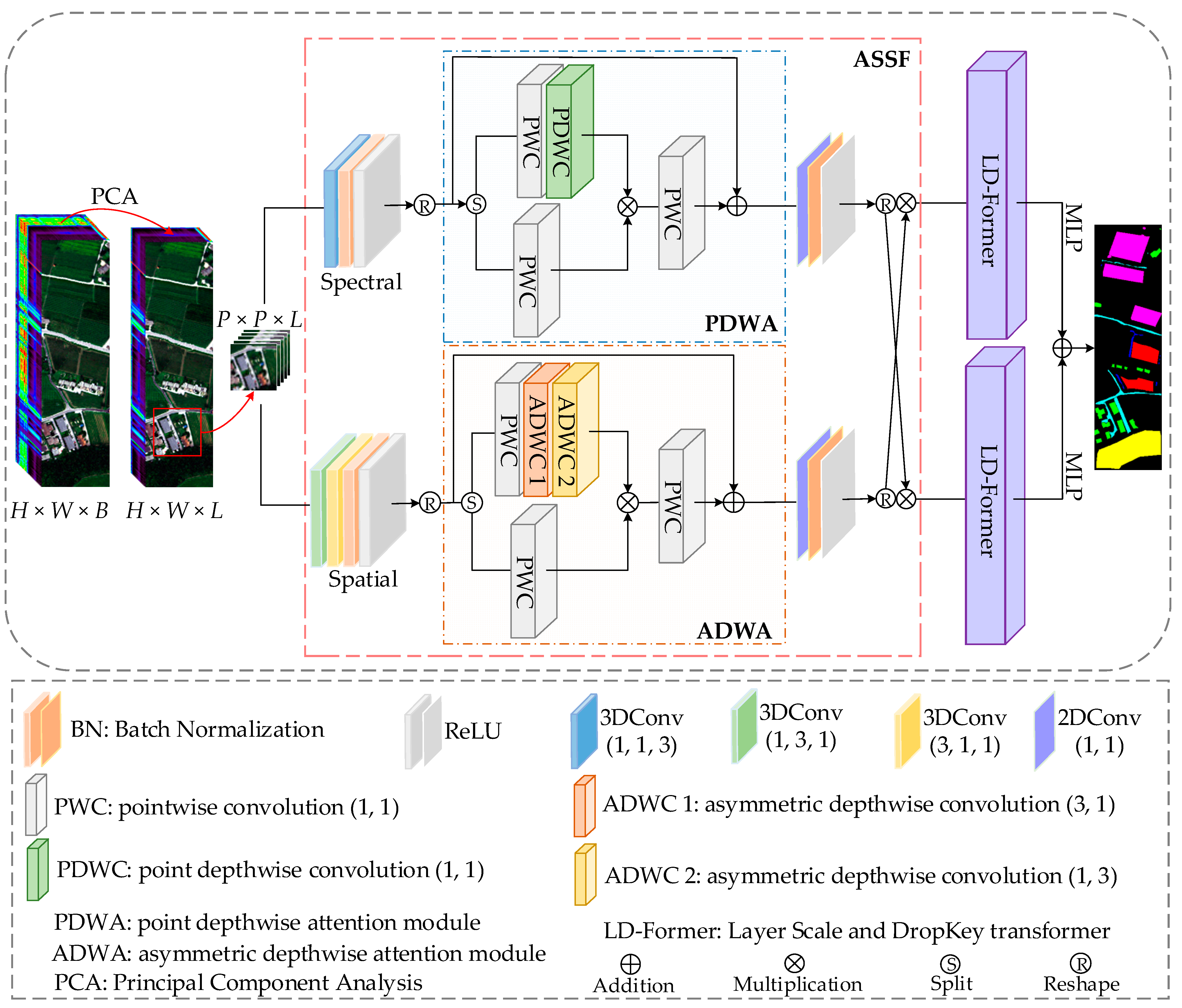
- In this study, a dual-branch fusion model named ALSST is designed to extract the spectral–spatial fusion features of HSIs. This model synergistically combines the prowess of CNNs in extracting local features with the capacity of a vision transformer to discern long-range dependencies. Through this integrated approach, the ALSST aims to provide a comprehensive learning mechanism for the spectral–spatial fusion features of HSIs, optimizing the ability of the model to interpret and classify complex hyperspectral data effectively.
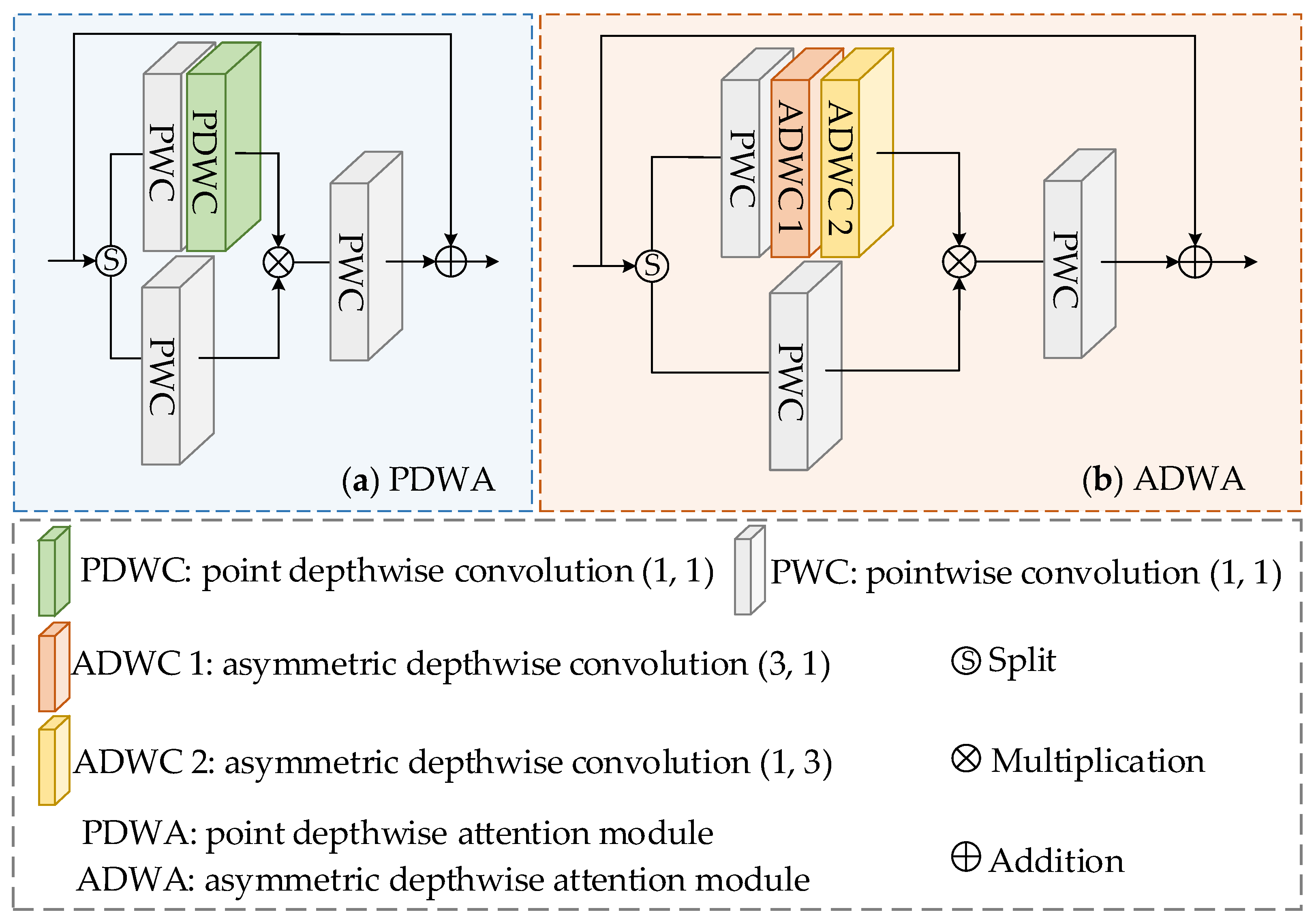
- A dual-branch fusion feature extraction module known as ASSF is developed in the study. The module contains the point depthwise attention module (PDWA) and the asymmetric depthwise attention module (ADWA). The PDWA primarily focuses on extracting spectral features from HSIs, whereas the ADWA is tailored to capture spatial information. The innovative design of ASSF enables the exclusion of linear layers, thereby accentuating local continuity while maintaining the richness of feature complexity.
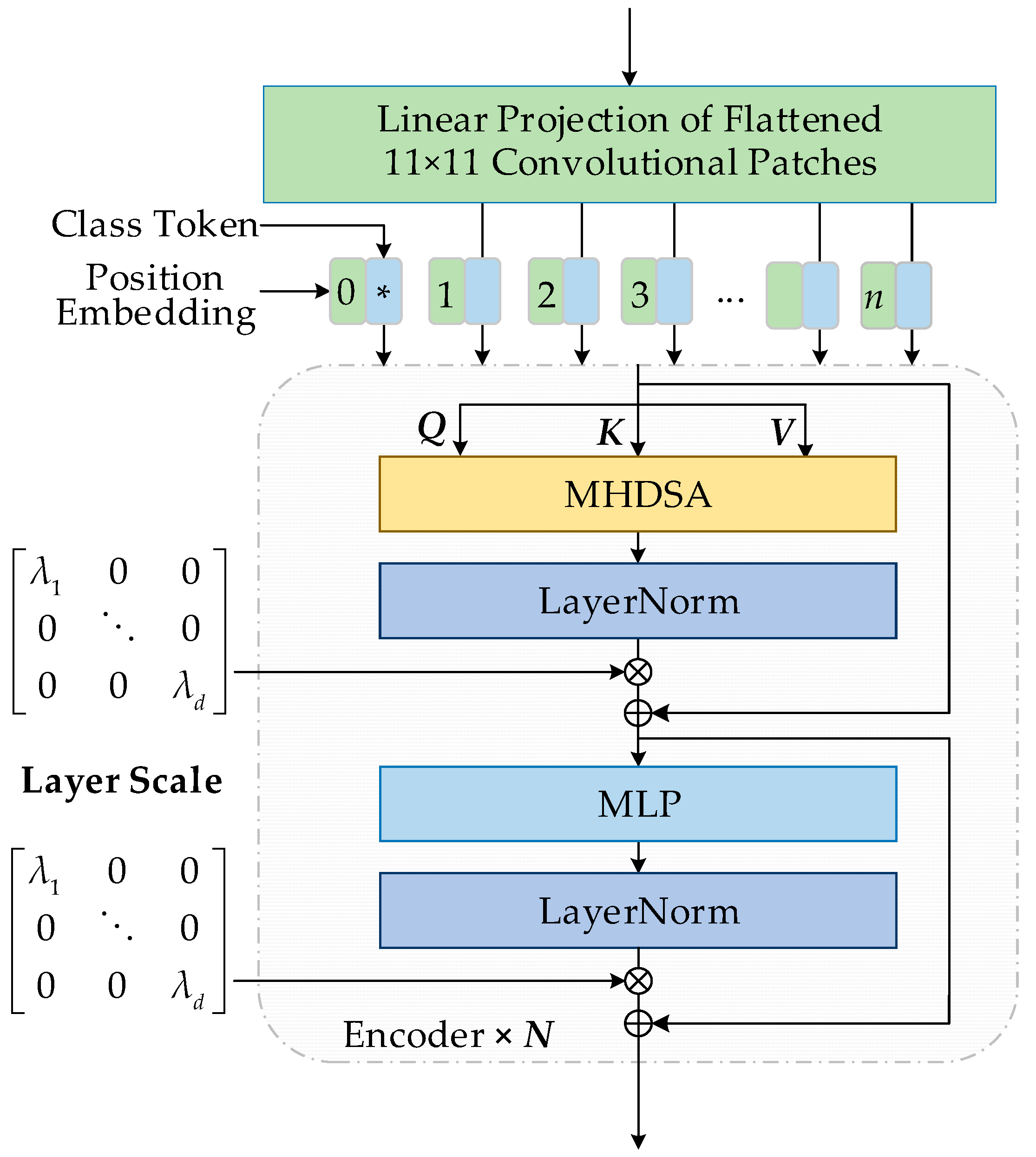
- The new transformer with a layer scale and DropKey (LD-Former) is proposed to increase the data dynamics and prevent performance degradation as the transformer deepens. The layer scale was added to the output of each residual block, and different output channels were multiplied by different values to make the features more refined. At the same time, the DropKey is adopted into self-attention (SA) to obtain DropKey self-attention (DSA). The combination of these two techniques overcomes the risk of overfitting and can train deeper transformers.
2. Methodology
2.1. Overall Architecture
2.2. Feature Extraction via ASSF
2.3. LD-Former Encoder
2.4. Final Classifier
| Algorithm 1 Adaptive Learnable Spectral–spatial Fusion Transformer for Hyperspectral Image Classification. | |
| Input: HSI: , Labels: , Patches = 11 × 11, PCA = 30. | |
| Output: Prediction: | |
| 1 | Initialize: batch size = 64, epochs = 100, the initial learning rate of the optimizer Adam depends on datasets. |
| 2 | PCA: . |
| 3 | Patches: Accomplish the slicing process for HSI to acquire the small patches . |
| 4 | Split and into training sets and test sets ( has the class labels, and has not the class labels). |
| 5 | Training ALSST (begin) |
| 6 | for epoch in range(epochs): |
| 7 | for i, (,) in enumerate (): |
| 8 | Generate the spectral–spatial fusion features using the ASSF. |
| 9 | Perform the LD-Former encoder: |
| 10 | The learnable class tokens are added to the first locations of the 1D spectral–spatial fusion feature vectors derived from ASSF, while the positional embedding is carried out to the total feature vectors, to form the semantic tokens. The semantic tokens learned by Equations (3)–(7). |
| 11 | Input the spectral–spatial class tokens from LD-Former into the MLP. |
| 12 | |
| 13 | |
| 14 | Training ALSST (end) and test ALSST |
| 15 | |
3. Experimental Results
3.1. Data Description
- TR dataset
- 2.
- MU dataset
- 3.
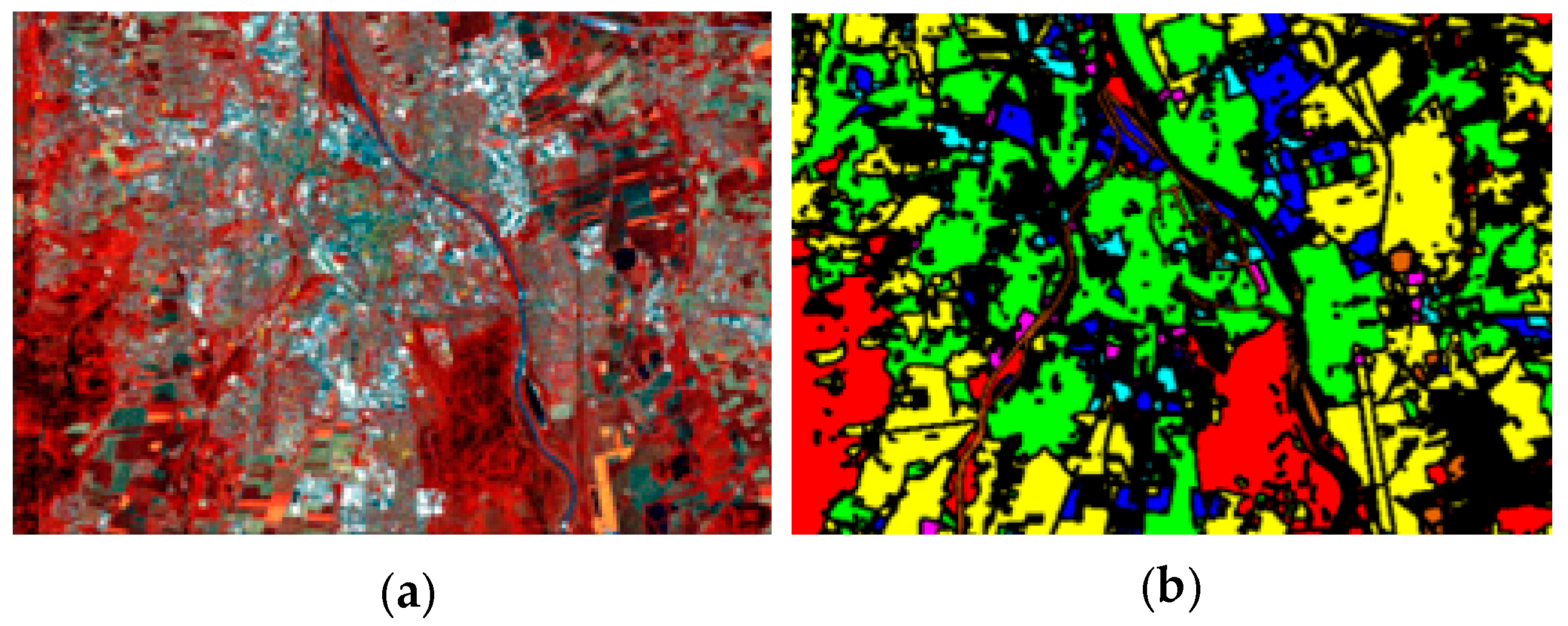
- AU dataset
- 4.
- UP dataset
3.2. Experimental Setting
3.2.1. Initial Learning Rate

| Datasets | Initial Learning Rate | ||
|---|---|---|---|
| 0.001 | 0.0005 | 0.0001 | |
| TR | 99.70 ± 0.03 | 99.68 ± 0.04 | 99.59 ± 0.01 |
| MU | 89.72 ± 0.36 | 88.67 ± 0.47 | 87.76 ± 0.69 |
| AU | 97.82 ± 0.11 | 97.84 ± 0.09 | 97.39 ± 0.04 |
| UP | 99.78 ± 0.03 | 99.56 ± 0.05 | 99.54 ± 0.06 |
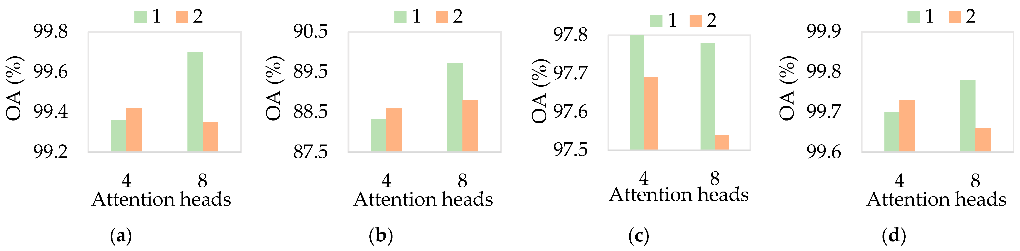
3.2.2. Depth and Heads
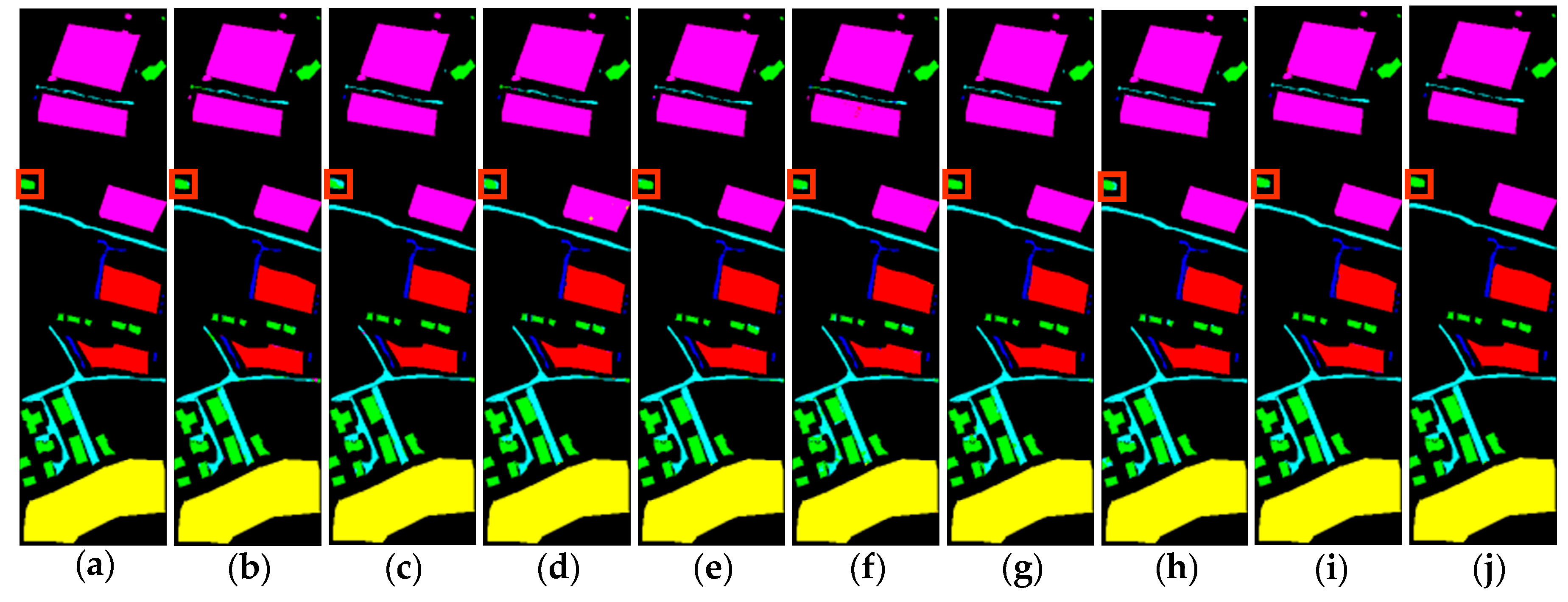
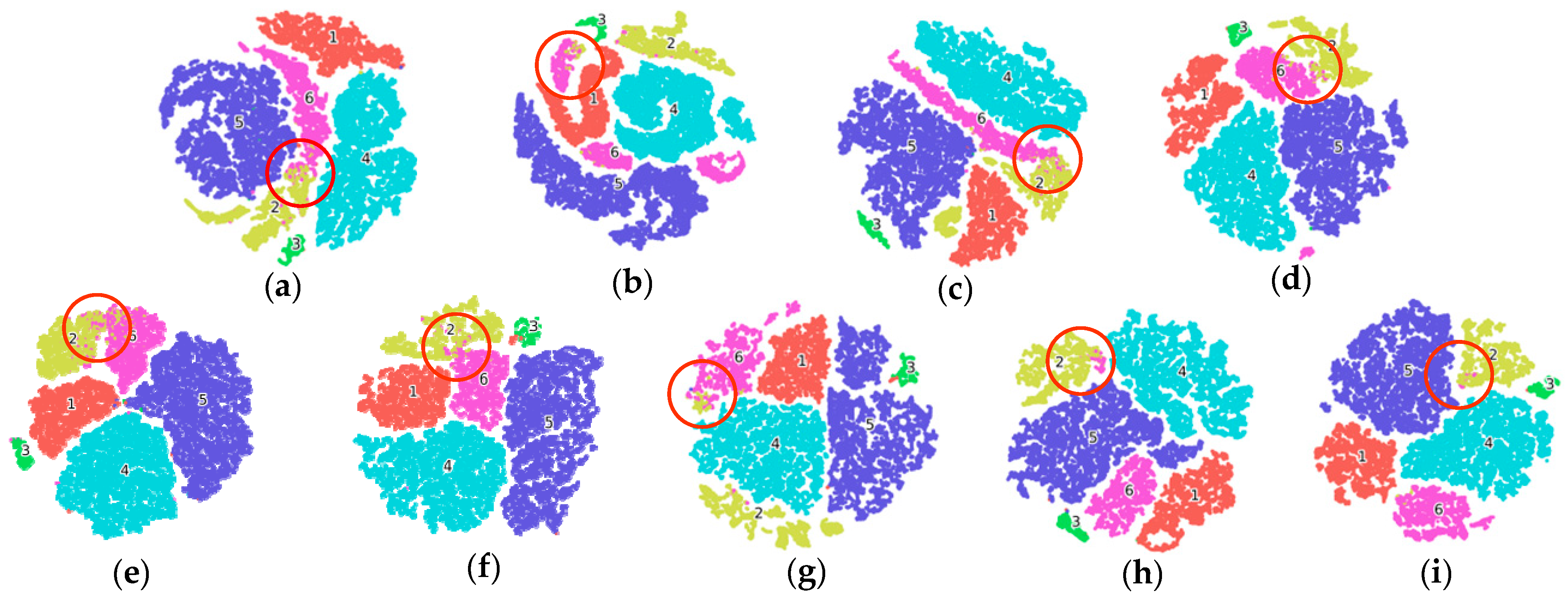
3.3. Performance Comparison
3.3.1. Experimental Results
- TR dataset
| Class | LiEtAl | SSRN | HyBridSN | DMCN | SpectralFormer | SSFTT | Morp- Former | 3D-ConvSST | ALSST |
|---|---|---|---|---|---|---|---|---|---|
| 1 | 99.39 ± 0.42 | 99.68 ± 0.23 | 99.23 ± 0.62 | 99.65 ± 0.35 | 99.10 ± 0.72 | 98.84 ± 0.61 | 97.89 ± 0.75 | 98.94± 0.39 | 99.56 ± 0.05 |
| 2 | 92.61 ± 1.47 | 94.31 ± 6.20 | 95.18 ± 2.08 | 99.74 ± 0.49 | 94.49 ± 0.39 | 98.01 ± 0.50 | 96.49 ± 2.57 | 99.06 ± 0.64 | 99.48 ± 0.25 |
| 3 | 97.75 ± 0.37 | 99.68 ± 0.64 | 99.89 ± 0.21 | 99.44 ± 0.56 | 97.54 ± 0.58 | 100 ± 0.00 | 100 ± 0.00 | 100 ± 0.00 | 100 ± 0.00 |
| 4 | 99.88 ± 0.12 | 99.99 ± 0.01 | 100 ± 0.00 | 99.99 ± 0.01 | 99.92 ± 0.08 | 100 ± 0.00 | 100 ± 0.00 | 100 ± 0.00 | 100 ± 0.00 |
| 5 | 99.62 ± 0.40 | 99.42 ± 1.07 | 99.24 ± 0.48 | 99.97 ± 0.03 | 99.65 ± 0.23 | 99.99 ± 0.01 | 99.97 ± 0.02 | 99.95 ± 0.05 | 100 ± 0.00 |
| 6 | 91.16 ± 2.99 | 97.06 ± 1.66 | 94.18 ± 1.58 | 96.42 ± 1.12 | 88.51 ± 5.55 | 95.38 ± 2.23 | 96.58 ± 2.84 | 98.39 ± 0.51 | 98.17 ± 0.23 |
| OA (%) | 98.10 ± 0.24 | 98.91 ± 0.55 | 98.57 ± 0.22 | 99.35 ± 0.17 | 97.99 ± 0.64 | 99.18 ± 0.12 | 99.02 ± 0.28 | 99.58 ± 0.08 | 99.70 ± 0.03 |
| AA (%) | 96.73 ± 0.41 | 98.36 ± 0.82 | 97.96 ± 0.26 | 98.87 ± 0.35 | 96.54 ± 0.51 | 98.70 ± 0.22 | 98.49 ± 0.42 | 99.39 ± 0.11 | 99.53 ± 0.05 |
| K × 100 | 97.46 ± 0.26 | 98.54 ± 0.74 | 98.09 ± 0.29 | 99.13 ± 0.58 | 97.31 ± 0.49 | 98.90 ± 0.17 | 98.69 ± 0.38 | 99.44 ± 0.11 | 99.60 ± 0.04 |
- 2.
- MU dataset
| Class | LiEtAl | SSRN | HyBridSN | DMCN | SpectralFormer | SSFTT | Morp- Former | 3D-ConvSST | ALSST |
|---|---|---|---|---|---|---|---|---|---|
| 1 | 85.06 ± 2.01 | 87.51 ± 1.37 | 84.03 ± 3.53 | 87.76 ± 2.37 | 88.62 ± 0.36 | 88.16 ± 0.57 | 85.14 ± 2.26 | 87.46 ± 0.89 | 89.65 ± 1.03 |
| 2 | 77.97 ± 3.56 | 83.77 ± 4.79 | 83.28 ± 2.45 | 84.85 ± 6.81 | 78.01 ± 9.75 | 84.27 ± 9.82 | 79.49 ± 6.40 | 81.75 ± 2.38 | 88.06 ± 1.17 |
| 3 | 74.57 ± 5.76 | 81.63 ± 3.24 | 79.96 ± 2.46 | 78.90 ± 3.35 | 81.75 ± 8.58 | 79.53 ± 3.86 | 81.83 ± 2.22 | 77.71 ± 4.43 | 86.21 ± 1.12 |
| 4 | 89.03 ± 4.60 | 95.27 ± 0.70 | 97.15 ± 1.16 | 96.42 ± 1.54 | 94.88 ± 2.49 | 93.89 ± 7.73 | 96.30 ± 0.65 | 94.62 ± 1.23 | 94.18 ± 1.85 |
| 5 | 81.11 ± 3.52 | 84.43 ± 1.04 | 82.14 ± 1.69 | 88.05 ± 3.91 | 88.62 ± 0.36 | 84.34 ± 3.17 | 79.83 ± 5.17 | 85.35 ± 2.31 | 87.77 ± 2.57 |
| 6 | 99.49 ± 0.51 | 100 ± 0.00 | 99.81 ± 0.25 | 99.84 ± 0.16 | 99.43 ± 0.57 | 99.68 ± 0.32 | 99.56 ± 0.38 | 99.24 ± 1.01 | 100 ± 0.00 |
| 7 | 87.48 ± 1.81 | 94.07 ± 0.95 | 90.06 ± 2.08 | 92.44 ± 3.04 | 91.38 ± 2.04 | 94.30 ± 2.57 | 90.16 ± 2.72 | 87.83 ± 2.07 | 95.59 ± 0.88 |
| 8 | 88.90 ± 4.96 | 91.64 ± 2.12 | 95.86 ± 1.27 | 94.56 ± 2.32 | 92.28 ± 0.85 | 93.03 ± 1.47 | 92.82 ± 2.00 | 93.76 ± 1.21 | 94.38 ± 0.55 |
| 9 | 64.96 ± 1.89 | 77.67 ± 2.34 | 76.99 ± 1.71 | 75.45 ± 3.57 | 76.79 ± 0.93 | 78.93 ± 1.39 | 76.16 ± 6.12 | 72.74 ± 1.40 | 83.45 ± 2.50 |
| 10 | 92.75 ± 4.21 | 99.39 ± 1.21 | 93.94 ± 3.31 | 94.24 ± 5.76 | 93.94 ± 6.06 | 86.68 ± 10.92 | 83.03 ± 10.43 | 90.30 ± 3.53 | 98.18 ± 1.48 |
| 11 | 97.14 ± 1.34 | 98.32 ± 0.92 | 98.99 ± 0.34 | 99.24 ± 0.76 | 99.50 ± 0.52 | 98.32 ± 1.68 | 98.99 ± 0.34 | 99.16 ± 0.03 | 98.82 ± 0.67 |
| OA (%) | 82.88 ± 2.30 | 86.94 ± 0.87 | 85.22 ± 1.47 | 87.39 ± 1.12 | 87.08 ± 1.24 | 87.06 ± 0.85 | 84.96 ± 1.10 | 86.21 ± 0.70 | 89.72 ± 0.36 |
| AA (%) | 85.13 ± 1.20 | 90.34 ± 0.49 | 89.29 ± 0.62 | 90.09 ± 0.99 | 89.30 ± 1.12 | 89.18 ± 1.64 | 87.57 ± 0.80 | 88.17 ± 0.53 | 92.39 ± 0.51 |
| K × 100 | 77.86 ± 0.93 | 83.05 ± 1.08 | 80.97 ± 1.75 | 83.60 ± 0.21 | 83.14 ± 1.64 | 83.19 ± 0.43 | 80.61 ± 1.31 | 82.12 ± 0.87 | 86.59 ± 0.46 |
- 3.
- AU dataset
| Class | LiEtAl | SSRN | HyBridSN | DMCN | SpectralFormer | SSFTT | Morp- Former | 3D-ConvSST | ALSST |
|---|---|---|---|---|---|---|---|---|---|
| 1 | 98.25 ± 0.43 | 98.94 ± 0.22 | 99.12 ± 0.26 | 98.59 ± 0.56 | 86.10 ± 0.44 | 98.82 ± 0.08 | 97.71 ± 0.21 | 99.09 ± 0.32 | 98.67 ± 0.25 |
| 2 | 77.97 ± 3.56 | 99.23 ± 0.25 | 99.16 ± 0.36 | 98.52 ± 0.44 | 96.10 ± 1.44 | 99.02 ± 0.33 | 98.54 ± 0.25 | 98.58 ± 0.25 | 99.06 ± 0.09 |
| 3 | 97.54 ± 0.48 | 89.29 ± 1.18 | 95.61 ± 1.00 | 87.64 ± 1.51 | 75.99 ± 8.92 | 90.13 ± 1.39 | 89.69 ± 1.46 | 93.33 ± 1.53 | 95.96 ± 0.39 |
| 4 | 98.54 ± 0.22 | 99.12 ± 0.22 | 98.95 ± 0.21 | 99.02 ± 0.58 | 98.66 ± 0.34 | 98.77 ± 0.34 | 98.53 ± 0.11 | 98.86 ± 0.18 | 99.13 ± 0.14 |
| 5 | 64.97 ± 5.04 | 85.01 ± 5.23 | 84.64 ± 9.87 | 71.08 ± 3.99 | 48.88 ± 7.61 | 79.09 ± 5.60 | 84.88 ± 3.06 | 81.02 ± 2.98 | 87.39 ± 4.08 |
| 6 | 46.60 ± 2.01 | 69.67 ± 4.19 | 72.04 ± 3.59 | 47.82 ± 5.15 | 27.56 ± 9.54 | 70.12 ± 3.37 | 75.45 ± 3.58 | 64.48 ± 2.90 | 78.80 ± 1.73 |
| 7 | 58.39 ± 3.58 | 72.93 ± 2.74 | 72.67 ± 1.95 | 64.51 ± 1.86 | 55.50 ± 4.95 | 66.88 ± 1.20 | 71.36 ± 3.58 | 71.90 ± 2.29 | 73.08 ± 0.60 |
| OA (%) | 94.84 ± 0.39 | 97.41 ± 0.24 | 96.50 ± 0.08 | 96.24 ± 1.36 | 93.89 ± 0.27 | 97.08 ± 0.18 | 96.85 ± 0.07 | 97.14 ± 0.18 | 97.84 ± 0.09 |
| AA (%) | 71.66 ± 0.85 | 87.74 ± 1.59 | 84.44 ± 0.58 | 81.03 ± 2.30 | 71.66 ± 2.58 | 86.12 ± 1.93 | 88.03 ± 1.21 | 86.75 ± 1.02 | 90.30 ± 0.71 |
| K × 100 | 92.58 ± 0.79 | 96.29 ± 0.34 | 94.98 ± 0.11 | 94.60 ± 0.42 | 91.22 ± 0.43 | 95.81 ± 0.25 | 95.48 ± 0.10 | 95.90 ± 0.26 | 96.91 ± 0.13 |
- 4.
- UP dataset
| Class | LiEtAl | SSRN | HyBridSN | DMCN | SpectralFormer | SSFTT | Morp- Former | 3D-ConvSST | ALSST |
|---|---|---|---|---|---|---|---|---|---|
| 1 | 99.06 ± 0.4 | 99.8 ± 0.08 | 98.22 ± 0.31 | 99.70 ± 0.14 | 97.54 ± 0.18 | 99.73 ± 0.29 | 99.65 ± 0.10 | 99.81 ± 0.17 | 99.99 ± 0.01 |
| 2 | 99.76 ± 0.10 | 99.99 ± 0.03 | 99.95 ± 0.04 | 99.95 ± 0.05 | 99.89 ± 0.09 | 99.97± 0.02 | 99.97 ± 0.03 | 99.97 ± 0.02 | 99.99 ± 0.01 |
| 3 | 86.53 ± 1.52 | 97.07 ± 1.93 | 93.24 ± 1.30 | 94.78 ± 2.55 | 85.79 ± 2.05 | 97.39 ± 0.87 | 98.06 ± 1.38 | 97.55 ± 1.04 | 99.91 ± 0.11 |
| 4 | 95.49 ± 0.54 | 99.31 ± 0.41 | 98.43 ± 0.38 | 97.20 ± 1.20 | 97.45 ± 0.74 | 97.95 ± 0.64 | 98.34 ± 0.39 | 97.98 ± 0.47 | 98.17 ± 0.35 |
| 5 | 100 ± 0.00 | 99.95 ± 0.09 | 100 ± 0.00 | 100 ± 0.00 | 99.98 ± 0.03 | 99.94 ± 0.09 | 99.55 ± 0.27 | 100 ± 0.00 | 99.97 ± 0.04 |
| 6 | 97.56 ± 0.65 | 100 ± 0.00 | 97.70 ± 0.29 | 99.89 ± 0.15 | 99.31 ± 0.47 | 99.75 ± 0.29 | 99.99 ± 0.02 | 100 ± 0.00 | 99.98 ± 0.04 |
| 7 | 98.86 ± 1.18 | 98.53 ± 0.55 | 99.41 ± 0.4 | 99.49 ± 0.38 | 99.43 ± 0.24 | 99.90 ± 0.19 | 99.79 ± 0.14 | 99.95 ± 0.06 | 100 ± 0.00 |
| 8 | 94.60 ± 1.03 | 98.07 ± 0.43 | 94.90 ± 1.00 | 97.40 ± 1.00 | 94.36 ± 1.28 | 98.30 ± 0.72 | 95.91 ± 0.91 | 98.75 ± 0.31 | 99.50 ± 0.23 |
| 9 | 94.58 ± 3.34 | 100 ± 0.00 | 97.98 ± 0.73 | 98.89 ± 1.22 | 95.62 ± 2.01 | 98.71 ± 0.51 | 96.24 ± 0.60 | 96.98 ± 0.57 | 98.62 ± 0.45 |
| OA (%) | 97.86 ± 0.39 | 99.56 ± 0.09 | 98.49 ± 0.16 | 99.20 ± 0.13 | 98.01 ± 0.11 | 99.46 ± 0.15 | 99.26 ± 0.05 | 99.52 ± 0.06 | 99.78 ± 0.03 |
| AA (%) | 96.27 ± 0.74 | 99.20 ± 0.19 | 97.76 ± 0.32 | 98.59 ± 0.24 | 96.60 ± 0.24 | 99.07 ± 0.25 | 98.61 ± 0.15 | 99.00 ± 0.13 | 99.57 ± 0.08 |
| K × 100 | 97.16 ± 0.52 | 99.42 ± 0.12 | 97.99 ± 0.21 | 98.94 ± 0.17 | 97.36 ± 0.15 | 99.29 ± 0.20 | 99.02 ± 0.07 | 99.36 ± 0.08 | 99.71 ± 0.04 |
3.3.2. Consumption and Computational Complexity
4. Discussion
4.1. Ablation Analysis
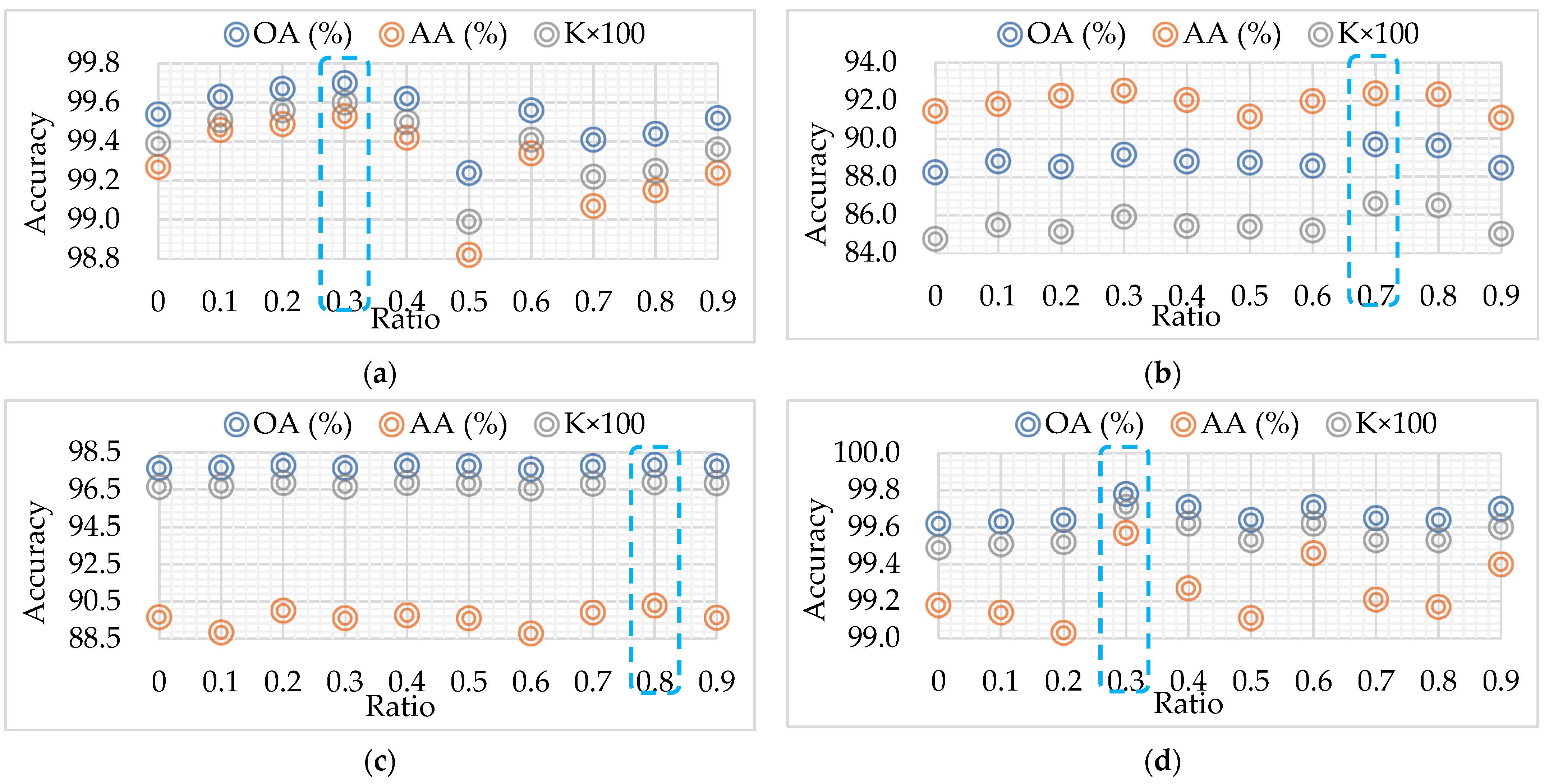
4.2. Ratio of DropKey
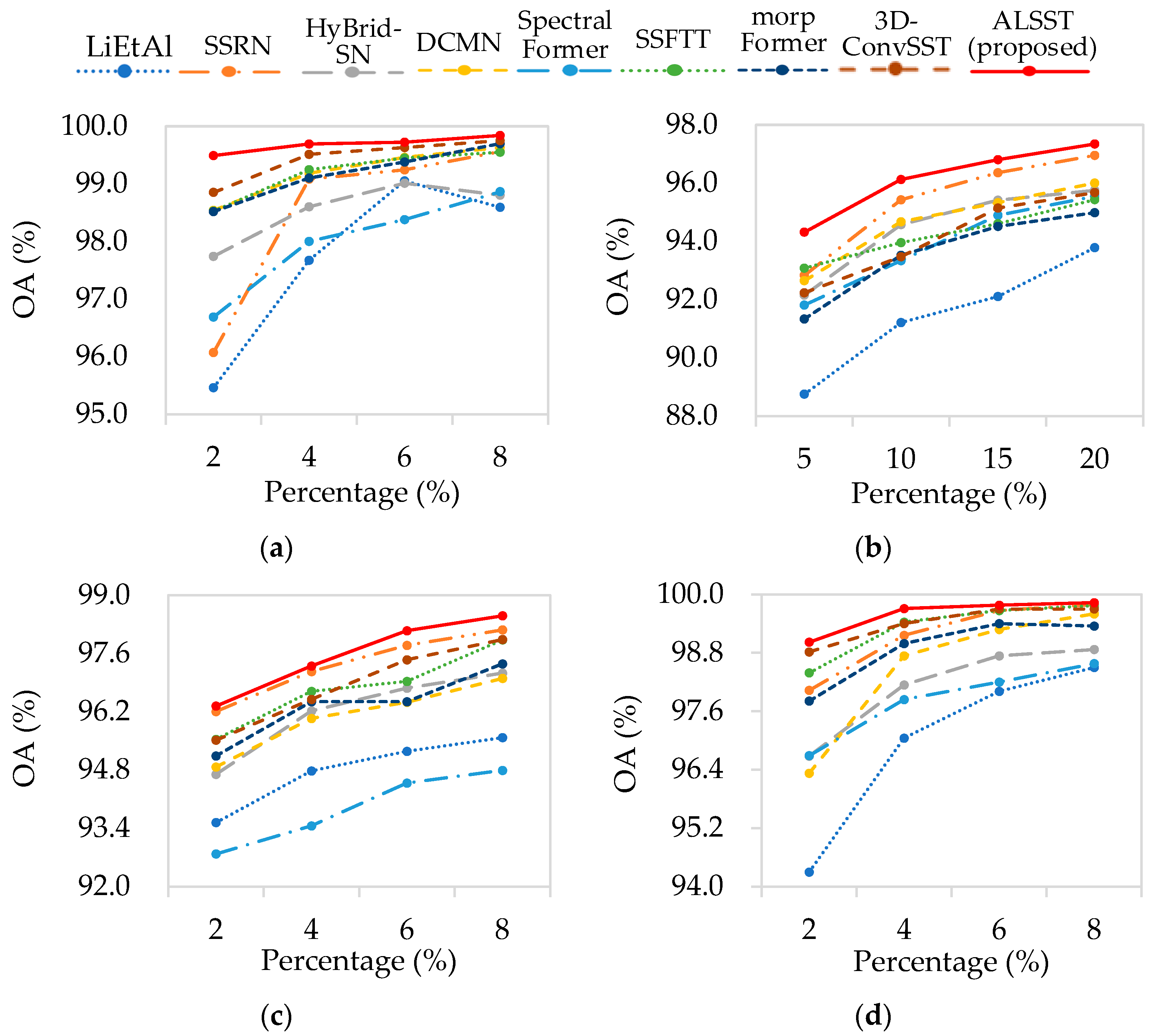
4.3. Training Percentage
5. Conclusions
Author Contributions
Funding
Data Availability Statement
Acknowledgments
Conflicts of Interest
References
- Czaja, W.; Kavalerov, I.; Li, W. Exploring the High Dimensional Geometry of HSI Features. In Proceedings of the 2021 11th Workshop on Hyperspectral Imaging and Signal Processing: Evolution in Remote Sensing (WHISPERS), Amsterdam, The Netherlands, 24–26 March 2021; pp. 1–5. [Google Scholar]
- Mahlein, A.; Oerke, E.; Steiner, U.; Dehne, H. Recent Advances in Sensing Plant Diseases for Precision Crop Protection. Eur. J. Plant Pathol. 2012, 133, 197–209. [Google Scholar] [CrossRef]
- Shimoni, M.; Haelterman, R.; Perneel, C. Hyperspectral imaging for military and security applications: Combining myriad processing and sensing techniques. IEEE Geosci. Remote Sens. Mag. 2019, 7, 101–117. [Google Scholar] [CrossRef]
- Hestir, E.; Brando, V.; Bresciani, M.; Giardino, C.; Matta, E.; Villa, P.; Dekker, A. Measuring Freshwater Aquatic Ecosystems: The Need for a Hyperspectral Global Mapping Satellite Mission. Remote Sens. Environ. 2015, 167, 181–195. [Google Scholar] [CrossRef]
- Xu, Y.; Du, B.; Zhang, F.; Zhang, L. Hyperspectral Image Classification Via a Random Patches Network. ISPRS J. Photogramm. Remote Sens. 2018, 142, 344–357. [Google Scholar] [CrossRef]
- Wu, X.; Hong, D.; Chanussot, J. UIU-Net: U-Net in U-Net for infrared small object detection. IEEE Trans. Image Process. 2023, 32, 364–376. [Google Scholar] [CrossRef] [PubMed]
- Vaishnavi, B.B.S.; Pamidighantam, A.; Hema, A.; Syam, V.R. Hyperspectral Image Classification for Agricultural Applications. In Proceedings of the IEEE 2022 International Conference on Electronics and Renewable Systems (ICEARS), Tuticorin, India, 16–18 March 2022; pp. 1–7. [Google Scholar]
- Schimleck, L.; Ma, T.; Inagaki, T.; Tsuchikawa, S. Review of Near Infrared Hyperspectral Imaging Applications Related to Wood and Wood Products. Appl. Spectrosc. Rev. 2022, 57, 2098759. [Google Scholar] [CrossRef]
- Liao, X.; Liao, G.; Xiao, L. Rapeseed Storage Quality Detection Using Hyperspectral Image Technology–An Application for Future Smart Cities. J. Test. Eval. 2022, 51, JTE20220073. [Google Scholar] [CrossRef]
- Xiang, J.H.; Wei, C.; Wang, M.H.; Teng, L. End-to-End Multilevel Hybrid Attention Framework for Hyperspectral Image Classification. IEEE Geosci. Remote Sens. Let. 2022, 19, 5511305. [Google Scholar] [CrossRef]
- Feng, J.; Bai, G.; Li, D.; Zhang, X.G.; Shang, R.H.; Jiao, L.C. MR-Selection: A Meta-Reinforcement Learning Approach for Zero-Shot Hyperspectral Band Selection. IEEE Trans. Geosci. Remote Sens. 2022, 61, 5500320. [Google Scholar] [CrossRef]
- Ma, X.; Zhang, X.; Tang, X.; Zhou, H.; Jiao, L. Hyperspectral Anomaly Detection Based on Low-Rank Representation with DataDriven Projection and Dictionary Construction. IEEE J. Sel. Top. Appl. Earth Obs. Remote Sens. 2020, 13, 2226–2239. [Google Scholar] [CrossRef]
- Hong, D.; Wu, X.; Ghamisi, P.; Chanussot, J.; Yokoya, N.; Zhu, X.X. Invariant attribute profiles: A Spatial-Frequency Joint Feature Extractor for Hyperspectral Image Classification. IEEE Trans. Geosci. Remote Sens. 2020, 58, 3791–3808. [Google Scholar] [CrossRef]
- Bruzzone, L.; Roli, F.; Serpico, S.B. An Extension of the Ieffreys–Matusita Distance to Multiclasscases for Feature Selection. IEEE Tran. Geosci. Remote Sens. 1995, 33, 1318–1321. [Google Scholar] [CrossRef]
- Keshava, N. Distance Metrics and Band Selection in Hyperspectral Processing with Applications to Material Identification and Spectral Libraries. IEEE Trans. Geosci. Remote Sens. 2004, 42, 1552–1565. [Google Scholar] [CrossRef]
- Prasad, S.; Bruce, L.M. Limitations of Principal Components Analysis for Hyperspectral Target Recognition. IEEE Geosci. Remote Sens. Let. 2008, 5, 625–629. [Google Scholar] [CrossRef]
- Villa, A.; Benediktsson, J.A.; Chanussot, J. Hyperspectral Image Classification with Independent Component Discriminant Analysis. IEEE Geosci. Remote Sens. 2011, 49, 4865–4876. [Google Scholar] [CrossRef]
- Bandos, T.V.; Bruzzone, L.; Camps–Valls, G. Classification of Hyperspectral Images with Regularized Linear Discriminant Analysis. IEEE Geosci. Remote Sens. 2009, 47, 862–873. [Google Scholar] [CrossRef]
- Friedl, M.A.; Brodley, C.E. Decision Tree Classification of Land Cover from Remotely Sensed Data. Remote Sens. Environ. 1997, 61, 399–409. [Google Scholar] [CrossRef]
- Melgani, F.; Bruzzone, L. Classification of Hyperspectral Remote Sensing Images with Support Vector Machines. IEEE Geosci. Remote Sens. 2004, 42, 1778–1790. [Google Scholar] [CrossRef]
- Blanzieri, E.; Melgani, F. Nearest Neighbor Classification of Remote Sensing Images with the Maximal Margin Principle. IEEE Geosci. Remote Sens. 2008, 46, 1804–1811. [Google Scholar] [CrossRef]
- Lu, Y.; Wang, L.; Shi, Y. Classification of Hyperspectral Image with Small-Sized Samples Based on Spatial–Spectral Feature Enhancement. J. Harbin Eng. Univ. 2022, 43, 436–443. [Google Scholar]
- Zhang, R.; Xu, L.; Yu, Z.; Shi, Y.; Mu, C.; Xu, M. Deep-IRTarget: An automatic target detector in infrared imagery using dual-domain feature extraction and allocation. IEEE Trans. Multimed. 2022, 24, 1735–1749. [Google Scholar] [CrossRef]
- Zhang, R.; Cao, Z.; Yang, S.; Si, L.; Sun, H.; Xu, L.; Sun, F. Cognition-Driven Structural Prior for Instance-Dependent Label Transition Matrix Estimation. IEEE Trans. Neural Netw. Learn. Syst. 2024, 35, 38190682. [Google Scholar] [CrossRef] [PubMed]
- Zhang, R.; Tan, J.; Cao, Z.; Xu, L.; Liu, Y.; Si, L.; Sun, F. Part-Aware Correlation Networks for Few-shot Learning. IEEE Trans. Multimedia. 2024, 1–13. [Google Scholar] [CrossRef]
- Zhang, R.; Yang, S.; Zhang, Q.; Xu, L.; He, Y.; Zhang, F. Graph-based few-shot learning with transformed feature propagation and optimal class allocation. Neuro Comput. 2022, 470, 247–256. [Google Scholar] [CrossRef]
- Hong, Q.Q.; Zhong, X.Y.; Chen, W.T.; Zhang, Z.G.; Li, B. SATNet: A Spatial Attention Based Network for Hyperspectral Image Classification. Remote Sens. 2022, 14, 5902. [Google Scholar] [CrossRef]
- Chen, Y.; Lin, Z.; Zhao, X.; Wang, G.; Gu, Y. Deep Learning-Based Classification of Hyperspectral Data. IEEE J. Sel. Top. Appl. Earth Obs. Remote Sens. 2014, 7, 2094–2107. [Google Scholar] [CrossRef]
- Chen, Y.; Zhao, X.; Jia, X. Spectral–Spatial Classification of Hyperspectral Data Based on Deep Belief Network. IEEE J. Sel. Top. Appl. Earth Obs. Remote Sens. 2015, 8, 2381–2392. [Google Scholar] [CrossRef]
- Chen, Y.; Jiang, H.; Li, C.; Jia, X.; Ghamisi, P. Deep Feature Extraction and Classification of Hyperspectral Images Based on Convolutional Neural Networks. IEEE Trans. Geosci. Remote Sens. 2016, 54, 6232–6251. [Google Scholar] [CrossRef]
- Hong, D.; Gao, L.; Yao, J.; Zhang, B.; Plaza, A.; Chanussot, J. Graph Convolutional Networks for Hyperspectral Image Classification. IEEE Trans. Geosci. Remote Sens. 2020, 59, 5966–5978. [Google Scholar] [CrossRef]
- He, X.; Chen, Y.; Li, Q. Two-Branch Pure Transformer for Hyperspectral Image Classification. IEEE Geosci. Remote Sens. Lett. 2022, 19, 6015005. [Google Scholar] [CrossRef]
- Zhu, K.; Chen, Y.; Ghamisi, P.; Jia, X.; Benediktsson, J.A. Deep Convolutional Capsule Network for Hyperspectral Image Spectral and Spectral-Spatial Classification. Remote Sens. 2019, 11, 223. [Google Scholar] [CrossRef]
- Feng, J.; Yu, H.; Wang, L.; Cao, X.; Zhang, X.; Jiao, L. Classification of Hyperspectral Images Based on Multiclass Spatial–Spectral Generative Adversarial Networks. IEEE Trans. Geosci. Remote Sens. 2019, 57, 5329–5343. [Google Scholar] [CrossRef]
- Roy, S.K.; Krishna, G.; Dubey, S.R.; Chaudhuri, B.B. HybridSN: Exploring 3-D–2-D CNN feature hierarchy for hyperspectral image classification. IEEE Geosci. Remote Sens. Lett. 2020, 17, 277–281. [Google Scholar] [CrossRef]
- Sun, Y.; Wang, M.; Wei, C.; Zhong, Y.; Xiang, J. Heterogeneous spectral-spatial network with 3D attention and MLP for hyperspectral image classification using limited training samples. IEEE J. Sel. Top. Appl. Earth Obs. Remote Sens. 2023, 16, 8702–8720. [Google Scholar] [CrossRef]
- Hong, D.; Han, Z.; Yao, J. SpectralFormer: Rethinking hyperspectral image classification with transformers. IEEE Trans. Geosci. Remote Sens. 2022, 60, 5518615. [Google Scholar] [CrossRef]
- Sun, L.; Zhao, G.; Zheng, Y.; Wu, Z. Spectral–spatial feature tokenization transformer for hyperspectral image classification. IEEE Trans. Geosci. Remote Sens. 2022, 60, 1–14. [Google Scholar] [CrossRef]
- Wang, A.; Xing, S.; Zhao, Y.; Wu, H.; Iwahori, Y. A hyperspectral image classification method based on adaptive spectral spatial kernel combined with improved vision transformer. Remote Sens. 2022, 14, 3705. [Google Scholar] [CrossRef]
- Huang, X.; Dong, M.; Li, J.; Guo, X. A 3-d-swin transformer-based hierarchical contrastive learning method for hyperspectral image classification. IEEE Trans. Geosci. Remote Sens. 2022, 60, 5411415. [Google Scholar] [CrossRef]
- Fang, Y.; Ye, Q.; Sun, L.; Zheng, Y.; Wu, Z. Multi-attention joint convolution feature representation with lightweight transformer for hyperspectral image classification. IEEE Trans. Geosci. Remote Sens. 2023, 61, 5513814. [Google Scholar] [CrossRef]
- Gulati, A.; Qin, J.; Chiu, C.C. Conformer: Convolution-augmented transformer for speech recognition. arXiv 2020, arXiv:2005.08100. [Google Scholar]
- Wang, Y.; Li, Y.; Wang, G.; Liu, X. Multi-scale attention network for single image super-resolution. arXiv 2022, arXiv:2209.14145. [Google Scholar]
- Hendrycks, D.; Gimpel, K. Gaussian Error Linear Units (gelus). arXiv 2016, arXiv:1606.08415. [Google Scholar]
- Touvron, H.; Cord, M.; Sablayrolles, A. Going deeper with image transformers. arXiv 2021, arXiv:2103.17239v2. [Google Scholar]
- Li, B.; Hu, Y.; Nie, X.; Han, C.; Jiang, X.; Guo, T.; Liu, L. DropKey. arXiv 2023, arXiv:2208.02646v4. [Google Scholar]
- Gader, P.; Zare, A.; Close, R.; Aitken, J.; Tuell, G. Muufl Gulfport Hyperspectral and LiDAR Airborne Data Set; Technical Report REP-2013–570; University of Florida: Gainesville, FL, USA, 2013. [Google Scholar]
- Du, X.; Zare, A. Scene Label Ground T ruth Map for Muufl Gulfport Data Set; Technical Report 20170417; University of Florida: Gainesville, FL, USA, 2017. [Google Scholar]
- Li, Y.; Zhang, H.K.; Shen, Q. Spectral–Spatial Classification of Hyperspectral Imagery with 3D Convolutional Neural Network. Remote Sens. 2017, 9, 67. [Google Scholar] [CrossRef]
- Zhong, Z.; Li, J.; Luo, Z.; Chapman, M. Spectral–Spatial Residual Network for Hyperspectral Image Classification: A 3-D Deep Learning Framework. IEEE Trans. Geosci. Remote Sens. 2018, 56, 847–858. [Google Scholar] [CrossRef]
- Swalpa, K.R.; Ankur, D.; Shah, C. Spectral–spatial morphological attention transformer for hyperspectral image classification. IEEE Trans. Geosci. Remote Sens. 2022, 61, 5503615. [Google Scholar]
- Shyam, V.; Aryaman, S.; Shiv, R.D.; Satish, K.S. 3D-Convolution Guided Spectral-Spatial Transformer for Hyperspectral Image Classification. arXiv 2024, arXiv:2404.13252. [Google Scholar]


| No. | Color | Class Name | Training Samples | Test Samples |
|---|---|---|---|---|
| 1 |  | Apple Trees | 129 | 3905 |
| 2 | Buildings | 125 | 2778 | |
| 3 | Ground | 105 | 374 | |
| 4 | Woods | 154 | 9896 | |
| 5 | Vineyard | 184 | 10,317 | |
| 6 | Roads | 122 | 3052 | |
| Total | 819 | 29,395 | ||
| No. | Color | Class Name | Training Samples | Test Samples |
|---|---|---|---|---|
| 1 |  | Trees | 150 | 23,096 |
| 2 | Mostly Grass | 150 | 4120 | |
| 3 | Mixed Ground Surface | 150 | 6732 | |
| 4 | Dirt and Sand | 150 | 1676 | |
| 5 | Road | 150 | 6537 | |
| 6 | Water | 150 | 316 | |
| 7 | Buildings Shadow | 150 | 2083 | |
| 8 | Buildings | 150 | 6090 | |
| 9 | Sidewalk | 150 | 1235 | |
| 10 | Yellow Curb | 150 | 33 | |
| 11 | Cloth Panels | 150 | 119 | |
| Total | 1650 | 52,037 | ||
| No. | Color | Class Name | Training Samples | Test Samples |
|---|---|---|---|---|
| 1 |  | Forest | 675 | 12,832 |
| 2 | Residential Area | 1516 | 28,813 | |
| 3 | Industrial Area | 192 | 3659 | |
| 4 | Low Plants | 1342 | 25,515 | |
| 5 | Allotment | 28 | 547 | |
| 6 | Commercial Area | 82 | 1563 | |
| 7 | Water | 16 | 1454 | |
| Total | 3911 | 74,383 | ||
| No. | Color | Class Name | Training Samples | Test Samples |
|---|---|---|---|---|
| 1 |  | Asphalt | 332 | 6299 |
| 2 | Meadows | 932 | 17,717 | |
| 3 | Gravel | 105 | 1994 | |
| 4 | Trees | 153 | 2911 | |
| 5 | Metal sheets | 67 | 1278 | |
| 6 | Bare soil | 251 | 4778 | |
| 7 | Bitumen | 67 | 1263 | |
| 8 | Bricks | 184 | 3498 | |
| 9 | Shadow | 47 | 900 | |
| Total | 2138 | 40,638 | ||
| Methods | TPs | Tr (s) | Te (s) | Flops | OA (%) | TPs | Tr (s) | Te (s) | Flops | OA (%) |
| TR | MU | |||||||||
| LiEtAl | 36.64 K | 4.56 | 0.35 | 40.21 M | 98.10 ± 0.24 | 66.89 K | 6.85 | 0.56 | 42.14 M | 82.88 ± 2.30 |
| SSRN | 102.80 K | 11.76 | 0.89 | 2.102 G | 98.91 ± 0.55 | 102.92 K | 22.72 | 1.62 | 2.10 G | 86.94 ± 0.87 |
| HyBridSN | 1.52 M | 5.23 | 0.55 | 416.79 M | 98.57 ± 0.22 | 1.15 M | 9.41 | 0.92 | 416.83 M | 85.22 ± 1.47 |
| DMCN | 2.77 M | 20.22 | 1.69 | 3.21 G | 99.35 ± 0.17 | 2.77 M | 34.40 | 3.04 | 3.21 G | 87.39 ± 1.12 |
| SpectralFormer | 97.33 K | 46.80 | 3.55 | 192.68 M | 97.99 ± 0.64 | 97.65 K | 93.22 | 6.22 | 192.70 M | 87.08 ± 1.24 |
| SSFTT | 147.84 K | 22.08 | 1.51 | 447.18 M | 99.18 ± 0.12 | 148.16 K | 38.06 | 2.78 | 447.20 M | 87.06 ± 0.85 |
| morpFormer | 62.56 K | 38.36 | 4.38 | 334.43 M | 99.02 ± 0.28 | 62.56 K | 77.67 | 7.11 | 334.43 M | 84.96 ± 1.10 |
| 3D-ConvSST | 499.04 K | 33.47 | 3.03 | 7.95 G | 99.58 ± 0.08 | 499.37 K | 66.44 | 5.36 | 7.95 G | 86.21 ± 0.70 |
| ALSST | 157.06 K | 40.90 | 3.78 | 1.53 G | 99.70 ± 0.03 | 157.39 K | 38.70 | 3.14 | 1.53 G | 89.72 ± 0.36 |
| Methods | AU | UP | ||||||||
| LiEtAl | 42.69 K | 12.95 | 0.84 | 40.59 M | 94.84 ± 0.39 | 54.79 K | 7.21 | 0.52 | 41.37 M | 97.86 ± 0.39 |
| SSRN | 102.82 K | 54.83 | 2.48 | 2.10 G | 97.41 ± 0.24 | 102.87 K | 33.10 | 1.48 | 2.10 G | 99.56 ± 0.09 |
| HyBridSN | 1.15 M | 17.94 | 1.05 | 416.80 M | 96.50 ± 0.08 | 1.15 M | 10.02 | 0.57 | 416.81 M | 98.49 ± 0.16 |
| DMCN | 2.77 M | 76.96 | 3.82 | 3.21 G | 96.24 ± 1.36 | 2.77 M | 42.02 | 2.19 | 3.21 G | 99.20 ± 0.13 |
| SpectralFormer | 97.39 K | 202.32 | 8.03 | 192.68 M | 93.89 ± 0.27 | 97.52 K | 41.34 | 2.17 | 192.69 M | 98.01 ± 0.11 |
| SSFTT | 147.90 K | 93.01 | 3.97 | 447.18 M | 97.08 ± 0.18 | 148.03 K | 19.84 | 1.15 | 447.19 M | 99.46 ± 0.15 |
| morpFormer | 62.56 K | 185.38 | 10.22 | 334.43 M | 96.85 ± 0.07 | 62.56 K | 102.12 | 6.46 | 334.43 M | 99.26 ± 0.05 |
| 3D-ConvSST | 499.11 K | 155.33 | 7.93 | 7.95 G | 97.14 ± 0.18 | 499.24 K | 85.22 | 4.28 | 7.95 G | 99.52 ± 0.06 |
| ALSST | 157.13 K | 66.45 | 3.18 | 1.53 G | 97.84 ± 0.09 | 157.26 K | 45.50 | 2.17 | 1.53 G | 99.78 ± 0.03 |
| PDWA | ADWA | TE | LD-Former | OA (%) | AA (%) | K × 100 | ||
|---|---|---|---|---|---|---|---|---|
| Layer Scale | DropKey | |||||||
| √ | √ | √ | 78.06 ± 1.05 | 63.62 ± 1.05 | 70.43 ± 1.31 | |||
| √ | √ | √ | √ | 99.53 ± 0.05 | 99.06 ± 0.09 | 99.38 ± 0.07 | ||
| √ | √ | 99.57 ± 0.04 | 99.11 ± 0.11 | 99.44 ± 0.06 | ||||
| √ | √ | √ | √ | 99.73 ± 0.02 | 99.47 ± 0.05 | 99.64 ± 0.03 | ||
| √ | √ | √ | √ | 99.52 ± 0.04 | 98.99 ± 0.07 | 99.37 ± 0.05 | ||
| √ | √ | √ | √ | 99.51 ± 0.05 | 99.10 ± 0.06 | 99.35 ± 0.06 | ||
| √ | √ | √ | √ | 99.56 ± 0.21 | 99.12 ± 0.29 | 99.42 ± 0.27 | ||
| √ | √ | √ | √ | 99.65 ± 0.27 | 99.44 ± 0.33 | 99.53 ± 0.36 | ||
| √ | √ | √ | √ | √ | 99.78 ± 0.03 | 99.57 ± 0.08 | 99.71 ± 0.04 | |
| Kernel Size | OA (%) | AA (%) | K × 100 |
|---|---|---|---|
| 99.57 ± 0.05 | 99.12 ± 0.09 | 99.43 ± 0.06 | |
| and | 99.78 ± 0.03 | 99.57 ± 0.08 | 99.71 ± 0.04 |
Disclaimer/Publisher’s Note: The statements, opinions and data contained in all publications are solely those of the individual author(s) and contributor(s) and not of MDPI and/or the editor(s). MDPI and/or the editor(s) disclaim responsibility for any injury to people or property resulting from any ideas, methods, instructions or products referred to in the content. |
© 2024 by the authors. Licensee MDPI, Basel, Switzerland. This article is an open access article distributed under the terms and conditions of the Creative Commons Attribution (CC BY) license (https://creativecommons.org/licenses/by/4.0/).
Share and Cite
Wang, M.; Sun, Y.; Xiang, J.; Sun, R.; Zhong, Y. Adaptive Learnable Spectral–Spatial Fusion Transformer for Hyperspectral Image Classification. Remote Sens. 2024, 16, 1912. https://doi.org/10.3390/rs16111912
Wang M, Sun Y, Xiang J, Sun R, Zhong Y. Adaptive Learnable Spectral–Spatial Fusion Transformer for Hyperspectral Image Classification. Remote Sensing. 2024; 16(11):1912. https://doi.org/10.3390/rs16111912
Chicago/Turabian StyleWang, Minhui, Yaxiu Sun, Jianhong Xiang, Rui Sun, and Yu Zhong. 2024. "Adaptive Learnable Spectral–Spatial Fusion Transformer for Hyperspectral Image Classification" Remote Sensing 16, no. 11: 1912. https://doi.org/10.3390/rs16111912
APA StyleWang, M., Sun, Y., Xiang, J., Sun, R., & Zhong, Y. (2024). Adaptive Learnable Spectral–Spatial Fusion Transformer for Hyperspectral Image Classification. Remote Sensing, 16(11), 1912. https://doi.org/10.3390/rs16111912