A Robust Mismatch Removal Method for Image Matching Based on the Fusion of the Local Features and the Depth

Abstract

Feature point matching is a fundamental task in computer vision such as vision simultaneous localization and mapping (VSLAM) and structure from motion (SFM). Due to the similarity or interference of features, mismatches are often unavoidable. Therefore, how to eliminate mismatches is important for robust matching. Smoothness constraint is widely used to remove mismatch, but it cannot effectively deal with the issue in the rapidly changing scene. In this paper, a novel LCS-SSM (Local Cell Statistics and Structural Similarity Measurement) mismatch removal method is proposed. LCS-SSM integrates the motion consistency and structural similarity of a local image block as the statistical likelihood of matched key points. Then, the Random Sampling Consensus (RANSAC) algorithm is employed to preserve the isolated matches that do not satisfy the statistical likelihood. Experimental and comparative results on the public dataset show that the proposed LCS-SSM can effectively and reliably differentiate true and false matches compared with state-of-the-art methods, and can be used for robust matching in scenes with fast motion, blurs, and clustered noise.

1. Introduction

Feature point matching, as a fundamental and crucial process in computer vision tasks, aims to perform consistency or similarity analysis on contents or structures with the same or similar attributes in two images and achieve recognition and alignment at the pixel level [1]. The aligned features of the image can be taken as an input for high-level vision tasks, such as vision simultaneous localization and mapping (VSLAM) [2,3], structure from motion (SFM) [4,5] and 3D reconstruction [6]. Generally, the images to be matched are usually taken from the same or similar scenes or targets, or other types of images with the same shape or semantic information. Point features typically represent pixel points or interest points in the image that have significant characteristics, making them simple and stable. Moreover, other features can be converted into point features for matching. Therefore, feature matching based on point features is a fundamental problem.

Typical feature matching methods consist of four parts: feature detection, feature description, descriptor matching, and mismatch removal. Feature detection is extracting key points. With key points extracted from the image, the next step is to calculate descriptors to establish the initial relation between key points in the image pair. Feature description can be categorized into two types: histogram of gradient (HoG) descriptors and binary descriptors. For the former type, Lowe et al. [7] first proposed the well-known Scale-Invariant Feature Transform (SIFT) algorithm. Others, such as Speed Up Robust Feature (SURF) [8] and Principal Components Analysis SIFT (PCA-SIFT) [9], are improved algorithms of the SIFT. Binary descriptor uses Hamming distance to measure the similarity of key points, such as binary robust independent elementary features (BRIEF) [10], binary robust invariant scalable keypoints (BRISK) [11], and fast retina keypoint (FREAK) [12].

Descriptor matching is a matching strategy for generating putative correspondences by using the similarity between descriptors. Brute-force (BF) matcher [13] utilizes the distance, e.g., Euclidean distance and Hamming distance, between descriptors to generate matched key points. Lowe et al. [7] proposed a ratio test (RT), which compares the distance between the first- and the second-nearest neighbors for identifying distinctive correspondences. Muja et al. [14] proposed a fast library for approximate nearest neighbors (FLANN) matcher, which finds correspondences in building and searching for the approximate nearest neighbor search tree.

In recent years, more and more scholars use deep learning to solve the problems of image matching. Verdie et al. [15] proposed a learning-based key point detection algorithm, a Temporally Invariant Learned Detector (TILDE), which exhibits good robustness in scenes with severe changes of illumination. Yi et al. [16] proposed Learned Invariant Feature Transform (LIFT), which is the first end-to-end trainable deep-learning-based feature extraction network. DeTone et al. [17] proposed the SuperPoint algorithm, which has shown excellent performance in efficiency and accuracy. Sarlin et al. [18] proposed the SuperGlue algorithm, which builds on the SuperPoint algorithm and extends it to handle challenging matching scenarios, such as occlusions, large changes in viewpoint or lighting conditions, and repetitive structures. Feature matching methods based on deep learning exhibit strong learning capabilities and end-to-end advantages. However, they also face challenges in terms of data requirements, training complexity, and interpretability. Typical methods [19,20] have high computational efficiency and are suitable for real-time processing in resource-constrained environments. Additionally, they often do not require large amounts of data for training and can achieve good performance on small-scale datasets. However, typical methods usually rely on manually designed feature extractors, and their performance is greatly influenced by the design of these features.

The feature matching methods based on the feature descriptors mentioned above only extract the local information of the key points, and are also affected by image distortion and noise. Only exploring the similarity between descriptors is not sufficient, and additional constraints are needed to further filter out correct matches, i.e., mismatch removal. One of the most popular methods is the Random Sampling Consensus (RANSAC) [21] algorithm, which is a resampling-based iterative method. It estimates the transformation model between the matching point sets by repeated random sampling and finds the maximum inlier set that fits its predefined model as the correct matching point pair. A series of optimizations and improvements for resampling methods have been conducted, such as Maximum Likelihood Estimation Sample Consensus (MLESAC) [22], Locally Optimized RANSAC (LO-RANSAC) [23], Progressive Sampling Consensus (PROSAC) [24], Graph-Cut RANSAC (GC-RANSAC) [25], Marginalizing Sample Consensus (MAGSAC) [26], MAGSAC++ [27], and Triangular Topology Probability Sampling Consensus (TSAC) [28]. Raguram et al. [29] proposed Universal Sample Consensus (USAC), differing from RANSAC, which uses a unified framework that allows for the estimation of multiple models simultaneously, as well as the use of different scoring metrics to evaluate the quality of the models. Nevertheless, the performance of resampling methods relies on the number of correct matches, and these methods are not suitable for situations where dynamic objects exist.

Many researchers attempted to add additional constraints to eliminate incorrect matches. Ma et al. [30] proposed a vector field consensus (VFC) algorithm, which uses Tikhonov regularization within the framework of Reproducing Kernel Hilbert Space (RKHS) to iteratively optimize the vector field that formed by the displacement vectors between the matching points, as well as using the optimal vector field to remove mismatches. Bian et al. [31] proposed a grid-based motion statistics (GMS) algorithm, which encapsulates motion smoothness in a local region. Though the motion consistency assumption is a good hypothesis for eliminating wrong matches, its assumption can be invalidated at image edges, where adjacent pixels may belong to separate objects with independent motion patterns. Similar algorithms to GMS include locality-preserving matching (LPM) [32] and motion-consistency-driven matching (MCDM) [33].

Unlike an RGB (Red Green Blue) image, which only provides texture information, an RGBD (Red Green Blue Depth) image combines depth information into an image and offers additional information to reveal the inherent structure and form of the scene. Karpushin et al. [34] focused on extracting key points in RGBD images and proposed a detector, which employed means of depth value of the surface within the scene to obtain viewpoint-covariant key points. The TRISK (Tridimensional Rotational Invariant Surface Keypoints) [35] algorithm is a local feature extraction method in an RGBD image; experimental results indicate that this method fits a low-cost computational platform. Cong et al. [36] proposed a co-saliency detection method for RGBD images, which introduces depth information and multi-constraint feature matching to extract common salient regions among a set of images. Bao et al. [37,38] suggested converting depth information into a 3-D point cloud and extracting feature points from a pair of matched point cloud planes, which has been validated to perform well in terms of accuracy.

For removing more incorrect matches from dynamic objects and obtaining more reliable true matches, we proposed a robust mismatch removal method in this paper, which is named LCS-SSM. Inspired by GMS, LCS-SSM utilizes motion consistency assumption and structural similarity within a local region to filter wrong matches. Moreover, we use a resampling method to complement the shortcoming of the motion consistency assumption that it cannot recognize isolated true matches. The main contributions of this paper are as follows: (1) Unlike a typical mismatch removal algorithm that only relies on the smoothness constraint of texture features, we combine the smoothness constraint and structural similarity of RGB images to discern potentially correct matches preliminarily, which enhances the robustness of image matching. (2) To resolve the problem that motion consistency assumption invalidates in edges, we integrate depth images to distinguish key points located in fast-moving objects. We use Hu moments and the direction of a gradient to measure the structural similarity between a local region of a corresponding depth image pair, which enables us to distinguish that matched key points are located in a static object and dynamic object. (3) We introduce a resampling-based method to preserve isolated true matched points that do not satisfy the motion consistency assumption that we use the number of matches within the neighborhood of the matched key points to discern true and false matches.

In the rest of this paper, our organization is as follows: In Section 2, we introduce the proposed mismatch removal method in detail. We conduct a series of experiments to demonstrate the performance of the proposed algorithm in Section 3. In Section 4, we analyze the result of the experiments and, finally, give a conclusion in Section 5.

2. Proposed Method (LCS-SSM)

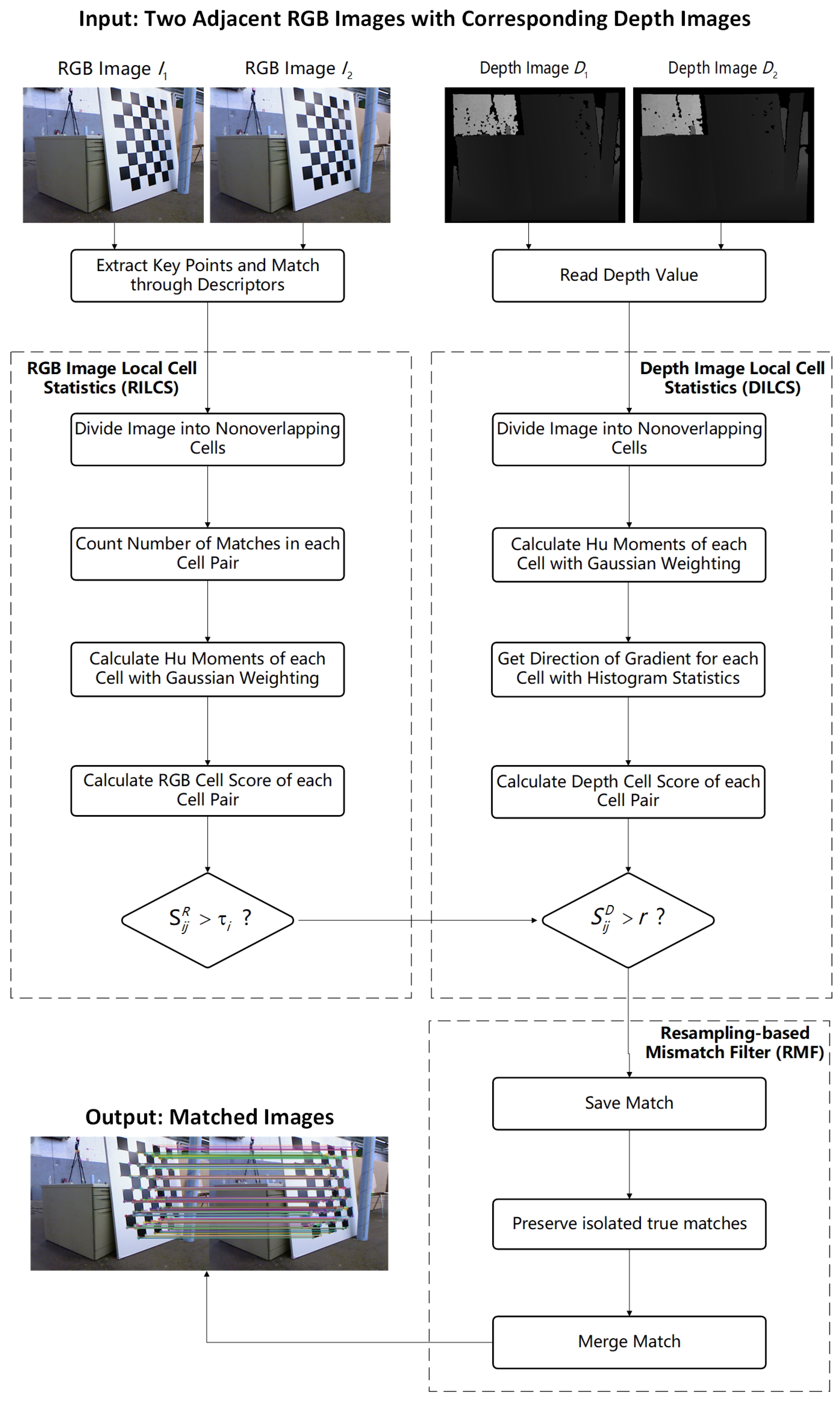
In this section, the proposed mismatch removal method LCS-SSM is presented in detail. Figure 1 demonstrates a flowchart of the proposed LCS-SSM. First, we propose an RGB image local cell statistics algorithm (RILCS) to discern potentially correct matches within a local cell region. For the input RGB images $I_1$ and $I_2$, the first step of the proposed RILCS is to extract key points. The original matched image is generated by calculating descriptors and matched key points by brute force. Then we divide $I_1$ and $I_2$ into nonoverlapping cells, which is for counting the number of matches $|M_{ij}|$ and calculating Hu moments within a local cell region conveniently. For each cell, we calculate the RGB cell score $S_{ij}^R$ that determines the cell pair of matches into the input of the proposed DILCS algorithm.

The depth image local cell statistics algorithm (DILCS) is presented to verify the reliability of the cell region. Simultaneously, for the adjacent depth images $D_1$ and $D_2$ corresponding to the RGB images $I_1$ and $I_2$, the proposed DILCS algorithm performs a similar operation to the RILCS algorithm. We divide $D_1$ and $D_2$ into the same nonoverlapping cells with $I_1$ and $I_2$, and calculate the Hu moments of each cell. Then we use the Sobel operator to detect edges for obtaining the direction of the gradient of the cell region. Then we calculate the depth cell score, which is used to ultimately determine whether a pair of matched points is correct.

Lastly, we propose a resampling-based mismatch filter algorithm (RMF) to preserve isolated true matches, which is to ensure that isolated true matches that cannot satisfy the requirement of the RILCS algorithm can be preserved. Assume that $M_t$ is a set of true matches and $M_f$ is a set of false matches that are output by the RILCS and DILCS algorithms. $M_t$ is used as an input of the RANSAC algorithm to obtain a highly reliable homography matrix that can be used to fit $M_f$ and filter out the isolated true matches.

2.1. Structural Similarity Measurement

Structural similarity is a significant metric for enhancing the robustness of image matching, and many algorithms are proposed to characterize image structural similarity. In this paper, we introduce Hu moments [39] to measure the structural similarity between images.

Hu moments of an image, as a type of image feature, exhibit desirable properties of translation, rotation, and scale invariance, which are composed of multiple normalized central moments. To obtain the Hu moments of an image, it is necessary to calculate the raw moments and central moments first. Assuming that there are M × N pixels, raw moments m and central moments $\mu$ can be calculated using the following formula:

$$m_{pq}=\sum _{x=1}^M\sum _{y=1}^{N}f(x,y)x^p{y}^q$$

(1)

$${\mu }_{pq}=\sum _{x=1}^M\sum _{y=1}^{N}f(x,y){(x-x_0)}^p{(y-y_0)}^q$$

(2)

$$\left\{\begin{array}{cc}{x}_0=& \frac{m_{10}}{m_{00}}\\ y_0=& \frac{m_{01}}{m_{00}}\end{array}\right.,$$

(3)

where $f(x,y)$ is a gray level of the pixel located at the horizontal coordinate x and the vertical coordinate y. Additionally, $x_0$, $y_0$ represents centroid coordinates of the image. We can further calculate the normalized central moments $\mu$ and Hu moments v as follows:

$${\eta }_{pq}=\frac{{\mu }_{pq}}{{\mu }_{00}^{1+\frac{p+q}{2}}}$$

(4)

$$\left\{\begin{array}{cc}{v}_1=\hfill & {\eta }_{20}+{\eta }_{02}\hfill \\ v_2=\hfill & {({\eta }_{20}-{\eta }_{02})}^2+4{\eta }_{11}^2\hfill \\ v_3=\hfill & {({\eta }_{30}-3{\eta }_{12})}^2+{(3{\eta }_{21}-{\eta }_{03})}^2\hfill \\ v_4=\hfill & {({\eta }_{30}+{\eta }_{12})}^2+{({\eta }_{21}+{\eta }_{03})}^2\hfill \\ v_5=\hfill & ({\eta }_{30}-3{\eta }_{12})({\eta }_{30}+{\eta }_{12})\hfill \\ & [{({\eta }_{30}+{\eta }_{12})}^2-3{({\eta }_{21}+{\eta }_{03})}^2]+\hfill \\ & (3{\eta }_{21}-{\eta }_{03})({\eta }_{21}+{\eta }_{03})\hfill \\ & [3{({\eta }_{30}+{\eta }_{12})}^2-{({\eta }_{21}+{\eta }_{03})}^2]\hfill \\ v_6=\hfill & ({\eta }_{20}-{\eta }_{02})[{({\eta }_{30}+{\eta }_{12})}^2-{({\eta }_{21}+{\eta }_{03})}^2]+\hfill \\ & 4{\eta }_{11}({\eta }_{30}+{\eta }_{12})({\eta }_{21}+{\eta }_{03})\hfill \\ v_7=\hfill & (3{\eta }_{21}-{\eta }_{03})({\eta }_{30}+{\eta }_{12})\hfill \\ & [{({\eta }_{30}+{\eta }_{12})}^2-3{({\eta }_{21}+{\eta }_{03})}^2]+\hfill \\ & ({\eta }_{30}-3{\eta }_{12})({\eta }_{21}+{\eta }_{03})\hfill \\ & [3{({\eta }_{30}+{\eta }_{12})}^2-{({\eta }_{21}+{\eta }_{03})}^2]\hfill \end{array}\right.$$

(5)

2.2. RGB Image Local Cell Statistics

In scenarios involving severe occlusion, deformation, or variations in illumination, local feature descriptors may lose their effective matching capability. Similarly, in images containing abundant repetitive textures, the uniqueness of descriptors might diminish, resulting in increased uncertainty in matching. Therefore, given putative matches to differentiate true and false correspondences by descriptors solely is unreliable. Meanwhile, the efficiency of the image-matching strategy based on descriptors is exhaustively needed for a real-time environment. To solve this problem, the motion consistency assumption is introduced to distinguish true and false matches, which is a simple, intuitive, and robust constraint. This basic property of motion consistency constraint assumes that objects move smoothly between image pairs, which means that pixels that are close to each other in the spatial coordinates of the image will move together. Therefore, we can assume that the likelihood that adjacent pixels belong to a single rigid object or structure results in correlated motion patterns among them. According to this, true correspondences are expected to exhibit analogous motion patterns, thereby displaying greater similarity to neighboring points within a certain region than false correspondences.

To quantify the influence caused by the analogous motion pattern of pixels, we use the number of matches within the neighborhood of the matched key points to discern true and false matches. For the input of RGB images $I_1$ and $I_2$, we set $M_{ij}$ as one of the matches across $I_1$ and $I_2$, which connects key points $f_i$ and $f_j$. Then we can define the neighborhood of $M_{ij}$ as follows:

$$N_i=\{M\ne M_{ij},d(f,f_i)<h\},$$

(6)

where d is the Euclidean distance of two points, and h is a threshold.

To discern true and false matches, we model the probability of $M_{ij}$ being correct or incorrect as follows:

$$P\sim \left\{\begin{array}{cc}B(|M|,t),& if{M}_{ij}istrue\\ B(|M|,ϵ),& if{M}_{ij}isfalse\end{array}\right.,$$

(7)

where B refers to the binomial distribution, and $|M|$ is the number of matches within $N_i$. t and $ϵ$ separately represent probabilities that M is true and false matches.

Therefore, the standardized mean difference between true and false matches can be defined as follows:

$$\begin{array}{cc}\hfill Q& =\frac{|E_t-E_f|}{\sqrt{V_t}+\sqrt{V_f}}\hfill \\ \hfill & =\frac{|M|\ast (t-ϵ)}{\sqrt{|M|\ast (t-t^2)}+\sqrt{|M|\ast (ϵ-{ϵ}^2)}},\hfill \end{array}$$

(8)

where $E_t$ and $E_f$ are expectation, and $V_t$ and $V_f$ are variations that M is true and false, respectively. It shows that we increase the number of matches $|M|$ and improve the quality of the match t; the increased separability between true and false matches leads to more reliable correct matches.

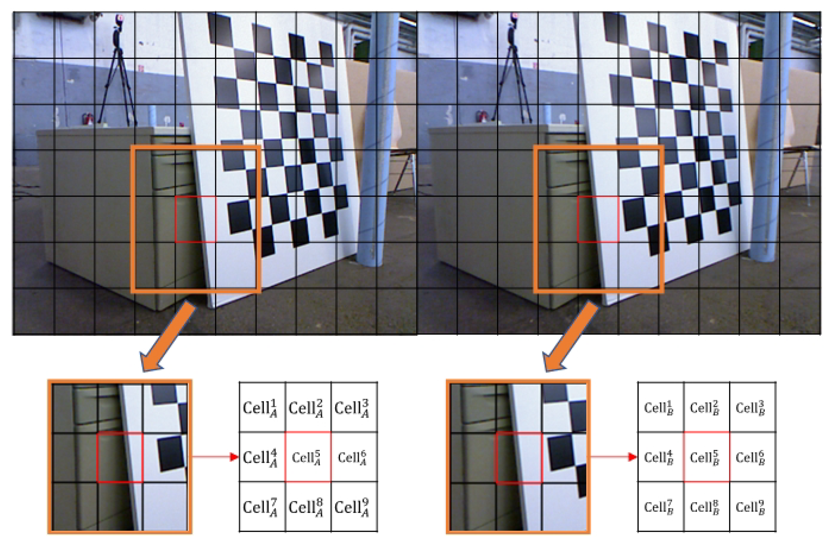
To quantify the size of the neighborhood of matched key points and enhance computational efficiency, we introduce a grid-based processing approach for images. Original image pairs are divided into nonoverlapped cells. Assuming that the resolution ratio of an image is $R_x$:$R_y$, for uniformly generating same-size cells, we determine the size of cells with the following formula:

$$\left\{\begin{array}{cc}{C}_x=& \alpha \ast R_x\\ C_y=& \alpha \ast R_y\end{array}\right.,$$

(9)

where $C_x\ast C_y$ is the resolution of each cell, and $\alpha$ is an experimental coefficient to determine the specific size of a cell.

Given specific cells in the image, such as that shown in Figure 2, with a motion consistency assumption and Equations (5), (7) and (8), we define the RGB cell score $S_{ij}^R$, which indicates that all correspondences have scores to differentiate true and false matches for an RGB image. Therefore, $S_{ij}^R$ actually refers to the score of $M_{ij}$, which indicates the correctness of matches across $Cel{l}_A^i$ and $Cel{l}_B^j$ to a certain extent, as follows:

$$S_{ij}^R=\sum _{k=1}^9|M_{i^k{j}^k}|\ast \sum _{k=1}^7\frac{|v_k^i-v_k^j|+c}{|v_k^i+v_k^j|+c},$$

(10)

where c is a constant to prevent the denominator from being zero, $M_{ij}$ is the number of matches between $Cel{l}_A^i$ and $Cel{l}_B^j$, and $v_n$ represents the n-th order Hu moment of a cell.

Let ${\tau }_i$ be the threshold of $S_{ij}^R$ to determine the cell pair of $M_{ij}$ into the input of depth image local cell statistics.

$${\tau }_i=2\sqrt{\sum _{k=1}^9|M_{i^k{j}^k}|}$$

(11)

When $S_{ij}^R>{\tau }_i$, we consider that $M_{ij}$ is potentially correct and sets the cell pair as an input of a depth image local cell statistics algorithm, which can verify the reliability of the cell region.

2.3. Depth Image Local Cell Statistics

As mentioned above, the motion consistency assumption provides a good hypothesis to limit the occurrence of a mismatch. Meanwhile, we noticed that the assumption can be invalidated at image edges, where adjacent pixels may pertain to distinct objects with independent motion patterns. To mitigate such circumstances, we use structural similarity in a depth image as a crucial constraint to differentiate between true and false correspondences.

The RGB image merely captures the chromaticity of the visual world, without providing any additional information of its inherent structure or form. Thus, it is challenging to distinguish objects with independent motion patterns in image pairs based on RGB channels. Depth images can effectively compensate for this shortcoming, which can capture the spatial information regarding the objects within a scene.

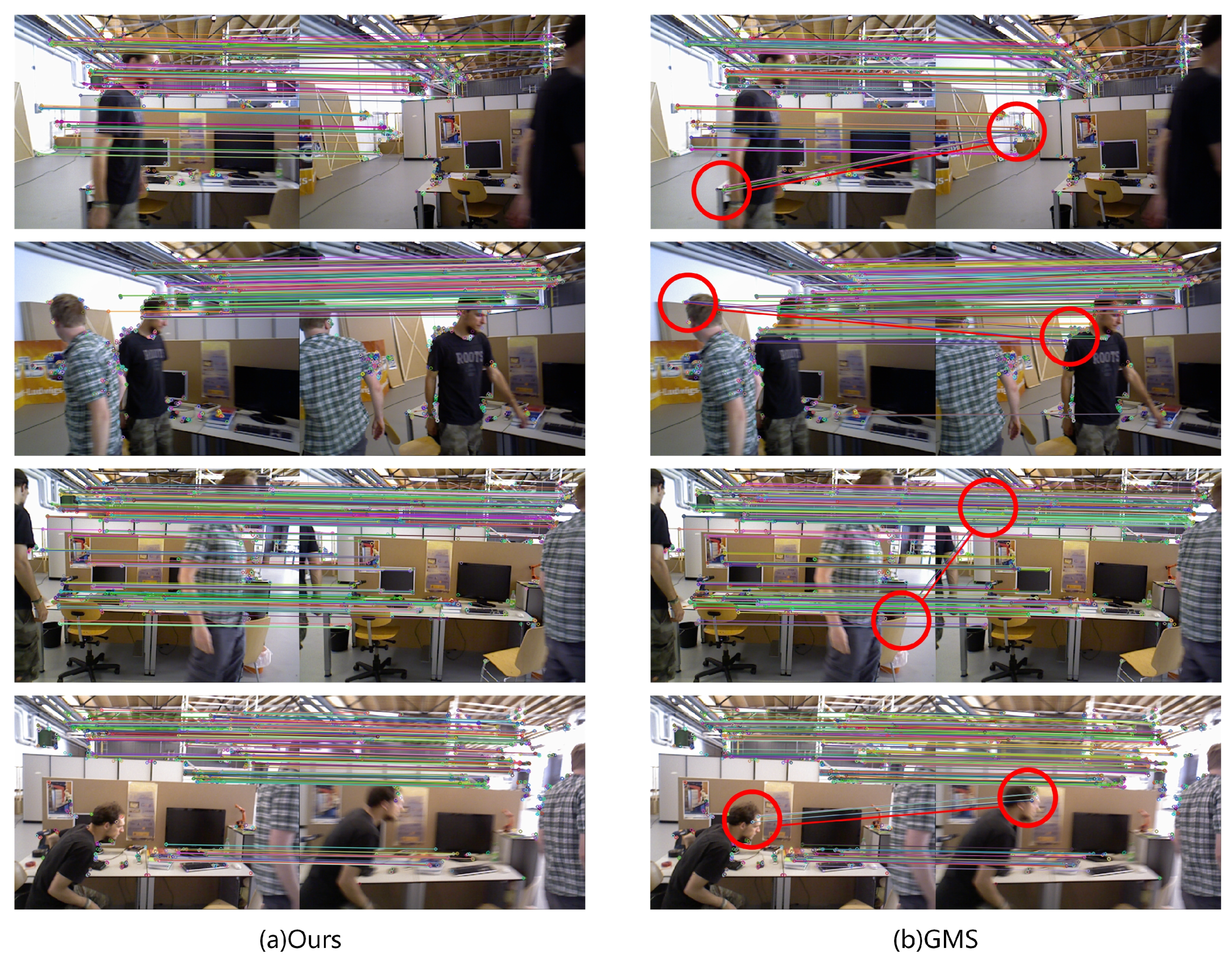
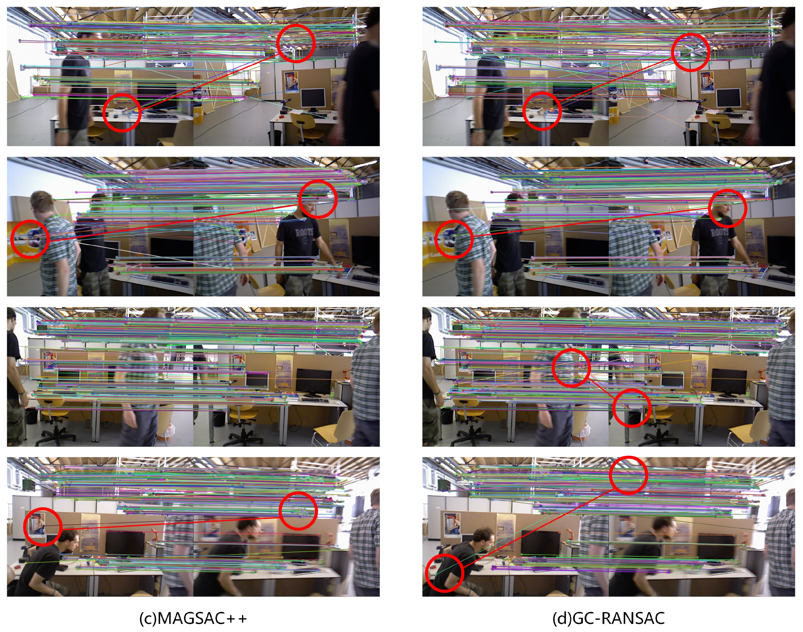
In Figure 3, there exist wrong matches caused by high-speed motion objects, which are difficult to differentiate with RGB channel images solely. Meanwhile, obvious differences between wrong matches are exposed in the same region of the corresponding depth image. There exist substantial disparities in the depth values of regions containing rapidly moving objects between two consecutive frames of depth images.

Similarly, we introduce a grid-based processing approach for depth images, which can quantify the impact of analogous motion patterns of pixels of local regions. We divide the depth image into nonoverlapping cells and utilize the structural similarity of a local region of a depth image to identify true correspondences. Let $Cell{D}_A^i$ be one of the cells in the former depth image $D_1$ and $Cel{l}_B^j$ be one of the cells in the latter depth image $D_2$. We calculate the Hu moments of each cell with Gaussian weighting; thus, we can obtain a vector of Hu moments, as follows:

$$V={[v_1,v_2,\cdots ,v_7]}^T,$$

(12)

where $v_n$ represents the n-th order a Hu moment of a cell.

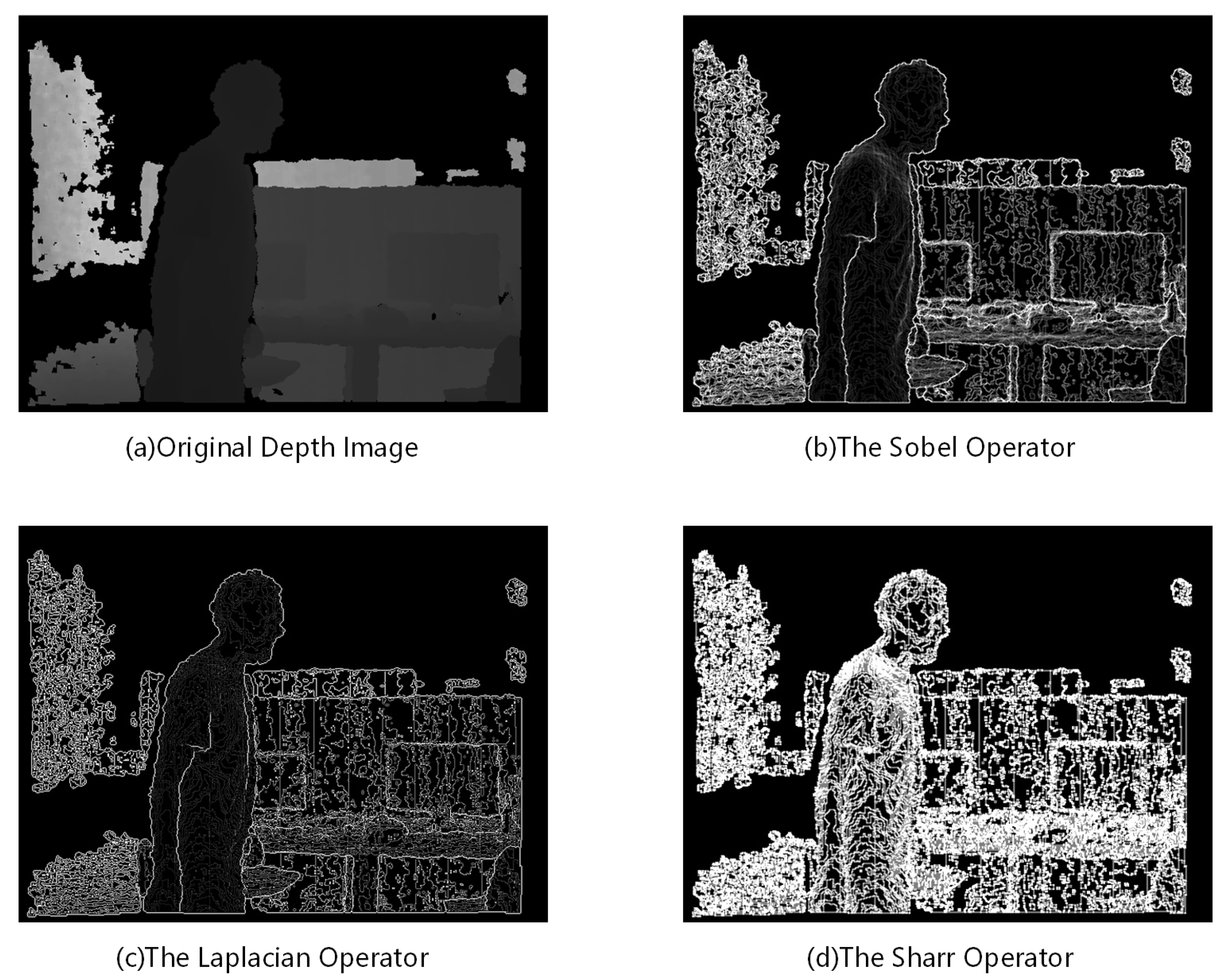
We perform edge detection using the Sobel operator to obtain the gradient of $D_1$ and $D_2$. In Figure 4, we demonstrate several edge detection algorithms for depth images. In our work, we do not place a significant emphasis on the accuracy of image edge extraction, as we need to consider the overall structure of a local region of an mage and do not require high specificity for fine textures. Therefore, using the Sobel operator for image edge detection ensures a certain degree of accuracy while maintaining high efficiency.

To obtain the main direction of the gradient of a cell that has numerous pixels, we divide the value range of a depth value into $n_{b}in$ equal bins. For each cell, we count the number of pixels $n_p$ in each bin of the value range. Let $g_M$ be the main direction of the gradient of a cell, which can be calculated by the following:

$$g_M={argmax}_k{n}_p^k$$

(13)

To enhance the robustness of the gradient direction in matching, the corresponding direction will be considered the auxiliary direction of the gradient $g_A$ for the corresponding cell if the secondary peak value exceeds 60% of the main direction peak value. Therefore, we can obtain a vector of a gradient direction as follows:

$$G={[g_M,g_A]}^T$$

(14)

With a vector of Hu moments and a gradient direction of a cell, we define the depth cell score $S_{ij}^D$ between $Cell{D}_A^i$ and $Cell{D}_B^j$ as follows:

$$S_{ij}^D=\frac{G_i·G_j+c}{|G_i|\ast |G_j|+c}\ast \frac{V_i·V_j+c}{|G_i|\ast |G_j|+c},$$

(15)

where c is a constant to prevent the denominator from being zero. Several indices of depth image are considered comprehensively, making $S_{ij}^D$ good indicators for differentiating evident motions from a background within a certain region.

Assuming that $M_{ij}$ is considered as a suspected true match, we calculate the depth cell score $S_{ij}^D$ of cells that is located in $M_{ij}$. Let r be the threshold of $S_{ij}^D$ to determine whether the matched key point is true and false matches, as follows:

$$S_{ij}^D\left\{\begin{array}{cc}>r& ,M_{ij}istrue\\ \le r& ,M_{ij}isfalse\end{array}\right.,$$

(16)

where r represents an empirical threshold used to ultimately determine whether a pair of matched points in this set is correct. Actually, a depth cell score is a combination of cosine similarities where the value range is $S_{ij}^D\in [-1,1]$; therefore, we set $r=0.8$ experimentally.

2.4. Resampling-Based Mismatch Filter

Resampling-based feature matching methods are a class of classical algorithms for mismatch removal that aim to estimate the predefined transformation model between the matched point sets, i.e., the homography matrix between two images, by repeatedly sampling from the initial matches. In this way, these methods seek to find the maximum inlier set that satisfies the estimated model as the true matches. However, these methods are limited by the reliance on the accuracy of sampling, for instance, when a large number of false matches exist in the initial matching. In such cases, not only will the estimated homography matrix have a significant error due to the presence of a large number of outliers, but also the number of sampling iterations will significantly increase, resulting in a considerable increase in the time complexity of the algorithm.

Meanwhile, RILCS algorithm perform well in the region that exists numerous matches to satisfy motion consistency assumption. However, relying solely on local cell statistics cannot identify the true matches that are isolated matches in a partial region. For there are no other matches in the neighbor to support correctness of the isolated true matches.

For preserving isolated true matches, we propose a resampling-based mismatch filter algorithm. Assume that $M_t$ is a set of true matches and $M_f$ is a set of false matches that are output by the RILCS and DILCS algorithms. For $M_t$, which is a set with a considerable number of true matches, using it as an input to the RANSAC algorithm can compensate for the dependence of resampling-based algorithms on the correctness of the initial matches. Therefore, a highly reliable homography matrix can be obtained, which can be used to fit $M_f$ and filter out the isolated true matches.

The details of the LCS-SSM algorithm will be explained in Algorithm 1.

Algorithm 1 LCS-SSM Algorithm

Require: Two adjacent RGB images $I_1$, $I_2$ and corresponding depth images $D_1$, $D_2$. Ensure: A set of true matches $S_{true}$ between $I_1$ and $I_2$.   1: Detect key points and calculate corresponding descriptors for $I_1$ and $I_2$.   2: Divide $I_1$, $I_2$, $D_1$, and $D_2$ into $C_x\times C_y$ nonoverlapping cells, respectively.   3: Locate matched key points $M_{ij}$ in $Cel{l}_A^i$ and $Cel{l}_B^j$.   4: for each matched key point $M_{ij}$ do   5:       Statistic number of matches within neighbor of $Cel{l}_A^i$ and $Cel{l}_B^j$.   6:       Calculate RGB cell score $S_{ij}^R$ and corresponding threshold ${\tau }_i$.   7:       if $S_{ij}^R>{\tau }_i$ then   8:           Save $Cel{l}_A^i$ and $Cel{l}_B^j$.   9:           Calculate depth cell score $S_{ij}^D$. 10:           if $S_{ij}^D>r$ then 11:                $S_{true}=S_{true}\cup M_{ij}$ 12:           else 13:                $S_{false}=S_{false}\cup M_{ij}$ 14:           end if 15:       end if 16: end for 17: Using $S_{true}$ as input of RANSAC algorithm to calculate homography matrix H. 18: Using H to fit $S_{false}$, preserve true matches $S_{false\to true}$ from $S_{false}$. 19: $S_{true}=S_{true}\cup S_{false\to true}$

3. Experimental Results

In this section, we conduct experiments with different key points: ORB (Oriented FAST and Rotated BRIEF) [40], SIFT [7], SURF [8], and AKAZE (Accelerated-KAZE) [41], which are well-known key point extraction algorithms. We vary the number of key points to evaluate the performance of LCS-SSM comprehensively. Meanwhile, we compare the experimental results of LCS-SSM with other three mismatch removal methods: GMS [31], MAGSAC++ [27], and GC-RANSAC [25].

We experiment on the TUM RGB-D dataset [42], where four sequences, ‘walking_xyz’, ‘walking_halfsphere’, ‘walking_static’, and ‘walking_rpy’, are employed for evaluation. We select four image pairs from those sequences respectively. The ‘walking_xyz’ and ‘walking_halfsphere’ sequences have moderate difficulty, the ‘walking_static’ sequence is a relatively easy scene for feature matching, and the ‘walking_rpy’ sequence is a challenging one. The above four sequences all have quickly moved dynamic objects within most of the scenes, which can evaluate the robustness of mismatch removal algorithms.

We utilize precision, recall, and F1-score as evaluation metrics. F1-score is a metric fusing precision and recall, which can determine the accuracy of a feature matching algorithm comprehensively. Additionally, F1-score is defined as the following formula:

$$\mathrm{F}1\text{-}\mathrm{score}={\left(\frac{Precisio{n}^{-1}+Recal{l}^{-1}}{2}\right)}^{-1}$$

(17)

As an error threshold of distance $dis{t}_{error}$ between matched key points and ground truth, we regard these matched key points that satisfy $dis{t}_{error}\le 3$ pixels as true matches.

3.1. Performance of LCS-SSM

To comprehensively evaluate the performance of LCS-SSM, we first employ four different key point extraction algorithms, ORB [40], SIFT [7], SURF [8], and AKAZE [41], to generate four key points. Then we vary the number of generated key points to examine the accuracy, which are 100, 500, 1000, 2000, and 5000, respectively.

Considering the size of a cell that can affect the accuracy of LCS-SSM, according our theory and experience, we suggest $\alpha =5,6,7,8,13$ for feature numbers $=100,500,1000,2000,5000$ in Equation (9) on the image, in which the resolution is $640\times 480$.

Figure 5 shows the results of the varying number of key points. The numbers 100, 500, 1000, 2000, and 5000 are the number of key points. It is noticed that when the number of key points is set in a certain range, e.g., 500 to 2000, the precision, recall, and F1-score are all maintained at a high level.

When we decrease the number of key points to 100, LCS-SSM can be validated by the lack of feature number because the generated matched key points are dispersed and insufficient to reach the requirement of the RILCS algorithm. The SIFT [7] and SURF [8] algorithms extract abundant feature information, making them typically suitable for cases requiring high-quality feature points. However, when fewer key points are needed, they may not provide sufficient key points. Particularly with the SIFT [7] algorithm, even when we increase the number of key points to 500 on the ‘walking_rpy’ sequence, it still cannot provide enough key points to meet the requirements of the RILCS algorithm. The ORB [40] algorithm has high computational efficiency and can still provide a large number of key points even in the presence of a blur and low-image texture. Therefore, when we reduce the number of key points to 100, it can typically provide a sufficient quantity of key points in most cases, with a limited impact on accuracy.

When we increased the number of key points to 5000, we found that some key point extraction algorithms cannot provide sufficient key points and may generate more wrong matches than true matches. Especially with the SURF [8] and AKAZE [41] algorithms, when we increase the number of key points to 2000 or even 5000, the quality of the key points they provide deteriorates significantly. As a result, the accuracy of matching is severely decreased by insufficient matched key points and numerous wrong matches.

We also experiment to evaluate the runtime of LCS-SSM with a varying number of key points on four sequences. Figure 6 shows the results that LCS-SSM takes about “0.05 s” in processing a pair of RGBD images in a single CPU thread. When more key points are needed, compared with other algorithms, the ORB [40] algorithm typically provides a larger number of key points. As a result, more time is spent by the LCS-SSM algorithm. Conversely, the SIFT [7] algorithm extracts fewer key points, leading to reduced computational complexity. The runtime of LCS-SSM has increased as we increase the number of key points. Most of the compensation of the runtime is in calculating the RGB cell score and depth cell score so that the runtime can be further compressed by multi-threading programming.

3.2. Comparison with Other Existing Methods

To demonstrate the superiority of LCS-SSM, we examine other mismatch removal methods, GMS [31], MAGSAC++ [27], and GC-RANSAC [25], under the same circumstances to compare their performances with LCS-SSM. To better evaluate the performance differences among these methods, we set the number of key points to 1000. Then we use four different key point extraction algorithms, ORB [40], SIFT [7], SURF [8], and AKAZE [41], to generate four key points.

Figure 7 shows the comparison the results of these methods, which show that LCS-SSM has higher performance compared with the other methods. As can be seen, it is evident that, when dealing with scenarios involving low-speed moving objects, LCS-SSM outperforms other algorithms and achieves the optimal results in the task of mismatch removal. For instance, when using the SIFT [7] algorithm for feature extraction, LCS-SSM exhibits superior accuracy compared with the sub-optimal performance of GMS [31]. The recall rate of LCS-SSM is as optimal as that of GC-RANSAC [25], and its F1-score also ranks as the best. Even in scenarios involving medium-speed moving objects, the LCS-SSM algorithm continues to achieve the optimal results in terms of precision, recall, and F1-score across multiple experiments. When high-speed moving objects appear in the images to be matched, the performances of all four algorithms decline. However, when using ORB [40], SURF [8], and AKAZE [41] feature points, the LCS-SSM algorithm still exhibits the best precision and F1-score compared with the other algorithms. It is evident that LCS-SSM significantly outperforms other algorithms in terms of precision, although its recall rate is slightly lower than those of others. Therefore, LCS-SSM maintains the optimal results in terms of F1-score.

Compared with other methods, LCS-SSM demonstrates a clear advantage in both accuracy and F1-score, but the superiority of LCS-SSM in recall is not evident. The MAGSAC++ [27] and GC-RANSAC [25] algorithms achieve a high recall rate, but noticeable mismatches still exist in the images. When mismatches are caused by moving objects, the GMS [31] algorithm fails to effectively filter out such mismatches. Moreover, the mismatch removal results often show a phenomenon of highly concentrated dispersion of feature points, making it unable to effectively discern isolated feature matches.

We consider that ‘walking_rpy’ is a sequence that exists quickly moving objects, and the camera motion is extremely intense. SIFT [7] itself is a key point extraction algorithm that possesses high requirements when generating key points, which means that it cannot provide sufficient correct matched key points under challenging scenarios. Thus, the performance of mismatch removal methods that rely on the geometric constraint, e.g., motion consistency consumption, like LCS-SSM and GMS [31], is worse than those of MAGSAC++ [27] and GC-RANSAC [25].

In contrast, these four methods all perform well in the ‘walking_static’ sequence, which has a relatively easy scene. Due to the slow speed of moving objects in the images to be matched, the interference with the matching results is limited. Additionally, the camera movement speed is also slow, with hardly any occurrence of image blur, and the ORB [40], SIFT [7], SURF [8], and AKAZE [41] algorithms can all provide an adequate number of feature points. Nevertheless, the LCS-SSM algorithm still outperforms other algorithms in terms of accuracy.

In Figure 8, we demonstrate the visual image results of these methods with ORB [40] on four sequences. The correct matches are connected by a line of the same color, and we have marked some regions with obvious mismatches. It can be seen that MAGSAC++ [27] and GC-RANSAC [25] both have evidently wrong matches. Compared with the above two methods, GMS [31] has fewer obviously wrong matches. However, LCS-SSM is undoubtedly the most outstanding algorithm in terms of visual performance, as it has almost no obvious wrong matches and retains a sufficiently large number of correct matches.

4. Discussion

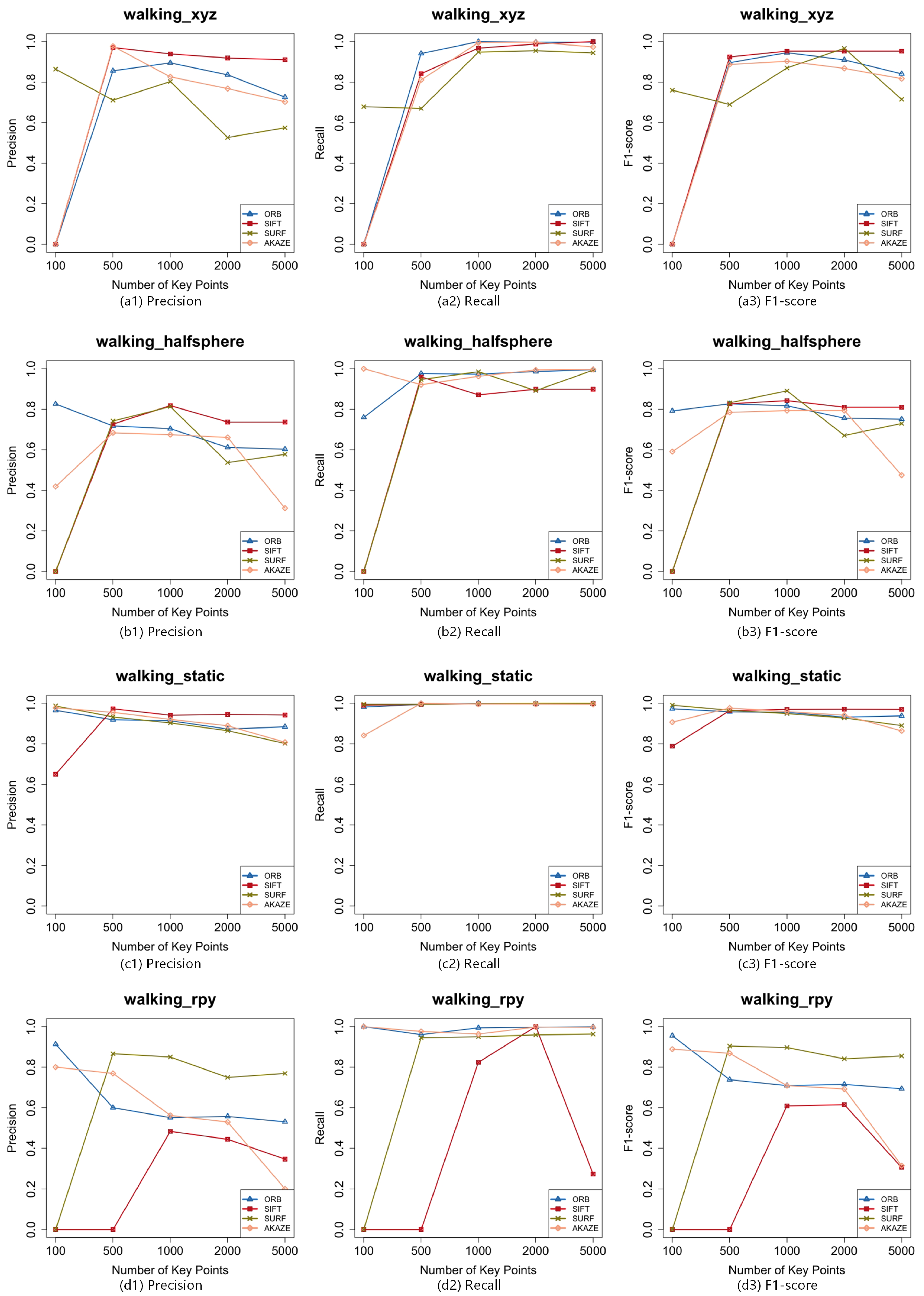
Traditional feature matching methods are unreliable because they solely rely on feature detectors and descriptors to distinguish true and false correspondences. To solve this problem, we introduce a simple, intuitive, and robust constraint and motion consistency assumption, which assumes that pixels that are close to each other in the spatial coordinates of the image will move together. However, this assumption does not invariably hold true, which can be invalidated at image edges, where adjacent pixels may pertain to distinct objects with independent motion patterns. We select four sequences from the TUM RGB-D dataset, which all have quickly moving dynamic objects within most of the scenes that can invalidate the motion consistency assumption. The performance of methods like GMS, which is solely based on the motion consistency assumption, is demonstrated in Figure 3. To inhibit the impact of the above scenarios, we introduce another crucial element, the structural similarity of an image, which is a significant metric that can reflect the similarity in structure between two images, to further eliminate more wrong matches that satisfy the motion consistency assumption. In addition, we utilize a resampling method to preserve isolated true matches that dissatisfy the RILCS. By integrating the aforementioned theories and methods, we propose the LCS-SSM algorithm.

However, it has to be mentioned that LCS-SSM requires a sufficient number of matched key points to obtain as many as possible true matches. The accuracy of LCS-SSM is decreased by insufficient matched key points. Especially when facing a scene with low texture and structure and using the key point extraction algorithm that cannot provide adequate true matched key points in the challenging scenario, LCS-SSM may be invalidated. Therefore, how to improve the performance of the mismatch removal method in cases with low texture and having fewer key points is the next work of our team.

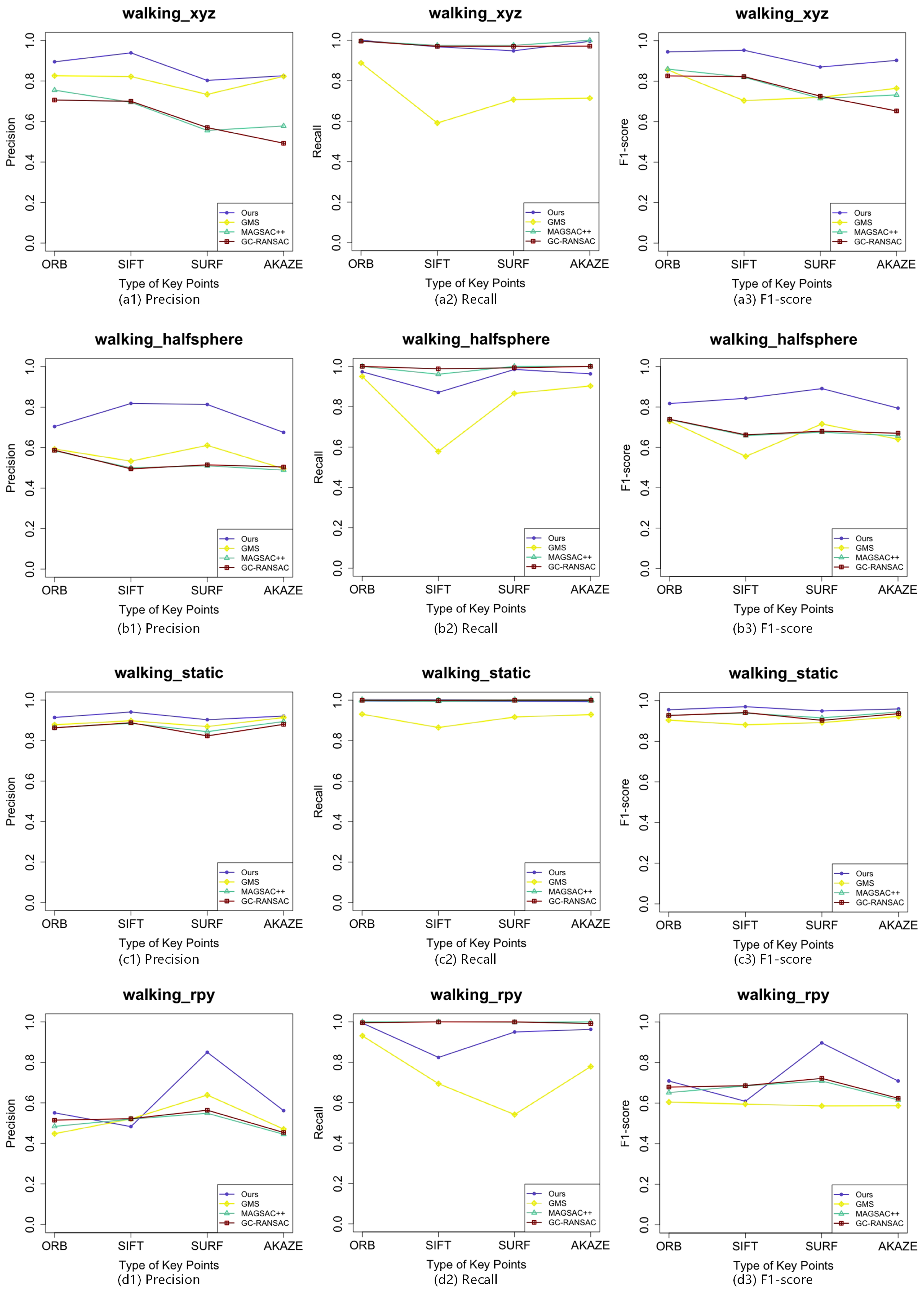
According to our experimental results, LCS-SSM performs well in using various types of key points and sequences with different difficulties, which is the most outstanding algorithm compared with the state-of-the-art methods in the area of mismatch removal. More specifically, the precision performance of LCS-SSM using SURF on the four sequences has improved by 19.38% on average, which is the highest compared with the values of 9.1% of ORB, 13.91% of SIFT, and 12.6% of AKAZE. However, it can be seen from Figure 7 that the recall performance of LCS-SSM is slightly lower than those of others. The F1-score performance of LCS-SSM has improved by 7% using ORB, 9.83% by using SIFT, 15.55% by using SURF, and 11.23% by using AKAZE. In terms of the runtime of LCS-SSM, although the execution times are related to the number of key points, it maintains high efficiency even when processing 5000 key points. It costs about 50 milliseconds to process a pair of RGBD images in a single CPU thread.

5. Conclusions

In this paper, we propose a robust mismatch removal method, the LCS-SSM algorithm. It leverages the motion consistency assumption and structural similarity of an RGB image and a depth image to obtain true correspondences. Moreover, we utilize the RANSAC algorithm to save isolated true matches that are filtered by the RILCS. We conduct a series of experiments comprehensively to verify the performance of LCS-SSM, which demonstrates high robustness and accuracy in the environment that exists in dynamic objects. We will focus on the above problem and improve the performance of the proposed mismatch removal method in our future work.

References

1. Ma, J.; Jiang, X.; Fan, A.; Jiang, J.; Yan, J. Image matching from handcrafted to deep features: A survey. Int. J. Comput. Vis. 2021, 129, 23–79. [Google Scholar] [CrossRef]
2. Campos, C.; Elvira, R.; Rodríguez, J.J.G.; Montiel, J.M.; Tardós, J.D. Orb-slam3: An accurate open-source library for visual, visual–inertial, and multimap slam. IEEE Trans. Robot. 2021, 37, 1874–1890. [Google Scholar] [CrossRef]
3. Qin, T.; Li, P.; Shen, S. Vins-mono: A robust and versatile monocular visual-inertial state estimator. IEEE Trans. Robot. 2018, 34, 1004–1020. [Google Scholar] [CrossRef]
4. Schonberger, J.L.; Frahm, J.M. Structure-from-motion revisited. In Proceedings of the IEEE Conference on Computer Vision and Pattern Recognition, Las Vegas, NV, USA, 27–30 June 2016; pp. 4104–4113. [Google Scholar]
5. Hu, T.; Sun, X.; Su, Y.; Guan, H.; Sun, Q.; Kelly, M.; Guo, Q. Development and performance evaluation of a very low-cost UAV-LiDAR system for forestry applications. Remote Sens. 2020, 13, 77. [Google Scholar] [CrossRef]
6. Mescheder, L.; Oechsle, M.; Niemeyer, M.; Nowozin, S.; Geiger, A. Occupancy networks: Learning 3d reconstruction in function space. In Proceedings of the IEEE/CVF Conference on Computer Vision and Pattern Recognition, Long Beach, CA, USA, 15–20 June 2019; pp. 4460–4470. [Google Scholar]
7. Lowe, D.G. Distinctive image features from scale-invariant keypoints. Int. J. Comput. Vis. 2004, 60, 91–110. [Google Scholar] [CrossRef]
8. Bay, H.; Tuytelaars, T.; Van Gool, L. Surf: Speeded up robust features. In Proceedings of the Computer Vision–ECCV 2006: 9th European Conference on Computer Vision, Graz, Austria, 7–13 May 2006; Proceedings, Part I 9. Springer: Berlin/Heidelberg, Germany, 2006; pp. 404–417. [Google Scholar]
9. Ke, Y.; Sukthankar, R. PCA-SIFT: A more distinctive representation for local image descriptors. In Proceedings of the 2004 IEEE Computer Society Conference on Computer Vision and Pattern Recognition, 2004. CVPR 2004, Washington, DC, USA, 27 June–2 July 2004; Volume 2, p. II. [Google Scholar]
10. Calonder, M.; Lepetit, V.; Strecha, C.; Fua, P. Brief: Binary robust independent elementary features. In Proceedings of the Computer Vision–ECCV 2010: 11th European Conference on Computer Vision, Heraklion, Crete, Greece, 5–11 September 2010; Proceedings, Part IV 11. Springer: Berlin/Heidelberg, Germany, 2010; pp. 778–792. [Google Scholar]
11. Leutenegger, S.; Chli, M.; Siegwart, R.Y. BRISK: Binary robust invariant scalable keypoints. In Proceedings of the 2011 International Conference on Computer Vision, Barcelona, Spain, 6–13 November 2011; pp. 2548–2555. [Google Scholar]
12. Alahi, A.; Ortiz, R.; Vandergheynst, P. Freak: Fast retina keypoint. In Proceedings of the 2012 IEEE Conference on Computer Vision and Pattern Recognition, Providence, RI, USA, 16–21 June 2012; pp. 510–517. [Google Scholar]
13. Heule, M.J.; Kullmann, O. The science of brute force. Commun. ACM 2017, 60, 70–79. [Google Scholar] [CrossRef]
14. Muja, M.; Lowe, D.G. Fast approximate nearest neighbors with automatic algorithm configuration. VISAPP (1) 2009, 2, 2. [Google Scholar]
15. Verdie, Y.; Yi, K.; Fua, P.; Lepetit, V. Tilde: A temporally invariant learned detector. In Proceedings of the IEEE Conference on Computer Vision and Pattern Recognition, Boston, MA, USA, 7–12 June 2015; pp. 5279–5288. [Google Scholar]
16. Yi, K.M.; Trulls, E.; Lepetit, V.; Fua, P. Lift: Learned invariant feature transform. In Proceedings of the Computer Vision–ECCV 2016: 14th European Conference, Amsterdam, The Netherlands, 11–14 October 2016; Proceedings, Part VI 14. Springer: Berlin/Heidelberg, Germany, 2016; pp. 467–483. [Google Scholar]
17. DeTone, D.; Malisiewicz, T.; Rabinovich, A. Superpoint: Self-supervised interest point detection and description. In Proceedings of the IEEE Conference on Computer Vision and Pattern Recognition Workshops, Salt Lake City, UT, USA, 18–22 June 2018; pp. 224–236. [Google Scholar]
18. Sarlin, P.E.; DeTone, D.; Malisiewicz, T.; Rabinovich, A. Superglue: Learning feature matching with graph neural networks. In Proceedings of the IEEE/CVF Conference on Computer Vision and Pattern Recognition, Seattle, WA, USA, 13–19 June 2020; pp. 4938–4947. [Google Scholar]
19. Wang, P.; Wang, L.; Leung, H.; Zhang, G. Super-resolution mapping based on spatial–spectral correlation for spectral imagery. IEEE Trans. Geosci. Remote Sens. 2020, 59, 2256–2268. [Google Scholar] [CrossRef]
20. Li, H.; Wu, X.J.; Durrani, T. NestFuse: An infrared and visible image fusion architecture based on nest connection and spatial/channel attention models. IEEE Trans. Instrum. Meas. 2020, 69, 9645–9656. [Google Scholar] [CrossRef]
21. Fischler, M.A.; Bolles, R.C. Random sample consensus: A paradigm for model fitting with applications to image analysis and automated cartography. Commun. ACM 1981, 24, 381–395. [Google Scholar] [CrossRef]
22. Torr, P.H.; Zisserman, A. MLESAC: A new robust estimator with application to estimating image geometry. Comput. Vis. Image Underst. 2000, 78, 138–156. [Google Scholar] [CrossRef]
23. Chum, O.; Matas, J.; Kittler, J. Locally optimized RANSAC. In Proceedings of the Pattern Recognition: 25th DAGM Symposium, Magdeburg, Germany, 10–12 September 2003; Proceedings 25. Springer: Berlin/Heidelberg, Germany, 2003; pp. 236–243. [Google Scholar]
24. Chum, O.; Matas, J. Matching with PROSAC-progressive sample consensus. In Proceedings of the 2005 IEEE Computer Society Conference on Computer Vision and Pattern Recognition (CVPR’05), San Diego, CA, USA, 20–25 June 2005; Volume 1, pp. 220–226. [Google Scholar]
25. Barath, D.; Matas, J. Graph-cut RANSAC. In Proceedings of the IEEE Conference on Computer Vision and Pattern Recognition, Salt Lake City, UT, USA, 18–23 June 2018; pp. 6733–6741. [Google Scholar]
26. Barath, D.; Matas, J.; Noskova, J. MAGSAC: Marginalizing sample consensus. In Proceedings of the IEEE/CVF Conference on Computer Vision and Pattern Recognition, Long Beach, CA, USA, 15–20 June 2019; pp. 10197–10205. [Google Scholar]
27. Barath, D.; Noskova, J.; Ivashechkin, M.; Matas, J. MAGSAC++, a fast, reliable and accurate robust estimator. In Proceedings of the IEEE/CVF Conference on Computer Vision and Pattern Recognition, Seattle, WA, USA, 13–19 June 2020; pp. 1304–1312. [Google Scholar]
28. He, Z.; Shen, C.; Wang, Q.; Zhao, X.; Jiang, H. Mismatching removal for feature-point matching based on triangular topology probability sampling consensus. Remote Sens. 2022, 14, 706. [Google Scholar] [CrossRef]
29. Raguram, R.; Chum, O.; Pollefeys, M.; Matas, J.; Frahm, J.M. USAC: A universal framework for random sample consensus. IEEE Trans. Pattern Anal. Mach. Intell. 2012, 35, 2022–2038. [Google Scholar] [CrossRef]
30. Ma, J.; Zhao, J.; Tian, J.; Yuille, A.L.; Tu, Z. Robust point matching via vector field consensus. IEEE Trans. Image Process. 2014, 23, 1706–1721. [Google Scholar] [CrossRef]
31. Bian, J.; Lin, W.; Matsushita, Y.; Yeung, S.; Nguyen, T.; Cheng, M. GMS: Grid-Based Motion Statistics for Fast, Ultra-robust Feature Correspondence. Int. J. Comput. Vis. 2020, 128, 1580–1593. [Google Scholar] [CrossRef]
32. Ma, J.; Zhao, J.; Jiang, J.; Zhou, H.; Guo, X. Locality preserving matching. Int. J. Comput. Vis. 2019, 127, 512–531. [Google Scholar] [CrossRef]
33. Ma, J.; Fan, A.; Jiang, X.; Xiao, G. Feature matching via motion-consistency driven probabilistic graphical model. Int. J. Comput. Vis. 2022, 130, 2249–2264. [Google Scholar] [CrossRef]
34. Karpushin, M.; Valenzise, G.; Dufaux, F. Keypoint detection in rgbd images based on an anisotropic scale space. IEEE Trans. Multimed. 2016, 18, 1762–1771. [Google Scholar] [CrossRef]
35. Karpushin, M.; Valenzise, G.; Dufaux, F. TRISK: A local features extraction framework for texture-plus-depth content matching. Image Vis. Comput. 2018, 71, 1–16. [Google Scholar] [CrossRef]
36. Cong, R.; Lei, J.; Fu, H.; Huang, Q.; Cao, X.; Hou, C. Co-saliency detection for RGBD images based on multi-constraint feature matching and cross label propagation. IEEE Trans. Image Process. 2017, 27, 568–579. [Google Scholar] [CrossRef]
37. Bao, J.; Yuan, X.; Huang, G.; Lam, C.T. Point Cloud Plane Segmentation-Based Robust Image Matching for Camera Pose Estimation. Remote Sens. 2023, 15, 497. [Google Scholar] [CrossRef]
38. Bao, J.; Yuan, X.; Lam, C.T. Robust Image Matching for Camera Pose Estimation Using Oriented Fast and Rotated Brief. In Proceedings of the 2022 5th International Conference on Algorithms, Computing and Artificial Intelligence, Sanya, China, 23–25 December 2022; pp. 1–5. [Google Scholar]
39. Liu, Y.; Yin, Y.; Zhang, S. Hand gesture recognition based on HU moments in interaction of virtual reality. In Proceedings of the 2012 4th International Conference on Intelligent Human-Machine Systems and Cybernetics, Nanchang, China, 26–27 August 2012; Volume 1, pp. 145–148. [Google Scholar]
40. Rublee, E.; Rabaud, V.; Konolige, K.; Bradski, G. ORB: An efficient alternative to SIFT or SURF. In Proceedings of the 2011 International Conference on Computer Vision, Barcelona, Spain, 6–13 November 2011; pp. 2564–2571. [Google Scholar]
41. Alcantarilla, P.F.; Solutions, T. Fast explicit diffusion for accelerated features in nonlinear scale spaces. IEEE Trans. Patt. Anal. Mach. Intell. 2011, 34, 1281–1298. [Google Scholar]
42. Sturm, J.; Engelhard, N.; Endres, F.; Burgard, W.; Cremers, D. A benchmark for the evaluation of RGB-D SLAM systems. In Proceedings of the 2012 IEEE/RSJ International Conference on Intelligent Robots and Systems, Vilamoura-Algarve, Portugal, 7–12 October 2012; pp. 573–580. [Google Scholar]
Figure 1. Flowchart of the proposed LCS-SSM. For the input of two adjacent RGB and depth images, the RILCS divides I 1 and I 2 into nonoverlapping cells for calculating the RGB cell score of each cell region to determine the cell pair of matches into the input of the DILCS. Meanwhile, the DILCS divides D 1 and D 2 into the same nonoverlapping cells with I 1 and I 2 and calculate the Hu moments of each cell. Then the DILCS performs edge detection on D 1 and D 2 to obtain the main and auxiliary direction of the gradient of the cell region. Then the DILCS calculates the depth cell score to verify the reliability of the cell region. Lastly, the RMF utilizes the output of the RILCS and the DILCS to further filter isolated true matches that cannot satisfy the requirement of the RILCS.
Remotesensing 16 01873 g001
Figure 2. A local region for a cell pair to calculate a score. Assuming that a pair of matches are located in C e l l A 5 and C e l l B 5 , we use other matches around the matches that we considered to calculate the RGB cell score S i j R .
Remotesensing 16 01873 g002
Figure 3. Wrong matches caused by a high motion object. The regions with obvious mismatches in the RGBD images have been marked with red circles.
Remotesensing 16 01873 g003
Figure 4. Several edge detection algorithms of a depth image.
Remotesensing 16 01873 g004
Figure 5. Experimental results of four key points with a varying number of key points on four different sequences: (a1a3) the precision, recall, and F1-score of LCS-SSM on ‘walking_xyz’; (b1b3) the precision, recall, and F1-score of LCS-SSM on ‘walking_halfsphere’; (c1c3) the precision, recall, and F1-score of LCS-SSM on ‘walking_static’; (d1d3) the precision, recall, and F1-score of LCS-SSM on ‘walking_rpy’.
Remotesensing 16 01873 g005
Figure 6. The runtime of LCS-SSM with a varying number of key points on four different sequences: (a) the runtime of LCS-SSM on ‘walking_xyz’, (b) the runtime of LCS-SSM on ‘walking_halfsphere’, (c) the runtime of LCS-SSM on ‘walking_static’, and (d) the runtime of LCS-SSM on ‘walking_rpy’.
Remotesensing 16 01873 g006
Figure 7. Comparison results of LCS-SSM, GMS, MAGSAC++, and GC-RANSAC: (a1a3) the precision, recall, and F1-score on ‘walking_xyz’; (b1b3) the precision, recall, and F1-score on ‘walking_halfsphere’; (c1c3) the precision, recall, and F1-score on ‘walking_static’; and (d1d3) the precision, recall, and F1-score on ‘walking_rpy’.
Remotesensing 16 01873 g007
Figure 8. Visual image results of LCS-SSM, GMS, MAGSAC++, and GC-RANSAC with ORB on ‘walking_xyz’, ‘walking_halfsphere’, ‘walking_static’, and ‘walking_rpy’. The regions with obvious mismatches in the image have been marked with red circles and lines. (a) Ours, (b) GMS, (c) MAGSAC++, and (d) GC-RANSAC.
Remotesensing 16 01873 g008aRemotesensing 16 01873 g008b
Disclaimer/Publisher’s Note: The statements, opinions and data contained in all publications are solely those of the individual author(s) and contributor(s) and not of MDPI and/or the editor(s). MDPI and/or the editor(s) disclaim responsibility for any injury to people or property resulting from any ideas, methods, instructions or products referred to in the content.