Examining the Impacts of Pre-Fire Forest Conditions on Burn Severity Using Multiple Remote Sensing Platforms

Abstract

Pre-fire environmental conditions play a critical role in wildfire severity. This study investigated the impact of pre-fire forest conditions on burn severity as a result of the 2020 Bighorn Fire in the Santa Catalina Mountains in Arizona. Using a stepwise regression model and remotely sensed data from Landsat 8 and LiDAR, we analyzed the effects of structural and functional vegetation traits and environmental factors on burn severity. This analysis revealed that the difference normalized burn ratio (dNBR) was a more reliable indicator of burn severity compared to the relative dNBR (RdNBR). Stepwise regression identified pre-fire normalized difference vegetation index (NDVI), canopy cover, and tree density as significant variables across all land cover types that explained burn severity, suggesting that denser areas with higher vegetation greenness experienced more severe burns. Interestingly, residuals between the actual and estimated dNBR were lower in herbaceous zones compared to denser forested areas at similar elevations, suggesting potentially more predictable burn severity in open areas. Spatial analysis using Geary’s C statistics further revealed a strong negative autocorrelation: areas with high burn severity tended to be clustered, with lower severity areas interspersed. Overall, this study demonstrates the potential of readily available remote sensing data to predict potential burn severity values before a fire event, providing valuable information for forest managers to develop strategies for mitigating future wildfire damage.

1. Introduction

Wildfires are an essential forest process, but contemporary fires pose significant challenges to forests, resulting in substantial alterations to their structure and function [1,2,3]. Fires can contribute to soil erosion, reduced capacity for carbon storage, and changes in ecosystem processes and forest health [4,5]. The Southwestern U.S. has witnessed a substantial increase in wildfire occurrence, generally attributed to extreme droughts and the accumulation of uncharacteristically abundant fuels [6]. Additionally, the legacy of past fires (or their suppression) can impact the severity of subsequent fires by influencing vegetation types and the time available for fuels to regenerate [7].

Burn severity, defined as the extent of environmental change caused by fire [8], carries multiple ecological implications. Severity is the direct consequence of fire behavior, exhibits a direct correlation with carbon emissions [9], and has significant impacts on vegetation and soils as well as the potential to profoundly influence the trajectory of ecosystem responses [10]. Given the extensive damage caused by uncharacteristically high-severity contemporary fires, accurately revealing the relationship between pre-fire conditions and burn severity could provide a valuable method to anticipate wildfire impacts [11] that is crucial for prioritizing fuel management efforts [12], refining the quantification of fire-carbon dynamics [13], and forecasting ecosystem impacts [10]. The magnitude of burn severity is co-influenced by environmental factors that regulate fire behavior including wind, relative humidity, fuel loads, forest density, live and dead fuel moisture content, and terrain characteristics, making it challenging to attribute specific variables to variations in burn severity [14].

Prior studies have demonstrated that burn severity hinges strongly on the dominant vegetation cover types and forest structure because these factors are central to fire behavior [15,16]. Research focusing on the spatial variability of burn severity commonly represents vegetation and fuels primarily through digital maps of vegetation types, land cover, and terrain factors [17] including slope, aspect, and the eastness and northness of the slope. In areas with rugged terrain, these maps are sometimes supplemented with a limited set of stand structural variables measured in the field [12]. However, this is frequently accomplished using plot data, which only sample a small fraction of the landscape. The increasing availability of light detection and ranging (LiDAR) data presents an opportunity to obtain additional insights into the horizontal and vertical structure of pre-fire vegetation, which can significantly enhance our understanding of how vegetation and fuels contribute to fire severity [18].

The influence of topography on fire severity is intricate and variable, often yielding conflicting findings. These intricacies arise from the complex interactions between topography, fuels, and fire behavior [19,20]. Some research has indicated that extreme fire weather conditions can override or alter the relationships between topography and fire severity [21]. Assessing the robustness of these findings can be challenging, as only a limited number of studies have incorporated fire progression data to evaluate the alignment between topographical features and the advancing fire front [19].

To establish the relationship between pre-fire forest attributes and burn severity, it is essential to explore their connections to the actual expressed severity. Finer spatial resolution forest structure datasets, obtained through CubeSats, UAVs, or LiDAR, are becoming increasingly available as well as the traditional coarser multispectral remotely sensed datasets [22]. Coupled with machine learning classification methods and various resolution datasets, forest structural classification can help explain the variations in burn severity by focusing on pre-fire structural diversity [23].

The primary aim of this research was to investigate how pre-fire forest conditions impacted the burn severity in a study landscape and to identify which pre-fire variables accounted for variations in fire severity across the landscape. To achieve this objective, we identified a suite of pre-fire structural and functional traits using aerial LiDAR and Landsat 8 data. These traits were used as predictor variables to model the burn severity of the 2020 Bighorn Fire in the Santa Catalina Mountains (SCMs), one of the Sky Island mountain ranges in southern Arizona, USA. Understanding the relationship between these variables and severity, by modifying fire behavior, is crucial for managing and mitigating the impact of wildfires on our forests.

2. Study Area and Methods

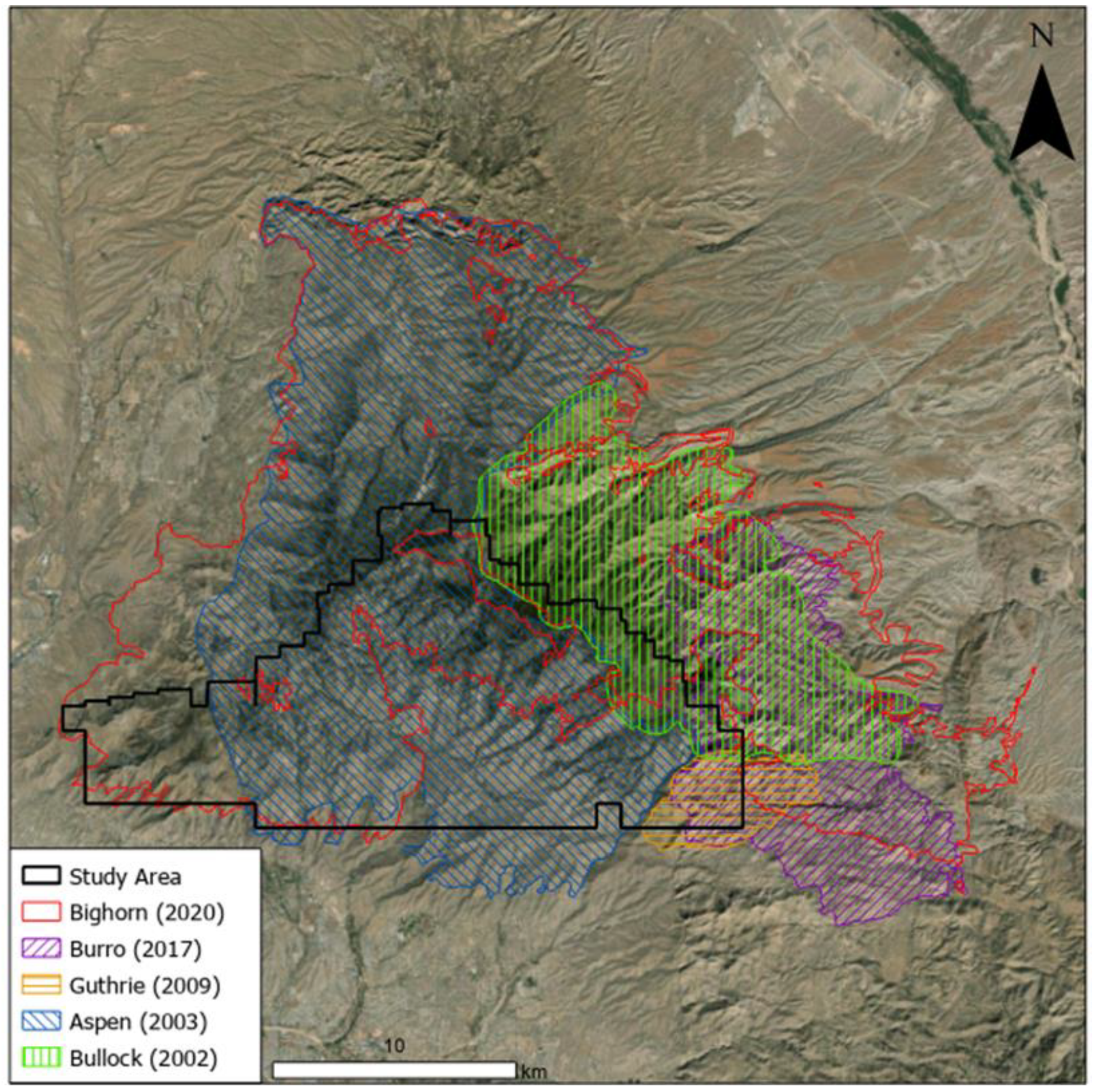
2.1. Study Area and Fire Regime

For centuries up until the late-19th century, the southwest region of the United States experienced a fire regime very different from the present day. At that time, fires were frequent, occurring every 5–20 years, and typically of low intensity. These fires were predominantly ignited by lightning strikes [24] or by Native American practices [25]. Because fires were frequent, often burning for weeks under moderate conditions, fuel accumulation was limited, and consequently, the fire severity was generally moderate [26]. However, toward the end of the 19th century, changes in land management such as livestock grazing and fire suppression policies brought about a significant transformation in the fire regime [27,28]. Urban expansion and agricultural activities further altered landscapes, disrupting natural fire cycles and fuel distribution [29]. During the mid-20th century, aggressive fire suppression efforts became commonplace, with the aim of extinguishing all wildfires, regardless of their natural role or size [30]. The combined impact of fire suppression, overgrazing, and changes in land use resulted in a reduced area being burned, leading to the accumulation of fuel and the uniformity of landscapes. This led to a decrease in vegetation diversity and an increase in the prevalence of fire-prone species like Bromus tectorum (cheatgrass) and other non-native grasses, contributing to more widespread and devastating fires [31].

In 2020, the southwest region of the United States, comprising Arizona and New Mexico, experienced a substantial wildfire season that led to the burning of 432,355 ha and the average area burned annually in the two states over the preceding ten-year period [32]. Wildfires in Arizona covered a significantly larger area (376,164 ha) in 2020 compared to its ten-year annual average of 123,681 ha. New Mexico recorded a lower area (56,191 ha) burned by wildfires in 2020 compared to its ten-year average of 121,313 ha.

At the onset of 2020, southern Arizona including the SCM experienced a severe drought, reflecting below-average precipitation levels in the region during the preceding winter and spring seasons as well as the effect of rising temperatures. In June 2020, the Palmer drought severity index (PDSI) registered at −2.2 near Mt. Lemmon, indicative of severe drought conditions. Conversely, June 2019 exhibited a PDSI value of −0.88, reflecting a state of neutrality regarding drought conditions [33]. Preceding the occurrence of the fire, the mean temperature exceeded the typical average by more than 5.6 °C, accompanied by gusty winds surpassing 40 miles per hour colliding with the mountain ridges [34]. Insufficient rainfall in the second half of 2019 initially resulted in a reduction in the growth of fine fuels and below-average levels of warm-season fine fuel carryover, along with low soil moisture. However, above-average winter precipitation in Tucson, Arizona during the 2019–2020 season (11 mm monthly average, exceeding the historical average by 9 mm) led to increased fine fuel growth [35].

The study site (Figure 1) is located in the SCMs, one of the Arizona Sky Islands (Lat: 32.4°N, Long: −110.8°E) [36]. The SCMs exhibit a rugged topography characterized by steep slopes and deep canyons [37]. The highest point in the Catalinas is Mt. Lemmon, which sits at an elevation of 2791 m above sea level; the elevation change from the base is 1942 m. The mountains have a semi-arid climate, with an average annual precipitation varying from 300 mm at the mouth of Sabino Canyon to 750 mm on Mt. Lemmon [38]. Precipitation is generally bi-seasonal, with two modes in winter (December to March) and summer (June to September) [39]. Winter precipitation typically comes from Pacific storms, while summer precipitation comes from monsoonal moisture from the Gulf of Mexico. The vegetation in this region showcases remarkable diversity, supporting mixed coniferous forests on north facing slopes at high elevations comprised of mixed stands of Douglas fir (Pseudotsuga menziesii), Southwestern white pine (Pinus strobiformis), and white fir (Abies concolor). On many south facing slopes at higher elevations, mixed-conifer forests including stands of Ponderosa pine (Pinus ponderosa) form a landscape mosaic. The deep canyons at higher elevations, particularly those with flowing water, provide ideal conditions for thriving hardwood forests consisting of Bigtooth maple (Acer grandidentatum), Aspen (Populus tremuloides), New Mexico locust (Robinia neomexicana), Arizona walnut (Juglans major), Gambel oak (Quercus gambelii), and Velvet ash (Fraxinus velutina) [40]. A species-rich zone of Madrean oaks dominates middle elevations, and lower elevations are covered mostly by desert scrub vegetation dotted with saguaros (Carnegiea gigantea) [41].

The Catalina Mountains have experienced multiple landscape fires in the past 20 years (Figure 1). In 2002, the Bullock Fire burned approximately 11,722 ha, affecting the eastern half of the Catalinas. The following year, the Aspen Fire perimeter included around 28,081 ha, primarily targeting the western half. These two events burned extensive portions of the mountain range with varying severity [42]. Much of the vegetation on the mountain persisted through these fires, where fire severity was low to moderate; in areas that experienced higher severity, vegetation has recovered in some areas by seedlings or the root sprouts of some species such as aspens, oaks, and shrubs, which are now regenerating in the previously mixed-conifer forests [43,44]. In areas of high tree mortality, conifers (which rely on seed regeneration) may recover slowly, or the vegetation may convert to an alternative state [45]. In 2009, the Guthrie Fire perimeter covered 1966 ha, and in 2017, the Burro Fire burned through 11,059 ha, re-burning a section of the Bullock Fire’s footprint and most of the Guthrie Fire area. The most recent event is the 2020 Bighorn Fire, which burned an area of 48,157 ha, encompassing the majority of mid- and upper-elevation forest areas over the period 5 June–23 July, 2020 (https://en.wikipedia.org/wiki/Bighorn_Fire) [32].

The analysis area for this research was determined by the availability of geographically concurrent aerial LiDAR before and after the 2020 Bighorn Fire. It primarily covered the southern portion of the mountains and included land burned in the Bighorn, Aspen, Bullock, Guthrie, and Burro Fires. The total area of study was approximately 22,000 ha, which was covered by the pre-fire LiDAR flight in 2019.

The Bighorn Fire reburned nearly two-thirds of the 2017 Burro Fire [35]. While the Burro Fire was the only fire to have burned a portion of the area affected by the Bighorn Fire in the previous ten fire seasons, it is probable that areas that burned in other events more than 10 years ago were still in a state of post-fire recovery. Therefore, it is likely that the condition of the areas affected by the Bighorn Fire had been significantly impacted by previous fires, affecting the vegetation composition and fuel loads, and thus the current wildfire severity [46].

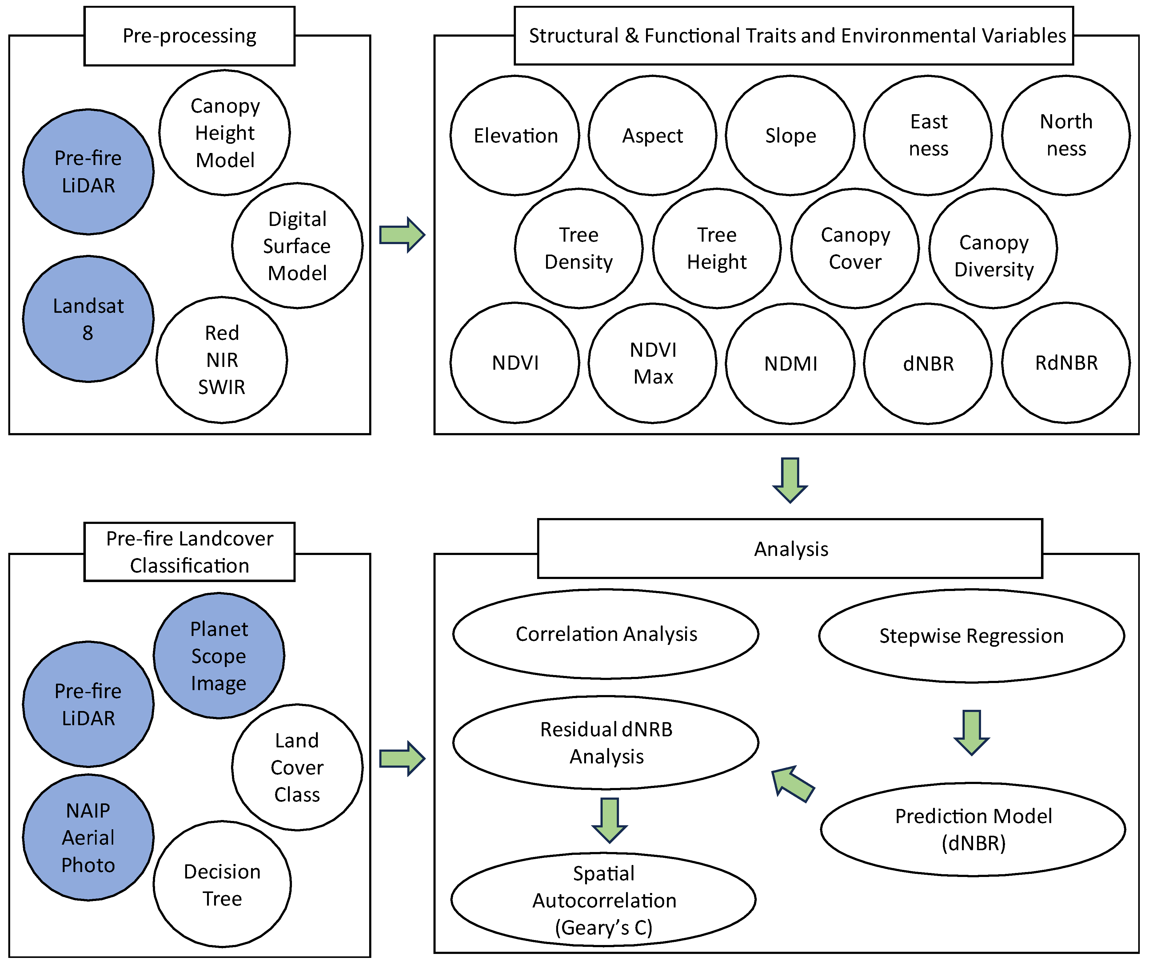
2.2. Vegetation Structural and Topographical Variables Derived from Aerial LiDAR

Figure 2 shows the workflow and data sources, processing, and analysis steps that were performed to conduct this research. The study utilized a pre-fire LiDAR dataset obtained from the USGS 3DEP, which meets the quality standard of level 2 (0.7 nominal pulse spacing, NPS) and has an average point density of 2 points per square meter. The lidR package in R was employed to extract individual trees from the point cloud [47]. Using the package, we executed a sequence of processing steps including ground classification [48], digital terrain and surface model (DEM) generation [49], height normalization, canopy height model (CHM) generation [50], and individual tree segmentation [51]. Elevation, slope, aspect, eastness and northness were derived from the LiDAR data, as shown in the below (Equations (1)–(4)):

$$Slope\left(degrees\right)=ATAN\left(\sqrt{({dz/dx)}^2+({dz/dy)}^2}\right)\times 57.29578$$

(1)

$$Aspect=\left(57.29578-\mathrm{A}\mathrm{T}\mathrm{A}\mathrm{N}2([dz/dy]-[dz/dx]\right))$$

(2)

$$Eastness=Sin\left(Aspect\right)$$

(3)

$$Northness=Cos\left(Aspect\right)$$

(4)

DEM data allow for the direct calculation of slope and aspect by analyzing the infinitesimal changes in elevation $\left(dz\right)$ along the x and y cell directions ($dx,dy)$ within the dataset. Eastness is determined by computing the sine of the aspect, revealing the east-to-west orientation of the slope, while northness is derived from the cosine of the aspect, indicating the north-to-south orientation of the slope [52].

CHM generation in LiDAR deploys triangulation-based algorithms that differ from point-to-raster algorithms. While point-to-raster algorithms are straightforward and enable user-defined resolution, they may produce empty pixels when the grid resolution is too fine for the available point density [47]. In contrast, triangulation-based algorithms utilize a Delaunay triangulation to interpolate first returns, which is more intricate but eliminates empty pixels irrespective of the input data resolution.

Tree density, tree height, canopy cover, and canopy diversity (standard deviation of canopy height) are estimated from a 1-m CHM, which is adopted by the individual tree segmentation (ITS) method [53]. To calculate tree density, tree top points are identified directly from the straightforward method from the CHM and canopy coverage [54]. These methods operate on the premise that the apex of a tree is the tallest point within its crown, and the crown’s periphery is comparatively lower [55]. A local maximum (LM) filter, typically with a designated size sliding window, is employed in a CHM, derived from a point cloud to pinpoint LMs that indicate treetops [56]. Despite the perceived challenge of CHM-based techniques in identifying overshadowed trees, they can serve as initial points for algorithms that outline tree crowns in a CHM or point cloud space [57]. Information for each treetop was recognized as a point feature and transformed into density features once placed on a grid with a 30 m × 30 m fishnet pattern. This was conducted to facilitate a comparison with the burn severity derived from the Landsat 8 data. Each tree height estimate can be used to indicate canopy diversity by calculating the standard deviation of each tree height in the grid [58].

2.3. Spectral Indices to Derive Burn Severity and Vegetation Functional Variables Using Satellite Imagery

Satellite-derived burn severity data are typically quantified by spectral changes between the pre-and post-fire satellite images. We acquired Landsat 8 satellite images of the study area for 14 July 2019 and 1 August 2020, which represent the pre- and post-fire conditions, respectively. There is an active debate regarding which of the two main equations, the delta normalized burn ratio (dNBR) and its relativized form (RdNBR), or other newer formulations (RBR) is most suitable for quantifying burn severity [59]. We used fire severity indices generated from multi-date LANDSAT data, published by the Burned Area Emergency Response (BAER) program at the Geospatial Technology and Applications Center in the USDA Forest Service. The program released normalized burn ratio (NBR) and dNBR burn severity datasets based on Landsat 8 imagery. The RdNBR index is available through RAVG (Rapid Assessment of Vegetation Condition after Wildfire), which was published in Aug 2021, one year after fire containment [60,61,62].

Burn ratio calculations are based on the NBR index. The NBR uses near-infrared (ρNIR) and shortwave infrared (ρSWIR) spectral reflectance data to highlight the difference between healthy vegetation (which reflects NIR radiation strongly and absorbs SWIR radiation) and burned areas (which reflect both types of types of radiation more evenly) [62]. The NBR is calculated using the following formula:

$$NBR=\left(\mathsf{\rho }NIR-\mathsf{\rho }SWIR\right)/(\mathsf{\rho }NIR+\mathsf{\rho }SWIR)$$

The NBR values range from −1 to 1. A value of −1 indicates the absence of vegetation such as in areas severely affected by fire. On the other hand, a value of 1 indicates areas with dense vegetation with no reduction in reflectance. The differenced NBR (dNBR), which is adjusted with the amount of pre-fire vegetation, is calculated using the following formula and has a broader range (−2 to +2):

$$dNBR=\left(PreNBR-PostNBR\right)\times 1000$$

Sites that have experienced severe burning are represented by high positive values within this range (

Table 1. Description of burn severity based on the magnitude of landscape changes [8].

Burn Severity	$\mathbf{dNBR}\mathbf{Range}\left(\mathbf{Scaled}\mathbf{by}{10}^3\right)$	Ecological Description
Unchanged	−100 to +99	Indicates that the area one year after the fire was indistinguishable from pre-fire conditions. This may indicate that the area did not burn.
Low	+100 to +269	Areas of surface fire with little change in cover and little mortality of the structurally dominant vegetation.
Moderate	−270 to +659	A mixture of effects on the structurally dominant vegetation.
High	+660 to +1300	Areas of high to complete mortality of the dominant vegetation.

). It would be biased in areas with low pre-fire biomass, where even a high-severity fire might result in a low dNBR simply because there was not much vegetation to burn in the first place. In this study area, the area already burned by previous fire would be biased when only using dNBR. To address this issue, the relativized differenced NBR (RdNBR) normalizes the dNBR by the square root of the pre-fire NBR. This normalization reduces the bias in the dNBR, making the RdNBR a more accurate measure of burn severity in areas with low pre-fire biomass [59]. The relative dNBR is computed by applying an offset and a scale factor to the dNBR [62]:

$$RdNBR=dNBR/\sqrt{\left|(\mathrm{P}\mathrm{r}\mathrm{e}\mathrm{N}\mathrm{B}\mathrm{R}/1000\right|)}$$

The RdNBR is a measure of the change in burn severity relative to the amount of vegetation that was present before the fire. This generally provides a more representative measure of the actual impact of the fire on the landscape [61].

To understand the functional traits of the mountain ecosystem, we calculated the pre-fire normalized difference vegetation index (NDVI) and normalized difference moisture index (NDMI) using red, NIR, and SWIR reflectance values. These vegetation indices are commonly used to characterize plant health, biomass, and water content [63]. These indices quantify the density and greenness of vegetation based on the difference in reflectance between the near-infrared (NIR) and red bands of the electromagnetic spectrum. It has been suggested that shortwave infrared is well-suited for the remote sensing of the canopy water content [64]. Consequently, it might also reflect the pre-fire canopy conditions [65].

By analyzing the NDVI and NDMI values of an area before a fire, we can understand the baseline vegetation conditions when comparing them with structural traits from a LiDAR dataset and quantify how these vegetation and structural variables interact with each other to affect the burn severity. The indices were derived from Landsat 8 satellite imagery from the pre-fire scene in July 2019, prior to the 2020 Bighorn Fire, and were calculated using the following formula:

$$NDVI=\frac{\mathsf{\rho }NIR-\mathsf{\rho }Red}{\mathsf{\rho }NIR+\mathsf{\rho }Red}$$

$$NDWI=\frac{\mathsf{\rho }NIR-\mathsf{\rho }SWIR}{\mathsf{\rho }NIR+\mathsf{\rho }SWIR}$$

The highest NDVI of 2019, a year prior to the fire, was determined by comparing the mean NDVI values over the year using Landsat 8 images of the boundary of the burned area. This analysis was performed through Google Earth Engine. The maximum index was included to represent the fuel loads and vegetation conditions before the fire. As a result, the Landsat 8 image from 2 October 2019, displays the peak mean NDVI value for the region. All spectral indices used in the analysis are shown in Figure 2.

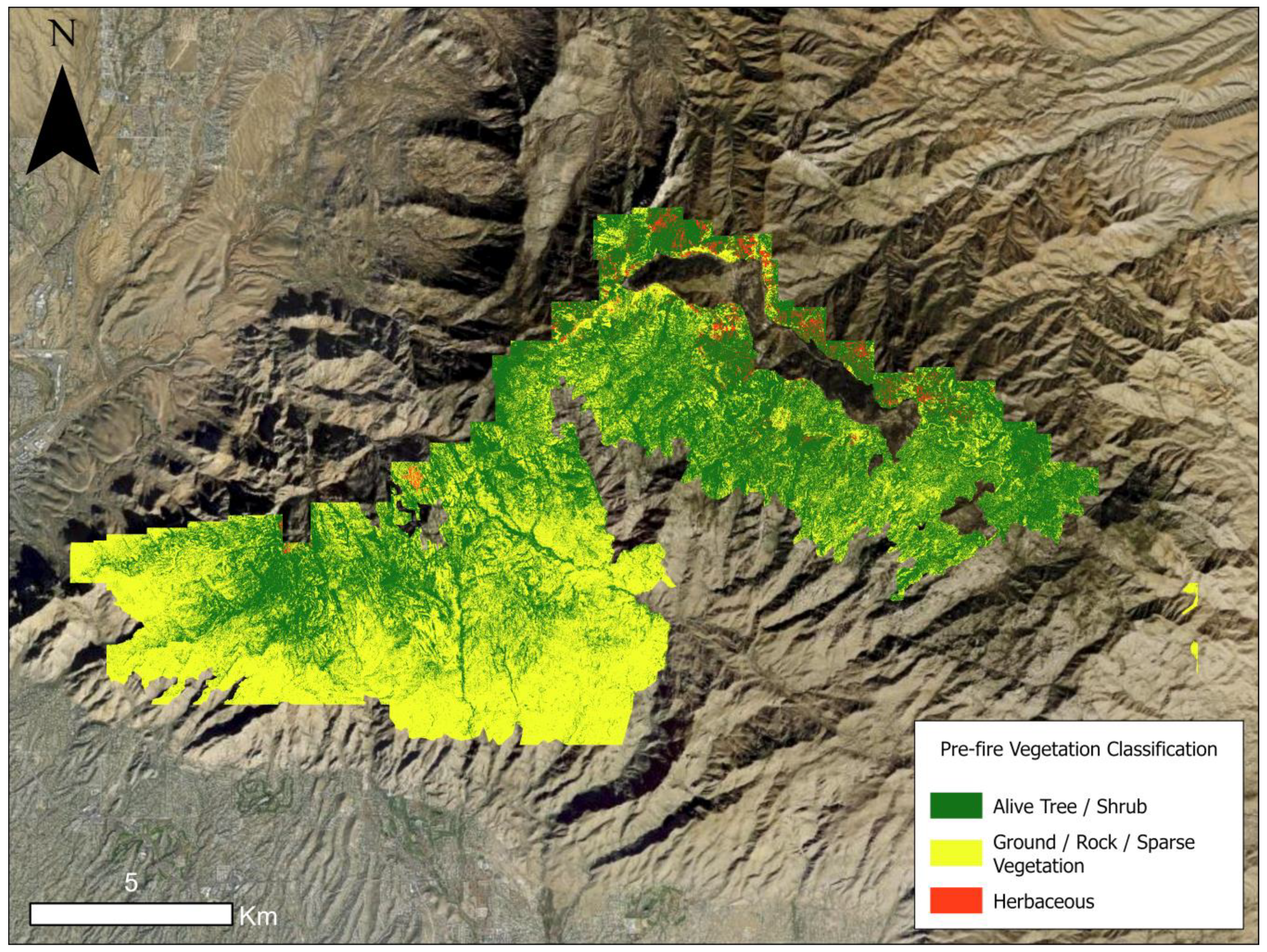
2.4. Pre-Fire Land Cover Classification

Burn severity is significantly influenced by pre-fire environmental conditions, with a particular emphasis on land cover. As illustrated in Figure 1, a substantial portion of the study area had experienced multiple previous fires, leading to varying rates of recovery across different locations. Consequently, we used thematic land cover classification results to represent the pre-fire conditions of the forest.

To conduct thematic imagery classification and estimate basic land cover categories throughout the entire SCMs over a pre-fire time series, we employed a combination of passive and active remote sensing data sources (Figure 2). These sources included Planet Scope satellite images (4-band, 3-m resolution) and the USGS 3DEP LiDAR canopy height model. The Planet Scope satellite imagery was chosen for its frequent temporal coverage before as well as its relatively high spatial resolution of 3 m, surpassing that of Landsat 8.

We utilized pre-fire aerial LiDAR data to generate canopy height models for use as input in our classification process. Our approach involved employing these remote sensing data sources in a supervised thematic classification task, wherein individual pixels were categorized as belonging to either a vegetation or abiotic feature type. To accomplish this, we utilized the C5.0 decision tree classifier algorithm, implemented within RStudio, to assign pixels into one of four distinct classes (

Table 2. Thematic classes for vegetation cover classification.

Thematic Classes	Feature Properties
Alive Tree/Shrub	Green vegetation spectral signature and have heights associated with it (>1 m height).
Bare Ground/Rock/ Sparse Vegetation	No green vegetation spectral signature and do have low canopy heights (<1 m height).
Dead Tree/Shrub	No green vegetation spectral signature, but do have canopy heights (>1 m height).
Herbaceous	Green vegetation spectral signature but have low height (<1 m). This includes green grasses, forbs, and ferns.

).

Decision trees represent a class of supervised learning algorithms employed extensively for the purposes of both classification and regression [66]. The C5.0 algorithm employs an iterative, top-down, and recursive approach in the construction of decision trees [67]. This method initiates the process by designating the entire dataset as the root node of the tree and subsequently divides the data into subsets based on the attributes or features, seeking to optimize the maximization of information gain or minimization of impurity as its guiding principle. In the context of our study, this functionality of C5.0 was harnessed to effectuate the classification of distinct land cover classes with the overarching goal of maximizing the information gain across these varying categories.

Given the acknowledged risk of overfitting stemming from an imbalanced distribution of samples [68], we adopted a training-validation sample ratio of 75% to 25% for each class. Additionally, we employed 58 reference points distributed across the study area to assess the overall accuracy of the final classification outcome. The land cover data were a crucial factor in quantifying the regression results, enabling us to discern variations in these results based on the attributes of the land cover classification outcomes.

2.5. Correlation Analysis and Stepwise Regression Using Mallow’s C(p)

We employed Pearson correlation analysis to investigate the interrelations among various environmental factors (Figure 2). We used hierarchical clustering based on correlation coefficients among these variables based on the coefficient of correlation among the environmental variables. This analytical approach facilitated the discernment of linear relationships among paired variables. Moreover, it assisted in selecting the burn severity index (be it RdNBR or dNBR) that most accurately encapsulated the dominant trends and relationships within the dataset.

We used stepwise regression as a statistical method to select a subset of relevant predictor variables from a larger set of variables in a linear regression model. The objective was to identify a subset of predictors that would optimally explain the variation in the response variable while maintaining model simplicity [69]. The leaps package in R provided tools to perform stepwise regression with different selection criteria such as the Akaike information criterion (AIC) or Bayesian information criterion (BIC) [70]. We used this routine to perform stepwise regression, exhaustively exploring all possible combinations of predictor variables to identify the best subset based on the selected criterion (AIC or BIC). The best subset was the one that provided the best trade-off between model fit and complexity. We evaluated the best combination of regression model using Mallows’ Cp, also known as “Mallow’s C(p)” statistic [71,72], which measures the predictive accuracy used in the context of linear regression and model selection. It is used as part of the process for selecting the best subset of predictor variables in stepwise regression. The purpose of Mallows’ Cp is to assess the goodness-of-fit of a model while considering its complexity. It is particularly useful when comparing different subsets of predictor variables in stepwise regression, where subsets with different numbers of predictors are evaluated.

The formula for Mallows’ Cp statistic is as follows:

$$C_p=\left(\frac{SS{E}_p}{{\sigma }^2}\right)-\left(n-2p\right)$$

where:

• $S{EE}_p$ is the sum of squared errors (residual sum of squares) for the model with p predictor variables;
• ${\sigma }^2$ is the estimated error variance for the full model (model with all predictor variables);
• n is the number of observations in the data;
• p is the number of predictor variables in the model.

Mallow’s Cp value is contingent upon the variance between the anticipated error of a model with p predictors and the error variance of the complete model. A lower Mallows’ Cp value signifies an optimal balance between the model’s fit and complexity. When the Cp value is proximate to, or slightly exceeds, the number of predictors (p), it indicates a model that strikes a balance between complexity and simplicity. In our research, we examined many environmental variable combinations to identify the most suitable regression model that could account for variation in fire severity using this criterion.

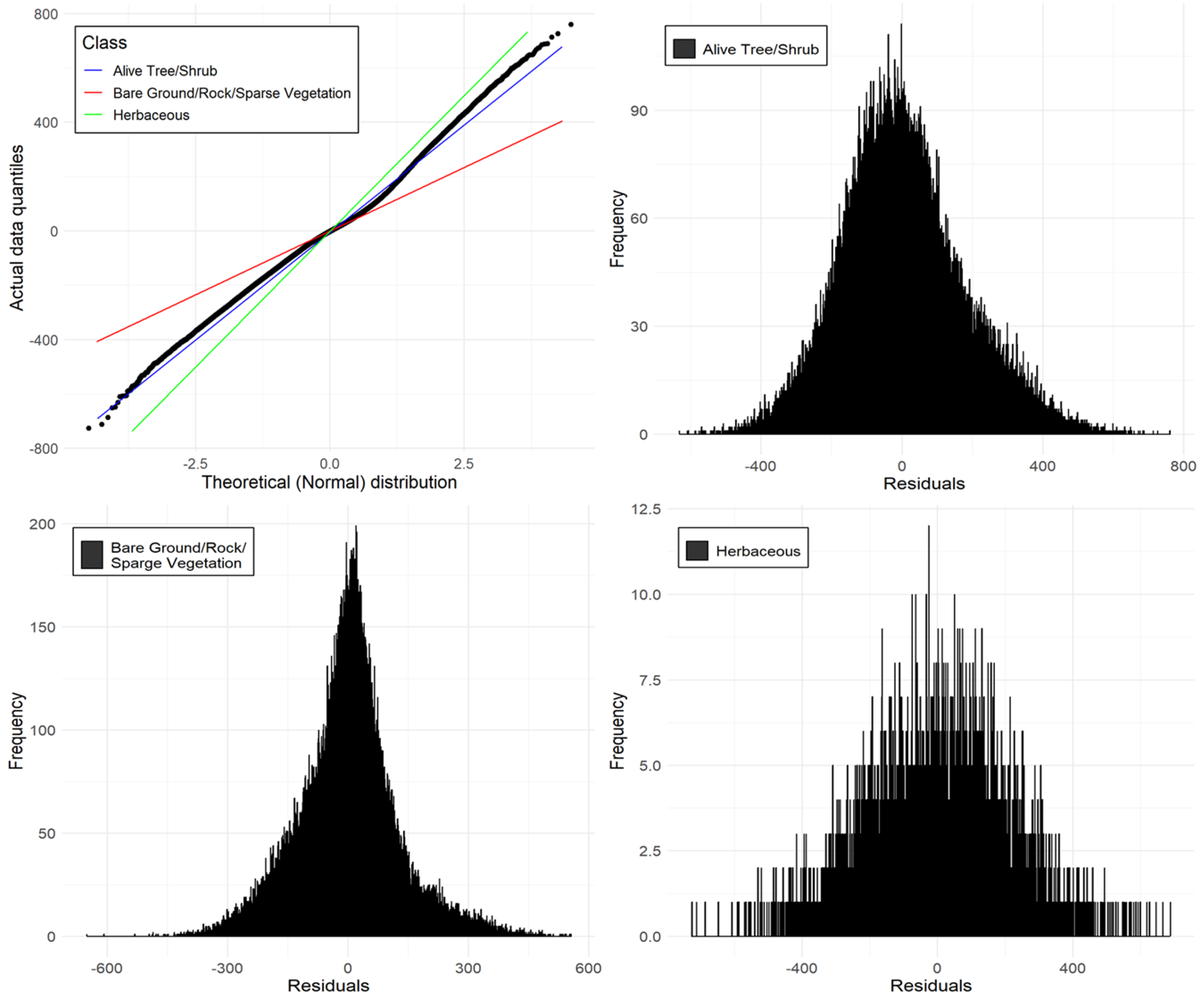
2.6. Analyzing Residual Values with Geary’s C

We used the regression model results to compute the residual values for dNBR, which represent the difference between the estimated burn severity value obtained from the stepwise regression model and the actual burn severity value derived from the Landsat satellite data (Figure 2). These residual values exhibit natural autocorrelation, as described by Legendre [73], due to the inherent spatial autocorrelation in ecological data. Spatial autocorrelation in burn severity arises because species at one location are strongly influenced by both biotic and abiotic factors, which tend to be spatially coherent over a landscape area.

Since wildfires cannot be replicated, it is crucial to maximize the number of data points (N) and implement blocking within burn severity categories to ensure that our statistical analysis yields valuable insights without being affected by pseudoreplication or spatial autocorrelation. This challenge is further complicated by landscape heterogeneity, which varies depending on the scale of analysis [74]. Therefore, our approach in this study involved analyzing all residuals to identify potential autocorrelation patterns, rather than relying on small plots that may not adequately capture such autocorrelation.

Global Moran’s I and Geary’s C are spatial autocorrelation coefficients used to assess the degree of spatial dependency among observations in geographical space [75]. Global Moran’s I quantifies the overall spatial autocorrelation within a dataset, indicating whether adjacent observations tend to exhibit similar (positive autocorrelation) or dissimilar (negative autocorrelation) values [76]. While both metrics evaluate spatial autocorrelation, they exhibit differences in sensitivity and focus. Moran’s I is generally more suitable for capturing global spatial trends, while Geary’s C tends to be more responsive to local spatial patterns and variations because it utilizes the sum of squared distances, in contrast to Moran’s I, which relies on standardized spatial covariance [77]. Geary’s C, due to its use of squared distances, is less influenced by linear associations and may detect autocorrelation that Moran’s I might underweight [77]. These two coefficients offer complementary insights into the underlying spatial structures and dependencies inherent in geographical data. In this study, we employed Geary’s C to quantify the spatial pattern of residual values in relation to the final coefficient of determination obtained from the stepwise regression analysis.

3. Results

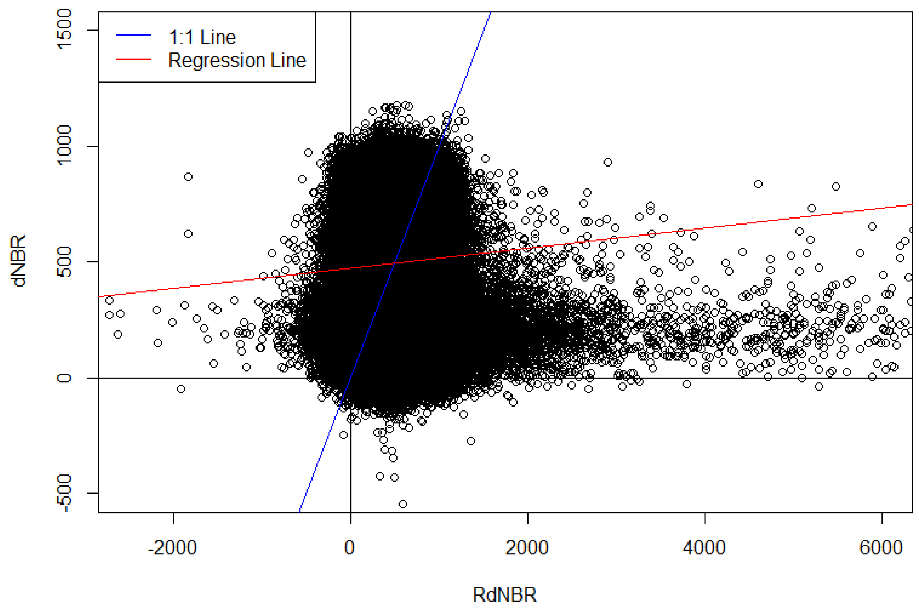
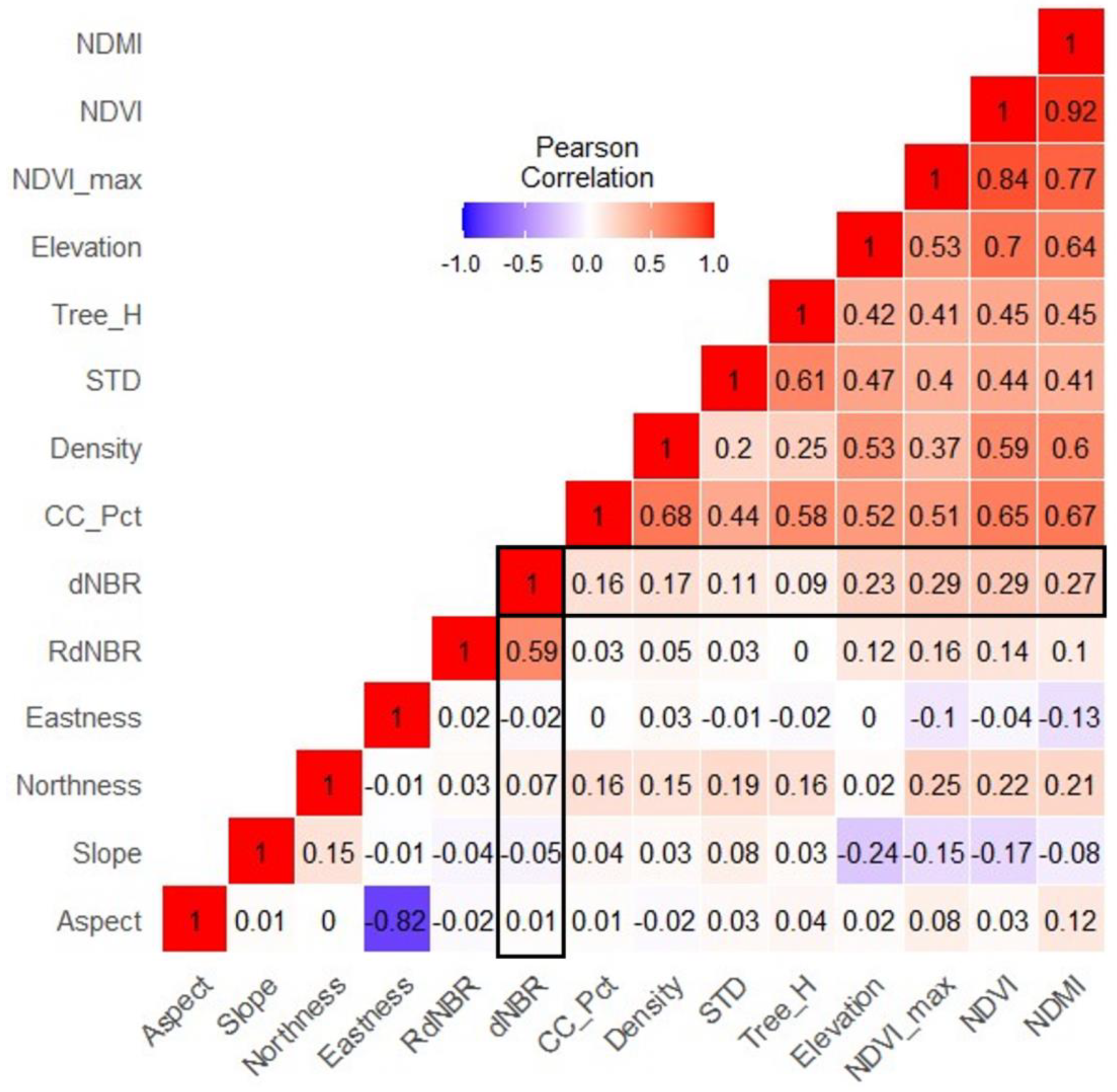
3.1. Correlation between Environmental Variables and Burn Severity Indices

The relationship between RdNBR and dNBR from Landsat 8 images in 2020 was generally linear (Figure 3), with some outliers exceeding index values of 2000. Positive dNBR values signified a rise in near-infrared radiation reflectance post-fire compared to its pre-fire state. For both dNBR and RdNBR, most areas exhibited positive values.

We found a robust correlation (r = 0.83) between the two burn severity indices, RdNBR and dNBR. This implies that employing either index for regression analysis might produce analogous outcomes. Vegetation indices manifest higher correlation coefficients, in contrast to the lower coefficients among terrain attributes such as eastness or northness (Figure 4). Notably, elevation emerged as a pivotal variable correlating with alterations in the vegetation indices (r = 0.85 with NDVI and r = 0.78 with NDMI). This may be attributed to the properties of the study locale, often referred to as a “Sky Island”, which possesses clines in abundance of vegetation and fuel along the elevation gradient [36,78]. In contrast, when comparing the burn severities with all other environmental variables, dNBR consistently exhibited higher correlation coefficients compared to the RdNBR across nearly all variables. Thus, dNBR appears to better represent the entire set of variables.

3.2. Stepwise Regression Analysis Using Land Cover Classification Results

The transitional zone (Figure 5), which lies between elevations of 1500 to 1800 m and is characterized by yellow and light blue colors, was previously affected by the Aspen Fire in 2003. The vegetation of this area is a mix of desert, woodland, and montane plants, many of which recovered during the post-fire era after the Aspen Fire. However, the northeast side of the mountain, which is highlighted by the red and orange colors in Figure 5, was previously damaged in 2002 by the Bullock Fire and showed more difference compared to the mid-elevation transition area. This area is mostly classified as a mixed-conifer and subalpine forest range, covered by tall trees.

Considering the heterogeneous vegetation coverage within the study area, we evaluated areas with diminished residual values in a regression model. To gauge the sensitivity of dNBR to various environmental factors, we developed a stepwise regression model with dNBR values as the dependent variable and 13 other environmental factors as independent variables to elucidate disparities in the residual values amongst the groups.

The results show that different types of land cover contained different combinations of important variables in the stepwise regression model (

Table 3. Stepwise regression model result based on land cover classification. The significance of variables depends on differences in cover types; not all variables are always significant. (* indicates significance, p < 0.05).

Land Cover	Alive Tree/Shrub	Ground/Rock/Sparse Vegetation	Herbaceous	AllL and Cover
Slope	*	*
Aspect				*
NDVI	*	*	*	*
Canopy Cover	*	*	*	*
NDMI	*		*	*
Northness
Eastness	*	*
NDVI_Max	*		*	*
Elevation		*	*	*
Tree Density	*	*	*	*
Standard Deviation of Canopy Height	*	*	*
Tree Height		*	*	*
${\mathit{R}}^2$	0.30	0.28	0.29	0.36

).

Vegetation-associated indices and variables including the NDVI prior to the fire, canopy cover, tree density, and the standard deviation of tree height were significantly associated with burn severity across all land cover types. However, variables such as the NDMI and the maximum NDVI (NDVI_Max) did not exhibit a significant relationship with burn severity within areas covered by healthy vegetation. In unclassified land cover areas, aspect was incorporated within the amalgamation of variables within the stepwise regression model. Because most of the study area has a south-facing slope, the variable northness was not significantly correlated with burn severity of the Bighorn Fire across any classifications. Given the considerable discrepancy in sample sizes amongst the herbaceous (n = 4249), ground (n = 68,754), and alive tree (n = 65,611) areas, a direct comparison was not feasible.

Correlation analysis indicates that NDVI exhibited the strongest correlation with changes in dNBR. Additional comparisons emerged when contrasting the outcomes of the regression model solely utilizing NDVI with those of the stepwise model. A simple linear regression analysis encompassing all land cover types using only NDVI as the predictor variable produced a lower coefficient of determination (r²) compared to the coefficient derived from the stepwise model. Specifically, the coefficient obtained from the model employing solely NDVI was 0.33, compared to 0.16 for herbaceous cover, 0.26 for ground, and 0.25 for the live vegetation area. In general, these coefficients were marginally low; however, we noted more pronounced disparities in the case of the herbaceous area compared to the other two land cover categories.

The outcomes derived from the stepwise regression analysis indicated a notable association between all environmental variables and the dNBR burn severity index (Table 3). Each land cover type exhibited a comparable coefficient of determination, yielding a value of 0.30, while the significant variables within the stepwise regression model varied among the cover types. Notably, NDVI, canopy cover, and tree density emerged as significant variables across all land cover types, underscoring their substantial influence on burn severity outcomes. Consistent with findings from the correlation analysis, vegetation-related variables such as NDVI prominently featured in the stepwise regression, whereas terrain variables such as slope and aspect demonstrated a negligible impact on burn severity, at least within the context of this study.

The frequency and spatial distribution of the residual values derived from the regression models were specific to three distinct land cover types (Figure 6 and Figure 7). These residual values elucidate the disparities between the predicted and observed burn severity indices. In Figure 6, the distribution of residual values across all classes demonstrated adherence to a normal distribution, as evidenced by their alignment with the theoretical quantiles. These quantiles were calculated based on the assumed parameters of the distribution such as mean and standard deviation. However, deviations from this expected pattern were observed among the three different land cover classes. The residual values associated with the alive trees and shrubs class exhibited a departure from the expected straight line, indicating a discrepancy between the predicted and observed values. Conversely, the herbaceous class displayed a downward trend, suggesting lighter tails, while the bare ground/rock/sparse vegetation class exhibited an upward trend, indicative of heavier tails.

Figure 7 provides a spatial representation of these residual value patterns. Elevated regions tended to display higher residual values, correlating with more severe burn severity indices. Lower elevation areas showed minimal differences between the predicted and observed residual values. These spatial trends aligned with the terrain characteristics of the sky island; areas of higher elevation typically featured larger biomass coverage, whereas lower elevation areas were characterized by shrubs and bare ground.

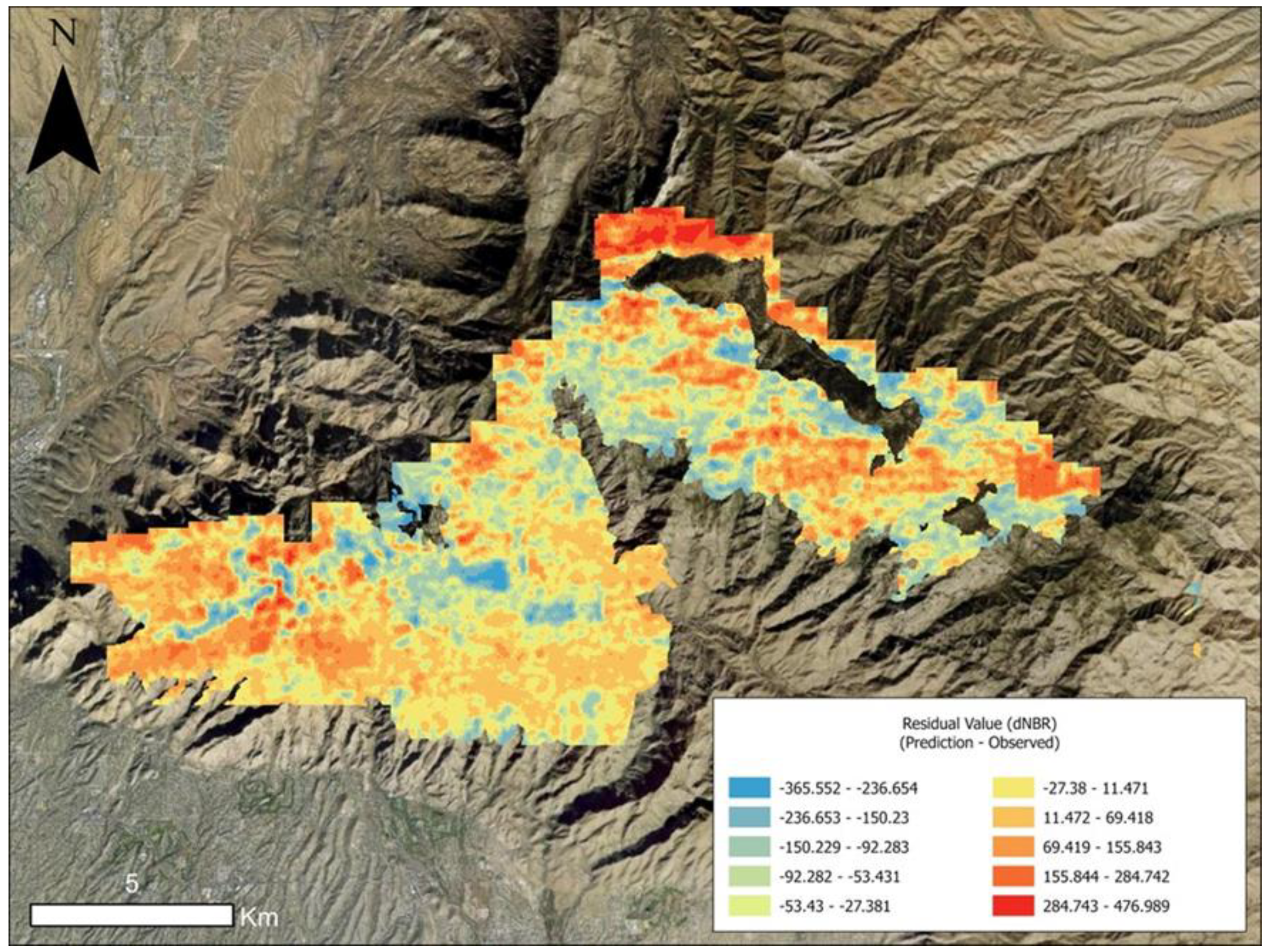
3.3. Calculating Spatial Distribution Using Geary’s C

To ascertain the relationship between the residual values and land cover types, we evaluated the spatial autocorrelation within the dataset. The absence of spatial autocorrelation implies that the residual values were randomly distributed without interdependencies among the neighboring data points. Given that the land cover data indicated areas of homogeneous or similar cover types, we anticipated the presence of spatial autocorrelation within the dataset.

In the present study, Geary’s C was computed to evaluate the spatial characteristics of the residual values, specifically investigating the presence or absence of spatial autocorrelation. Given that each set of residual values was derived from distinct regression models, each corresponding to a specific land cover type, we anticipated that spatial autocorrelation would manifest across all classes (

Table 4. Comparison of spatial autocorrelation between land cover types.

Land Cover	Geary’s C	Expectation	Variance	p-Value
Live vegetation	185.9120	0.5192856	1	0
Ground	134.4589	0.6440652	1	0
Herbaceous	55.8227	0.4406085	1	0

). All Geary’s C values were notably larger than 1, suggesting a strong negative spatial autocorrelation within each category.

4. Discussion

When comparing dNBR and RdNBR through the distribution plots, we found that dNBR exhibited fewer outlier values in the examined study area. The results indicate that dNBR generally aligned more closely with the actual burn severity than the RdNBR for this area. However, as previously mentioned, the accuracy can fluctuate based on various environmental factors. While this study primarily examined the correlation between burn severity and pre-fire conditions, future research could benefit from comparing the burn severity to the actual changes in biomass. Such an investigation could shed light on the effectiveness of different burn severity indices in environments like sky islands, characterized by a diverse gradient of pre-fire vegetation types and structures with variable fire return histories.

Through our correlation and regression assessments, we found that certain vegetation and biomass attributes exhibited a stronger relationship with burn severity compared to other factors such as terrain. Prior research primarily concentrated on evaluating the fuel structure and loading solely through the utilization of dNBR indices [79], in contrast to the present investigation, which integrated an expanded array of structural and functional variables encompassing terrain and canopy attributes. Despite the relatively diminished overall predictive precision concerning the potential burn severity discerned within this study, it offers a means of identifying variables with greater likelihoods of predicting the burn severity. Additionally, the predictive accuracy exhibited variability, contingent upon the distinct ecosystem types that typify diverse landscapes [80,81]. This study delineated the distinctive attributes of sky islands in the southwestern United States, characterized by a blend of vegetation amidst rugged mountainous terrain.

It is axiomatic that regions with more vegetation inherently have more fuel, leading to heightened burn indices [82]. Previous studies have shown that densely forested areas with conifer trees have a higher regression value, while Mediterranean shrublands have a lower one. Generally, the correlation coefficient ($r^2$) for NDVI and dNBR values ranges from 0.5 to 0.8 [62,83,84]. Given that our study zone encompassed a range from shrublands to thick forests situated on steep terrain, the derived $R^2$ value of 0.358 might appear counterintuitive at first glance. In a corresponding investigation, specifically in the context of a comparative analysis involving a field-based fire severity index (GeoCB)I and dNDVI derived from Landsat TM data, the $R^2$ value fell within the range of 0.3 to 0.5, aligning closely with the outcomes obtained within the present study [85]. Nevertheless, the precise regression value can fluctuate based on various determinants such as the nature of pre-fire vegetation, burn severity, and the specific remote sensing equipment utilized.

The study indicates that the residuals of the stepwise regression model exhibit spatial variability across mountainous terrains. As the elevation increased, there was a marked increase in the residual values. This trend aligns closely with the inherent attributes of sky island mountains. Specifically, regions at lower elevations consist predominantly of sparse shrublands, while higher elevations are characterized by a dense canopy of coniferous trees. Notably, an intriguing pattern discerned from the vegetation classification map indicates a prevalence of herbaceous species at higher elevation areas. These herbaceous regions overlapped predominantly with zones that experienced previous fire events, notably the Bullock and Aspen Fires, indicating a possible post-fire community. Residual errors tended to be lower in proximity to these herbaceous zones in comparison to densely forested areas, even at comparable elevations.

Accurate discrimination between rocks and exposed terrain presented inherent challenges, necessitating their amalgamation into a unified classification category. Notably, the discernment of sparse vegetative features, particularly arid shrubs lacking pronounced green pigmentation, proved to be a formidable task, with heightened complexity observed at lower elevations within the cartographic representation. Consequently, the category encompassing sparse vegetation was amalgamated with the class designated for bare ground and rock. We acknowledge the potential for the occasional misclassification of isolated boulders as deceased arboreal or shrub entities.

5. Conclusions

This study presented a novel approach for investigating the predictability of post-fire burn severity using pre-fire structural and functional vegetation traits. We leveraged a well-established regression model retrospectively to identify a viable methodology for such predictions. Among the various factors analyzed, vegetation attributes emerged as the most significant predictors of burn severity. Stepwise regression analysis revealed that vegetation-related indices, NDVI, canopy cover, and tree density were significant variables across all land cover types. These variables were highly correlated with burn severity values throughout the mountain range. In the scope of fire behavior, NDVI acts as a proxy for essential functional traits influenced by drought conditions, and tree density and canopy-related variables reflect the available fuel loads in the mountain ranges. It also implies that the areas with denser vegetation and higher levels of greenness in this mountain range had experienced more severe burns. It is worth noting that the study sites have a history of multiple fires, resulting in more diverse environmental conditions compared to other potential areas. Despite this, we successfully extracted variables indicative of functional traits from the LiDAR and satellite datasets, demonstrating valuable methods for future research in this direction.

Not all study locales consistently furnish adequate geospatial data, thus imposing limitations on the evaluation of post-fire severity. Nevertheless, the judicious adoption of the stepwise regression methodology, as demonstrated in this investigation, offers a viable means to retroactively estimate the impact of pre-fire conditions on post-fire burn severity by utilizing widely accessible satellite datasets such as Landsat or CubeSat. In this framework, these findings underscore that a comprehensive array of pre-fire vegetation structural, functional, and environmental variables can effectively facilitate the estimation of burn severity. However, caution must be exercised in extrapolating these methodologies to other regions and ecosystem types, as variations in tree species and terrain characteristics necessitate nuanced adaptations.

While this study examined numerous variables, the advent of newly developed sensors and satellites promises a wealth of additional information. It is imperative, however, to scrutinize these advances to learn more about what they may tell us regarding the factors that govern burn severity and ascertain the extent of their influence, particularly amidst the backdrop of recent extreme climate patterns in the southwestern United States. These insights not only augment our comprehension of burn severity dynamics, but also catalyze further inquiry in this field, thereby fostering advancements in both knowledge and methodology.

References

1. Keeley, J.E.; van Mantgem, P.; Falk, D.A. Fire, climate and changing forests. Nat. Plants 2019, 5, 774–775. [Google Scholar] [CrossRef] [PubMed]
2. DeBano, L.F.; Neary, D.G.; Ffolliott, P.F. Fire Effects on Ecosystems; John Wiley & Sons: Hoboken, NJ, USA, 1998. [Google Scholar]
3. Davis, K.T.; Dobrowski, S.Z.; Higuera, P.E.; Holden, Z.A.; Veblen, T.T.; Rother, M.T.; Parks, S.A.; Sala, A.; Maneta, M.P. Wildfires and climate change push low-elevation forests across a critical climate threshold for tree regeneration. Proc. Natl. Acad. Sci. USA 2019, 116, 6193–6198. [Google Scholar] [CrossRef] [PubMed]
4. Dove, N.C.; Safford, H.D.; Bohlman, G.N.; Estes, B.L.; Hart, S.C. High-severity wildfire leads to multi-decadal impacts on soil biogeochemistry in mixed-conifer forests. Ecol. Appl. 2020, 30, e02072. [Google Scholar] [CrossRef] [PubMed]
5. Rengers, F.K.; Tucker, G.E. The evolution of gully headcut morphology: A case study using terrestrial laser scanning and hydrological monitoring. Earth Surf. Process. Landf. 2015, 40, 1304–1317. [Google Scholar] [CrossRef]
6. Broxton, P.D.; van Leeuwen, W.J.D.; Biederman, J.A. Forest cover and topography regulate the thin, ephemeral snowpacks of the semiarid Southwest United States. Ecohydrology 2020, 13, e2202. [Google Scholar] [CrossRef]
7. Collins, B.M.; Fry, D.L.; Lydersen, J.M.; Everett, R.; Stephens, S.L. Impacts of different land management histories on forest change. Ecol. Appl. 2017, 27, 2475–2486. [Google Scholar] [CrossRef] [PubMed]
8. Keeley, J.E. Fire intensity, fire severity and burn severity: A brief review and suggested usage. Int. J. Wildland Fire 2009, 18, 116–126. [Google Scholar] [CrossRef]
9. Conard, S.G.; Sukhinin, A.I.; Stocks, B.J.; Cahoon, D.R.; Davidenko, E.P.; Ivanova, G.A. Determining Effects of Area Burned and Fire Severity on Carbon Cycling and Emissions in Siberia. Clim. Chang. 2002, 55, 197–211. [Google Scholar] [CrossRef]
10. Shive, K.L.; Preisler, H.K.; Welch, K.R.; Safford, H.D.; Butz, R.J.; O‘Hara, K.L.; Stephens, S.L. From the stand scale to the landscape scale: Predicting the spatial patterns of forest regeneration after disturbance. Ecol. Appl. 2018, 28, 1626–1639. [Google Scholar] [CrossRef]
11. Key, C.; Benson, N. Landscape assessment: Ground measure of severity, the Composite Burn Index; and remote sensing of severity, the Normalized Burn Ratio. FIREMON Fire Eff. Monit. Inventory Syst. 2005, 2004, LA1–LA51. [Google Scholar]
12. Fernandes, P.M.; Rigolot, E. The fire ecology and management of maritime pine (Pinus pinaster Ait.). For. Ecol. Manag. 2007, 241, 1–13. [Google Scholar] [CrossRef]
13. Veraverbeke, S.; Rogers, B.; Randerson, J. Daily burned area and carbon emissions from boreal fires in Alaska. Biogeosciences 2015, 12, 3579–3601. [Google Scholar] [CrossRef]
14. Jones, B.M.; Kolden, C.A.; Jandt, R.; Abatzoglou, J.T.; Urban, F.; Arp, C.D. Fire Behavior, Weather, and Burn Severity of the 2007 Anaktuvuk River Tundra Fire, North Slope, Alaska. Arct. Antarct. Alp. Res. 2009, 41, 309–316. [Google Scholar] [CrossRef]
15. Miller, R.F.; Chambers, J.C.; Pyke, D.A.; Pierson, F.B.; Williams, C.J. A Review of Fire Effects on Vegetation and Soils in the Great Basin Region: Response and Ecological Site Characteristics; General Technical Report RMRS-GTR-308; US Department of Agriculture, Forest Service, Rocky Mountain Research Station: Fort Collins, CO, USA, 2013; Volume 308. [Google Scholar]
16. Schwilk, D.W.; Caprio, A.C. Scaling from leaf traits to fire behaviour: Community composition predicts fire severity in a temperate forest. J. Ecol. 2011, 99, 970–980. [Google Scholar] [CrossRef]
17. Lee, B.; Kim, S.Y.; Chung, J.; Park, P.S. Estimation of fire severity by use of Landsat TM images and its relevance to vegetation and topography in the 2000 Samcheok forest fire. J. For. Res. 2008, 13, 197–204. [Google Scholar] [CrossRef]
18. García-Llamas, P.; Suárez-Seoane, S.; Taboada, A.; Fernández-Manso, A.; Quintano, C.; Fernández-García, V.; Fernández-Guisuraga, J.M.; Marcos, E.; Calvo, L. Environmental drivers of fire severity in extreme fire events that affect Mediterranean pine forest ecosystems. For. Ecol. Manag. 2019, 433, 24–32. [Google Scholar] [CrossRef]
19. Viedma, O.; Quesada, J.; Torres, I.; De Santis, A.; Moreno, J.M. Fire severity in a large fire in a Pinus pinaster forest is highly predictable from burning conditions, stand structure, and topography. Ecosystems 2015, 18, 237–250. [Google Scholar] [CrossRef]
20. Coen, J.L.; Stavros, E.N.; Fites-Kaufman, J.A. Deconstructing the King megafire. Ecol. Appl. 2018, 28, 1565–1580. [Google Scholar] [CrossRef]
21. Fernandes, P.M.; Guiomar, N.; Rossa, C.G. Analysing eucalypt expansion in Portugal as a fire-regime modifier. Sci. Total Environ. 2019, 666, 79–88. [Google Scholar] [CrossRef]
22. Carvajal-Ramírez, F.; Marques da Silva, J.R.; Agüera-Vega, F.; Martínez-Carricondo, P.; Serrano, J.; Moral, F.J. Evaluation of fire severity indices based on pre-and post-fire multispectral imagery sensed from UAV. Remote Sens. 2019, 11, 993. [Google Scholar] [CrossRef]
23. Jevšenak, J.; Skudnik, M. A random forest model for basal area increment predictions from national forest inventory data. For. Ecol. Manag. 2021, 479, 118601. [Google Scholar] [CrossRef]
24. Swetnam, T.W. Fire history and climate in the southwestern United States. In Proceedings of the Symposium on Effects of Fire Management of Southwestern United States Natural Resources, Tucson, AZ, USA, 15–17 November 1988; General Technical Report RM-GTR-191. US Department of Agriculture, Forest Service, Rocky Mountain Forest and Range Experiment Station: Fort Collins, CO, USA, 1988. [Google Scholar]
25. Fowler, C.; Konopik, E. The history of fire in the southern United States. Hum. Ecol. Rev. 2007, 14, 165–176. [Google Scholar]
26. Swetnam, T.W.; Baisan, C.H. Historical Fire Regime Patterns in the Southwestern United States Since AD 1700; United States Department Of Agriculture Forest Service General Technical Report Rm: Fort Collins, CO, USA, 1996; pp. 11–32. [Google Scholar]
27. Savage, M.; Swetnam, T.W. Early 19th-century fire decline following sheep pasturing in a Navajo ponderosa pine forest. Ecology 1990, 71, 2374–2378. [Google Scholar] [CrossRef]
28. Guiterman, C.H.; Margolis, E.Q.; Baisan, C.H.; Falk, D.A.; Allen, C.D.; Swetnam, T.W. Spatiotemporal variability of human–fire interactions on the Navajo Nation. Ecosphere 2019, 10, e02932. [Google Scholar] [CrossRef]
29. Liebmann, M.J.; Farella, J.; Roos, C.I.; Stack, A.; Martini, S.; Swetnam, T.W. Native American depopulation, reforestation, and fire regimes in the Southwest United States, 1492–1900 CE. Proc. Natl. Acad. Sci. USA 2016, 113, E696–E704. [Google Scholar] [CrossRef] [PubMed]
30. Swetnam, T.W.; Dieterich, J.H. Fire history of ponderosa pine forests in the Gila Wilderness, New Mexico. In Proceedings of the Symposium and Workshop on Wilderness Fire, Missoula, MT, USA, 15–18 November 1983; General Technical Report INT-GTR-182. US Department of Agriculture, Forest Service, Intermountain Forest and Range Experiment Station: Ogden, UT, USA, 1985. [Google Scholar]
31. Balch, J.K.; Bradley, B.A.; D‘Antonio, C.M.; Gómez-Dans, J. Introduced annual grass increases regional fire activity across the arid western USA (1980–2009). Glob. Chang. Biol. 2013, 19, 173–183. [Google Scholar] [CrossRef] [PubMed]
32. Inciweb. Inciweb. Available online: https://inciweb.nwcg.gov/ (accessed on 1 May 2023).
33. Engine, C. GridMET Drought. Available online: https://www.drought.gov/ (accessed on 6 March 2023).
34. WeatherUnderground. Mount Lemmon, AZ Weather History. Available online: https://www.wunderground.com/history/daily/us/az/mount-lemmon/date/2020-9-2 (accessed on 1 May 2023).
35. Lynch, M.; Evans, A. 2020 Wildfire Season: An Overview; Northern Arizona University: Flagstaff, AZ, USA, 13 August 2021; p. 18. [Google Scholar]
36. Brusca, R.C.; Moore, W. A Natural History of the Santa Catalina Mountains, Arizona, with an Introduction to the Madrean Sky Islands; Arizona-Sonora Desert Museum Press: Tucson, AZ, USA, 2013. [Google Scholar]
37. Whittaker, R.H.; Niering, W.A. Vegetation of the Santa Catalina Mountains, Arizona. V. Biomass, Production, and Diversity along the Elevation Gradient. Ecology 1975, 56, 771–790. [Google Scholar] [CrossRef]
38. Ghasemi Tousi, E.; O’Brien, W.; Doulabian, S.; Shadmehri Toosi, A. Climate changes impact on stormwater infrastructure design in Tucson Arizona. Sustain. Cities Soc. 2021, 72, 103014. [Google Scholar] [CrossRef]
39. Fadhel, S.; Rico-Ramirez, M.A.; Han, D. Uncertainty of intensity–duration–frequency (IDF) curves due to varied climate baseline periods. J. Hydrol. 2017, 547, 600–612. [Google Scholar] [CrossRef]
40. Whittaker, R.; Buol, S.; Niering, W.; Havens, Y. A soil and vegetation pattern in the Santa Catalina Mountains, Arizona. Soil Sci. 1968, 105, 440–450. [Google Scholar] [CrossRef]
41. Niering, W.A.; Lowe, C.H. Vegetation of the Santa Catalina Mountains: Community types and dynamics. Vegetatio 1984, 58, 3–28. [Google Scholar] [CrossRef]
42. Krausman, P.R.; Cain, J.W., III; Johnson, H.E. Impact of the Bullock and Aspen Fires on Desert Bighorn Sheep Habitat in the Santa Catalina Mountains, Arizona. Final Rep. Fulfillment Contract 2004, 41–8197. [Google Scholar]
43. Barton, A.M.; Poulos, H.M.; Koch, G.W.; Kolb, T.E.; Thode, A.E. Detecting patterns of post-fire pine regeneration in a Madrean Sky Island with field surveys and remote sensing. Sci. Total Environ. 2023, 867, 161517. [Google Scholar] [CrossRef] [PubMed]
44. Fule, M.; Falk, D.A. Repeated Fire and Extended Drought Influence Forest Resilience in Arizona Sky Islands. Res. Sq. 2023. preprint. [Google Scholar]
45. Falk, D.A.; van Mantgem, P.J.; Keeley, J.E.; Gregg, R.M.; Guiterman, C.H.; Tepley, A.J.; Young, D.J.; Marshall, L.A. Mechanisms of forest resilience. For. Ecol. Manag. 2022, 512, 120129. [Google Scholar] [CrossRef]
46. Van Leeuwen, W. Monitoring the Effects of Forest Restoration Treatments on Post-Fire Vegetation Recovery with MODIS Multitemporal Data. Sensors 2008, 8, 2017–2042. [Google Scholar] [CrossRef] [PubMed]
47. Roussel, J.-R.; Auty, D.; Coops, N.C.; Tompalski, P.; Goodbody, T.R.; Meador, A.S.; Bourdon, J.-F.; de Boissieu, F.; Achim, A. lidR: An R package for analysis of Airborne Laser Scanning (ALS) data. Remote Sens. Environ. 2020, 251, 112061. [Google Scholar] [CrossRef]
48. Keqi, Z.; Shu-Ching, C.; Whitman, D.; Mei-Ling, S.; Jianhua, Y.; Chengcui, Z. A progressive morphological filter for removing nonground measurements from airborne LIDAR data. IEEE Trans. Geosci. Remote Sens. 2003, 41, 872–882. [Google Scholar] [CrossRef]
49. Fowler, R.J.; Little, J.J. Automatic extraction of irregular network digital terrain models. In Proceedings of the 6th annual conference on Computer graphics and interactive techniques, Chicago, IL, USA, 8–10 August 1979; pp. 199–207. [Google Scholar]
50. Lim, K.; Treitz, P.; Wulder, M.; St-Onge, B.; Flood, M. LiDAR remote sensing of forest structure. Prog. Phys. Geogr. 2003, 27, 88–106. [Google Scholar] [CrossRef]
51. Dalponte, M.; Bruzzone, L.; Gianelle, D. Fusion of hyperspectral and LIDAR remote sensing data for classification of complex forest areas. IEEE Trans. Geosci. Remote Sens. 2008, 46, 1416–1427. [Google Scholar] [CrossRef]
52. Wilson, M.F.; O’Connell, B.; Brown, C.; Guinan, J.C.; Grehan, A.J. Multiscale terrain analysis of multibeam bathymetry data for habitat mapping on the continental slope. Mar. Geod. 2007, 30, 3–35. [Google Scholar] [CrossRef]
53. White, J.C.; Wulder, M.A.; Varhola, A.; Vastaranta, M.; Coops, N.C.; Cook, B.D.; Pitt, D.; Woods, M. A best practices guide for generating forest inventory attributes from airborne laser scanning data using an area-based approach. For. Chron. 2013, 89, 722–723. [Google Scholar] [CrossRef]
54. Xu, W.; Deng, S.; Liang, D.; Cheng, X. A crown morphology-based approach to individual tree detection in subtropical mixed broadleaf urban forests using UAV LiDAR data. Remote Sens. 2021, 13, 1278. [Google Scholar] [CrossRef]
55. Harikumar, A.; Bovolo, F.; Bruzzone, L. A local projection-based approach to individual tree detection and 3-D crown delineation in multistoried coniferous forests using high-density airborne LiDAR data. IEEE Trans. Geosci. Remote Sens. 2018, 57, 1168–1182. [Google Scholar] [CrossRef]
56. Zhen, Z.; Quackenbush, L.J.; Zhang, L. Trends in automatic individual tree crown detection and delineation—Evolution of LiDAR data. Remote Sens. 2016, 8, 333. [Google Scholar] [CrossRef]
57. Koch, B.; Heyder, U.; Weinacker, H. Detection of individual tree crowns in airborne lidar data. Photogramm. Eng. Remote Sens. 2006, 72, 357–363. [Google Scholar] [CrossRef]
58. Tárrega, R.; Calvo, L.; Taboada, A.; Marcos, E.; Marcos, J. Do mature pine plantations resemble deciduous natural forests regarding understory plant diversity and canopy structure in historically modified landscapes? Eur. J. For. Res. 2011, 130, 949–957. [Google Scholar] [CrossRef]
59. Parks, S.A.; Dillon, G.K.; Miller, C. A New Metric for Quantifying Burn Severity: The Relativized Burn Ratio. Remote Sens. 2014, 6, 1827–1844. [Google Scholar] [CrossRef]
60. Miller, J.D.; Quayle, B. Calibration and validation of immediate post-fire satellite-derived data to three severity metrics. Fire Ecol. 2015, 11, 12–30. [Google Scholar] [CrossRef]
61. Miller, J.D.; Knapp, E.E.; Key, C.H.; Skinner, C.N.; Isbell, C.J.; Creasy, R.M.; Sherlock, J.W. Calibration and validation of the relative differenced Normalized Burn Ratio (RdNBR) to three measures of fire severity in the Sierra Nevada and Klamath Mountains, California, USA. Remote Sens. Environ. 2009, 113, 645–656. [Google Scholar] [CrossRef]
62. Miller, J.D.; Thode, A.E. Quantifying burn severity in a heterogeneous landscape with a relative version of the delta Normalized Burn Ratio (dNBR). Remote Sens. Environ. 2007, 109, 66–80. [Google Scholar] [CrossRef]
63. Wilson, E.H.; Sader, S.A. Detection of forest harvest type using multiple dates of Landsat TM imagery. Remote Sens. Environ. 2002, 80, 385–396. [Google Scholar]
64. Tucker, C.J. Remote sensing of leaf water content in the near infrared. Remote Sens. Environ. 1980, 10, 23–32. [Google Scholar] [CrossRef]
65. Swetnam, T.L.; Yool, S.R.; Roy, S.; Falk, D.A. On the use of standardized multi-temporal indices for monitoring disturbance and ecosystem moisture stress across multiple earth observation systems in the google earth engine. Remote Sens. 2021, 13, 1448. [Google Scholar] [CrossRef]
66. Quinlan, J.R. Induction of decision trees. Mach. Learn. 1986, 1, 81–106. [Google Scholar] [CrossRef]
67. Kuhn, M.; Johnson, K. Applied Predictive Modeling; Springer: Berlin/Heidelberg, Germany, 2013; Volume 26. [Google Scholar]
68. Pandya, R.; Pandya, J. C5. 0 algorithm to improved decision tree with feature selection and reduced error pruning. Int. J. Comput. Appl. 2015, 117, 18–21. [Google Scholar] [CrossRef]
69. Hocking, R.R. A Biometrics invited paper. The analysis and selection of variables in linear regression. Biometrics 1976, 32, 1–49. [Google Scholar] [CrossRef]
70. Lumley, T.; Lumley, M.T. Package ‘Leaps’. Regression Subset Selection. Thomas Lumley Based on Fortran Code by Alan Miller. 2013. Available online: http://CRAN.R-project.org/package=leaps (accessed on 18 March 2018).
71. Mallows, C.L. Some Comments on CP. Technometrics 1973, 15, 661–675. [Google Scholar] [CrossRef]
72. Gilmour, S.G. The Interpretation of Mallows’s Cp-Statistic. J. R. Stat. Soc. Ser. D Stat. 1996, 45, 49–56. [Google Scholar] [CrossRef]
73. Legendre, P. Spatial autocorrelation: Trouble or new paradigm? Ecology 1993, 74, 1659–1673. [Google Scholar] [CrossRef]
74. Getis, A.; Franklin, J. Second-order neighborhood analysis of mapped point patterns. Perspectives on spatial data analysis. In Advances in Spatial Science; Springer: Berlin/Heidelberg, Germany, 2010; pp. 93–100. [Google Scholar]
75. Goodchild, M.F. What problem? Spatial autocorrelation and geographic information science. Geogr. Anal. 2009, 41, 411–417. [Google Scholar] [CrossRef]
76. Getis, A.; Ord, J.K. The analysis of spatial association by use of distance statistics. Geogr. Anal. 1992, 24, 189–206. [Google Scholar] [CrossRef]
77. Anselin, L. A Local Indicator of Multivariate Spatial Association: Extending Geary’s c. Geogr. Anal. 2019, 51, 133–150. [Google Scholar] [CrossRef]
78. Whittaker, R.H.; Niering, W.A. Vegetation of the Santa Catalina Mountains, Arizona: A gradient analysis of the south slope. Ecology 1965, 46, 429–452. [Google Scholar] [CrossRef]
79. Fernández-Guisuraga, J.M.; Fernandes, P.M. Using Pre-Fire High Point Cloud Density LiDAR Data to Predict Fire Severity in Central Portugal. Remote Sens. 2023, 15, 768. [Google Scholar] [CrossRef]
80. Fernández-Guisuraga, J.M.; Suárez-Seoane, S.; García-Llamas, P.; Calvo, L. Vegetation structure parameters determine high burn severity likelihood in different ecosystem types: A case study in a burned Mediterranean landscape. J. Environ. Manag. 2021, 288, 112462. [Google Scholar] [CrossRef]
81. Viedma, O.; Chico, F.; Fernández, J.; Madrigal, C.; Safford, H.; Moreno, J. Disentangling the role of prefire vegetation vs. burning conditions on fire severity in a large forest fire in SE Spain. Remote Sens. Environ. 2020, 247, 111891. [Google Scholar] [CrossRef]
82. Dupuy, J.-L. Slope and fuel load effects on fire behavior: Laboratory experiments in pine needles fuel beds. Int. J. Wildland Fire 1995, 5, 153–164. [Google Scholar] [CrossRef]
83. Harris, S.; Veraverbeke, S.; Hook, S. Evaluating Spectral Indices for Assessing Fire Severity in Chaparral Ecosystems (Southern California) Using MODIS/ASTER (MASTER) Airborne Simulator Data. Remote Sens. 2011, 3, 2403–2419. [Google Scholar] [CrossRef]
84. Lentile, L.B.; Holden, Z.A.; Smith, A.M.; Falkowski, M.J.; Hudak, A.T.; Morgan, P.; Lewis, S.A.; Gessler, P.E.; Benson, N.C. Remote sensing techniques to assess active fire characteristics and post-fire effects. Int. J. Wildland Fire 2006, 15, 319–345. [Google Scholar] [CrossRef]
85. Veraverbeke, S.; Verstraeten, W.W.; Lhermitte, S.; Goossens, R. Evaluating Landsat Thematic Mapper spectral indices for estimating burn severity of the 2007 Peloponnese wildfires in Greece. Int. J. Wildland Fire 2010, 19, 558–569. [Google Scholar] [CrossRef]
Figure 1. Boundaries of significant fires since 2002 in the Santa Catalina Mountains north of Tucson, AZ, USA. The area of the 2020 Bighorn fire (red polygon) encompassed most areas that had already experienced burning within the last two decades. The study area (black outline) is located on the south side of the mountain.
Remotesensing 16 01803 g001
Figure 2. Structural and functional traits of the forest and topographic variables were extracted from multiple data sources (marked with blue circles) including aerial LiDAR point cloud and multispectral Landsat 8 satellite spectral surface reflectance data.
Remotesensing 16 01803 g002
Figure 3. dNBR and RdNBR for the Bighorn Fire for the Santa Catalina Mountains (2020). The values of dNBR and RdNBR were multiplied by 1000 for visualization purposes. A total of 138,312 points were extracted from a 30-m grid derived from Landsat 8 images. Negative values indicate regrowth following the fire, while positive values indicate a higher degree of burn severity.
Remotesensing 16 01803 g003
Figure 4. Correlation of all structural and functional variables. Correlations among the topographic and pre-fire vegetation explanatory variables and the two burn severity indices (RdNBR and dNBR), where the dNBR represents a higher correlation coefficient overall.
Remotesensing 16 01803 g004
Figure 5. Vegetation classification map, classified by Planet Scope and USGS LiDAR using classification and regression tree (CART), prior to the Bighorn Fire (overall accuracy 0.88). This indicates a variety of vegetation types across the study area. Lower elevations are characterized by sparse vegetation, whereas as the elevation increases, a richer diversity of vegetation species can be observed.
Remotesensing 16 01803 g005
Figure 6. Distributions of residuals of all classes. It is pertinent to acknowledge that the three land cover types under consideration exhibited unequal population sizes. The live trees/shrubs class demonstrated the smallest residual errors in contrast to the remaining two vegetation types.
Remotesensing 16 01803 g006
Figure 7. Residual values representing the difference between the predicted and observed burn severity index values. Larger values were observed in higher elevation areas, where more severe burn severity was observed. Smaller differences were observed between the predicted and observed dNBR values in the lower elevation area.
Remotesensing 16 01803 g007