Abstract
Limited availability of hydrometeorological data and lack of data sharing practices have added to the challenge of hydrological modelling of large and transboundary catchments. This research evaluates the suitability of latest near real-time global precipitation measurement (GPM)-era satellite precipitation products (SPPs), IMERG-Early, IMERG-Late and GSMaP-NRT, for hydrological and hydrodynamic modelling of the Brahmaputra Basin. The HEC-HMS modelling system was used for the hydrological modelling of the Brahmaputra Basin, using IMERG-Early, IMERG-Late, and GSMaP-NRT. The findings showed good results using GPM SPPs for hydrological modelling of large basins like Brahmaputra, with Nash–Sutcliffe efficiency (NSE) and R2 values in the range of 0.75–0.85, and root mean square error (RMSE) between 7000 and 9000 m3 s−1, and the average discharge was 20611 m3 s−1. Output of the GPM-based hydrological models was then used as input to a 1D hydrodynamic model to assess suitability for flood inundation mapping of the Brahmaputra River. Simulated flood extents were compared with Landsat satellite-captured images of flood extents. In critical areas along the river, the probability of detection (POD) and critical success index (CSI) values were above 0.70 with all the SPPs used in this study. The accuracy of the models was found to increase when simulated using SPPs corrected with ground-based precipitation datasets. It was also found that IMERG-Late performed better than the other two precipitation products as far as hydrological modelling was concerned. However, for flood inundation mapping, all of the three selected products showed equally good results. The conclusion is reached that for sparsely gauged large basins, particularly for trans-boundary ones, GPM-era SPPs can be used for discharge simulation and flood inundation mapping.
1. Introduction
The availability of satellite precipitation products (SPPs) has provided opportunities for hydrological modelling and improved decision making in catchments, especially where data availability is a problem [1]. Catchments around the world have benefitted from SPPs of different spatial and temporal resolutions. With the advances in remote sensing techniques, different agencies around the world have developed precipitation datasets. Among those projects, the Tropical Rainfall Measuring Mission (TRMM) was a very successful precipitation data project by the National Aeronautics and Space Administration (NASA) and Japan Aerospace Exploration Agency (JAXA). One of the TRMM-based products, TRMM Multi-satellite Precipitation Analysis (TMPA) 3B42V6, has been extensively used in hydrological applications as a good alternative to in situ data when corrected with ground-based data [2]. Data from 1998 to 2015 are available. Li et al. [3] used TRMM datasets for the hydrological modelling of the Xinjiang catchment of the Yangtze River in China. They found that TRMM rainfall data was effective for detecting rainfall occurrence and averages at daily time steps, rather than determining extreme rainfall events. Ochoa et al. [4] also found that TRMM (TMPA-3B42V6) performed better in the case of light precipitation than in the case of extreme precipitation events in Ecuador and Peru. Meng et al. [5] undertook a quantitative assessment of the TMPA product (3B42V6) against gauge precipitation data in the high-altitude catchment of the Yellow River, and found that monthly TMPA rainfall data gave better results than at the daily temporal scale in comparison with gauge data. Bhattacharya et al. [6], in their research on the development of a hydrological model of the Brahmaputra Basin using TRMM (TMPA-3B42V6), found that SPPs can be used effectively in the development of hydrological modelling of large, sparsely gauged, and trans-boundary basins like Brahmaputra, provided the spatial and temporal resolution of the dataset is high enough. However, it was concluded in their research that TRMM could not accurately predict discharge values for the low flows during the months of February and March.
Although TMPA-3B42V6 has been the most widely used SPP, other useful gridded global SPPs include Precipitation Estimation from Remotely Sensed Information using Artificial Neural Networks (PERSIANN) by the University of California, Irvine and the Climate Prediction Center morphing method (CMORPH) by the National Oceanic and Atmospheric Administration (NOAA). Thiemig et al. [7], and Bitew et al. [8] used PERSIANN, CMORPH, and TRMM datasets to assess rainfall forcing in distributed hydrological models of various catchments and demonstrated the usefulness of these datasets in hydrological modelling. However, the accuracy and suitability of TRMM and similar, single-satellite SPPs depended upon the location of the catchment and its topography (e.g., TRMM did not have global coverage), and they were observed to be more accurate for flat terrains, while more uncertain for complex terrains [9].
Following the success of TRMM, another project named the Global Precipitation Measurement (GPM) mission, which was launched in 2014, has provided precipitation dataset products since 2015 that provide precipitation at half-hourly temporal and 0.1° × 0.1° spatial resolution [10]. Although the GPM core observatory design is an extension of TRMM, the main advancement of GPM over TRMM is in its capacity to measure light rainfall of intensity of about 0.5 mm h−1, solid precipitation measurement (e.g., snow and hail), and microphysical properties of precipitating particles (https://gpm.nasa.gov/missions/GPM, accessed on 15 December 2020). Two common GPM-era products are Integrated Multi-satellite Retrieval for GPM (IMERG) and Global Satellite Mapping of Precipitation (GSMaP), both of which are widely used for hydrological applications [11]. IMERG, a product of NASA and JAXA, is further divided into IMERG-Early, IMERG-Late, and IMERG-Final. Early and late runs of IMERG provide near real-time (NRT) datasets and IMERG-Final is post-real-time data for research, which is also gauge-corrected. The latency times of the early, late, and final runs are 6 h, 18 h, and 3.5 months, respectively. GSMaP-NRT is an SPP by JAXA which has a temporal resolution of 1 h and the same spatial resolution as IMERG, with latency period of 4 h. Due to their high spatiotemporal resolution and nearly global availability, these remotely sensed SPPs are being explored in many areas of research for different purposes.
To check the accuracy of IMERG precipitation estimates, [12] used IMERG FINAL in the Netherlands and found that compared with the in situ data, IMERG-Final underestimated rainfall values. Similarly, Kim et al. [13] compared IMERG-Late with the TRMM dataset product TMPA 3B42 for different seasons in northeast Asia and concluded that IMERG-Late gave better results even for low intensity rainfall. Tang et al. [14] evaluated the performance of IMERG-Late for China in comparison to TMPA 3B42 and found it highly accurate for low temporal scales. Peng et al. [15] used IMERG-Final for the hydrological modelling of Bosten Lake Basin and found that GPM SPPs have the potential to provide valuable results in simulated hydrological model. Similarly, Ahmed et al. [16] checked the performance of GPM-based precipitation products in the development of a hydrological model for Chenab River (which is also a transboundary catchment shared between India and Pakistan) and concluded that IMERG products can be used in hydrological modelling with good results.
Recent studies carried out using remotely sensed data in the development of distributed hydrological models have shown that these can also be used in forecasting floods and for the inundation mapping of medium to large catchments around the world, via coupling the hydrological and hydraulic models. In this context, Abdessamed and Abderrraza [17] worked on various catchments in the world and achieved useful results using remotely sensed data in inundation mapping.
Despite the success with GPM-era SPPs for research, the suitability of the near real-time GPM precipitation products for operational hydrological modelling and decision making, has, to our knowledge, not yet been extensively reported for large, transboundary, and sparsely gauged basins. This research, therefore, aims to check the suitability of the latest near real-time SPPs (IMERG-Early, IMERG-Late, and GSMaP-NRT) for hydrological and hydrodynamic modelling of the Brahmaputra Basin for discharge simulation and flood inundation mapping. Gridded gauge data from the Indian Meteorological Department (IMD) were used for correction of SPPs in the spatial extent of IMD. Additionally, IMD data were also used directly coupled with SPPs to check how this impacted the performance of hydrological and hydraulic models. Moreover, the benefits of using near real-time high-resolution precipitation products in coupled hydrological-hydraulic modelling of large transboundary and data-scarce basins, especially stream flow and flood inundation mapping, was explored. For hydrological modelling, the hydrological modelling system (HMS) by the Hydrologic Engineering Centre (HEC) of US Army Corps of Engineers version 4.8 was used and for hydraulic modelling, the river analysis system (RAS) by HEC, jointly called HEC-RAS, was used.
2. Case Study
The Brahmaputra River catchment is a large trans-boundary catchment shared between China, Bhutan, India, and Bangladesh, with a total area of about 580,000 km2. The Brahmaputra River originates in Tsangpo, China (elevation 5150 m), flows through the Assam valley of India, and subsequently through Bangladesh. The Brahmaputra River is a very wide river with a width varying between 6 and 18 km (carrying multiple braided river streams), except for some narrow reaches such as in Tezpur and Guwahati where the widths are about 3.6 km and 1.2 km, respectively. Near to its origin at Tsangpo, the riverbed slope is very steep (about 16.8 m km−1), transitioning gradually into a moderate slope as it passes through India and later to a very mild slope in Bangladesh (about 0.079 m km−1) [18].
The basin can be sub-categorized further, including the cold, dry Tibetan Plateau, then the slopes of Himalaya which receive a major part of the rainfall, and the alluvial plains in the surroundings of Assam. The land cover of the catchment of Brahmaputra is divided into different types including grasslands, forest, agricultural lands, urban lands, natural vegetation, barren lands, water bodies, permanent wetlands, and snow/ice-covered areas, with a distribution of 44%, 14.5%, 14%, 12.8%, 2.5%, 1.8%, 0.05%, and 11%, respectively. Based on the topography, climate, land use, and other characteristics, it has many different kinds of tributaries. The flow in the river is usually very high in summer, which is due to high rainfall in the monsoon season and snow melt in spring. For this research, the catchment outlet at the location of Bahadurabad was considered, as shown in Figure 1. The choice of the outlet was based on the availability of discharge gauge data at the location. The flow characteristics at Bahadurabad are an annual average discharge of 21,993 m3 s−1 with a minimum recorded discharge value of 3280 m3 s−1 and a maximum of 102,534 m3 s−1 [19].
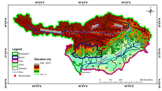
Figure 1.
Catchment boundary of Brahmaputra Basin.
3. Methodology
The methodology used in this research comprised three phases, as shown in Figure 2.
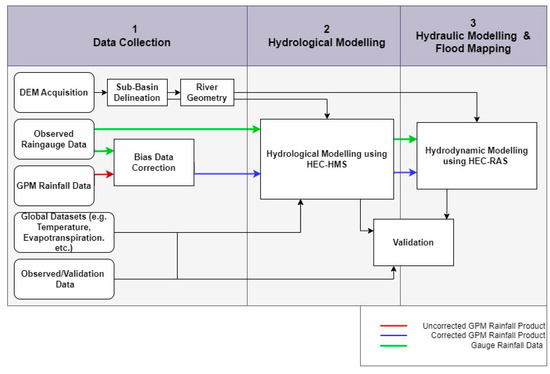
Figure 2.
Flowchart representing the methodology adopted for this research.
3.1. Data Collection and Pre-Processing
In the first step, all the requisite data to be used in the research were collected from all the sources and were pre-processed. For the digital elevation model (DEM), Advanced Spaceborne Thermal Emission and Reflection Radiometer (ASTER) elevation data from NASA and Japanese Space Agency JAXA were used. Tavares et al. [20] carried out research to check the performance of different kinds of freely available DEMs by comparing them with light detection and ranging (LiDAR) data and found that ASTER gave similar elevations to LiDAR. DEM tiles for the expected extent of the basin were downloaded with the coordinates of the southwest vertex of the bounding rectangle as 81°E, 22°N and those of the northeast as 100°E, 33°N. The ASTER tiles were processed in the GIS environment using ArcGIS, based on catchment delineation and using Bahadurabad as the outlet. The whole catchment was divided into 27 sub-basins during the delineation process that was used to develop the semi-distributed hydrological model of the basin.
Monthly average air temperature data from 2 m above ground (NLDAS_FORA0125_M) were required for snowmelt processing in the hydrological model, and were collected from the NASA GIOVANNI website (http://giovanni.sci.gsfc.nasa.gov/giovanni, accessed on 15 December 2020). Monthly average data of evapotranspiration with spatial resolution of 5 arc minutes were acquired from the FAO portal (http://geonetwork.fao.org, accessed on 15 December 2020) for all twelve months. Area average values for all the sub-basins were generated and used. Soil type data were acquired from the Harmonized World Soil Database (HWSD v1.2), which contains indices for every soil type in the named soil mapping unit (SMU), corresponding to which data related to that particular soil were retrieved from HWSD v1.2. To obtain the SMU for every sub-basin, 1 × 1 km raster data were downloaded from the FAO server (http://www.fao.org/soils-portal/data-hub/soil-maps-anddatabases/, accessed on 15 December 2020) and was processed in ArcMap. The zonal statistics tool in ArcGIS was used to assign SMU to each sub-basin through selecting the statistics category as the majority. European Space Agency (ESA) land use/land cover data from Globecover 2009 V2.3 were used in this research; the Globecover map contains the land cover data of the entire earth with a spatial resolution of 300 × 300 m. Lithographic or lithology data were also used in this research, dealing with the underground soil/rock layers and their physical research. These data were used mainly because groundwater movement and storage depend on the hydrogeology (porosity and permeability) of the underground strata [21]. The dataset was acquired from a free data source named Global Lithological Map (GLIM), from the University of Hamburg, Germany [22]. All the datasets used for this research and their respective resolutions are summarized in Table 1.

Table 1.
Summary of datasets used in this research.
For precipitation data, IMERG Early, IMERG Late, and GSMaP-NRT were selected due to their high spatial resolution of 0.1° × 0.1° and relatively short latency period. Resolution and coverage of all three selected SPPs are described in Table 2.

Table 2.
SPPs with their characteristics.
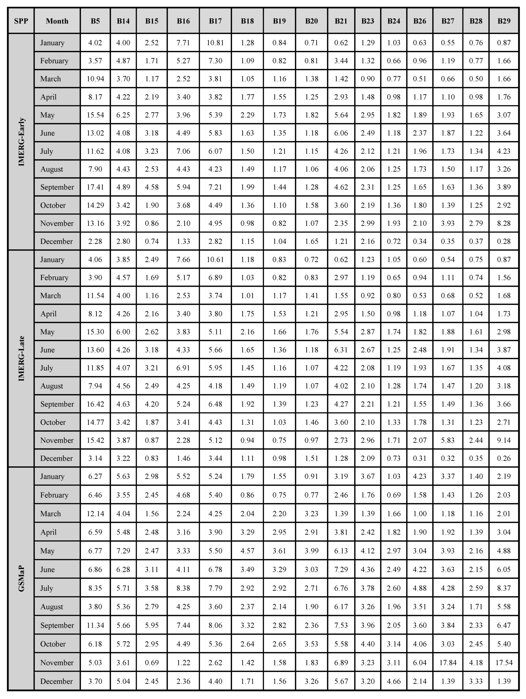
Half-hourly data was downloaded and then aggregated to daily data and averaged for each sub-basin for use in HEC-HMS. In order to use the precipitation data in the hydrological model simulation it was necessary to correct the GPM-based precipitation data for all three selected products, and these were corrected with IMD data (https://mausam.imd.gov.in/responsive/rainfallinformation_swd.php, accessed on 15 December 2020). About 37% of total basin area of Brahmaputra lies in India, for which IMD data were available and were used for data correction, known as bias correction. There are various methods for bias correction of rainfall data, but ratio bias correction (RBC) and quantile mapping (QM) are two potential methods which are more frequently used [23]. In this research, the RBC method was used to find monthly correction factors (four-yearly average, 2013–2016) for all calendar months and for all three selected GPM SPPs, using the RBC equation (Equation (1)):
where CF is the correction factor, GP is gauge precipitation, SPP is satellite precipitation product data, n is number of days in the respective month, k is month number, i is day number (1, 2, 3, … n), and j is sub-basin number (1, 2, … 27). Monthly average ratios for each catchment for each SPP were calculated using RBC for the period of calibration. Once calculated, these ratios were kept fixed and were used for each catchment for a particular SPP (Appendix A). Similarly, the performance of precipitation products was evaluated using the statistical performance indicators mentioned in Table 3. When all three SPPs were compared, based on Table 3, it was found that IMERG-Late outperformed its other two counterparts. GSMaP was found to be the least accurate.

Table 3.
Performance indicators for GPM SPPs.
Considering all three GPM SPPs after correction with IMD data, six sets of precipitation data (Table 4) were prepared and used in the hydrological model.

Table 4.
Different combinations of precipitation datasets.
3.2. Hydrological Model Development
Hydrological modelling of the Brahmaputra Basin was very challenging due to its catchment size and high variability in topography, land use, land cover, altitude, and other hydrometeorology parameters. In this research, a semi-distributed hydrological model of the basin was developed using HEC-HMS modelling software version 4.8 (http://www.hec.usace.army.mil/software/hec-hms/, accessed on 15 December 2020). Pre-processing was carried out in the GIS environment and was exported to the HEC-HMS modelling environment for model development. Specific methods used in this research to model the hydrological processes in the catchment are listed in Table 5.

Table 5.
Summary of methods used for hydrological model components.
The model was provided with the initial values for its different components. For the canopy component, maximum storage capacity of all sub-basins varied from 1 to 7 mm based on the vegetation/forest cover percentage. A value of 1mm was chosen for barren basins, which are mostly in the upstream parts of the basin. The initial values for canopy storage were set to 0 mm as initial values do not affect model results after simulation over a few months [6]. For surface storage in depressions, upper threshold values were set between 6 and 10 mm based on the topography of sub-basins, whereas initial values were set as zero. To model direct runoff in the form of excess rainfall, Clark unit hydrography (CUH) was used, which required certain inputs. The lag time was calculated based on the longest flow path, based on which the time of concentration was computed, which ranged between 50 and 131 h. The other input was storage coefficient, which was set between 5 and 12 h based on the size of each sub-basin. Meteorological input methods selected for evapotranspiration and snowmelt for the HMS model development were monthly average evapotranspiration (ET) and temperature index method, respectively. The monthly average ET values were acquired from FAO and the daily average temperature data was taken from NASA (http://giovanni.sci.gsfc.nasa.gov/giovanni, accessed on 15 December 2020). After the initial setting up of the model, it was necessary to divide the total modelling timeline into two parts for calibration of model parameters and then for validation of the model output, which is described in Table 6.

Table 6.
Hydrological model calibration and validation periods.
The method used for calibration was the univariate gradient search algorithm, which is an automatic calibration method available in HEC-HMS. As there were six different SPPs, the model was calibrated six times considering a different SPP each time. This resulted in six sets of calibrated parameter values. The parameters that were considered in the optimization process were storage coefficient and time of concentration from CUH, groundwater storage coefficients GW1 and GW2 for the linear reservoir baseflow model, and soil storage, soil percolation rate, and groundwater storage coefficient GW1 for the soil moisture accounting (SMA) loss model. Note that HMS allows consideration of two layers of groundwater. For the maximum infiltration rate, which is also a parameter of SMA, a scale factor for all the sub-basins ranging between 1 and 100 was considered. This was carried out to minimize the number of parameters to be determined during the optimization. The obtained scale factor was used to multiply the initially estimated values of maximum infiltration rate to determine the optimized values of maximum infiltration rate for all the sub-basins. Therefore, all the above-mentioned parameters were optimized and used for further simulations, with the simulation time step of 1 day. The performance of the model-generated results was evaluated during calibration and validation by calculating the statistical parameters listed in Table 3.
3.3. Hydraulic Model Development
The hydraulic model was developed for the last 500 km of the Brahmaputra River and was used to evaluate the performance of the SPPs in flood inundation mapping. The hydraulic model used the discharge values simulated by the hydrological model. The floodplain areas adjacent to the selected river reach were more prone to flooding. The observed flow data were available from Bahadurabad station, and were used for the calibration of the model. Pre-processing of the model was carried out in ArcGIS where cross-sections, bank lines, river stream lines, and flow direction were defined. Elevation values were extracted from ASTER DEM for all the cross-sections because actual bathymetry data of the riverbed and in situ elevation data of the flood plain were missing. Bhattacharya et al. [6] used Shuttle Radar Topography Mission (SRTM) elevation data for flood inundation mapping of the Brahmaputra Basin and found this approach useful in developing a hydraulic model and for flood extent mapping. The geographical information in ArcGIS was exported to HEC-RAS where final processing regarding model development was carried out. The upstream boundary condition for the hydraulic model was the discharge data simulated using HEC-HMS and the downstream boundary condition was taken as the normal depth of the selected river channel. The model was calibrated using the gauge data from Bahadurabad station from 1 January 2015 to 31 December 2015. Validation was carried out for the year 2017 via comparing the simulated river stage values with the measured stage values at Bahadurabad and Tezpur. The hydraulic model was further simulated for the year 2019 and the flood inundation maps were prepared for the seven areas shown in Figure 3.
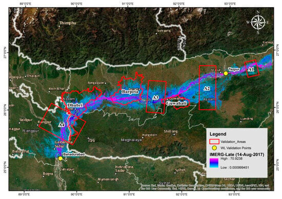
Figure 3.
Location of areas for flood extent validation of the hydraulic model.
In the absence of measured discharge data inside the model domain, validation of the hydraulic model was an issue. Satellite altimetry data from different sources such as CryoSat-2, ENVISAT, and Jason2 (now Jason3) can provide estimates of water level data. In this regard, various researchers have used altimetry data to predict discharge. For example, Papa et al. [24] used satellite altimetry data from ERS-2, TOPEX-Poseidon, and ENVISAT for predicting monthly flow for Ganges–Brahmaputra with an accuracy of about 15–20%. Similarly, Schneider et al. [25] used CryoSat-2 altimetry data for the calibration of cross-sectional data of the Brahmaputra River and found good results.
In this research, Jason2 altimetry data (from NASA) were used, which were available from Hydroweb of Thiea Land Data Services for the virtual gauging stations at Tezpur and Bahadurabad. Similarly, for flood extent validation, digitized images of two selected flooding events (14 August 2017 and 16 July 2019) were acquired from Dartmouth Flood Observatory (DFO) of Colorado University, USA (https://floodobservatory.colorado.edu/FloodMapIndex.htm, accessed on 15 December 2020), which has the largest digitized database of floods in the world since 2011. The data were available in binary raster form and were processed in ArcMap for further computation.
Each of the flood inundation maps simulated via the hydraulic model for the two above-mentioned flood events were converted to binary maps so that any pixel (30 × 30 m) having a flood depth greater than a threshold was considered as 2 (wet pixel) or 1 (dry pixel) otherwise. The DFO rasters for the corresponding two flood events were also converted to binary rasters: 2 (wet pixel) and 1 (dry pixel). Note that there was no information about flood depth in the DFO raster (or any satellite-observed flood inundation map). In satellite-observed flood images, identifying wet pixels for very low flood depths is an issue [6]. In order to minimize this problem, a threshold of 0.1 m was used in converting the simulated inundation map to the binary raster. This means that if the simulated depth for a pixel was >0.1 m, then that pixel was assigned a value of 2 or otherwise, 1. For each flood event, the binary map from the simulated inundation map and the DFO raster were added and subtracted from each other one by one. The two resultant rasters for each of the flooding events had one of four possible values for each pixel (Table 7).

Table 7.
Classification of pixel values.
Correct alarms and positive rejections were extracted from the added rasters, while false and missed alarms were extracted from the subtraction of rasters. In the last step, unified maps were generated that contained all four types of output combinations. The unified maps (new_raster) were generated using the raster calculator in ArcGIS, applying the following conditional:
If subtracted_raster_value = 0:
New_raster_value = added_raster_value
Else:
New_raster_value = subtracted_raster_value
The above expression merged all the four types of pixel values into one new raster which contains all the four classes. Model performance in the selected administrative and regional areas was evaluated using the following indices: probability of detection (POD), false alarm ratio (FAR), success ratio (1-FAR), and critical success index (CSI).
where C = correct alarms (correct alarms and positive rejections), F = false alarms, and M = missed alarms.
4. Results and Discussion
4.1. Hydrological Model Results
The results from different model runs are shown in Figure 4.
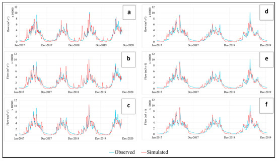
Figure 4.
Validation hydrograph generated with (a) dataset 1, showing that low flows were not predicted well, but high flows showed a good match with observed flows; (b) 2, performed very similarly, a with a small improvement in low flows; (c) 3, both high and low flows visually performed close to observed flows; (d) 4, with addition of IMD data, the low flow overestimation problem of case a was resolved considerably; (e) 5, performed very similarly to case d with a small improvement; and (f) 6, both high and low flows were predicted well by the model.
All the simulation runs indicated that the simulated discharge followed the trend of the observed discharge. However, low flows were overpredicted by the model, especially when GPM data was used for the Indian part; however, this model trend improved somewhat with the introduction of IMD data for the Indian part of the catchment. The statistical performance of the model is shown in Table 8. It can be observed that all the model runs gave good values of NSE and R2. Moreover, for the first three datasets (1, 2, 3), NSE and R2 values were in the range of 0.70 to 0.80, which increased for the last three datasets when IMD data were used for the Indian part of the basin. IMERG-Late performed better than IMERG-Early and GSMaP and showed higher values of NSE and R2. Therefore, the performance of the model was improved for IMERG-Late when the IMD data was used for the Indian part of the basin (Dataset 5), thereby increasing the NSE from 0.773 to 0.844 and reducing RMSE from 7711 m3 s−1 to 7125 m3 s−1, whereas the average observed flow for the validation period was 20,611 m3 s−1. It is pertinent to mention that although the results improved when IMD data were used for the Indian part of the basin, the datasets without IMD data still performed very well in hydrological modelling, with high model indicators as shown in Table 8.

Table 8.
Hydrological model performance indicators in validation.
The same was the case for all the other datasets because their performance also improved when IMD precipitation data were used for the Indian part of the basin. The performance of different precipitation datasets in hydrological modelling can also be represented using Taylor’s diagram (Figure 5), which is a mathematical diagram used to show which model results perform better in comparison with others.
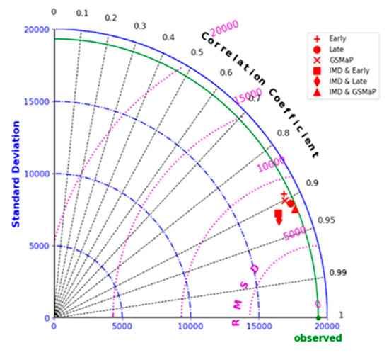
Figure 5.
Taylor diagram for model performance in validation.
The figure shows standard deviation, RMSE, and coefficient of correlation (CC) in one plot, from which is convenient to understand which model outputs were better than others. It can be observed that out of all six datasets, IMD-Late outperformed all of its counterpart SPPs tested in this research, having minimum RMSE and the highest CC. The point represented as observed is the reference point which shows the statistics of the observed flow. The simulation result that was closest to the reference point was regarded as the best model result, which in this case was IMD-Late. Similarly, all the model runs had RMSE between 5000 and 10,000 m3 s−1 with CC values ranging between 0.85 and 0.95. The same was the case with all the other datasets, because their performance also improved when IMD precipitation data were used for the Indian part of the basin. Bhattacharya et al. [6] tested TMPA 3B42 for the Brahmaputra Basin and found that it was useful in hydrological modelling with NSE in the range of 0.7 and 0.75 for corrected precipitation datasets. Uncertainty in boundary flow data by Ahmed et al. [16] using TMPA and GPM over a medium size basin in South Asia. Peng et al. [15] used IMERG and GSMaP for a small basin in Central Asia and confirmed the useability of remotely sensed datasets for data-scarce basins. However, the results of this study highlight its usability for large and trans-boundary basins and further strengthen the argument that with use of GPM products, performance in hydrological modelling can be improved.
4.2. Hydraulic Model Results
The 1D hydraulic model (discussed in Section 3.3) was simulated using the discharge values generated by the hydrological model using all six precipitation datasets. The simulated water levels at Bahadurabad station were plotted along with Jason2 satellite altimetry water levels for the same period. The comparison is shown here with six chosen precipitation datasets (Figure 6).

Figure 6.
Validation of hydraulic model (WL) at Bahadurabad.
The difference between simulated and observed values was larger when the water level was increasing (due to increasing flows) compared with when the water in the river was receding. The statistical model performance is illustrated in Table 9. Water extent rasters were generated from the hydraulic model, based on different SPPs. Raster maps containing four cell types including correct alarms (hits), missed alarms (misses), false alarms, and positive rejections, as explained in Section 3.3, were developed for both the flooding events (14 August 2017 and 16 July 2019). Hits, misses, and false alarms with IMREG-Late for both the flooding events are shown in Figure 7.

Table 9.
Hydraulic model performance in validation of water level.
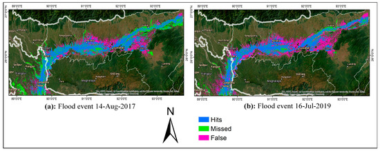
Figure 7.
Accuracy of the simulated inundation maps based on IMERG-Late precipitation dataset against corresponding DFO rasters.
It can be observed in Figure 7 that there seems to be a good agreement between the simulated and observed flood extent, particularly in the lower part of the hydraulic model domain (downstream of Barpeta). At the upstream section, the model showed over-prediction (a large number of false alarms). False alarms may be generated if the digital elevation model used does not include any existing embankment or other protection measures. This may have originated from the coarser resolution of the ASTER GDEM digital elevation data. Similarly, linear interpolation of the cross section in HEC-RAS could be another reason for error in the results predicted by the model. Other sources of errors could be in the DFO flood rasters. Satellite imageries, such as from Landsat, were used in a binary classification algorithm to determine class of each pixel as land or water. These classification algorithms tend to be erroneous for low water depths and for water areas bordering land [26]. Uncertainty in boundary flow data could also be another major error source. However, POD, SR, and CSI values were computed for all the selected areas for validation of flood extent to check the performance of SPPs in hydraulic modelling for flood inundation mapping. It was noticed that for all the SPPs, CSI, POD, and SR values were more than ~0.7, which represents a good model result. Figure 8 shows the POD, SR, and CSI of different outputs of the hydraulic model for the flooding events of 14 August 2017 and 16 July 2019.
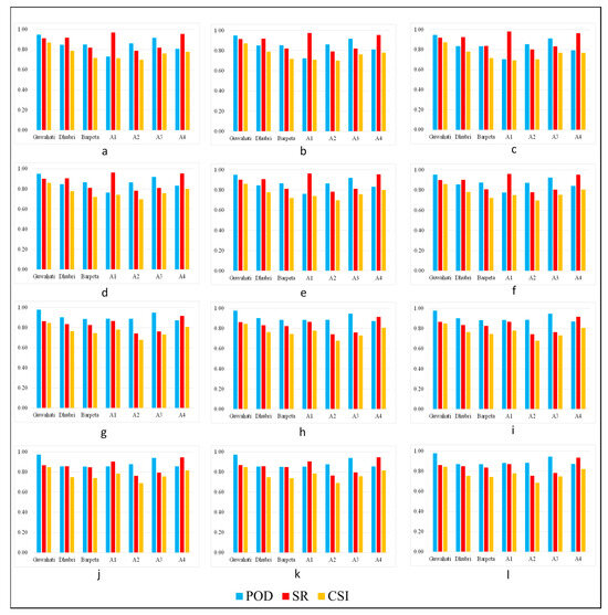
Figure 8.
Performance indicators of the hydraulic model for the flood event on 14 August 2017 with SPP (a) 1, (b) 2, (c) 3, (d) 4, (e) 5, (f) 6 and for the flood event on 16 July 2019 with SPP (g) 1, (h) 2, (i) 3, (j) 4, (k) 5, (l) 6.
Despite good results in hydrological and hydraulic modelling, there are certain limitations associated with this study. Calibration of the hydrological model was carried out for only 2.5 years, and calibration was conducted only using one location (catchment outlet) because of the limited data availability. Similarly, uncertainties in the datasets used were another source of uncertainty in the results. Also, there are limitations regarding channel bed elevation estimation for hydraulic modelling and there is a need for further investigations.
5. Conclusions
Based on the results of this study, the following conclusions are drawn:
- (i)
- All three near real-time SPPs (IMERG-Early, IMERG-Late, and GSMaP) performed very well in the development of the hydrological model of the sparsely gauged Brahmaputra Basin. The general trend of the observed flow hydrograph at the catchment outlet was followed very well by the simulated hydrographs for all three SPPs, particularly for high flows. Low flows were not predicted well by the model; however, the trend of the simulated hydrograph was comparable to the observed one. Performance indicators for the hydrological model simulation in calibration and validation showed adequately good values for NSE (above 0.73), R2 (above 0.77) for all the SPPs, and maximum RMSE of 9120 m3 s−1 (where the average observed flow was 20,611 m3 s−1).
- (ii)
- Although all the near real-time GPM-era SPPs performed well when used for the development of the hydrological model of a sparsely gauged large catchment, there were some performance differences. IMERG-Early and IMERG-Late performed very similarly to each other as the difference between these two products is mainly in the retrieving algorithm, but still, the performance of IMERG-Late was slightly better than IMERG-Early. Both IMERG products outperformed GSMaP, because hydrological simulations with GSMaP as input over-estimated medium and small peak flows. Based on the performance indicators, it can be concluded that IMERG-Late performed better than IMERG-Early and GSMaP and hence should be prioritized when selecting GPM-era SPPs.
- (iii)
- The performance of the hydrological model was improved when IMD station precipitation data were used (37% of the basin area). Flow hydrograph trends were improved, even in cases of low flows. Similarly, performance indicators also improved, with NSE values increasing to 0.844 when IMD-Late (dataset 5, Table 4) was used, which was 0.773 when IMERG-Late (dataset 2, Table 4) was used. Moreover, RMSE reduced to 7125 m3 s−1 from 7711 m3 s−1 (where the average observed flow was 2061 m3 s−1).The performance indicators of the model were found to be better than those for the TMPA 3B42 precipitation-based hydrological model of Brahmaputra reported by Bhattacharya et al. [6], although they were tested for a different time period. This gives an indication that near real-time GPM precipitation datasets perform better than TRMM based datasets in hydrological modelling of large catchments. For the case of the Brahmaputra Basin, it can be concluded that although the results improved when IMD observed data were used for the Indian part of the basin, the datasets without IMD data still performed very well in hydrological modelling, with high performance indicator scores as shown in Table 8.
- (iv)
- For the 1D hydraulic model simulation results, it was found that with all the GPM-based upstream boundary flow datasets, R2 values for the simulated water level at Bahadurabad gauging station, compared with Jason2 altimetry data, were above 0.6, and at Tezpur, the R2 values were above 0.43. The general trend of Jason2 data was followed by the simulated water level in all the hydraulic model simulations based on GPM-generated boundary flow datasets. Although there were differences in some parts of the simulated water levels in comparison with Jason2, particularly at the start of the rainy season, the error was limited within a range of 0.5 to 1.5 m.
- (v)
- Validation of the flood inundation maps revealed that the simulated flood extent matched well with the observed one. In the upstream part of the model domain up to Tezpur, the inundation cells showed a relatively higher percentage of false alarms and missed events for both floods (14 August 2017 and 16 July 2019). The POD and CSI indicators showed that the model performance in flood inundation was reasonably good. The POD and CSI values for all the model runs were above 0.70 for all the validation areas in both of the flood events. It is noteworthy that the model performance was approximately same for all three GPM-based boundary flow datasets. So, for the purpose of flood inundation mapping, any of the near-real time GPM SPPs tested, IMERG-Early, IMERG-Late, and GSMaP, can be used.
Overall, the performance of the hydrological and hydrodynamic model simulations of the Brahmaputra Basin showed the potential of using near real-time GPM satellite precipitation products for discharge simulation and flood inundation mapping in sparsely gauged large catchments.
Author Contributions
Conceptualization, B.B.; Methodology, M.J.; Formal analysis, M.J.; Writing—original draft, M.J.; Writing—review & editing, B.B., A.Y. and S.J.v.A.; Supervision, B.B., A.Y. and S.J.v.A. All authors have read and agreed to the published version of the manuscript.
Funding
This research received no external funding.
Data Availability Statement
All the data used in this study as publicly available online except IMD rainfall data which cannot be shared due to data sharing restrictions.
Conflicts of Interest
The contact author has declared that none of the authors have any competing interests.
Appendix A
References
- Xiang, Y.; Chen, J.; Li, L.; Peng, T.; Yin, Z. Evaluation of eight global precipitation datasets in hydrological modeling. Remote Sens. 2021, 13, 2831. [Google Scholar] [CrossRef]
- Su, F.; Hong, Y.; Lettenmaier, D.P. Evaluation of TRMM Multisatellite Precipitation Analysis (TMPA) and its utility in hydrologic prediction in the La Plata Basin. J. Hydrometeorol. 2008, 9, 622–640. [Google Scholar] [CrossRef]
- Li, X.-H.; Zhang, Q.; Xu, C.-Y. Suitability of the TRMM satellite rainfalls in driving a distributed hydrological model for water balance computations in Xinjiang catchment, Poyang Lake basin. J. Hydrol. 2012, 426, 28–38. [Google Scholar] [CrossRef]
- Ochoa, A.; Pineda, L.; Crespo, P.; Willems, P. Evaluation of TRMM 3B42 precipitation estimates and WRF retrospective precipitation simulation over the Pacific–Andean region of Ecuador and Peru. Hydrol. Earth Syst. Sci. 2014, 18, 3179–3193. [Google Scholar] [CrossRef]
- Meng, J.; Li, L.; Hao, Z.; Wang, J.; Shao, Q. Suitability of TRMM satellite rainfall in driving a distributed hydrological model in the source region of Yellow River. J. Hydrol. 2014, 509, 320–332. [Google Scholar] [CrossRef]
- Bhattacharya, B.; Mazzoleni, M.; Ugay, R. Flood inundation mapping of the sparsely gauged large-scale Brahmaputra basin using remote sensing products. Remote Sens. 2019, 11, 501. [Google Scholar] [CrossRef]
- Thiemig, V.; Rojas, R.; Zambrano-Bigiarini, M.; De Roo, A. Hydrological evaluation of satellite-based rainfall estimates over the Volta and Baro-Akobo Basin. J. Hydrol. 2013, 499, 324–338. [Google Scholar] [CrossRef]
- Bitew, M.M.; Gebremichael, M. Evaluation of satellite rainfall products through hydrologic simulation in a fully distributed hydrologic model. Water Resour. Res. 2011, 47. [Google Scholar] [CrossRef]
- Tian, Y.; Peters-Lidard, C.D. A global map of uncertainties in satellite-based precipitation measurements. Geophys. Res. Lett. 2010, 37, L24407. [Google Scholar] [CrossRef]
- Huffman, G.; Bolvin, D.; Braithwaite, D.; Hsu, K.; Joyce, R.; Xie, P. Integrated Multi-satellitE Retrievals for GPM (IMERG), version 4.4. NASA’s Precipitation Processing Center. 2014. Available online: ftp://arthurhou.pps.eosdis.nasa.gov/gpmdata (accessed on 1 October 2020).
- Foelsche, U.; Kirchengast, G.; Fuchsberger, J.; Tan, J.; Petersen, W.A. Evaluation of GPM IMERG Early, Late, and Final rainfall estimates using WegenerNet gauge data in southeastern Austria. Hydrol. Earth Syst. Sci. 2017, 21, 6559–6572. [Google Scholar] [CrossRef]
- Gaona, M.R.; Overeem, A.; Leijnse, H.; Uijlenhoet, R. First-year evaluation of GPM rainfall over the Netherlands: IMERG day 1 final run (V03D). J. Hydrometeorol. 2016, 17, 2799–2814. [Google Scholar] [CrossRef]
- Kim, K.; Park, J.; Baik, J.; Choi, M. Evaluation of topographical and seasonal feature using GPM IMERG and TRMM 3B42 over Far-East Asia. Atmos. Res. 2017, 187, 95–105. [Google Scholar] [CrossRef]
- Tang, G.; Ma, Y.; Long, D.; Zhong, L.; Hong, Y. Evaluation of GPM Day-1 IMERG and TMPA Version-7 legacy products over Mainland China at multiple spatiotemporal scales. J. Hydrol. 2016, 533, 152–167. [Google Scholar] [CrossRef]
- Peng, J.; Liu, T.; Huang, Y.; Ling, Y.; Li, Z.; Bao, A.; Chen, X.; Kurban, A.; De Maeyer, P. Satellite-based precipitation datasets evaluation using gauge observation and hydrological modeling in a typical arid land watershed of Central Asia. Remote Sens. 2021, 13, 221. [Google Scholar] [CrossRef]
- Ahmed, E.; Al Janabi, F.; Zhang, J.; Yang, W.; Saddique, N.; Krebs, P. Hydrologic assessment of TRMM and GPM-based precipitation products in transboundary river catchment (Chenab River, Pakistan). Water 2020, 12, 1902. [Google Scholar] [CrossRef]
- Abdessamed, D.; Abderrazak, B. Coupling HEC-RAS and HEC-HMS in rainfall–runoff modeling and evaluating floodplain inundation maps in arid environments: Case study of Ain Sefra city, Ksour Mountain. SW of Algeria. Environ. Earth Sci. 2019, 78, 586. [Google Scholar] [CrossRef]
- Sarma, J. Fluvial process and morphology of the Brahmaputra River in Assam, India. Geomorphol. 2005, 70, 226–256. [Google Scholar] [CrossRef]
- Parua, P.K. The Ganga: Water Use in the Indian Subcontinent; Springer Science & Business Media: Berlin/Heidelberg, Germany, 2010. [Google Scholar]
- Tavares da Costa, R.; Mazzoli, P.; Bagli, S. Limitations posed by free DEMs in watershed studies: The case of river Tanaro in Italy. Front. Earth Sci. 2019, 7, 141. [Google Scholar] [CrossRef]
- Bell, F.; Cripps, J.; Culshaw, M. A review of the engineering behaviour of soils and rocks with respect to groundwater. Geol. Soc. Lond. Eng. Geol. Spec. Publ. 1986, 3, 1–23. [Google Scholar] [CrossRef]
- Hartmann, J.; Moosdorf, N. The new global lithological map database GLiM: A representation of rock properties at the Earth surface. Geochem. Geophys. Geosystems 2012, 13. [Google Scholar] [CrossRef]
- Mastrantonas, N.; Bhattacharya, B.; Shibuo, Y.; Rasmy, M.; Espinoza-Dávalos, G.; Solomatine, D. Evaluating the benefits of merging near-real-time satellite precipitation products: A case study in the Kinu basin region, Japan. J. Hydrometeorol. 2019, 20, 1213–1233. [Google Scholar] [CrossRef]
- Papa, F.; Bala, S.K.; Pandey, R.K.; Durand, F.; Gopalakrishna, V.V.; Rahman, A.; Rossow, W.B. Ganga-Brahmaputra river discharge from Jason-2 radar altimetry: An update to the long-term satellite-derived estimates of continental freshwater forcing flux into the Bay of Bengal. J. Geophys. Res. Ocean. 2012, 117. [Google Scholar] [CrossRef]
- Schneider, R.; Godiksen, P.N.; Villadsen, H.; Madsen, H.; Bauer-Gottwein, P. Application of CryoSat-2 altimetry data for river analysis and modelling. Hydrology and Earth System Sciences 2017, 21, 751–764. [Google Scholar] [CrossRef]
- Mueller, N.; Lewis, A.; Roberts, D.; Ring, S.; Melrose, R.; Sixsmith, J.; Lymburner, L.; McIntyre, A.; Tan, P.; Curnow, S.; et al. Water observations from space: Mapping surface water from 25 years of Landsat imagery across Australia. Remote Sens. Environ. 2016, 174, 341–352. [Google Scholar] [CrossRef]
Disclaimer/Publisher’s Note: The statements, opinions and data contained in all publications are solely those of the individual author(s) and contributor(s) and not of MDPI and/or the editor(s). MDPI and/or the editor(s) disclaim responsibility for any injury to people or property resulting from any ideas, methods, instructions or products referred to in the content. |
© 2024 by the authors. Licensee MDPI, Basel, Switzerland. This article is an open access article distributed under the terms and conditions of the Creative Commons Attribution (CC BY) license (https://creativecommons.org/licenses/by/4.0/).