Abstract
The sea surface temperature (SST) is one of the most important parameters that characterize the thermal state of the ocean surface, directly affecting the heat exchange between the ocean and the atmosphere, climate change, and weather generation. Generally, due to factors such as the weather, satellite scanning orbit range, and satellite sensor malfunction, there are large areas of missing satellite remote sensing SST data, greatly reducing data utilization. In this situation, how to use effective data or avenues to rebuild missing SST data has become a research hotspot in the field of ocean remote sensing. Based on the SST data from an FY-3C visible and infrared radiometer with a spatial resolution of 5 km (FY-3C VIRR), an improved data interpolation convolutional autoencoder (I-DINCAE) was used to reconstruct the missing SST data. Through cross-validation, the accuracy of the reconstruction results was quantitatively evaluated with an RMSE of 0.36 °C and an MAE of 0.24 °C. The results showed that the I-DINCAE algorithm outperformed the original DINCAE algorithm greatly. For further optimization, a deep neural network (DNN) was chosen to adjust the error between the reconstructed SST and the in situ data. The RMSE of the final adjusted SST and in situ data is 0.466 °C, and the MAE is 0.296 °C. Compared to the in situ data, the accuracy of the adjusted data has shown a significant improvement over the reconstructed data. This method successfully applies deep-learning technology to the reconstruction of SST data, achieving the full coverage and high accuracy of SST products, which can provide more reliable and complete SST data for marine scientific research.
1. Introduction
The sea surface temperature (SST) characterizes the thermal conditions of the upper layer of the ocean and plays an important role in oceanography and meteorology [1,2,3]. Additionally, it is highly sensitive to atmospheric circulation and short-term climate variations, making it a vital component in monitoring climate events such as typhoons and El Niño, including their occurrence and development [4]. Therefore, accurately obtaining SST information is essential for the development and utilization of ocean resources and the study of various phenomena in the ocean.
Currently, ocean temperature data from diverse sources such as Argo floats, oceanic vessels, and observation platforms are steadily increasing. However, the limited coverage of in situ ocean observation data poses challenges related to the non-uniform spatial distribution and discrete temporal patterns, resulting in the difficulty in acquiring large-scale synchronized SST data [5,6,7]. In contrast to traditional SST monitoring methods, remote sensing technology has the characteristics of having a large scale, wide coverage, and strong continuity, which can cover a wide range of ocean regions and provide global ocean data. The real-time monitoring of satellite data enhances the timeliness and accuracy of oceanic information surveillance and forecasting. Satellite remote sensing technology can better compensate for the limitations of traditional methods, making it an effective way to obtain SST data. Nevertheless, factors such as the atmospheric conditions, sensor quality, satellite scan width, and revisit period contribute to varying degrees of missing data issues. Therefore, effective methods are needed to reconstruct missing information to obtain complete remote sensing images, which is of great significance for monitoring and studying the marine ecological environment.
Common methods for reconstructing missing data include interpolation, statistical modeling, machine-learning-based, and deep-learning-based methods. Interpolation methods based on adjacent pixels, such as nearest-neighbor interpolation, bilinear interpolation, bicubic interpolation, etc., use the information of surrounding pixels to estimate missing pixels and achieve spatial interpolation [8]. Spatial interpolation methods based on statistical modeling are suitable for remote sensing data with spatial autocorrelation, such as Optimal Interpolation (OI), Kriging Interpolation, and Data Interpolation Empirical Orthogonal Function (DINEOF). The optimal interpolation method was initially proposed by Eliassen in 1954, and further developed by Gandin based on the stepwise correction method [9]. Based on the contribution of surrounding points to the interpolation points, the interpolation weights of each known point were calculated using specific mathematical methods in the optimal interpolation method. Reynolds and Smith applied the optimal interpolation method to analyze the global sea surface temperature [10]. In addition, Everson et al. also applied the idea of optimal interpolation to reconstruct and analyze the sea surface temperature in the western North Atlantic; Kriging interpolation, also known as spatial auto-correlation best interpolation, is a common geostatistical method that can interpolate existing sample data and predict missing parts of the data. Müller filled the MERIS ocean chlorophyll concentration image using the Kriging method [11]. Feng et al. used the Kriging interpolation method to restore pixel information in the cloud-shadow-obscured areas of the image. The restored information was further classified and compared with the results of the two-class resource survey. The findings indicated a classification accuracy of over 75%, suggesting that kriging interpolation provides a method for interpreting ambiguous areas in the image [12]. Yu et al. utilized the geostatistical Kriging spatial interpolation method to interpolate missing data in the monthly averaged remote sensing images of the sea surface chlorophyll-a concentration. The results indicated that the interpolation with the Kriging method could reflect the spatiotemporal variation patterns of the chlorophyll-a concentration in marine areas. The root means square error (RMSE) of the reconstruction results averaged 0.46, with an average standardized RMSE of 2.61 [13]. The DINEOF method is based on the principles of empirical orthogonal function (EOF) and data interpolation, aiming to remove noise and fill in missing values from the observation dataset, thereby obtaining a more complete and smoother spatial and temporal scene [14,15,16,17,18,19,20]. Sheng et al. successfully reconstructed the SST data in the Yangtze River Estuary and parts of the South China Sea using the DINEOF algorithm, achieving a reconstruction accuracy of 0.94 °C. Furthermore, the effectiveness of DINEOF was tested using data from the South China Sea, with a reconstruction accuracy of 0.81 °C [21]. Due to the use of spatial correlation to estimate interpolation, these methods are simple and easy to use but have strict assumptions about the distribution of data, which may make it difficult to effectively capture the complex relationships of data. Machine-learning methods can automatically analyze data and use patterns to predict unknown data in a supervised or unsupervised manner. Artificial neural networks (ANN), support vector machines (SVM), and random forests (RF) are some common machine-learning methods. Jouini M et al. used an artificial neural network self-organizing mapping (SOM) algorithm to reconstruct missing values in satellite chlorophyll-a concentration product data in the western North Atlantic region. They used sea surface temperature SST and altitude (SSH) data as predictive factors for CHL estimation. The results showed that in the presence of thick clouds, SOM reconstruction of chlorophyll-a data was also reliable at scales greater than 10 km [22]. Park et al. used an ensemble machine-learning method based on random forests to reconstruct chlorophyll in the Ross Sea, and the results showed that the reconstructed CHL data was consistent with satellite measurements [23]. However, machine-learning models are relatively shallow and have limited processing capabilities for highly complex non-linear features. With the advancement of artificial intelligence technology, deep-learning methods have demonstrated outstanding performance in reconstructing missing data. For example, techniques such as Convolutional Neural Networks (CNNs) and Recurrent Neural Networks (RNNs) have been widely employed for the spatial reconstruction of satellite remote sensing data, yielding reliable results in terms of accuracy and computational efficiency. These methods introduce non-linear transformations, enabling the effective capturing of complex spatial distributions and temporal dependencies in the data, thus better learning from the data and predicting intricate trends, making them emerging solutions for data reconstruction. Krasnopolsky et al. employed neural network technology (NN) to reconstruct ocean color data globally based on physical variables measured by satellites (such as SST, SSH, SSS, and in situ Argo data). This method offers an accurate and cost-effective approach to fill in the gaps in satellite observations [24].
The Data Interpolation Convolutional Autoencoder (DINCAE) proposed by Barth et al. adopts an OI-based convolutional autoencoder structure [25]. Unlike traditional linear-assumption-based OI methods, DINCAE endows OI with non-linear interpretability through a series of convolutional operations. DINCAE has successfully addressed the limitations of DINEOF in handling non-linear relationships in time and space domains. By fully utilizing the powerful capabilities of neural networks, DINCAE can effectively handle complex interactions and non-linear relationships. Li et al. proposed the T-DINCAE method based on the original DINCAE, incorporating Convolutional LSTM (ConvLSTM) to enhance the extraction of temporal features from data. They applied both DINCAE and T-DINCAE methods to reconstruct sea surface temperature data from MODIS in the South China Sea for the period 2002–2022. Through cross-validation and comparison with Argo buoy data, the results demon-strated that the T-DINCAE method achieves superior reconstruction performance [26]. Xiong used the DINCAE method to reconstruct chlorophyll-a concentration data in the South China Sea and compared it with DINEOF. They evaluated the reconstruction ability of these two methods using cross-validation data. The reconstruction error of DINCAE was lower than that of DINEOF, and it was able to retain more small-scale detail features of the original image, confirming the superiority of the DINCAE reconstruction algorithm [27]. Traditional neural network training requires complete datasets, which are often lacking in satellite remote sensing image reconstruction. In contrast, the DINCAE algorithm can utilize missing data for network training, making it widely applicable in satellite remote sensing image reconstruction.
Improving the width and depth of CNNs enhances their performance. However, with an increased depth and width, the parameter counts rise, posing risks of overfitting and escalating the computational complexity. Hence, in this study, an improved DINCAE (I-DINCAE) model was adopted to reconstruct SST data in the South China Sea. The introduction of an Inception module to the DINCAE network augments its generalization and structural expression capabilities via multiple convolutional kernels of various scales, significantly boosting feature learning [28]. This module applies convolutional operations of different scales to input feature maps, progressively expanding the receptive field of the network. Subsequently, the obtained feature maps are connected to better understand the global information and contextual relationships in images. Compared to the original DINCAE, this approach can improve reconstruction accuracy.
The article’s remaining sections are organized as follows: The overview of the South China Sea and the data sources utilized are presented in Section 2. Section 3 provides an in-depth explanation of the methods used in this study, combined with a flowchart to aid in mastering the methodology presented in this paper. Section 4 shows the results and discusses potential directions for further research. Finally, Section 5 presents the conclusions of this study.
2. Study Area and Data
2.1. Study Area
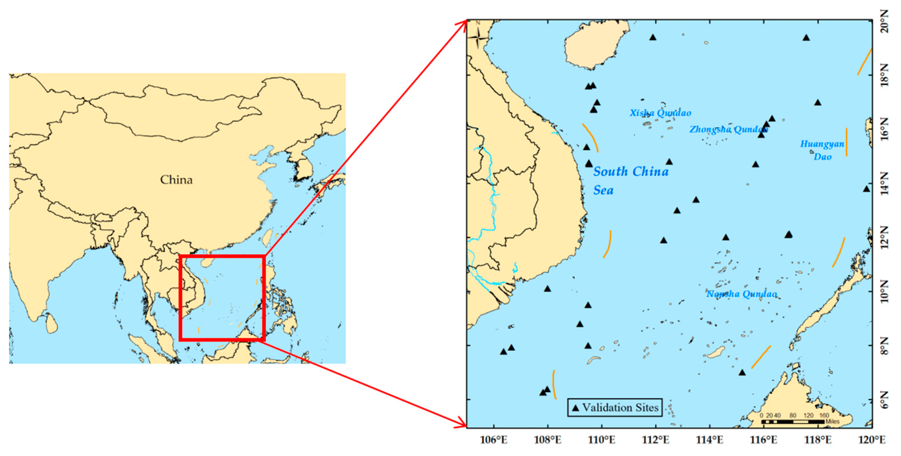
The South China Sea (SCS) and its surrounding waters (5–20°N, 105–120°E) were chosen as the study area (Figure 1). As the largest continental margin sea in the western Pacific, the SCS is primarily influenced by the East Asian monsoon system. It presents a complex and variable circulation structure and is susceptible to various mesoscale oceanic phenomena such as eddies, fronts, and upwelling among others [29]. Precipitation is plentiful in the South China Sea, with consistently high temperatures throughout the year, which shows a typical tropical oceanic monsoon climate. Temperature fluctuations are minimal across the year, ranging from approximately 23 °C to 26 °C in the north, 26 °C to 27 °C in the middle, and 27 °C to 28 °C in the south, with peak temperatures reaching 31 °C to 32 °C. The overall terrain of the SCS is diverse and intricate, characterized by numerous coral reefs and islands. Its climate is monsoonal year-round, with distinct seasonal variations [30]. Given the unique geographical positioning of the SCS, its circulation patterns, and the presence of multi-temporal and spatial atmospheric systems, it has emerged as a pivotal region for studying ocean–atmosphere interactions [31]. To gain a deeper insight into the temporal and spatial fluctuations of these oceanic processes across different scales, a high-resolution and complete SST dataset is deemed essential [32].

Figure 1.
Study area (5–20°N, 105–120°E). The triangles denote the validation sites.
2.2. Satellite and In situ Data
This study used FY-3C infrared data provided by the National Satellite Meteorological Center to acquire Level 2 daily SST products (http://data.nsmc.org.cn/ (accessed on 12 June 2023)). The infrared data employed are Visible and Infrared Radiometer (VIRR) SST, featuring a spatial resolution of 0.05° × 0.05° and a temporal resolution of 1 day. It is restored in the format of Hierarchical Data Format (HDF). Infrared SST products include daytime and nighttime SST products. Due to varying solar radiation angles, SST displays notable vertical variations during the daytime, while the vertical structure of nighttime temperatures remains relatively stable [33]. Therefore, when employing on-site measurement data as the reference data, nighttime SST is chosen to mitigate the impact of daytime heating on the upper ocean. This study utilized nighttime SST products with a resolution of 5 km captured daily at 22:30 local time. The dataset spans from 2016 to 2019, with the SST product accessed freely from the Fengyun Satellite Data Centre (http://data.nsmc.org.cn/ (accessed on 12 June 2023)) [34,35,36].
In the study, the images are sized at 300 × 300 pixels. Due to factors like cloud cover, the dataset lacks 60% of ocean pixels, exhibiting irregular distribution in both time and space. Figure 2 depicts the daily coverage, with the minimum daily spatial coverage falling below 1% and the maximum exceeding 80%. Particularly during summer, influenced heavily by weather and cloud conditions, the coverage is generally low. Figure 3 illustrates the missing rate of each pixel in the study area, with the majority of pixels exhibiting a missing rate above 50%. To ensure the reliability of the results, images with a cloud cover greater than 98% were excluded from the analysis, following a methodology referenced from previous studies [37]. Ultimately, 1295 images were selected as the dataset for the study.

Figure 2.
Daily missing data coverage percentage.
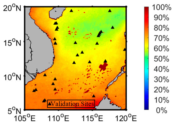
Figure 3.
The average percentage of missing data coverage. The triangles stand for the validation sites.
In situ data are obtained from the Center for Satellite Applications and Research (STAR) of the NOAA SST Quality Monitor system (iQuam) (http://www.star.nesdis.noaa.gov/sod/sst/iquam/index.html (accessed on 12 June 2023)). This study utilized data spanning from 1 January 2016 to 31 December 2019. To ensure alignment with satellite data, observations were gathered from the period of 21:00 to 24:00 each night, amounting to a total of 31,213 data points. The dataset aggregates ocean observation data obtained from seven different platforms, including ships, buoys, and others. The files retain various information, including time, longitude, latitude, measurement types, sea surface temperature, wind direction, and wind speed, among others. This system evaluates and manages the quality of the observed SST data provided by the Global Telecommunication System (GTS), classifying it into quality levels ranging from 1 to 5 [38]. This study utilizes the highest-quality observational data to calibrate the satellite data and validate the model.
3. Methods
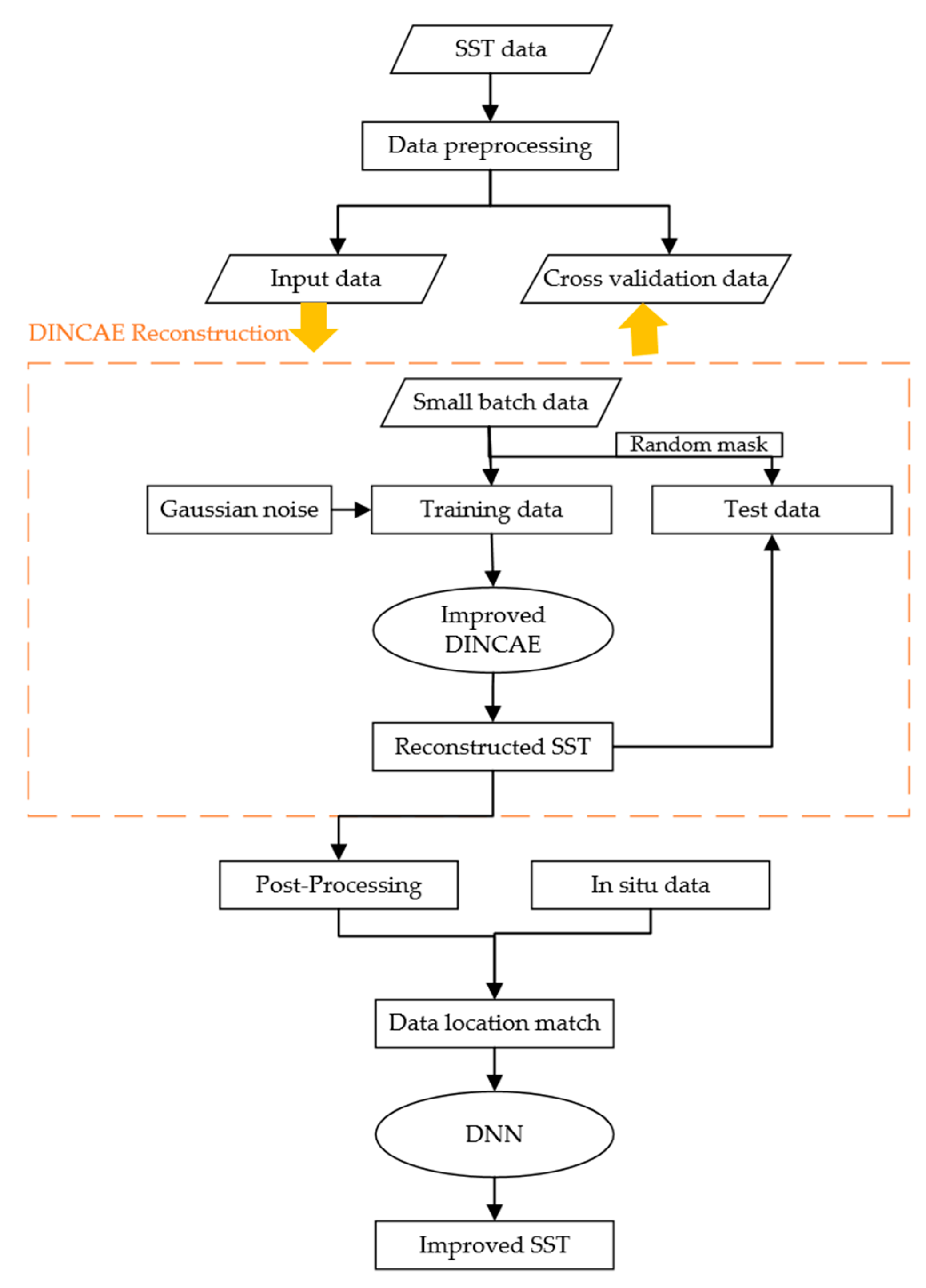
The flowchart illustrating the generation of high-precision, fully covered daily SST data from incomplete satellite data is presented in Figure 4. This approach mainly comprises two parts: (1) Reconstruction of missing data based on an I-DINCAE. Daily SST product data from FY-3C (2016–2019) were selected to construct the SST time series dataset, and an I-DINCAE algorithm was employed to build a deep-learning model for reconstructing missing data. The quality of the reconstructed data by the I-DINCAE algorithm was evaluated and compared with the results from the original DINCAE algorithm to demonstrate the reliability of the I-DINCAE algorithm in reconstructing ocean data. (2) Adjustment of the reconstructed SST through a deep neural network using in situ data. In situ data were used as reference ground truth, and the reconstructed SST data were matched spatiotemporally with in situ data. A 5-fold cross-validation method was employed to build the deep neural network model and correct the reconstructed SST data. Subsequent sections offer a comprehensive introduction to these two components.
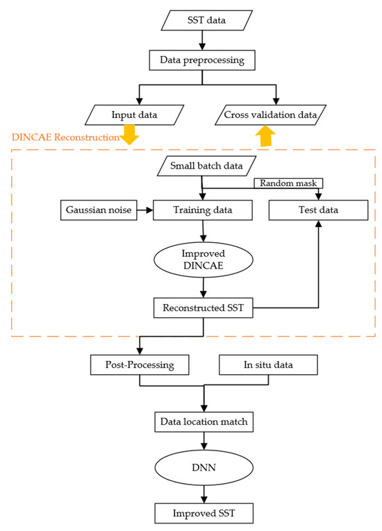
Figure 4.
The overall flowchart of the method proposed in this study.
3.1. Reconstruction of SST Based on I-DINCAE
3.1.1. Satellite Data Preprocessing
Before generating the training dataset, it is necessary to preprocess the SST data to meet the network input requirements. The size of the input dataset is 10 × 300 × 300 × 1295, representing the input dimensionality, latitude of grid points, longitude of grid points, and number of days, respectively [39]. The inputs and outputs are illustrated in Table 1.

Table 1.
List of parameters for the I-DINCAE model.
3.1.2. I-DINCAE Network Structure
The Data Interpolation Convolutional Autoencoder (DINCAE) comprises an encoder and a decoder. To extract the main features of the input data, the encoder maps the input data to the latent space through a series of convolutional and pooling layers [40]. Then, the decoder maps the representations in the latent space back to the original input space, aiming to accurately reconstruct the original input data. This process helps the network learn how to maintain key information from input data, guiding the neural network to learn mapping relationships to achieve reconstructed outputs.
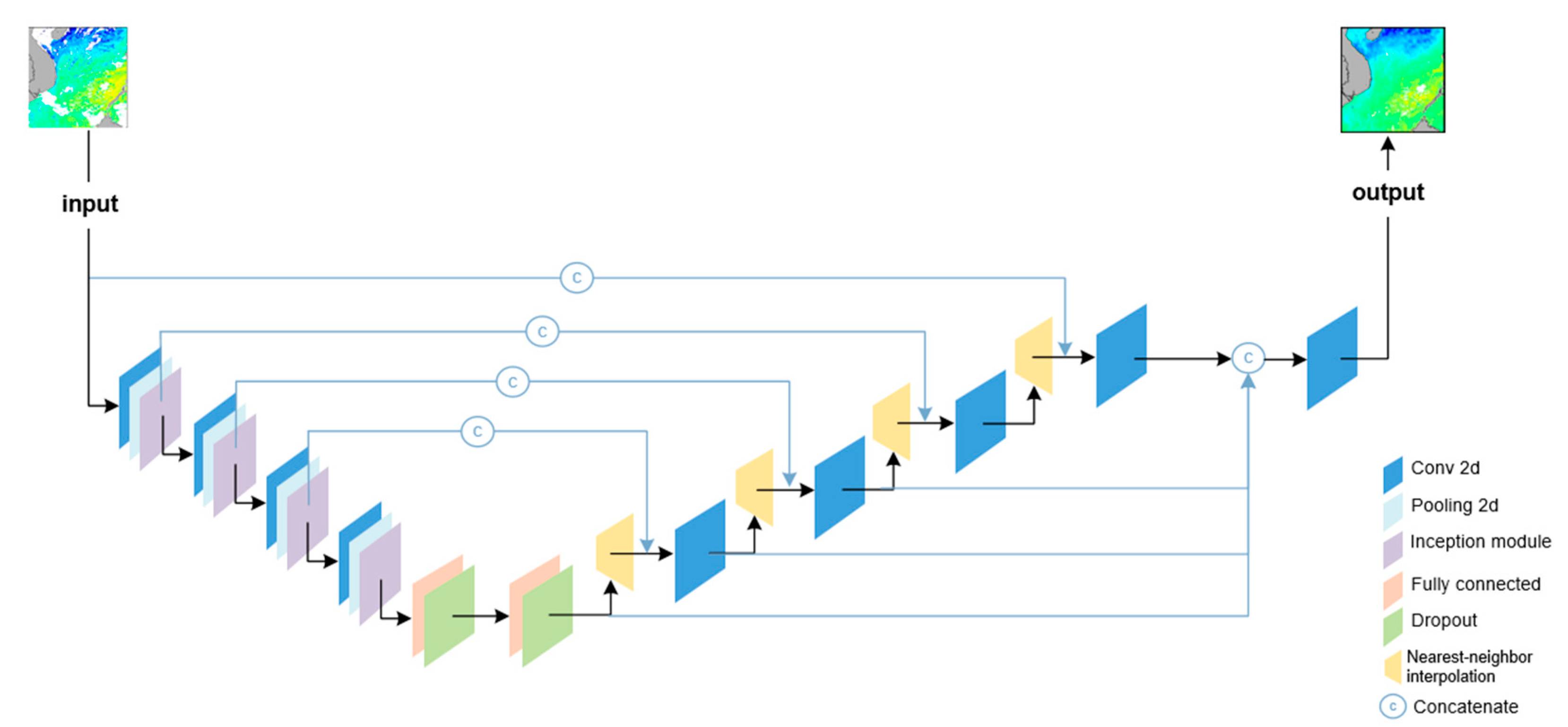
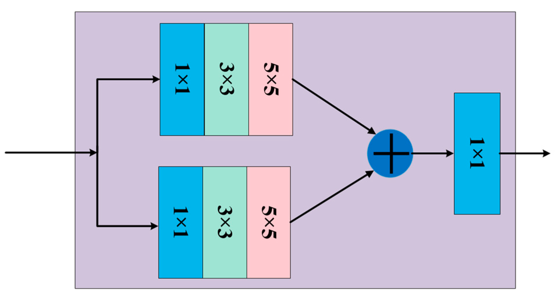
The I-DINCAE network incorporates a module for multi-scale feature extraction from the encoder outputs. By employing convolution kernels of varying sizes on the feature maps of the intermediate layer to enrich the features learned by the model, these results are concatenated and consolidated through 1 × 1 convolutional layers. Additionally, the outputs of decoders at different levels are resampled and concatenated to form a more comprehensive feature representation, enhancing the model’s accuracy in data reconstruction. The complete network structure is depicted in Figure 5, which visually illustrates the innovative design of multi-scale feature extraction in I-DINCAE. Figure 6 illustrates the inception module. This module employs two sets of 1 × 1, 3 × 3, and 5 × 5 convolution kernels, followed by fusion of the feature maps obtained from different convolution kernels, and, ultimately, inputting the fused feature maps into a 1 × 1 convolutional kernel to reduce dimensionality and enhance the network’s generalization ability.
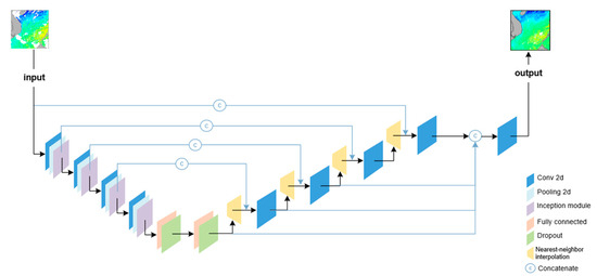
Figure 5.
Structure of the network.

Figure 6.
Inception module.
The input dataset has a size of 10 × 300 × 300 × 1295. During the training phase, due to the limitations of GPU memory, the dataset needs to be divided into multiple batches. In this study, each batch consists of 50 images, resulting in a total of 25 batches (with the last batch containing 45 images). The input data are fed into the model as an array of size 10 × 300 × 300 × 50. The network structure of DINCAE is divided into five parts (Figure 5): the input layer, encoding layer, fully connected layer, decoding layer, and output layer. The input layer is used to receive the training dataset (during the training phase) and the testing dataset (during the reconstruction phase). In the input layer, noise is randomly added to the data. In the encoding layer, the convolutional kernel size is (3 × 3); the size of the pooling layer is (2 × 2); and the stride size is (2 × 2). The encoder extracts image features through convolutional layers and max pooling layers, gradually capturing information from a larger receptive field. The filter sizes are 16, 24, 36, and 54, respectively. The fully connected layer is used to non-linearly combine the extracted features. Two fully connected layers are configured to have sizes of N/5 and N, respectively. The decoder utilizes transposed convolutional layers and interpolation layers with nearest-neighbor interpolation to perform up-sampling of feature maps. To better capture fine-scale information lost in the encoding layer and fully connected layers, the output of the pooling layer is skipped and connected directly to the interpolation layer for up-sampling. The output size is 300 × 300 × 2, which includes the reciprocal of the scaled SST expected error variance () and the logarithm of the expected error variance (). The formulae for the reconstructed SST anomalies () and their corresponding error variances () are as follows:
where = 10 and = , introducing these two constants to avoid division by zero. The subscripts i and j represent the position of each grid, and max and min denote the maximum and minimum functions.
During the process of reconstructing missing data using I-DINCAE, the model determines the usage of data based on whether the data generator is marked for training or testing mode during invocation. In training mode, the data generator introduces noise to the input data to simulate missing data, thereby increasing the randomness of the training process. In the testing mode, the data generator applies randomly selected cloud masks to mask the input data (i.e., simulating missing data by randomly selecting a cloud coverage scenario from a mini-batch), where the masked data are used for computing the loss. Throughout this process, the model continually optimizes to achieve the best reconstruction results. The loss function of the convolutional autoencoder is:
where and N are the occluded data of each grid and the number of occluded data during optimization, respectively. The first item is calculated from the standard deviation of error. The second item is to reduce the variance of the error standard deviation, which is a regularization term used to punish overestimation behavior and prevent overfitting. The third term is to normalize a constant (i.e., ignore the term).
To mitigate overfitting during neural network training, four methods proposed by the DINCAE model are utilized: (1) introducing dropout to randomly deactivate neurons; (2) adding Gaussian noise to the input data; (3) incorporating regularization terms into the Adam optimizer and adding penalty terms to the loss function to constrain model complexity; And (4) using the Leaky-RELU function instead of the traditional RELU function to alleviate the speed of gradient descent. The Gaussian noise parameter, dropout parameter, and regularization parameter are set to 0.05, 0.3, and 0, respectively.
3.2. Improvement for Reconstructed SST Data
The deviation between satellite data and in situ data, especially the difference between data with relatively low accuracy, may affect the accuracy of the final data to some extent. Deep neural networks, by learning intricate non-linear network structures, can approximate complex functions more accurately, thereby better describing the complex relationships between data. Importantly, deep neural network models can automatically extract key factors influencing data discrepancies by learning features from a large number of sample data, and establish non-linear mapping relationships between these factors and data discrepancies. The model can automatically adjust the predicted results based on input data to reduce the discrepancies and improve the accuracy of the final data. Therefore, it is adopted to establish the relationship between reconstructed SST and in situ data, while considering their time and geographic location information [29,41,42]. The main purpose of the improvement is to correct the deviation between the reconstructed SST data and the in situ data, thereby improving the data accuracy at the pixel level and ultimately producing a higher precise SST dataset.
3.2.1. Data Matching
Based on the location information of the measurement data, this study matched corresponding pixels within a set time window of 1.5 h using the iQuam SST dataset, resulting in a total of 31,213 data points being matched. Among them, 80% of the data was randomly selected as the training set, and the remaining 20% was used as the test set. Figure 7 illustrates the distribution of matched data points. The data almost cover the entire research area.
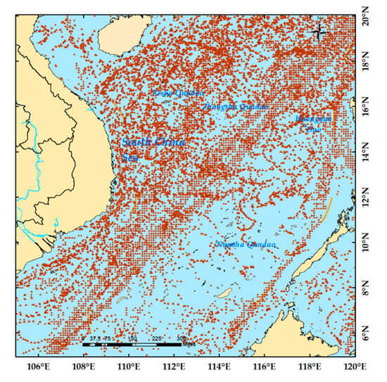
Figure 7.
Distribution map of matchup data points. Blue represents the ocean, orange represents land, red triangles indicate the locations of in-situ points.
Due to the different units of input data, it is necessary to eliminate differences between dimensions. Standardized normal distribution data were obtained by the standard normalization method. The normalization parameters are calculated as follows:
where x is the original input parameter value, µ is the mean of the parameter, and σ signifies the standard deviation.
3.2.2. Deep Neural Network
The backpropagation algorithm, serving as the central element of DNN, continually adjusts the numerical values of w and b, to minimize the error until it satisfies the accuracy requirements. Through continuous training, the loss function decreases, and the minimum parameter value is used as the model parameter. The choice of structural parameters can also influence the training outcomes under various practical scenarios. Furthermore, the selection of suitable loss functions and optimizers can enhance the accuracy of network models and expedite network training. The calculation formula for weights and biases in the backpropagation algorithm is:
where w* and w represent the updated and previous weights, respectively; b* and b are the updated and previous biases, respectively; α is the manually set learning rate; and denotes the model’s loss function. Through successive iterations of gradient descent, the optimal parameters w* and b* are attained.
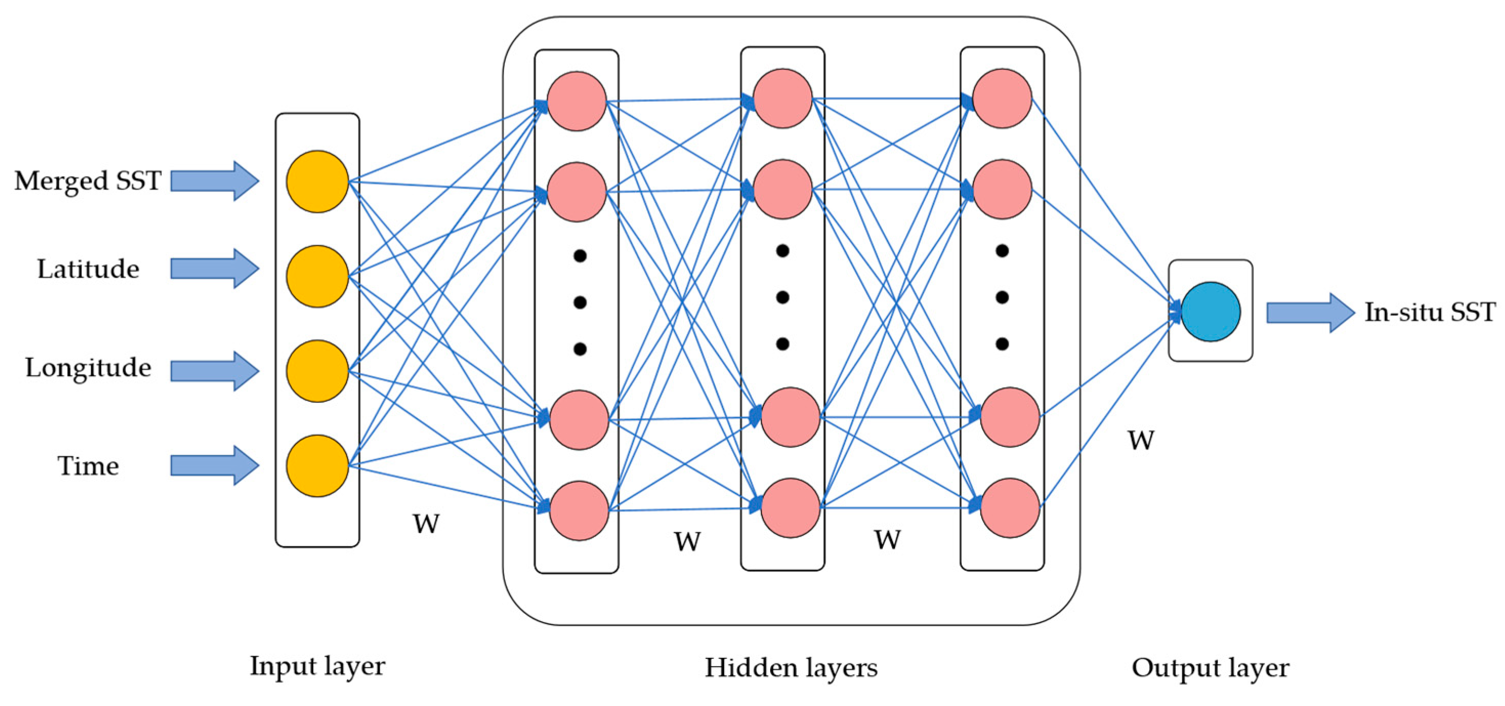
Figure 8 displays the structure of the model. This model is a 5-layer DNN model, with the first layer being the input layer, the second layer consisting of 16 hidden nodes, the third layer consisting of 32 hidden nodes, the fourth layer consisting of 64 hidden nodes, and the final output layer consisting of 1 hidden node. In this network, the inputs are latitude, longitude, time, and reconstructed SST temperature values, while the output is in situ measured data. During training, a five-fold cross-validation method is employed, dividing the training dataset into five non-overlapping subsets. Each subset alternates as the validation dataset, while the remaining four subsets are combined as the training dataset, conducting five independent experiments to assess the model’s generalization capability more robustly. Throughout the training process, the model is trained using a backpropagation algorithm, automatically adjusting parameters. Through multiple iterations of training, an optimal model is ultimately determined. Finally, the model’s performance is evaluated using an independent test dataset. The model selects the ReLU function and utilizes the Adam optimizer for optimization.
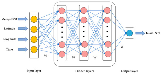
Figure 8.
Structure of a deep neural network model.
4. Results and Discussion
4.1. Validation of Reconstructed SST
To evaluate the accuracy of the reconstruction method, cross-validation was performed. In this process, cloud masks were extracted from the first 50 images of the SST data time series, and these masks were randomly applied to the last 50 images to generate the validation dataset. The validation dataset was not involved in the training and reconstruction processes. The cross-validation set comprised 1,048,575 valid overlapping pixels.
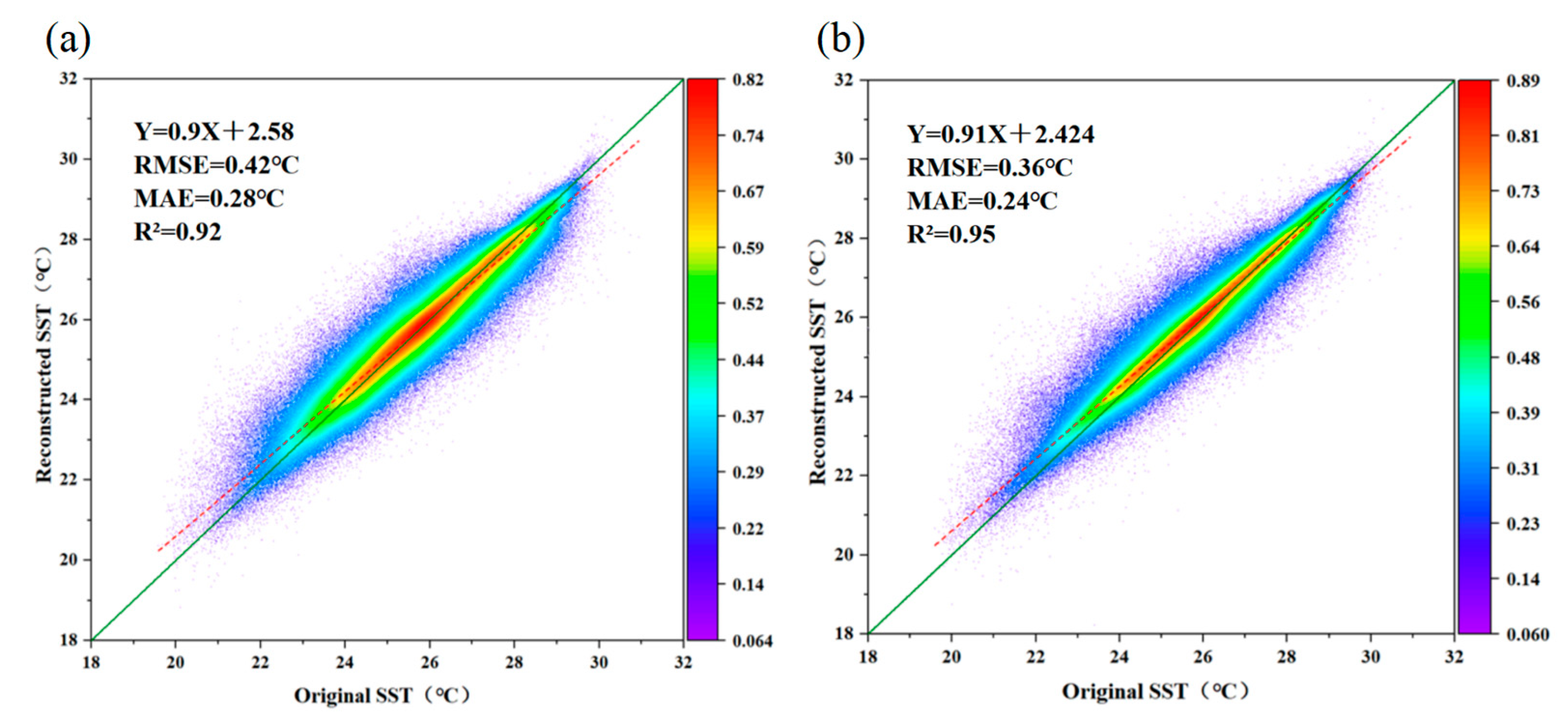
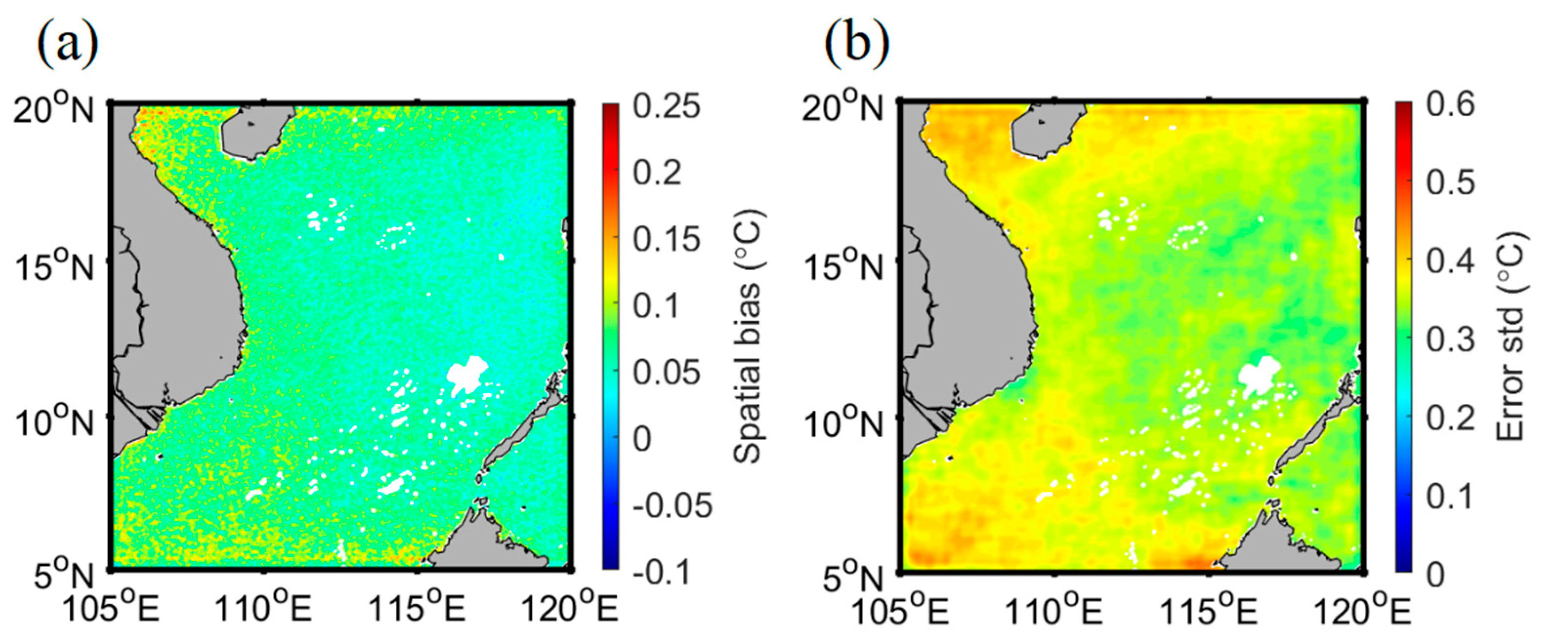
The model underwent 1000 iterations, generating a reconstruction output every 10 iterations. The reconstructed data and raw data generated by the DINCAE algorithm, as well as the I-DINCAE algorithm, were evaluated for relevant parameters, including the determination coefficient (R2), Root Mean Square Error (RMSE), and Mean Absolute Error (MAE). The correlation between the reconstructed data using the DINCAE algorithm and the original data is 0.92, with an RMSE of 0.42 °C and an MAE of 0.28 °C. The I-DINCAE algorithm exhibits a higher correlation, reaching 0.95, with an RMSE of 0.36 °C and an MAE of 0.24 °C. The scatter density plot in Figure 9 illustrates the distribution of the data, with color coding reflecting the frequency of the scatter. Each scatter represents a pair of values from the original data and the corresponding reconstructed data. The color depth indicates the frequency of the combination. By observing the distribution in the graph, one can intuitively grasp the relationship and differences between the reconstructed data and the original data. It is noteworthy that the I-DINCAE algorithm demonstrates a lower RMSE and is closer to the one-to-one fitting line. The spatial distribution of errors (mean bias and standard deviation) between the reconstructed SST and in situ data is shown in Figure 10. It can be seen that the average deviation and standard deviation of error in coastal areas are relatively high.
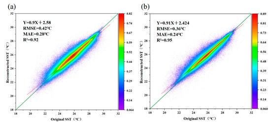
Figure 9.
Scatter density maps of reconstructed data and corresponding original data: (a) DINCAE reconstructed SST, and (b) I-DINCAE reconstructed SST. The color code represents the scatter frequency. The red dashed line represents the best-fit line, and the green solid line represents the 1:1 regression line.
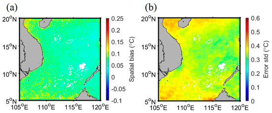
Figure 10.
The spatial distribution of (a) mean bias and (b) error standard deviation.
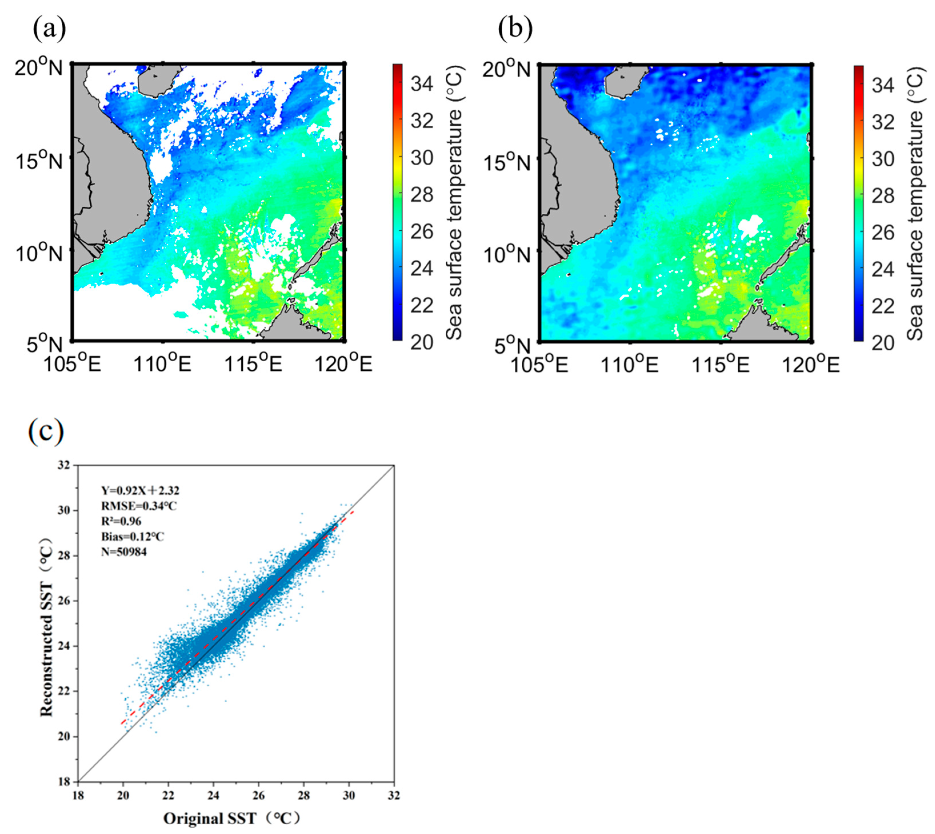
To further verify the spatial reconstruction capability, data from 20th December 2019 were selected, and the spatial distribution of the original and reconstructed data was compared. In Figure 11, (a) represents the original SST data image, (b) depicts the reconstructed image using the I-DINCAE algorithm, and (c) shows the scatter plot of the reconstructed data and corresponding original data at the location on 20th December 2019. Figure (c) demonstrates a correlation of 0.96, RMSE of 0.34 °C, and a bias of 0.12 °C between the reconstructed data and the original data, indicating a good consistency between them. From the figure, it is evident that the reconstructed results can reflect the distribution trend of the original SST image. During winter, the SST in coastal areas is lower compared to that in nearby ocean regions, which is consistent with the difference in heat capacity between seawater and land.
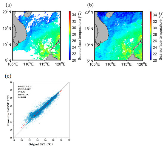
Figure 11.
Daily reconstruction on 20 December 2019: (a) the original SST, (b) the I-DINCAE reconstructed SST, and (c) the scatter plot of the original SST and reconstructed SST.
4.2. Adjustment of the Reconstructed SST
To verify the accuracy of the adjusted SST, the test dataset was fed into the trained DNN model, and the RMSE and MAE between the temperature values generated by the model and the in situ data were calculated. These error metrics provide important information for evaluating the performance of the DNN model and the accuracy of reconstructed SST. The results are detailed in Table 2. The RMSE and MAE of the reconstructed data are 1.826 °C and 1.415 °C, respectively, showing significant discrepancies with the measured data. After a calibration by the DNN model, the RMSE and MAE become 0.466 °C and 0.296 °C, respectively. From the results, it is evident that the accuracy of the adjusted SST data has improved significantly.

Table 2.
Comparison of accuracy before and after improvement.
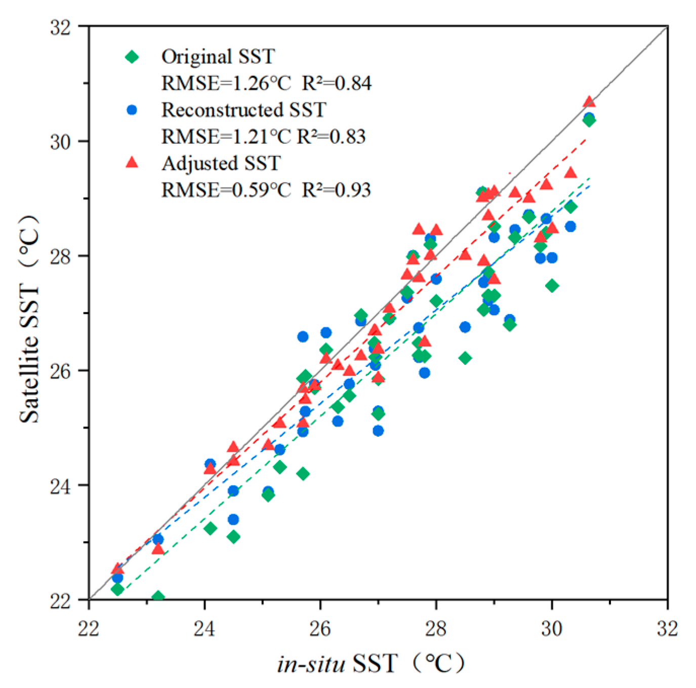
To further validate the effectiveness of the DNN model, SST data from four different dates representing different seasons (1 March 2019, 22 June 2019, 24 September 2019, and 20 December 2019) were selected to assess the correlation between the original data, reconstructed data, and adjusted data with in situ data. These four days’ data were not used for training. Among these four days, a total of 42 in situ data points spatially and temporally matched the satellite SST data. The spatial distribution of these points is shown in Figure 1. Figure 12 illustrates the correlation between the original data, reconstructed data, and adjusted data with in situ data. The R-squared value between the original data and in situ data is 0.84, with an RMSE of 1.26 °C. The R-squared value for the reconstructed data compared to in situ data is 0.83, with an RMSE of 1.21 °C. The adjusted data have an R-squared value of 0.93 and an RMSE of 0.59 °C when compared to the in situ data. The adjusted SST data (red) have the highest consistency with the in situ data.
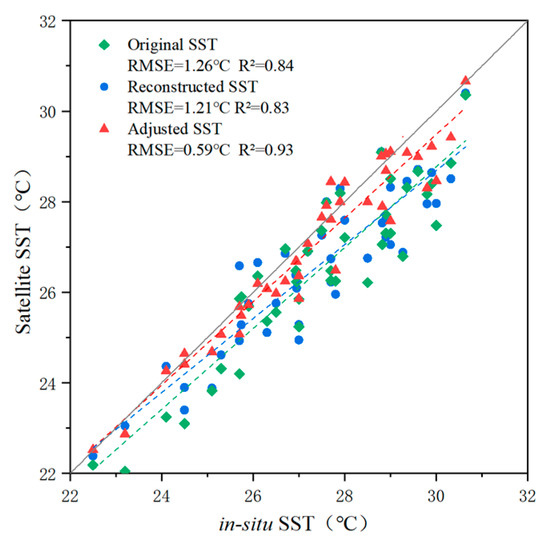
Figure 12.
Validation of satellite SST with in situ data; green, blue, and red represent the original data, reconstructed data, and adjusted data respectively. The scatter indicates the corresponding values, the dashed line represents the fitted lines, and the gray solid line represents the 1:1 line.
4.3. Seasonal Analysis on Improved Reconstructed SST
A seasonal analysis was conducted on the daily reconstructed SST data for January, April, July, and October 2019. Figure 13 illustrates the spatial distribution of SST products generated in different seasons. It can be visually observed that the SST in the South China Sea exhibits significant seasonal variations, influenced by factors such as solar radiation, air–sea heat exchange, and ocean currents, resulting in higher temperatures in summer and lower temperatures in winter. Moreover, there exists a spatial gradient in SST across the South China Sea, influenced by factors including ocean currents, coastal geography, and distance from land. Typically, temperatures are higher in the central and southern regions compared to the northern regions.
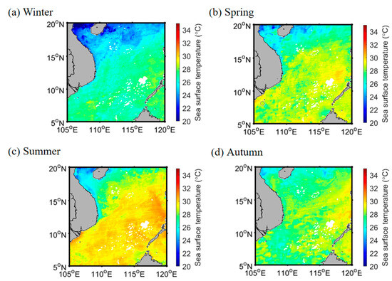
Figure 13.
Seasonal spatial distribution of sea surface temperature: (a) the reconstructed SST on 5 January 2019; (b) the reconstructed SST on 5 April 2019; (c) the reconstructed SST on 24 July 2019; and (d) the reconstructed SST on 23 October 2019.
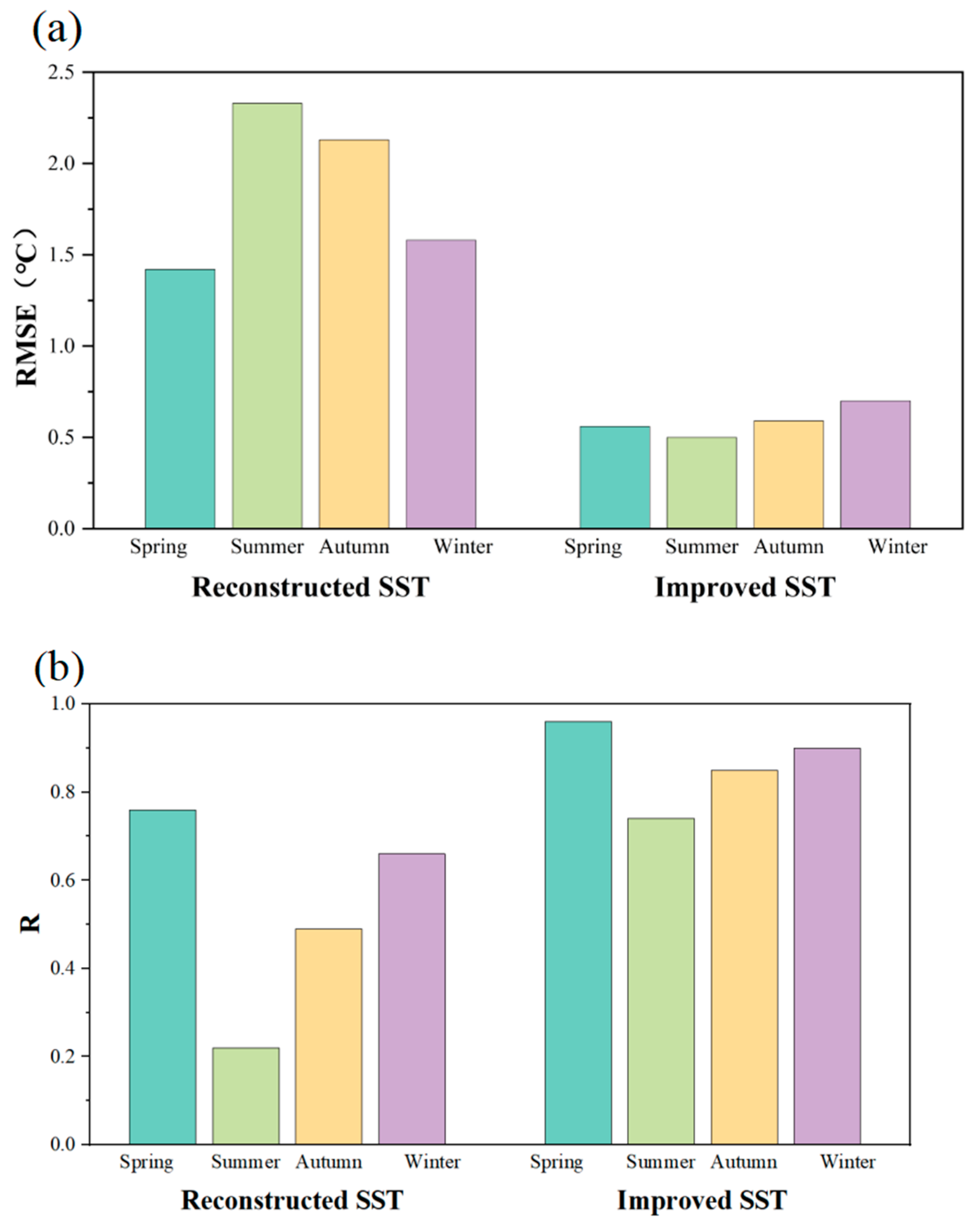
Utilizing the I-DINCAE method for reconstructing SST data and adjusting SST data through deep neural networks, the RMSE and correlation coefficient (R) of SST data generated in different seasons were compared using on-site measurement data as the real benchmark (Figure 14). In spring, the RMSE decreased from 1.42 °C to 0.56 °C, while the R increased from 0.76 to 0.96. In summer, the RMSE decreased from 2.33 °C to 0.50 °C, with the R increasing from 0.22 to 0.74. For autumn, the RMSE decreased from 2.13 °C to 0.59 °C, while the R increased from 0.49 to 0.85. In winter, the RMSE decreased from 1.58 °C to 0.70 °C, with the R increasing from 0.66 to 0.90. These results indicate that the data generated by the I-DINCAE method and deep neural network method exhibit a good correlation with the measured data, with a correlation coefficient ranging from 0.72 to 0.95. The RMSE of the generated SST data has also significantly decreased. This suggests that the adjusted SST data have a good consistency and accuracy with the measurement data. However, the performance of summer data in this evaluation was subpar, which may be primarily attributed to weather conditions. Due to the instability of summer weather conditions, the high masking rate during data collection affects the training and performance of the model. Additionally, the relatively low coverage during summer may pose challenges with data loss and noise, thereby impacting the accurate reconstruction of the data. Hence, under such weather conditions, the decrease in data quality may affect the accuracy of predictions in summer.
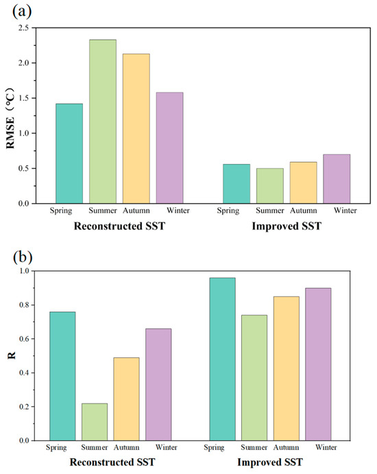
Figure 14.
Comparison of (a) RMSE and (b) R between in situ data and improved data from different seasons.
5. Discussion
This study employed the I-DINCAE algorithm to reconstruct the SST data, effectively filling in the data gaps and increasing the coverage of the SST data to nearly 100%. Subsequently, further enhancements were made to the reconstructed SST through a deep neural network (DNN). By correcting significant discrepancies between SST in satellite data and measured data, the accuracy of the SST data was enhanced, resulting in more precise SST data. Although a certain level of accuracy was achieved, there are still areas for research and improvement:
(1) The autoencoder in I-DINCAE smooths the data, inevitably leading to the loss of some small-scale information. Although I-DINCAE can capture non-linear and abrupt relationships, thereby addressing some issues, future research could involve inputting multiple variables (such as temperature, salinity, wind field, etc.) into I-DINCAE to explore deeper relationships and establish a more comprehensive deep-learning model.
(2) The input matrix shape of the I-DINCAE model, determined by the fully connected layers, restricts the model from training and predicting in a single region, thus reducing its versatility. To predict in different regions, a new model needs to be trained for each region of interest. However, the applicability of this model is limited due to the lengthy training process, requiring long data sequences and iterations, as well as complex data and operational requirements. Future improvements could involve enhancing the model’s generalization capability and versatility by simultaneously extracting features from multiple geographical regions.
(3) Due to the limited availability of data sources used in the experiment, there was a shortage of effective data during the summer, resulting in a lower reconstruction accuracy during that season, which imposed certain limitations on the accuracy of the reconstruction results. Therefore, considering other sources of SST products and integrating them with existing data could improve the coverage of effective data and achieve better reconstruction results.
(4) Moreover, this study only utilized four years of SST data due to data constraints. To gain a more comprehensive understanding of SST trends and patterns, future research could extend to longer time series data.
6. Conclusions
This study proposes a deep-learning-based data reconstruction method that is aimed at generating high-resolution seamless daily SST data for the South China Sea from 2016 to 2019. Initially, the I-DINCAE algorithm is employed to reconstruct missing FY-3C SST data, effectively enhancing the coverage of SST products. A quantitative analysis demonstrates the effectiveness of the I-DINCAE algorithm in reconstructing SST data, with the R2 of 0.95, the RMSE of 0.36 °C, and the MAE of 0.24 °C, outperforming the DINCAE algorithm. Subsequently, by introducing a DNN model and in situ measurements, the reconstructed SST data are further refined to improve the accuracy of the SST products. Compared to the in situ measurements, the results after calibration show the RMSE of 0.466 °C and MAE of 0.296 °C. Lastly, at the seasonal scale, SST variations exhibit pronounced seasonal characteristics, with higher sea surface temperatures influenced by warm currents and tropical monsoons in summer, and relatively lower temperatures in the northern South China Sea due to monsoons and the upwelling of cold water in winter. This study not only advances the application of the DINCAE algorithm but also refines SST data through the introduction of a DNN, providing comprehensive and accurate SST information for the South China Sea. The method can be used for global-scale sea surface temperature reconstruction and further contributes to research and applications in global and regional climate studies.
Author Contributions
Conceptualization, Z.L. and D.Z.; methodology, Z.L. and X.Z.; validation, Z.L., Y.G. and D.Z.; writing—original draft preparation, Z.L., D.Z. and X.Z.; writing—review and editing, D.W., D.Z. and X.Z. All authors have read and agreed to the published version of the manuscript.
Funding
This research was funded by the Key Research and Development Program sponsored by the Ministry of Science and Technology (MOST) 2023YFC3107701 and 2023YFC3107901, and the National Natural Science Foundation of China (No. 42375143), and was also funded by the Key Laboratory of Smart Earth, NO. KF2023YB03-03.
Data Availability Statement
The data underlying the results presented in this paper can be obtained from the authors upon reasonable request. The data are not publicly available due to privacy restrictions.
Acknowledgments
The authors would like to acknowledge the anonymous reviewers for their valuable comments.
Conflicts of Interest
The authors declare no conflicts of interest.
References
- Xu, B.; Yu, J.; Zhang, L.; Shi, C.; Zhou, Z. Research progress on global sea surface temperature fusion. Prog. Meteorol. Technol. 2018, 8, 164–170. [Google Scholar]
- Park, S.; Deser, C.; Alexander, M.A. Estimation of the Surface Heat Flux Response to Sea Surface Temperature Anomalies over the Global Oceans. J. Clim. 2005, 18, 4582–4599. [Google Scholar] [CrossRef]
- Dunstan, P.K.; Foster, S.D.; King, E.; Risbey, J.; O’Kane, T.J.; Monselesan, D.; Hobday, A.J.; Hartog, J.R.; Thompson, P.A. Global Patterns of Change and Variation in Sea Surface Temperature and Chlorophyll a. Sci. Rep. 2018, 8, 14624. [Google Scholar] [CrossRef] [PubMed]
- Song, W.; Zhang, P.; Sun, L. Research on the Sea Surface Temperature Reconstruction Method of Fengyun Polar Orbit Meteorological Satellite Based on DINEOF. J. Oceanogr. Res. 2022, 40, 10. [Google Scholar]
- Shesu, R.V.; Bhaskar, T.V.S.U.; Rao, E.P.R.; Ravichandran, M.; Rao, B.V. An Improved Method for Quality Control of in Situ Data from Argo Floats Using α Convex Hulls. MethodsX 2021, 8, 101337. [Google Scholar] [CrossRef] [PubMed]
- Hu, Z. Research on Sea Surface Temperature Prediction Based on Non-stationary Time Series; Shanghai Ocean University: Shanghai, China, 2021. [Google Scholar]
- Cao, M.; Mao, K.; Yan, Y.; Shi, J.; Wang, H.; Xu, T.; Fang, S.; Yuan, Z. A New Global Gridded Sea Surface Temperature Data Product Based on Multisource Data. Earth Syst. Sci. Data 2021, 13, 2111–2134. [Google Scholar] [CrossRef]
- Everson, R.; Cornillon, P.; Sirovich, L.; Webber, A. An Empirical Eigenfunction Analysis of Sea Surface Temperatures in the Western North Atlantic. J. Phys. Oceanogr. 1997, 27, 468–479. [Google Scholar] [CrossRef]
- Huang, X.-Y. Variational Analysis Using Spatial Filters. Mon. Weather. Rev. 2000, 128, 2588–2600. [Google Scholar] [CrossRef]
- Reynolds, R.W.; Smith, T.M. Improved Global Sea Surface Temperature Analyses Using Optimum Interpolation. J. Clim. 1994, 7, 929–948. [Google Scholar] [CrossRef]
- Müller, D. Estimation of Algae Concentration in Cloud Covered Scenes Using Geostatistical Methods. In Proceedings of the ENVISAT Symposium, Montreux, Switzerland, 23–27 April 2007. [Google Scholar]
- Feng, Y.; Lei, X.; Lu, Y. Applying spatial statistics theory to interpret the missing areas of remote sensing image information. J. Remote Sens. 2004, 8, 317–322. [Google Scholar]
- Yu, X.; Ma, A. A study on remote sensing missing data of sea surface chlorophyll based on Kriging spatial interpolation. Surv. Mapp. Bull. 2013, 12, 47–50. [Google Scholar]
- Beckers, J.M.; Rixen, M. EOF Calculations and Data Filling from Incomplete Oceanographic Datasets. J. Atmos. Ocean. Technol. 2003, 20, 1839–1856. [Google Scholar] [CrossRef]
- Zhou, F.; Tang, S.; Han, X.; Song, X.; Cao, G. Research on the reconstruction method of surface temperature using cloud based remote sensing. Remote Sens. Land Resour. 2021, 33, 78–85. [Google Scholar]
- Li, Y.; Sun, W.; Zhang, J.; Meng, J.; Zhao, Y. Reconstruction of Arctic SST Data and Generation of Multi-Source Satellite Fusion Products with High Temporal and Spatial Resolutions. Remote Sens. Lett. 2021, 12, 695–703. [Google Scholar] [CrossRef]
- Ćatipović, L.; Matić, F.; Kalinić, H. Reconstruction Methods in Oceanographic Satellite Data Observation—A Survey. J. Mar. Sci. Eng. 2023, 11, 340. [Google Scholar] [CrossRef]
- He, H.; Li, Y.; Wang, Y.; Song, X.; Liu, X. Reconstruction of chlorophyll-a concentration field in the East China Sea using empirical orthogonal function data interpolation method. Oceanogr. Res. 2013, 31, 10–15. [Google Scholar]
- Guo, J.; Song, J. Research on the Reconstruction Method of Remote Sensing Chlorophyll Data in the East China Sea. Remote Sens. Technol. Appl. 2016, 31, 939–949. [Google Scholar]
- Alvera-Azcárate, A.; Barth, A.; Parard, G.; Beckers, J.-M. Analysis of SMOS Sea Surface Salinity Data Using DINEOF. Remote Sens. Environ. 2016, 180, 137–145. [Google Scholar] [CrossRef]
- Sheng, Z.; Shi, H.; Ding, Y. Reconstruct missing satellite remote sensing sea surface temperature data using the DINEOF method. Prog. Mar. Sci. 2009, 27, 243–249. [Google Scholar]
- Jouini, M.; Lévy, M.; Crépon, M.; Thiria, S. Reconstruction of Satellite Chlorophyll Images under Heavy Cloud Coverage Using a Neural Classification Method. Remote Sens. Environ. 2013, 131, 232–246. [Google Scholar] [CrossRef]
- Park, J.; Kim, H.-C.; Bae, D.; Jo, Y.-H. Data Reconstruction for Remotely Sensed Chlorophyll-a Concentration in the Ross Sea Using Ensemble-Based Machine Learning. Remote Sens. 2020, 12, 1898. [Google Scholar] [CrossRef]
- Barth, A.; Alvera-Azcárate, A.; Licer, M.; Beckers, J.-M. DINCAE 1.0: A Convolutional Neural Network with Error Estimates to Reconstruct Sea Surface Temperature Satellite Observations. Geosci. Model Dev. 2020, 13, 1609–1622. [Google Scholar] [CrossRef]
- Krasnopolsky, V.; Nadiga, S.; Mehra, A.; Bayler, E.; Behringer, D. Neural Networks Technique for Filling Gaps in Satellite Measurements: Application to Ocean Color Observations. Comput. Intell. Neurosci. 2015, 2016, e6156513. [Google Scholar] [CrossRef]
- Li, J.; Sun, W.; Zhang, J. Reconstruct Infrared Sea Surface Temperature Data Based on an Improved DINCAE Method. In Proceedings of the IGARSS 2023—2023 IEEE International Geoscience and Remote Sensing Symposium, Pasadena, CA, USA, 16–21 July 2023; pp. 4120–4123. [Google Scholar]
- Xiong, Y. Deep Learning Based Data Reconstruction of Chlorophyll a and Its Spatiotemporal Variation Characteristics. Master’s Thesis, Guilin University of Technology, Guilin, China, 2023. [Google Scholar]
- Ye, H.; Tang, S.; Yang, C.; Chen, C. Reconstruction of Daily MODIS/Aqua Chlorophyll-a Concentration in Turbid Estuarine Waters Based on Attention U-NET. Remote Sens. 2023, 15, 546. [Google Scholar] [CrossRef]
- Jung, S.; Yoo, C.; Im, J. High-Resolution Seamless Daily Sea Surface Temperature Based on Satellite Data Fusion and Machine Learning over Kuroshio Extension. Remote Sens. 2022, 14, 575. [Google Scholar] [CrossRef]
- Ai, B.; Wen, Z.; Jiang, Y.; Gao, S.; Lv, G. Sea Surface Temperature Inversion Model for Infrared Remote Sensing Images Based on Deep Neural Network. Infrared Phys. Technol. 2019, 99, 231–239. [Google Scholar] [CrossRef]
- Sun, G.; Guan, D.; Zhao, D.; Wang, X.; Wang, X. Evaluation of the Applicability of TMI Sea Surface Temperature Data in the South China Sea. J. Mar. Environ. Sci. 2014, 33, 311–317. [Google Scholar]
- Ni, J. Information Extraction and Change Driving Force Analysis of Jiangsu Coastal mudflat Based on Satellite Images; Nan-jing University of Information Engineering: Nanjing, China, 2023. [Google Scholar]
- Morak-Bozzo, S.; Merchant, C.J.; Kent, E.C.; Berry, D.I.; Carella, G. Climatological Diurnal Variability in Sea Surface Temperature Characterized from Drifting Buoy Data. Geosci. Data J. 2016, 3, 20–28. [Google Scholar] [CrossRef]
- Zhang, C.; Li, S.; Liu, H.; Li, B.; Song, J. Inspection of Sea Surface Temperature Products for the Fengyun 3 Satellite Microwave Imager. J. Equip. Environ. Eng. 2021, 18, 115–123. [Google Scholar]
- Zhang, M.; Wang, S.; Qin, D.; Qiu, H.; Tang, S. Algorithm and accuracy testing of the FY-3C microwave imager sea surface temperature product. J. Remote Sens. 2018, 22, 713–722. [Google Scholar]
- Wang, S.; Cui, P.; Zhang, P.; Yang, Z.; Rao, M.; Hu, X.; Lu, F.; Liu, J. Development of FY-3 satellite VIRR sea surface temperature products. J. Shanghai Aero-Space 2017, 34, 79–84. [Google Scholar]
- Han, Z.; He, Y.; Liu, G.; Perrie, W. Application of DINCAE to Reconstruct the Gaps in Chlorophyll-a Satellite Observations in the South China Sea and West Philippine Sea. Remote Sens. 2020, 12, 480. [Google Scholar] [CrossRef]
- Xu, F.; Ignatov, A. In Situ SST Quality Monitor (iQuam). J. Atmos. Ocean. Technol. 2014, 31, 164–180. [Google Scholar] [CrossRef]
- Luo, X. Research on the Algorithm for Reconstructing Chlorophyll a Data from Yellow Sea and Bohai Sea Satellite Remote Sensing; Dalian Ocean University: Dalian, China, 2022. [Google Scholar]
- Yan, X.; Gao, Z.; Jiang, Y.; He, J.; Yin, J.; Wu, J. Application of Synthetic DINCAE–BME Spatiotemporal Interpolation Framework to Reconstruct Chlorophyll–a from Satellite Observations in the Arabian Sea. J. Mar. Sci. Eng. 2023, 11, 743. [Google Scholar] [CrossRef]
- Gao, M.; Huang, X.; Wang, F.; Zhang, H.; Zhao, H.; Gao, X. Inversion of sea surface salinity based on deep neural networks. J. Prog. Mar. Sci. 2022, 40, 496–504. [Google Scholar]
- Zhang, D. Research on the Reconstruction of Marine Chlorophyll a Concentration Data Based on Deep Learning; China University of Petroleum (East China): Shandong, China, 2020. [Google Scholar]
Disclaimer/Publisher’s Note: The statements, opinions and data contained in all publications are solely those of the individual author(s) and contributor(s) and not of MDPI and/or the editor(s). MDPI and/or the editor(s) disclaim responsibility for any injury to people or property resulting from any ideas, methods, instructions or products referred to in the content. |
© 2024 by the authors. Licensee MDPI, Basel, Switzerland. This article is an open access article distributed under the terms and conditions of the Creative Commons Attribution (CC BY) license (https://creativecommons.org/licenses/by/4.0/).

