Article

Range-Spread Target Detection Networks Using HRRPs

1
School of Electronics and Communication Engineering, Shenzhen Campus of Sun Yat-sen University, Shenzhen 518107, China
2
School of Electronics and Communication Engineering, Sun Yat-sen University, Guangzhou 510275, China
3
Guangdong Laboratory of Artificial Intelligence and Digital Economy (SZ), Shenzhen 518107, China
*
Author to whom correspondence should be addressed.
Remote Sens. 2024, 16(10), 1667; https://doi.org/10.3390/rs16101667
Submission received: 14 March 2024 / Revised: 2 May 2024 / Accepted: 7 May 2024 / Published: 8 May 2024
(This article belongs to the Topic Radar Signal and Data Processing with Applications)

Abstract

:
Range-spread target (RST) detection is an important issue for high-resolution radar (HRR). Traditional detectors relying on manually designed detection statistics have their performance limitations. Therefore, in this work, two deep learning-based detectors are proposed for RST detection using HRRPs, i.e., an NLS detector and DFCW detector. The NLS detector leverages domain knowledge from the traditional detector, treating the input HRRP as a low-level feature vector for target detection. An interpretable NLS module is designed to perform noise reduction for the input HRRP. The DFCW detector takes advantage of the extracted high-level feature map of the input HRRP to improve detection performance. It incorporates a feature cross-weighting module for element-wise feature weighting within the feature map, considering the channel and spatial information jointly. Additionally, a nonlinear accumulation module is proposed to replace the conventional noncoherent accumulation operation in the double-HRRP detection scenario. Considering the influence of the target spread characteristic on detector performance, signal sparseness is introduced as a measure and used to assist in generating two datasets, i.e., a simulated dataset and measured dataset incorporating real target echoes. Experiments based on the two datasets are conducted to confirm the contribution of the designed modules to detector performance. The effectiveness of the two proposed detectors is verified through performance comparison with traditional and deep learning-based detectors.

Graphical Abstract

1. Introduction

In modern technology, radar plays an important role in environment interpretation. The increased demands of industries on sensors’ abilities promote the development of the radar system. Modern radar has evolved toward high resolution, namely high-resolution radar (HRR) [1]. Abundant information about target details is available in HRR, which enables target imaging and recognition based on the radar system. However, the high resolution of radar brings not only benefits but also challenges for traditional radar task, such as target detection [2].
In HRR, a single target does not appear as a point target in traditional low-resolution radar (LRR) but rather as a spread target consisting of multiple scattering centers. A radar with high resolution on the range dimension results in a one-dimension high-resolution range profile (HRRP) in the receiving window. The target in there is represented by several scatterers within a range window, i.e., the range-spread target (RST). The HRRP enables the observation of structural characteristics of an RST. However, the energy of an RST is spread into scatterers in different range bins, and the signal-to-noise ratio (SNR) of a single scatterer is lower than that of the whole target. Therefore, the target detection in HRR is much more difficult than in LRR.
Over the past few decades, the detection of an RST in HRR is a major concern of researchers, and significant progress has been made. To mitigate the performance degradation caused by target energy dispersion, a reasonable way is to improve the integration efficiency, namely improving the output SNR by integrating target dispersed energy as well as suppressing noise.
In [3], two types of detectors are considered for RST detection, i.e., an energy integration (EI) detector and M out of N (M/N) detector. The EI detector integrates the energy of all range bins in an HRRP indiscriminately. Therefore, not only the dispersed target energy is integrated but also the energy of noise. This could lead to performance degradation when most of the integrated range bins are noise-occupied: namely, the target scatterers are sparsely distributed in the HRRP. For the M/N detector, it is implemented in a way of double-threshold detection. The first threshold figures out range bins, which are target-occupied and the binary integrated result is compared with the second threshold to determine whether a target is present. The M/N detector is designed for sparse target, but the performance lacks robustness. The two detectors are basics of adaptive RST detection exploiting target scattering characteristic.
An enhanced EI detector is proposed in [4], which uses an optimized window to lessen the collapsing loss but requires an additional search process. Several double-threshold detectors are proposed for improvement of the M/N detector [5,6,7]. The GLRT-DT in [5] optimizes the selection of the first threshold by information criterion and energy integration is used to replace the binary integration to avoid the performance loss. However, there could be a misjudgement between range bins of target and noise, resulting in performance degradation.
In [8], the designed SDD-GLRT detector exploits an a priori assumption of the target scattering characteristic to achieve better detection performance. However, the detection performance will be degraded using mismatched priori knowledge. The ASCE-GLRT detector in [9] treats the estimation of the target scattering characteristic as a problem of sparse optimization to avoid the priori requirement, but the calculated dynamic regularization parameter is influenced by noise and will affect the performance.
The detectors in [10,11,12] perform cross-correlation between consecutive HRRPs to exploit the similarity in HRRPs. The MCOM detector in [10] proposes a nonlinear shrinkage (NLS) function for the noise reduction of HRRP to mitigate the impact of noise on cross-correlation. But the effect of NLS function for noise reduction can result in a loss of target energy and lead to performance degradation, especially for dense targets. The detector in [13] combines a time-frequency feature with sparse representation to realize target detection, which involves complicated computation. An order statistics-based detector is proposed in [14]. The range bins are sorted by energy and integrated to perform target detection. However, the calculation of the detection threshold requires iterative computation.
The above-mentioned detectors make every effort to improve the detection performance. The key idea is to distinguish the noise and target scatterers. However, in the case of a low SNR, it could be challenging, and the detection performance is usually limited.
In recent years, deep learning with its superiority is explored by researchers and applied to various radar tasks [15,16,17], including radar target detection [18].
Deep learning-based background data processing is studied to benefit radar target detection [19,20,21,22]. The proposed network in [19] is based on the convolutional neural network (CNN) and realizes a classification of background noise and clutter. However, it can only be used to serve the selection of detection methods, and further work is required. Traditional constant false alarm rate (CFAR) algorithms are improved based on deep learning [20,21,22]. In [21], the noise estimation process is optimized in the presence of masking effects. The proposed model in [22] enhances the background estimation in the presence of interfering targets using a peak sequence classification network, and targets are detected based on a CFAR regulation processor. These methods focus on the optimization of background noise processing which is beneficial to the target detection, but the detection performance is still limited by the used CFAR methods.
Two detection networks are proposed in [23,24]. They are based on the raw radar data and eliminate the need for the preprocessing of a radar signal. In [23], a model for the multitask target detection network is proposed. The input is across three dimensions, corresponding to sampling in the range, pulse and channel. Target detection and motion parameters estimation such as range, velocity, and angle are realized based on the designed network. However, the extra estimation tasks will affect the detection performance, and the false alarm rate of the designed network is not considered. The proposed network in [24] is based on an artificial neural network (ANN) and takes the time-domain frequency modulated continuous wave (FMCW) signal as input. Traditional fast Fourier transform and CFAR procedures are replaced by the network, but the performance of the network requires a high SNR level to outperform a traditional CFAR detector.
The two-dimensional (2D) spectrum of radar data is commonly used for deep learning-based detectors. In [25], a deep learning-based detector is proposed to help object detection in traffic scenes. The proposed detector combines the YOLOv8 (You Only Look Once) [26] architecture with the ConvLSTM (Convolution and Long Short-Term Memory) structure and attention module to treat the time series of a range-Doppler spectrum. The additional information from the time series improves the performance of the proposed detector but also leads to the increase in computation complexity. In [27], a CNN detector is proposed based on the LENET [28], which performs target detection based on the range-Doppler spectrum. Binary labels are used to represent the hypotheses, and target detection is treated as a classification problem. However, the false alarm rate of the proposed detector is changed with SNR, which is undesirable for radar detection.
An HRRP recognition network is proposed in [29]. The time-related feature is extracted based on the combination of the CNN-based autoencoder and the LSTM structure. The classification of target HRRP and noise is based on the support vector data description (SVDD) [30] in which a hyper-sphere is established as the classification judgement condition. However, the LSTM structure is with limited performance gain. In [31], marine target detection is considered via CNN. The proposed detector takes the processed time-Doppler spectrum and amplitude information as dual-channel input. Features of input are extracted and fused for further classification. The control of the false alarm rate is discussed and realized using a variable threshold softmax classifier and false alarm controllable support vector machines (SVMs). However, the detection performance is affected by the control of the false alarm rate.
Overall, radar target detection based on deep learning is promising. Therefore, in this work, the detection of an RST is considered in the scenarios of a single HRRP and double HRRPs, and deep learning-based detectors are designed to improve the detection performance.
Two network detectors for RST detection are proposed in this paper based on different design philosophies. The first detector is a nonlinear shrinkage based detector (NLS detector). Denoising is a common method used to improve the performance of radar [32] and sonar systems [33,34,35]. Therefore, the proposed NLS detector takes the HRRP as a low-level feature vector, and an NLS module is designed for noise reduction, referring to the traditional mapping function in the MCOM detector [10]. The RST detection is regarded as a binary classification problem, and a classifier with two output neurons is introduced to obtain the classification result. Finally, the classification output is combined with a difference module to realize the control of the false alarm rate. The second detector is a deep feature cross-weighting based detector (DFCW detector). The DFCW detector, referring to the CNN-LSTM detector [29], introduces the CNN-based feature extraction module to obtain the high-level feature map of the HRRP, and target detection is treated as anomaly detection based on the SVDD. A feature cross-weighting module, considering channel and spatial information jointly, performs element-wise feature weighting in the feature map to select important features. The weighted feature map is then integrated into a statistical feature and used in SVDD to perform anomaly detection. For a double-HRRP detection scenario, a nonlinear accumulation module is designed to replace the traditional noncoherent accumulation operation and to improve the detection performance. For performance evaluation, the simulated dataset and measured dataset based on real target echoes are generated. The two datasets take into account the range-spread characteristic of the target to analyze its influence on detection performance. Finally, the effectiveness of the proposed network detectors is verified and compared with traditional and deep learning-based detectors. The contributions of this work are summarized as follows:
  • An NLS module is designed assisted by the domain knowledge of a traditional detector. The NLS module learns a data adaptive mapping function to perform noise suppression for the input HRRP. Based on the NLS module, a network detector for RST detection is proposed, which takes the denoised HRRP as a low-level feature vector and realizes target detection via binary classification.
  • A network detector for RST detection based on high-level feature extraction of HRRP is proposed. In the proposed detector, a feature cross-weighting module based on joint channel-spatial information is designed for element-wise feature weighting. A nonlinear accumulation module for the preprocessing of double-HRRP input is developed, which replaces the traditional noncoherent accumulation in a double-HRRP detection scenario and enhances the detection performance.
  • The range-spread characteristic of an RST is considered for performance evaluation. Signal sparseness in [36] is introduced for quantification, and simulated and measured datasets with different sparseness are generated. The effectiveness of the proposed detectors is verified and compared to traditional and deep learning-based detectors.

2. Methods

2.1. Detection Model

The linear frequency modulation (LFM) signal is a common waveform for radar target detection. In HRR, the transmitted LFM signal has a large bandwidth and results in a high resolution in range. For an RST, as a combination of multiple scatterers, the returned signal of the target after mixing is expressed as
s mix ( t ) = p = 1 P a p rect t τ p T exp ( j 2 π γ τ p t ) ϕ ( τ p )
where t represents the fast time within the chirp, P is the number of scatterers of the target and p indicates the index of the scatterer. The a p is the amplitude of the p-th scatterer. The rect ( t ) represents the rectangle function, and T is the duration of the chirp. The τ p is the round-trip time delay of the p-th scatterer. γ = B / T is the chirp rate and B is the bandwidth of the LFM signal. The ϕ ( τ p ) = exp ( j 2 π f c τ p j π γ τ p 2 ) is the phase term independent of t, and f c is the carrier frequency.
The HRRP in the received window of the HRR shows the one-dimensional structural information of the RST and is obtained based on the Fourier transform of the mixer output, which is expressed as
s ( f ) = p = 1 P a p sinc ( T ( f γ τ p ) ) exp ( j 2 π f c τ p )
where sinc ( x ) = sin ( π x ) / π x represents the normalized sinc function. f p R = γ τ p indicates the frequency corresponding to the range of the p-th scatterer in the HRRP. In the HRRP, each scatterer corresponds to a peak of the sinc function.
For the radar system, the received signal consists of target echo and noise from the environment and built-in system. The detection procedure determines whether a target is present in the received signal. In this work, target detection is considered using different numbers of received HRRPs and is formulated as a binary hypothesis testing:
H 0 : y q = n q H 1 : y q = s q + n q
where H 0 is the null hypothesis and H 1 is the alternative hypothesis. The q = 1 , , Q is the index of the sequence and Q = { 1 , 2 } corresponds to the detection scenarios using a single HRRP and double HRRPs. The y is the received HRRP, s is the target HRRP and n is the complex Gaussian noise. For the same target, the HRRP is determined but unknown, i.e., s 1 = s 2 = s . The two noise sequences are independent from each other.
Different scatterers of an RST are within a range window around the target center. An example of the HRRP of an RST is shown in Figure 1.
As shown in Figure 1a, the target is located in a range bin window of length L = 32 . Figure 1b shows the sampled noise in the window. The received noisy HRRP of the radar is plotted in Figure 1c. The given peak SNR (ratio of signal energy to noise power) of the noisy HRRP is 13 dB. Different from the point target, the detection of an RST can be difficult due to the dispersion of energy, especially under the condition of low SNR.

2.2. The Proposed Methods

In this work, two network detectors for RST are proposed, i.e., an NLS detector and DFCW detector. They are based on the low-level and high-level features of the input HRRP to detect an RST, respectively. The details of the proposed detectors are given as follows.

2.2.1. Nonlinear Shrinkage-Based Network Detector

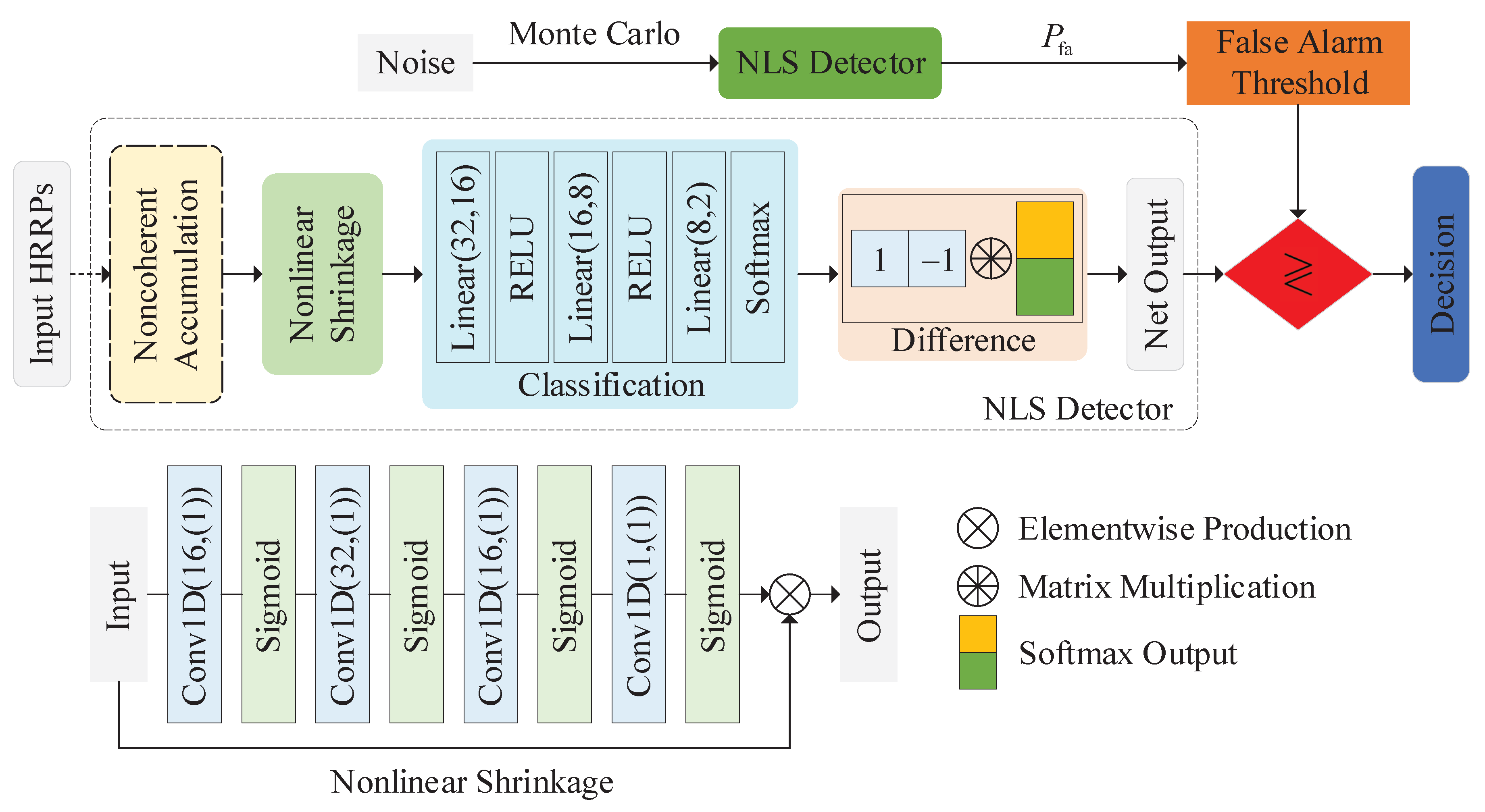
In traditional RST detectors, noise suppression is an efficient way to improve the detection performance. Each of the range bins in the HRRP is treated independently. Range bins are divided into two types: target occupied and noise occupied, and the former are kept for energy integration while the latter are discarded. The MCOM detector in [10] designs a nonlinear shrinkage mapping function for noise suppression and achieves a marked improvement in detection performance, especially for sparse targets. In this subsection, an NLS detector referring to the traditional MCOM detector is proposed. An NLS module is designed to learn a data-adaptive nonlinear shrinkage function, realizing the optimization of the manually designed function in MCOM. The NLS detector takes each of the range bins in the HRRP as an independent low-level feature element. The overall structure of the NLS detector is shown in Figure 2, and the detailed configuration of the network structure is given in Table 1.
The NLS detector takes either a single HRRP or double HRRPs as the network input. The traditional noncoherent accumulation module (labeled with long dash short dash) is specific for the preprocessing of the input of double HRRPs. The following nonlinear shrinkage module learns a data-adaptive shrinkage function to achieve noise suppression for HRRP. The denoised HRRP is fed into a classifier to realize the classification of the input HRRP. The classification output is combined with a difference module, resulting in a scalar output for control of the false alarm rate. The details of the net modules are described as follows:
(1) Noncoherent accumulation: In traditional detectors with double HRRPs as input, the accumulation between HRRPs is beneficial to improving the SNR. The noncoherent accumulation is given as
x nca i   =   | x 1 i |   +   | x 2 i | , i = 1 , , L
where i is the index of the range bin in the HRRP and L is the total number of range bins of a windowed HRRP. x nca is the accumulated result, while x 1 and x 2 are the first and the second of the double HRRPs. | · | indicates the amplitude of the complex data.
In the proposed NLS detector, it is used as the preprocessor to make double HRRPs into a single SNR-improved HRRP.
(2) Nonlinear shrinkage: Nonlinear shrinkage mapping is an efficient way to suppress the noise in the input HRRP when the RST is sparsely distributed [10]. The mapping function is expressed as
y nls = ρ ( x ) · x
where x is a positive number, corresponding to the magnitude of the range bin, and ρ ( x ) is the NLS ratio, which satisfies the following properties:
ρ ( x ) [ 0 , 1 ] , x [ 0 , ) ρ ( x 1 ) ρ ( x 2 ) , when x 1 x 2 lim x 0 + ρ ( x ) = 0 lim x ρ ( x ) = 1
The ratio is calculated based on the input magnitude, according to the given NLS function. The ratio is between 0 and 1 and increases monotonically with the inputted magnitude. Therefore, range bins with large magnitude tend to be kept, and those of small magnitude will be suppressed. In other words, range bins of strong scatterers are kept and those of noise only are discarded, achieving noise reduction. However, the manually designed NLS function is not data adaptive and has limited performance.
Therefore, in the proposed NLS detector, a module based on the convolution structure is proposed for optimization. The structure of the NLS module is shown in the bottom left of Figure 2. In (5), the output NLS ratio ρ ( x ) is determined on a single input value x. Thus, the used convolution layers in the designed module are with a kernel size of 1. It ensures that range bins are treated independently but share the same mapping function. The used activation is “sigmoid” to limit the output ratio within 0 and 1. Multiple convolution layers are concatenated to improve the nonlinear capability. The last layer is with an output channel of 1 to recover the dimension of the NLS ratio. Range bins in the input HRRP are multiplied by the NLS ratio element-wise, forming a denoised output.
(3) Classification module: The classification module consists of several concatenated fully connected layers. The final layer is an activation function of “softmax” with an expression given below:
softmax ( x i ) = exp ( x i ) j = 1 J exp ( x j )
where x = [ x 1 , , x J ] T , i , j { 1 , , J } is an input vector.
The classification module treats the denoised HRRP as a vector in the L-dimensional feature space. Each of the range bins in the denoised HRRP is a low-level feature element. The first two layers serve to enhance the nonlinearity of the module while gradually reducing the output dimension to mitigate computational complexity. However, the output dimension of the final layer needs to be 2, corresponding to the detection result. The outcome after the “softmax” function represents the confidence level for binary classification and is expressed as
P 1 P 0 = F classifier ( W c , x )
where P 1 and P 0 correspond to the confidence of the target present and absence respectively, and P 1 + P 0 = 1 . F classifier ( W c , x ) is an abstract representation of the classification process, W c is the used weight and x here corresponds to the denoised HRRP after NLS module.
(4) Difference module: The traditional classification network is trained with a loss function of cross-entropy and one-hot encoded labels. To make it false alarm controllable, a difference module is introduced in the NLS detector. Based on the difference module, the difference in confidence of binary classification is obtained, which is expressed as
η = 1 1 P 1 P 0 = P 1 P 0
The output is made scalar, and the NLS detector is trained with a loss function of mean square error. The difference in confidence ranges from −1 to 1, and thus, the label is 1 for target present and −1 for target absence.
The net output η in (9) is used as the detection statistic of the NLS detector. Based on Monte Carlo simulation, a threshold T P fa is determined according to the required false alarm rate P fa . For the NLS detector, the detection result is expressed as
η H 1 H 0 T P fa

2.2.2. Deep Detector via Feature Cross-Weighting

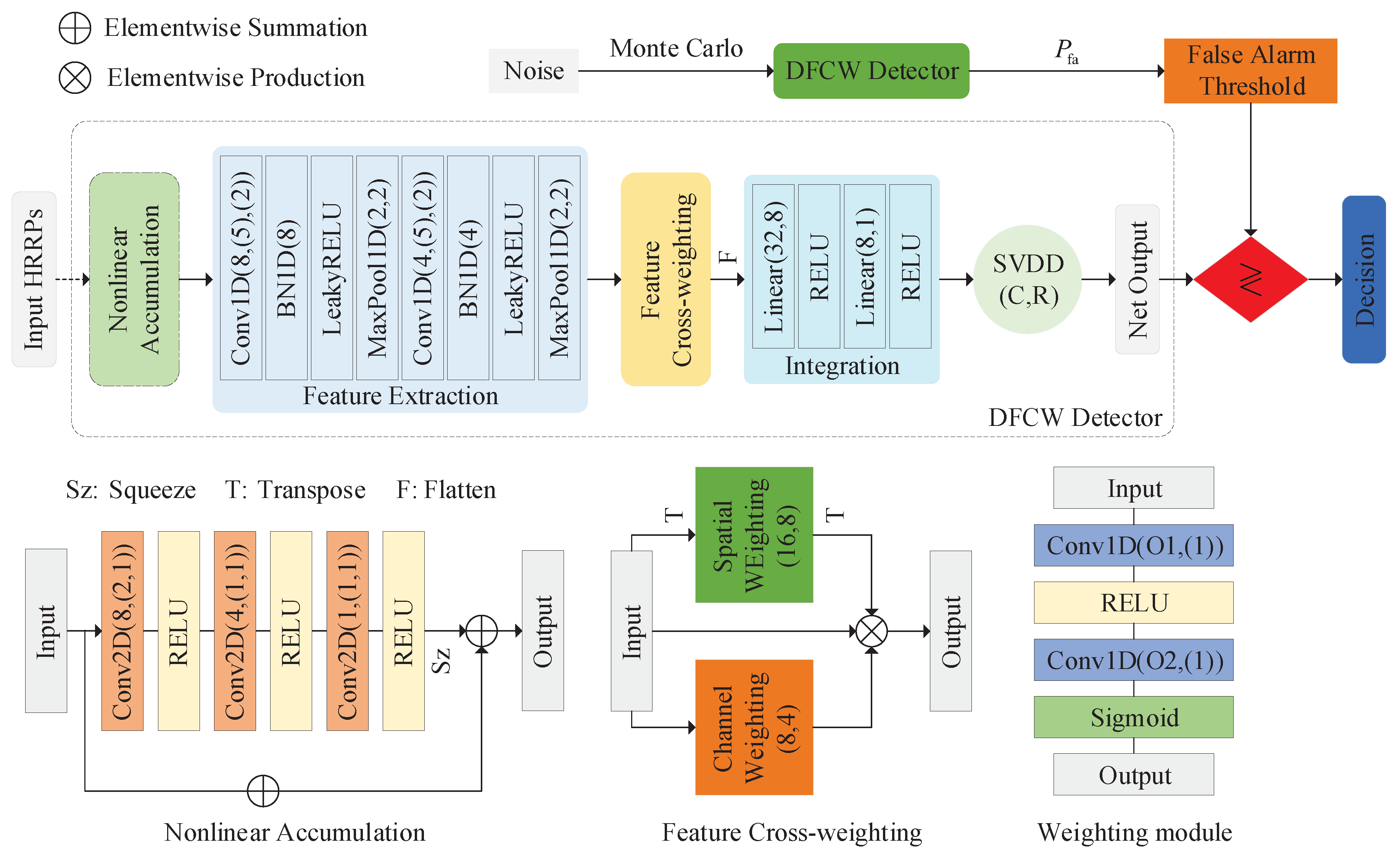
The convolution structure enables the network a good feature extraction capability, of which the extracted features can be precise but usually abstract. Therefore, different from the NLS detector above, which treats the HRRP as a low-level feature vector, a DFCW detector taking advantage of feature extraction is proposed in this subsection. In the proposed DFCW detector, based on the input HRRPs, high-level abstract features are first extracted. A weighting module is used for important feature elements exploitation, and target detection is realized based on the SVDD. The overall structure of the proposed DFWC detector is shown in Figure 3, and the detailed configuration of the network structure is given in Table 2.
The DFCW detector takes either a single HRRP or double HRRPs as network input. For the input of double HRRPs, a nonlinear accumulation module is designed to transform the double HRRPs into an optimized single HRRP. A feature extraction module is introduced, and the high-level feature map of the HRRP is obtained. The following feature cross-weighting module performs element-wise feature weighting in the obtained feature map. The weighted feature map is then integrated using an integration module and results in a scalar statistical feature, which is used for the classification of target and noise based on the SVDD. The details of the net modules are described as follows:
(1) Nonlinear accumulation: In traditional noncoherent accumulation (4), linear summation is applied to the magnitude of each of the range bins in the double HRRPs. However, the accumulation gain is limited. Therefore, a nonlinear accumulation module is developed for optimization of the noncoherent accumulation. The structure of the nonlinear accumulation module is shown in the bottom left of Figure 3.
The two HRRPs are arranged in row-wise, forming a 2 × L input plane. In the designed module, the noncoherent accumulation acts as the skip connection. The first 2D convolution layer is with a kernel size of ( H , W ) = ( 2 , 1 ) . The two following 2D convolution layers are with a kernel size of ( H , W ) = ( 1 , 1 ) . Range bins in the same HRRP are processed independently but identically. Nonlinear addition is performed between range bins from different HRRPs. The nonlinear accumulation is expressed as
x nla i = 1 x i + F nla ( x i , W ) , i = 1 , , L
where i is the index of the range bin and 1 = [ 1 , 1 ] . The x i = [ | x 1 i | , | x 2 i | ] T is the magnitude of range bins from two HRRPs and F nla ( x i , W ) is the residual function output.
(2) Feature extraction: The feature extraction module is used to generate a high-level feature map of the accumulated HRRP.
The used 1D convolution layers are with a kernel size of 5, and local features are extracted. The max pooling layers are with a kernel size of 2, and the redundancy of the adjacent local features is reduced. Unlike the low-level features in the NLS detector, the obtained high-order features in this module are usually concise but abstract.
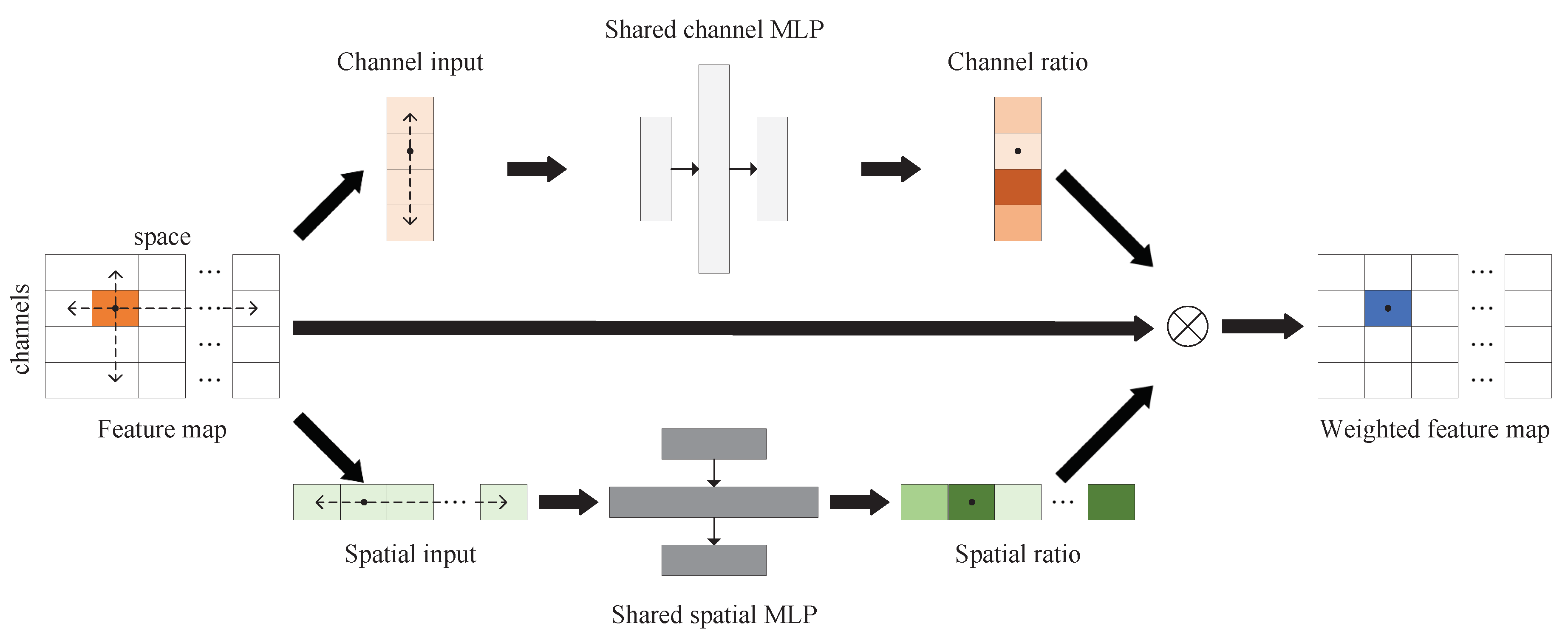
(3) Feature cross-weighting: The output of the feature extraction module is a 2D feature map composed of channel and spatial information. However, each element in the feature map is of a different importance to target detection. Therefore, a module is developed for feature weighting. For each element in the feature map, it is cross-weighted, considering the channel and spatial information jointly. The diagram of feature cross-weighting is shown in Figure 4.
The weighting module in Figure 3 is the shared structure of channel weighting and spatial weighting in the feature cross-weighting module. In the feature map, the spatial dimension is arranged in a row and the channel dimension is arranged in a column, as shown in Figure 4. The feature map is given as
Φ = ϕ 11 ϕ 1 j ϕ 1 J ϕ i 1 ϕ i j ϕ i J ϕ I 1 ϕ I j ϕ I J = [ c 1 , , c j , , c J ] = [ r 1 r i r I ]
where c j = [ ϕ 1 j , , ϕ i j , , ϕ I j ] T , j = 1 , , J represents the j-th column of the feature map. r i = [ ϕ i 1 , , ϕ i j , , ϕ i J ] , i = 1 , , I is the i-th row of the feature map.
The kernel size of 1D convolution in the weighting module is 1. Therefore, each of the columns is processed independently but identically, which is represented by a shared channel multilayer perceptron (MLP). Each of the rows is treated in the same way, using a shared spatial MLP. The channel weighting and spatial weighting are expressed as
c ^ j = F CMLP ( c j ) ,   j = 1 ,   ,   J r ^ i = F SMLP ( r i ) ,   i = 1 ,   ,   I
where F CMLP is the abstract function of the shared channel MLP and F SMLP is the abstract function for the shared spatial MLP. For the input 2D feature map, the channel weighting result and the spatial weighting result are represented as
Φ CW = [ c ^ 1 , , c ^ J ] = α 11 α 1 J α I 1 α I J Φ SW = r ^ 1 r ^ I = β 11 β 1 J β I 1 β I J
where Φ CW and Φ SW are the channel weighting and spatial weighting results of the feature map, respectively. Each element in the weighting matrix is limited from 0 to 1 by the “Sigmoid” function.
A joint channel-spatial weighting is obtained, which is expressed as the production of channel and spatial coefficients:
Φ CSW = Φ CW · Φ SW = α 11 β 11 α 1 J β 1 J α I 1 β I 1 α I J β I J
For each element in the feature map, a joint channel-spatial weighting is performed, and the weighting coefficient is the production of channel and spatial coefficients. The weighted feature map is given as
Φ ˜ = Φ CSW · Φ
In the developed feature cross-weighting module, all elements in the feature map share a weighting function, and the weighting coefficient is calculated based on the joint channel-spatial information. The effective feature elements are assigned with a larger weight and ineffective feature elements are assigned with a smaller feature.
(4) Integration module: The weighted feature map is flattened and fed into the integration module. The integration module consists of two fully connected layers with an activation function of “RELU” for nonlinearity. The output of the second layer is with a single neuron. The feature map is integrated into a scalar statistical feature, which is expressed as
y INT = F INT ( Φ ˜ )
where F INT is the abstract function of the integration module.
(5) SVDD module: The integration result of the feature map is not suitable for training if used as the direct output of network. Therefore, the SVDD is introduced and the target detection is regarded as a problem of anomaly detection.
The SVDD establishes a hyper-sphere to separate two types of data and has been introduced to HRRP recognition in [29]. Based on the integration result of the feature map, the SVDD is formulated as
y SVDD = tanh { ( ξ C ) 2 R 2 }
where tanh ( x ) = exp ( x ) exp ( x ) exp ( x ) + exp ( x ) , C and R are the hyper-sphere center and radius. The labels for target and noise are 1 and −1, respectively. Therefore, target detection based on the SVDD is shown in Figure 5.
The center and radius in SVDD divide the feasible region into detected and undetected regions. Based on the output statistical feature, noise in the undetected region and the target in the detected region are the desired results, and the opposite is undesirable.
For the proposed DFCW detector, the SVDD output is used as the detection statistic, namely ξ = y SVDD . The detection result is expressed as
ξ H 1 H 0 T P fa

3. Experiments and Results

In this section, four experiments are conducted to analyze the effectiveness of the two proposed network detectors. The organization of the four experiments is shown in Table 3.
The first three experiments are ablation experiments, which are used to verify the contribution of the designed modules to the detection performance of the proposed network detectors. The final experiment is the performance comparison with reference detectors to verify the effectiveness of the proposed detectors.

3.1. Dataset Description

The received HRRPs are used in this work for the detection of an RST, and only the magnitude of HRRPs is considered. Two datasets are generated for tje evaluation of the performance of RST detectors. The first dataset is a simulated dataset and the second dataset is a measured dataset based on real radar data. As illustrated in (3), target detection is considered in scenarios using a single HRRP and double HRRPs. Therefore, each of the datasets are further divided into the single-HRRP dataset and double-HRRP dataset.
For the generation of datasets, the influence of the target spread characteristic on detector performance is considered, as described in [36], of which the target spread characteristic is modeled as the sparseness of HRRP. Therefore, the defined quantitative measurement of sparseness in [36] is introduced to characterize the datasets and is expressed as
sparseness ( x ) = 1 N i x i 4 ( i x i 2 ) 2 1 N 1
where the sparseness of an HRRP is in the range of 0 to 1. An HRRP with a sparseness of 0 indicates all range bins in the window are of equal magnitude. It is usually the worst case. There are not strong scatterers in the RST, and detection performance is poor. An HRRP with a sparseness of 1 indicates that only a single range bin is of non-zero magnitude. Target energy is concentrated, and the RST becomes a point target. With the HRRP is a fixed size, the detection of an RST is easier with the increase in HRRP sparseness.
The signal energy-to-noise ratio (ENR) in [37] is introduced to describe the signal intensity for radar target detection, which is given as
ENR = l = 1 L s l 2 1 L l = 1 L n l 2
where the numerator is the energy of the signal, and the denominator is the power of the noise. The ENR is a preferred definition for analyzing radar target detection performance, and the relationship between ENR and SNR is ENR = SNR + 10 log 10 ( L ) .

3.1.1. Simulated Dataset

In the simulated dataset, the RST is represented by a window of continuous range bins with length L = 32 . The magnitude of a single range bin follows one of the three uniform distributions, which are U ( 0.4 , 1.0 ) , U ( 0 , 0.6 ) and U ( 0 , 0.1 ) , corresponding to the strong, moderate and weak scatterers, respectively. The phase of range bins follows U ( 0 , 2 π ) . The magnitude and phase of range bins are set independently.
The simulated dataset is with a sparseness range of 0.1 to 0.5 and it is divided into two parts.
The first part is used for training the network. The sparseness is continuously distributed. There are 24,000 different target HRRPs, and they are energy-normalized. Based on these noiseless HRRPs, noise is added to form noisy HRRPs. In this work, the added noise in a single range bin is assumed to be complex Gaussian noise with unit power, i.e., CN ( 0 , 1 ) , and noise in different range bins is independent and identically distributed. A total of 288,000 noisy HRRPs are generated, and the formed ENRs range from 7 dB to 18 dB . The same number of HRRPs consisting only of noise is generated for class balance. Therefore, a total of 576,000 input HRRPs are available for network training.
The second part is used for the performance evaluation of detectors. The sparseness is sampled with an interval of 0.05 in [ 0.1 , 0.5 ] , and there are nine samples of sparseness in total. For each sampled sparseness, 10 different noiseless HRRPs are generated. Therefore, a total of 90 target HRRPs are generated. The detection performance of a detector is obtained using the Monte Carlo simulation method. The number of Monte Carlo simulations is 2000. In other words, for each of the 90 target HRRPs, 2000 noisy samples are generated for a single ENR. The sampled ENR is from 0 to 18 dB with an interval of 1 dB . Thus, a total of 3,420,000 noisy HRRPs of targets are obtained. In addition, 5000 HRRPs consisting only of noise are generated to calculate the required false alarm threshold. Therefore, the number of input HRRPs for evaluation is 3,425,000.
The generated dataset above is for the single-HRRP detection case. In the double-HRRP detection case, for each input sample of the target, an identical pair of noiseless HRRPs are generated, and they are added with independent noise. For each input sample of noise, a pair of HRRPs consisting only of independent noise is generated.
Examples of the simulated dataset are shown in Figure 6.

3.1.2. Measured Dataset

Experimental data are used in this work. The monitored target is a satellite, the and data are collected by the real radar. The experimental data are with high SNR and are regarded as noiseless data. The target is located in a windowed HRRP of length L = 32 , and a total of 312 HRRPs are available.
The sparseness of the obtained HRRPs ranges from 0.1 to 0.35. They are divided into two parts, 292 HRRPs for constructing the training set and 20 HRRPs for constructing the evaluation set.
Data enhancement is used while generating the training set. Flip operations on the left and right side, cyclic shift and noise addition are used for each of the 292 HRRPs. The flip operation doubles the number of HRRPs, and each of these HRRPs performs cyclic shift four times independently. Therefore, 2336 noiseless HRRPs are generated. The ENR of the training set ranges from 7 to 18 dB , and for a single ENR, each noiseless HRRP performs noise addition eight times independently. Thus, a total number of 2336 × 8 × 12 = 224,256 noisy target HRRPs are generated. For class balance while training, the same number of HRRPs consisting only of noise is generated.
To construct the evaluation set, each of the 20 HRRPs generates 2000 noisy HRRPs for a single ENR. The formed ENR ranges from 0 to 18 dB . A total of 760,000 noisy target HRRPs are generated, and 5000 HRRPs of noise are also generated.
For the measured dataset in the double-HRRP case, it is constructed in the same way as the simulated dataset.
Examples of the measured dataset are shown in Figure 7.
Two examples of experimental HRRPs are shown in Figure 7a. In Figure 7b, the obtained HRRPs from the satellite are of low sparseness. The sparseness is non-uniformly distributed, and most are around the range of 0.1 to 0.2. In Figure 7c, the 292 HRRPs are sorted in order of sparseness. The 20 HRRPs for evaluation are evenly sampled from the sorted HRRPs, and the rest are for training.

3.2. Experimental Platform and Training Details

The mentioned network models in this work are implemented using PyTorch. Training and evaluation are complemented on the Intel(R) Core(TM) i7-10700F CPU with 32 GB RAM and GeForce GTX 1660 SUPER with 6 GB graphics memory. The batch size is set as 128, and the training epoch is 50 for all models. For the two proposed detectors, they are optimized with an Adam optimizer with the initialized learning rate of 0.001, and the learning rate is decayed by a factor of 0.1 at epochs 35 and 45. The hyper-parameters of the DFCW detector are set as C = 0.0 and R = 0.5 . For the referenced CNN-LSTM detector, the settings are kept as those originally provided in [29].
In the network training process, the training set in each of the generated datasets is further divided into two parts with a ratio of 8:2 for training and validation, respectively.

3.3. Evaluation Indicators

For radar detection, the detection performance is evaluated with the probability of detecting a target under the limitation of a fixed false alarm rate.
The false alarm rate is given as
P fa = x : L ( x ) > T thr p ( x ; H 0 ) d x
where x is the input signal, L ( x ) is the detection statistic, and T thr is the selected detection threshold. p ( x ; H 0 ) is the probability density function (PDF) of x in the case of H 0 . Usually, the false alarm rate P fa is set to a required value, i.e., P fa = α , and the detection threshold is calculated based on the required P fa .
The detection probability is given as
P d = x : L ( x ) > T thr p ( x ; H 1 ) d x
where p ( x ; H 1 ) is the PDF of x in the case of H 1 . The P d is related to both the T thr and the signal intensity, namely ENR.
However, because of the nonlinearity of the network, theoretical expressions of the detection statistics, i.e., η and ξ , are not available. Therefore, in this work, Monte Carlo simulations are conducted based on the generated datasets to obtain the numerical solutions of P fa and P d . Taking the performance analysis of the NLS detector on the simulated dataset as an example, the calculations of P fa and P d are as follows:
  • Based on the evaluation set, 5000 samples for η are obtained and sorted in descending order, i.e., η H 0 1 > η H 0 2 > > η H 0 5000 .
  • The false alarm rate is set to the desired value, i.e., P fa = 1 × 10 3 .
  • The detection threshold T thr is set to a value close to but less than η H 0 5 , so that the number of false alarms is 5, corresponding to P fa = 5 / 5000 = 1 × 10 3 .
  • For one of the 90 target HRRPs, at each ENR, 2000 samples for η are obtained, i.e., { η H 1 1 , , η H 1 2000 } . The detection probability is calculated as P d = 1 2000 i = 1 2000 ( η H 1 i > T thr ) .
In this way, a performance curve of the detection probability via ENR with the desired false alarm rate is obtained.
Therefore, the first used indicator for evaluation is the detection performance curve. In this work, the desired false alarm rate is set as P fa = 1 × 10 3 . The evaluation sets in the simulated dataset and measured dataset contain 90 and 20 independent target HRRPs, respectively. Thus, for each of the datasets, an averaged performance curve is obtained and used as the indicator.
One more indicator used in this work is the global detection probability. It is an overall metric and is used to quantify the detection probability on the entire evaluation set, which is formulated as
P global = N cdt N t
where the N cdt is the number of correct detections of the target in the evaluation set, and N t is the total number of target samples in the evaluation set. Taking the simulated dataset as an example, N t = 19 × 2000 × 90 and N cdt are the number of detection statistic samples greater than T thr .

3.4. Experimental Results

For performance comparison, based on the evaluation indicators, the experimental results are organized according to the used dataset and the number of used HRRPs, i.e., single HRRP detection on the simulated dataset, double HRRP detection on the simulated dataset, single HRRP detection on the measured dataset and double HRRP detection on the measured dataset.

3.4.1. Experimental Results of the NLS Module

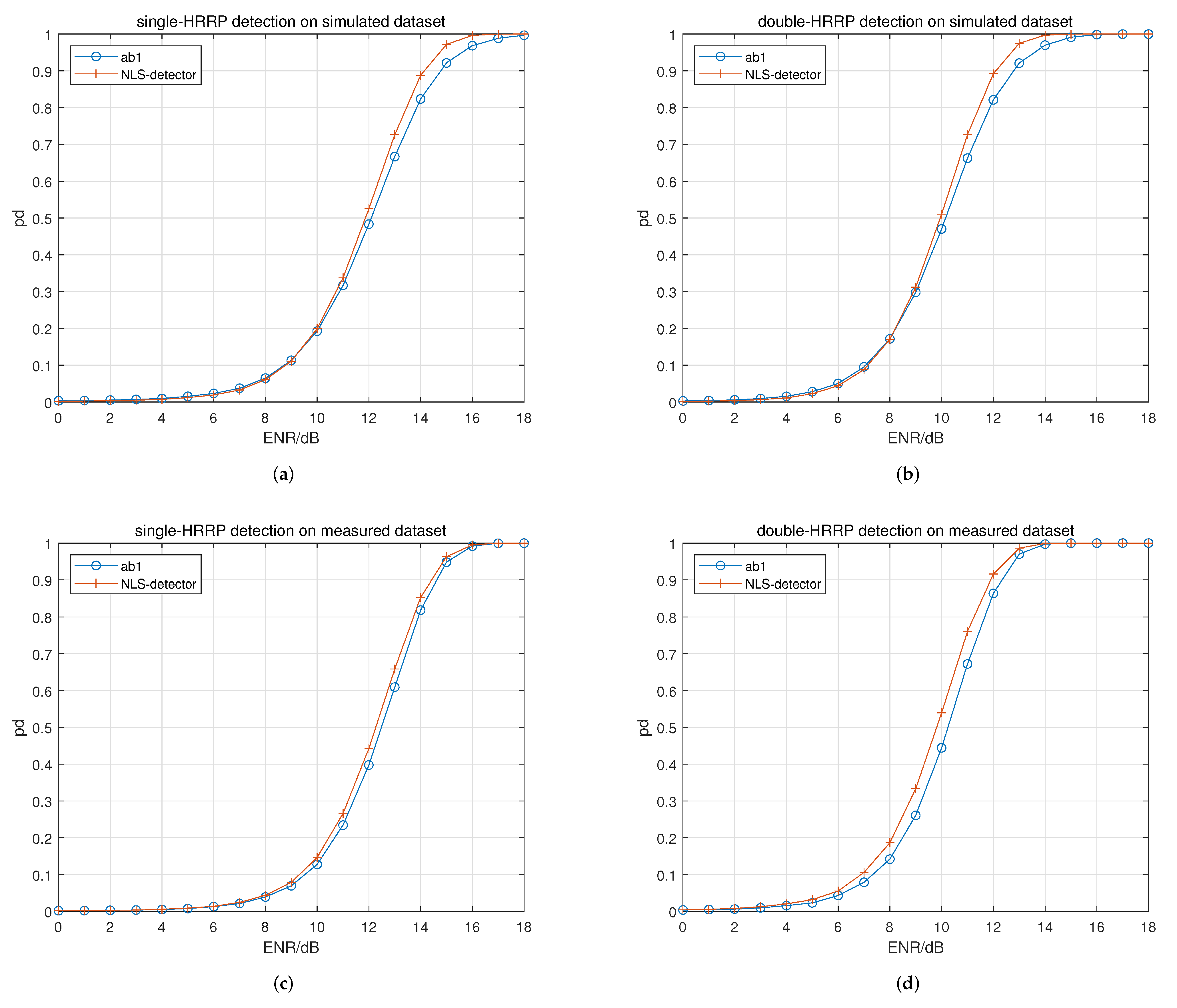
In experiment 1, the effects of the NLS module on the performance of the proposed NLS detector in different detection scenarios are studied. A model removing the NLS module is used as the baseline model for comparison. The results are given in Figure 8 and Table 4.
In Figure 8a,b where the simulated dataset is used, the NLS detector, compared with the baseline model, shows a significant improvement on the detection performance under high ENRs. In Figure 8c,d where the measured dataset is used, the performance curve of the proposed NLS detector moves to the left at different degrees compared to that of the baseline model.
For the quantitative results in Table 4, it can be seen that the P global values in four scenarios are all improved. The improvements in P global from left to right are 1.35%, 1.30%, 1.15%, and 2.26%, respectively.

3.4.2. Experimental Results of the Nonlinear Accumulation Module

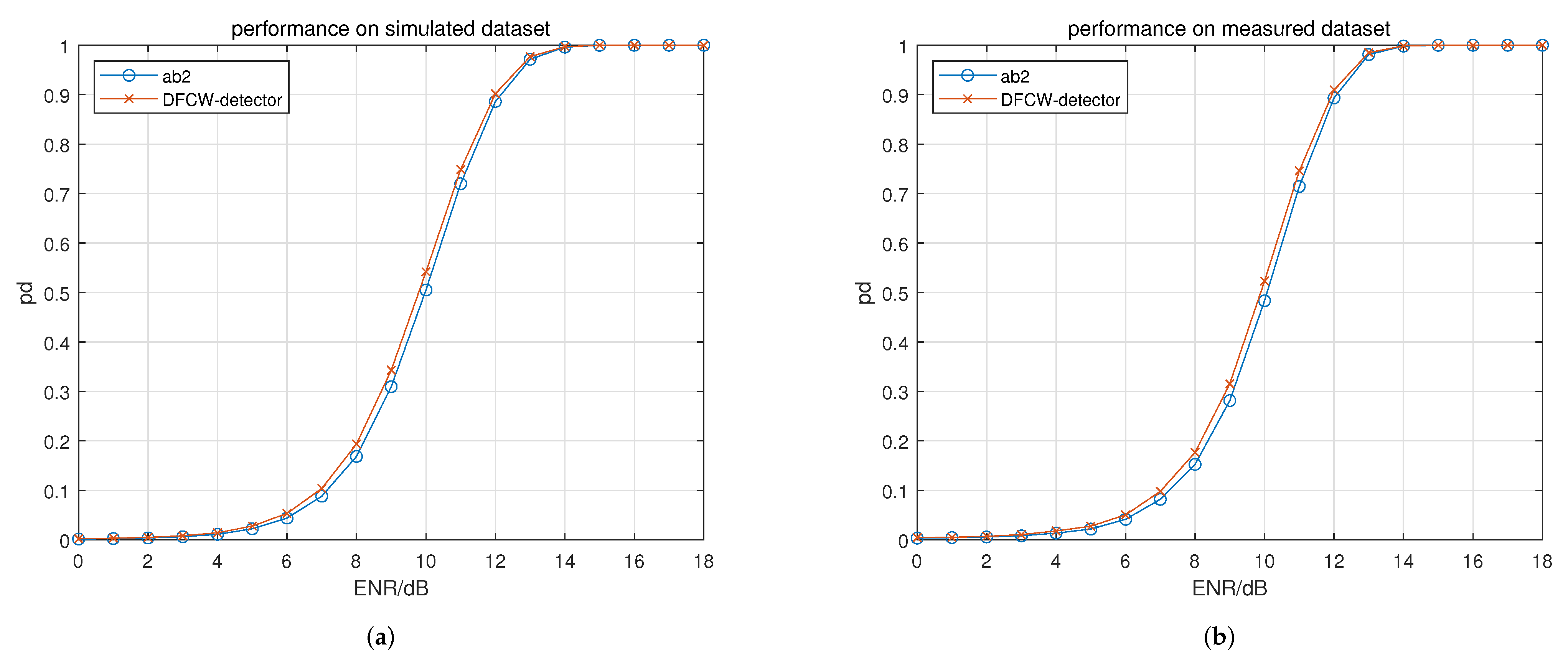
In experiment 2, for the proposed DFCW detector, the contribution of the nonlinear accumulation module on detection performance is evaluated. The nonlinear accumulation module in the DFCW detector is replaced by a traditional noncoherent accumulation and used as comparison. The experiment is conducted on the double HRRP dataset. The results are shown in Figure 9 and Table 5.
In Figure 9, it can be seen that the nonlinear accumulation module makes the detection performance better on both the simulated and measured datasets.
Based on the obtained P global in Table 5, it can be seen that the P global values are increased by 0.98% and 1.0%, respectively.

3.4.3. Experimental Results of the Feature Cross-Weighting Module

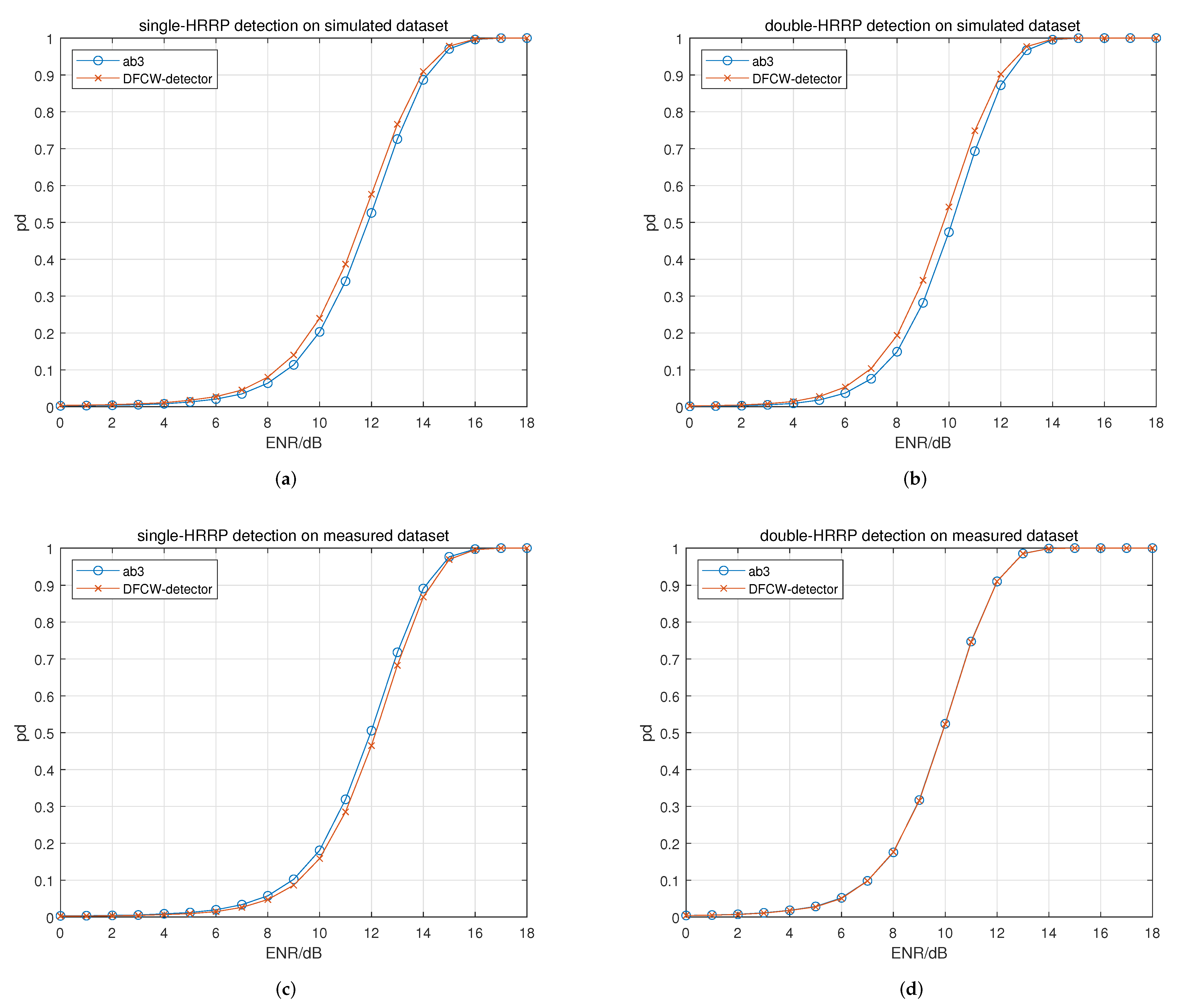
In experiment 3, the effect of the feature cross-weighting module on the detection performance is evaluated. The DFCW detector removing the feature cross-weighting module is used as comparison. The results are given in Figure 10 and Table 6.
Figure 10a,b represent the single-HRRP and double-HRRP detection performance on the simulated dataset. It can be seen that the performance is improved by using the feature cross-weighting module. Figure 10c,d show the results of the measured dataset. However, with the feature cross-weighting module, the performance is decreased in the single HRRP detection scenario and is basically unchanged in the double-HRRP detection scenarios.
From Table 6, the differences in P global from left to right are 1.48%, 1.78%, −1.11% and −0.04%, respectively. In other words, the effect of the feature cross-weighting module on detection performance changes with the used dataset.

3.4.4. Experimental Results of Performance Comparison

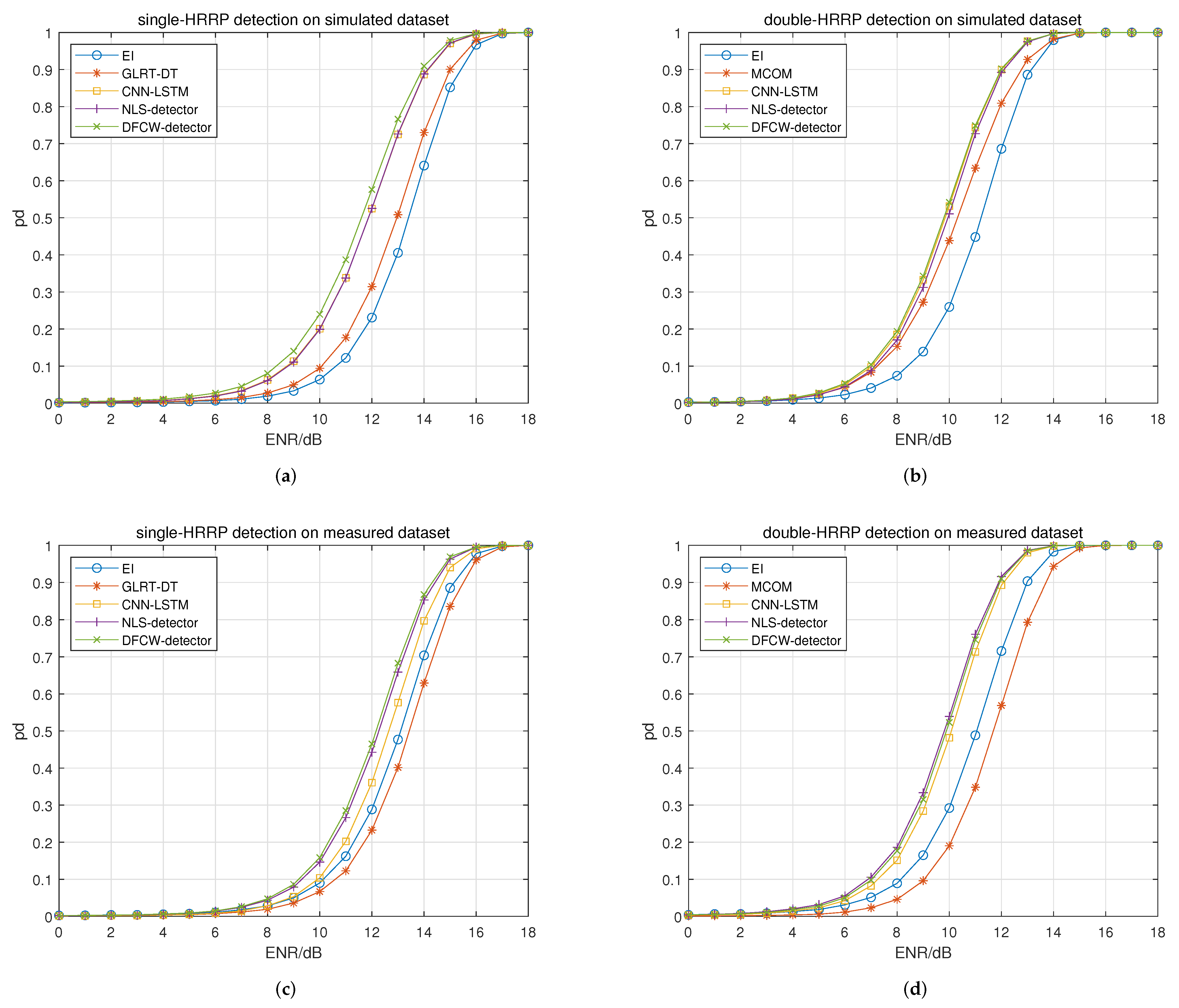
In experiment 4, the effectiveness of the proposed detection networks is verified by performance comparison with traditional and deep learning-based detectors. For the traditional detector, the EI detector [3], GLRT-DT detector [5] and MCOM detector [10] are used. For the deep learning-based detector, the CNN-LSTM detector [29] is used. Experimental results are shown in Figure 11 and Table 7.
Figure 11a shows the single-HRRP detection performance on the simulated dataset. It can be seen that the deep learning-based detectors are much better than traditional detectors. For the deep learning-based detector, the DFCW detector performs better than the other two detectors. The performance of the CNN-LSTM detector and the NLS detector is basically the same. For all detectors, the detection performance in descending order is DFCW detector, CNN-LSTM detector, NLS detector, GLRT-DT detector and EI detector.
Figure 11b shows the double-HRRP detection performance on the simulated dataset. It can be seen that although the deep learning-based detectors are better than traditional detectors, the performance gap between traditional detectors and deep learning-based detectors is narrowed. The MCOM detector approaches deep learning-based detectors at low ENRs but suffers performance degradation compared with that of deep learning-based detectors at high ENRs. For the deep learning-based detectors, the three detectors are close to each other. For all detectors, the detection performance in descending order is DFCW detector, CNN-LSTM detector, NLS detector, MCOM detector and EI detector.
Figure 11c shows the single-HRRP detection performance on the measured dataset. It can be seen that the performance gap is further narrowed. For deep learning-based detectors, the DFCW detector and the NLS detector are comparable, and both are better than the CNN-LSTM detector. For all detectors, the detection performance in descending order is DFCW detector, NLS detector, CNN-LSTM detector, EI detector and GLRT-DT detector.
Figure 11d shows the double-HRRP detection performance on the measured dataset. It can be seen that the performance gap between traditional detectors and deep learning-based detectors becomes wider. For deep learning-based detectors, the two proposed detectors are better than the CNN-LSTM detector, but the performance improvement is decreased compared with the single-HRRP detection scenario. For all detectors, the detection performance in descending order is NLS detector, DFCW detector, CNN-LSTM detector, EI detector and MCOM detector, respectively.

4. Discussion

4.1. Analysis of NLS Module

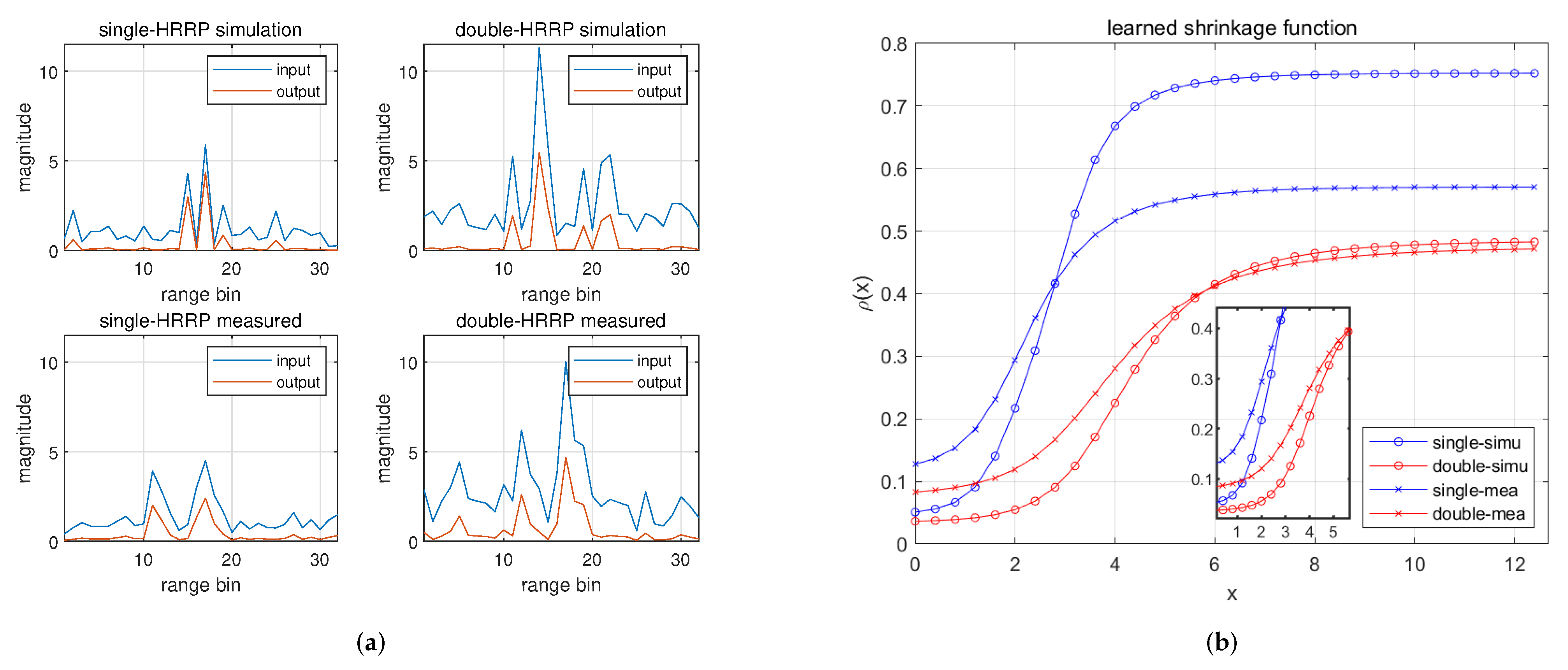
Based on the results of experiment 1, it can be seen that the NLS module behaves differently on different datasets. For detailed analysis, the outputs and the learned nonlinear shrinkage functions of the NLS module in four detection scenarios are shown in Figure 12.
In Figure 12a, the inputs and outputs of the NLS module are shown. The two subplots at the top are based on the simulated dataset, and the two at the bottom are based on the measured dataset. The two subplots on the left are based on a single HRRP, and the two on the right are based on double HRRPs. Overall, it can be seen that the smaller the magnitude of a single range bin, the stronger the extent of suppression. In Figure 12b, the learned nonlinear shrinkage functions are shown. It can be seen that the nonlinear shrinkage functions are different with each other and are adaptive to the specific dataset. In the double-HRRP scenarios, the two HRRPs are noncoherently accumulated, and the magnitude is much larger than that of single-HRRP scenarios, as shown in Figure 12a. In Figure 12b, the learned nonlinear shrinkage curves for the double-HRRP case are shifted to the right on the x-axis, corresponding to larger input. The difference in the sparseness of datasets also affects the learned nonlinear shrinkage functions. The measured dataset has a much lower sparseness than the simulated dataset, and the unsaturated intervals of curves of the measured dataset are to the left of that of the simulated dataset, as shown in the zoom plot.

4.2. Analysis of Nonlinear Accumulation Module

In experiment 2, the nonlinear accumulation shows a positive contribution on detection performance. To further analyze the effect of the nonlinear accumulation module, the outputs of this module are given in Figure 13.
Figure 13a,b show the outputs of the nonlinear accumulation module trained on the simulated and measured dataset, respectively. The top subplot corresponds to a noisy target HRRP with an ENR of 18 dB, and the bottom subplot corresponds to a noise input. It can be seen that the residual output has a small value on the range bin where the output magnitude of the noncoherent accumulation is large. Once the noncoherent accumulation output is larger than a certain value, the residual output reaches zero. Therefore, in the region where the noncoherent accumulation output is smaller than a certain value, the output is compensated by the residual output, making the magnitude fluctuation flattened, as shown in the nonlinear accumulation output. On the contrary, the regions where the noncoherent accumulation output is large are kept unchanged, and these regions tend to be range bins of strong scatterers. This characteristic of the nonlinear accumulation output could be a reason for the improvement of detection performance.

4.3. Analysis of Feature Cross-Weighting Module

The feature cross-weighting module is based on the extracted high-level feature map of the HRRP, and the reasonability of the weighting coefficients will influence the detection performance. From the results, the feature cross-weighting module performs well in the double-HRRP detection scenario of the simulated dataset but poorly in the single-HRRP detection scenario of the measured dataset. Therefore, in this subsection, the effectiveness of the module is analyzed, considering the difference in the detection scenarios.
The sparseness of the simulated dataset ranges from 0.1 to 0.5, which is higher than that of the measured dataset (0.1 to 0.35). For an RST, the higher the sparseness of the target HRRP, the fewer the number of scatterers and the stronger the amplitude of the scatterers. Thus, in this case, it is easier to distinguish target from noise. Using double HRRPs for detection provides more target information. Therefore, it is reasonable to assume that the higher the sparseness of dataset and the more HRRP used, the easier it is for the module to obtain suitable weighting coefficients for the feature map. The performance gain of the feature cross-weighting module in descending order is 1.78% > 1.48% > −0.04% > −1.11%, corresponding to the four scenarios from the simulated dataset to the measured dataset and from double-HRRP detection to single-HRRP detection as expected.
Specifically, for double-HRRP detection on the measured dataset, the low sparseness poses challenges in calculating reasonable weighting coefficients, yet leveraging double HRRPs can compensate for this limitation. Thus, it may explain the result in Figure 10d, where the influence of the two factors appears to be evenly balanced. The same is also applicable for the other three scenarios in Figure 10.

4.4. Analysis of Detection Performance

Overall, the detection performance is related to the detection scenarios. For the two datasets in this work, the transition from the measured dataset to the simulated dataset results in the increase in sparseness and enhances the detectors’ performance. Therefore, the performance curves shift to the right from Figure 11a to Figure 11c and from Figure 11b to Figure 11d. Increasing the number of used HRRPs results in performance improvement, too. Thus, the performance curves shift to the left from Figure 11a to Figure 11b and from Figure 11c to Figure 11d.
Although the trend remains consistent, variations in detection performance still exist among different types of detectors. Based on the experimental results, the performance comparison of different detectors is given as follows.
For traditional detectors, the EI detector is the only one that is not affected by the sparseness of HRRPs. Therefore, the EI detector in the measured dataset obtains better performance compared with the other traditional detectors. However, in the simulated dataset, the GLRT-DT and the MCOM detectors benefit from the increased sparseness and are superior to the EI detector. The MCOM detector requires at least two HRRPs to perform target detection and is better than the GLRT-DT detector in the sparse and double-HRRP detection scenario.
For deep learning-based detectors, they consistently outperform traditional detectors in the four detection scenarios. This advantage stems from the network’s capability to learn more efficient representations for distinguishing between targets and noise.
However, discrepancies persist among the three deep learning-based detectors. The NLS detector regards the HRRP as a feature vector and implements traditional signal processing through a network module, ensuring the physical meaning of the module outputs is retained. The CNN-LSTM detector and the DFCW detector are based on the feature map of the HRRP. The LSTM structure is introduced to explore the relationship between spatial features. However, in the initial HRRP, scatterers of an RST exhibit relative independence, resulting in a weak spatial correlation. Therefore, the LSTM module does not ensure performance improvement. The feature cross-weighting module in the DFCW detector, considering the independence of spatial features, treats each element in the feature map independently but identically and calculates a weighting coefficient to represent the importance of each feature element.
A detailed performance comparison of deep learning-based detectors is shown in Table 8, which is given as the difference in P global .
The results presented in the table represent the performance enhancements achieved by the two proposed network detectors with the performance of the CNN-LSTM detector serving as a benchmark. It can be seen that the detection performance of the NLS detector is slightly worse than the referenced CNN-LSTM detector in the simulated dataset, but it is much better in the measured dataset. For the DFCW detector, it outperforms the CNN-LSTM detector in all detection scenarios. Furthermore, the table results can also be analyzed from the following two perspectives:
1. Considering the influence of the sparseness of datasets, the sorted results are expressed as 2.21% > −0.03% and 1.47% > −0.56% for the first line and 2.82% > 1.54% and 1.0% > 0.27% for the second line. In other words, the CNN-LSTM detector suffers much more serious performance degradation when the sparseness of used dataset decreases compared to the NLS detector and the DFCW detector.
2. Considering the influence of the number of used HRRPs, the sorted results are given as −0.03% > −0.56% and 2.21% > 1.47% for the first line and 1.54% > 0.27% and 2.82% > 1.0% for the second line. In other words, the CNN-LSTM detector exhibits a greater performance improvement as the number of used HRRPs increases compared to the NLS detector and the DFCW detector.
Therefore, compared with the CNN-LSTM detector, the two proposed detectors demonstrate enhanced adaptability in challenging scenarios, such as a dataset with low sparseness or detection using a single HRRP. In comparing the two proposed detectors, the DFCW detector performs best in the two detection scenarios on the simulated dataset and the single-HRRP detection scenario on the measured dataset, but the NLS detector achieves the best performance in the double-HRRP detection scenario on the measured dataset.

5. Conclusions

In the HRR, an RST is represented by multiple scatterers, and the dispersed target energy causes a degradation of detection performance. Traditional RST detectors, relying on manually designed test statistics, encounter performance limitations. Therefore, in this work, deep learning is utilized to adaptively design RST detectors, leading to the proposal of two network detectors aimed at enhancing detection performance. The proposed NLS detector treats HRRP as a low-level feature vector and employs a network module to achieve an adaptive design of the traditional nonlinear shrinkage function. The output of the module is a denoised HRRP, which can be used to enhance the detection performance. The proposed DFCW detector takes advantage of the high-level feature map of the HRRP. A feature cross-weighting module is designed in the DFCW detector to achieve element-wise feature weighting and selection based on the extracted feature map. Additionally, for double-HRRP detection, the DFCW detector incorporates a nonlinear accumulation module designed to optimize traditional noncoherent accumulation operations, thereby enhancing target detection performance. Two datasets with different sparseness ranges are generated and utilized to evaluate the performance of detectors. The experimental results demonstrate that deep learning-based detectors can dynamically adjust to the dataset and achieve superior detection performance compared to traditional detectors. In this work, the designed modules utilize convolutional layers with a kernel size of 1 to ensure independent but uniform processing of different spatial features, making a positive overall contribution to detection performance. Compared to the CNN-LSTM detector, the two proposed network detectors show greater adaptability in challenging scenarios. Specifically, the NLS detector performs best in the double-HRRP detection scenario of the measured dataset, and the DFCW detector outperforms in the remaining three scenarios.

Author Contributions

Conceptualization, Y.Y.; methodology, Y.Y.; software, Y.Y.; validation, Y.Y.; formal analysis, Y.Y. and P.P.; investigation, Y.Y. and P.P.; resources, Y.Y. and Z.D.; data curation, Y.Y. and W.H.; writing—original draft preparation, Y.Y.; writing—review and editing, Y.Y., Z.D., P.P. and W.H.; visualization, Y.Y., Z.D., P.P. and W.H.; supervision, Z.D.; project administration, Z.D.; funding acquisition, Z.D. All authors have read and agreed to the published version of the manuscript.

Funding

The research was supported in part by the Science, Technology and Innovation Commission of Shenzhen Municipality under Grant JCYJ20210324120002007, in part by the Science and Technology Planning Project of Key Laboratory of Advanced IntelliSense Technology, Guangdong Science and Technology Department under Grant 2023B1212060024.

Data Availability Statement

The raw data supporting the conclusions of this article will be made available by the authors on request.

Conflicts of Interest

The authors declare no conflicts of interest.

References

  1. Long, T.; Liang, Z.; Liu, Q. Advanced technology of high-resolution radar: Target detection, tracking, imaging, and recognition. Sci. China Inf. Sci. 2019, 62, 40301. [Google Scholar] [CrossRef]
  2. Wang, G.; Wei, Y.; Ding, Z.; You, P.; Liu, S.; Zhang, T. Multi-Dimensional Spread Target Detection with Across Range-Doppler Unit Phenomenon Based on Generalized Radon-Fourier Transform. Remote Sens. 2023, 15, 2158. [Google Scholar] [CrossRef]
  3. Hughes, P. A High-Resolution Radar Detection Strategy. IEEE Trans. Aerosp. Electron. Syst. 1983, AES-19, 663–667. [Google Scholar] [CrossRef]
  4. Jiayun, C.; Xiongjun, F.; Wen, J.; Min, X. Design of high-performance energy integrator detector for wideband radar. J. Syst. Eng. Electron. 2019, 30, 1110–1118. [Google Scholar] [CrossRef]
  5. Long, T.; Zheng, L.; Li, Y.; Yang, X. Improved double threshold detector for spatially distributed target. IEICE Trans. Commun. 2012, 95, 1475–1478. [Google Scholar] [CrossRef]
  6. Ma, T.; Gai, J.; Liang, Z.; Liu, Q.; Liu, H. Weighted Double Threshold Wideband Detector Based on Generalized Likelihood Ratio Test. In Proceedings of the 2021 IEEE International Conference on Signal Processing, Communications and Computing (ICSPCC), Xi’an, China, 17–20 August 2021; pp. 1–4. [Google Scholar] [CrossRef]
  7. Chen, X.; Gai, J.; Liang, Z.; Liu, Q.; Long, T. Adaptive Double Threshold Detection Method for Range-Spread Targets. IEEE Signal Process. Lett. 2022, 29, 254–258. [Google Scholar] [CrossRef]
  8. Gerlach, K.; Steiner, M.; Lin, F. Detection of a spatially distributed target in white noise. IEEE Signal Process. Lett. 1997, 4, 198–200. [Google Scholar] [CrossRef]
  9. Ren, Z.; Yi, W.; Zhao, W.; Kong, L. Range-Spread Target Detection Based on Adaptive Scattering Centers Estimation. IEEE Trans. Geosci. Remote Sens. 2023, 61, 1–14. [Google Scholar] [CrossRef]
  10. Shui, P.L.; Xu, S.W.; Liu, H.W. Range-Spread Target Detection using Consecutive HRRPs. IEEE Trans. Aerosp. Electron. Syst. 2011, 47, 647–665. [Google Scholar] [CrossRef]
  11. Xu, S.W.; Shui, P.L. Range-spread target detection in white Gaussian noise via two-dimensional non-linear shrinkage map and geometric average integration. IET Radar Sonar Navig. 2012, 6, 90–98. [Google Scholar] [CrossRef]
  12. Xu, S.; Shui, P. Range-spread target detection using 2D non-local nonlinear shrinkage map. Signal Process. 2014, 98, 337–343. [Google Scholar] [CrossRef]
  13. Zhang, X.W.; Yang, D.D.; Huang, W.Z.; Guo, J.X.; Hou, Y. Range-spread target detection using the time-frequency feature based on sparse representation. Int. J. Electron. 2018, 105, 1388–1398. [Google Scholar] [CrossRef]
  14. Chen, X.; Hou, K.; Chang, S.; Liu, Q.; Ren, W. Detection of range-spread targets based on order statistics. Digit. Signal Process. 2023, 133, 103803. [Google Scholar] [CrossRef]
  15. Pan, P.; Zhang, Y.; Deng, Z.; Wu, G. Complex-Valued Frequency Estimation Network and Its Applications to Superresolution of Radar Range Profiles. IEEE Trans. Geosci. Remote Sens. 2022, 60, 1–12. [Google Scholar] [CrossRef]
  16. Xu, B.; Chen, B.; Wan, J.; Liu, H.; Jin, L. Target-Aware Recurrent Attentional Network for Radar HRRP Target Recognition. Signal Process. 2019, 155, 268–280. [Google Scholar] [CrossRef]
  17. Gao, C.; Yan, J.; Zhou, S.; Varshney, P.K.; Liu, H. Long short-term memory-based deep recurrent neural networks for target tracking. Inf. Sci. 2019, 502, 279–296. [Google Scholar] [CrossRef]
  18. Wang, C.; Tian, J.; Cao, J.; Wang, X. Deep Learning-Based UAV Detection in Pulse-Doppler Radar. IEEE Trans. Geosci. Remote. Sens. 2022, 60, 1–12. [Google Scholar] [CrossRef]
  19. Liu, N.; Xu, Y.; Tian, Y.; Ma, H.; Wen, S. Background classification method based on deep learning for intelligent automotive radar target detection. Future Gener. Comput. Syst. 2019, 94, 524–535. [Google Scholar] [CrossRef]
  20. Diskin, T.; Beer, Y.; Okun, U.; Wiesel, A. CFARnet: Deep learning for target detection with constant false alarm rate. arXiv 2022, arXiv:2208.02474. [Google Scholar] [CrossRef]
  21. Lin, C.H.; Lin, Y.C.; Bai, Y.; Chung, W.H.; Lee, T.S.; Huttunen, H. DL-CFAR: A Novel CFAR Target Detection Method Based on Deep Learning. In Proceedings of the 2019 IEEE 90th Vehicular Technology Conference (VTC2019-Fall), Honolulu, HI, USA, 22–25 September 2019; pp. 1–6. [Google Scholar] [CrossRef]
  22. Cao, Z.; Fang, W.; Song, Y.; He, L.; Song, C.; Xu, Z. DNN-Based Peak Sequence Classification CFAR Detection Algorithm for High-Resolution FMCW Radar. IEEE Trans. Geosci. Remote Sens. 2022, 60, 1–15. [Google Scholar] [CrossRef]
  23. Jiang, W.; Ren, Y.; Liu, Y.; Leng, J. A method of radar target detection based on convolutional neural network. Neural Comput. Appl. 2021, 33, 9835–9847. [Google Scholar] [CrossRef]
  24. Pérez, R.; Schubert, F.; Rasshofer, R.; Biebl, E. Range Detection on Time-Domain FMCW Radar Signals With a Deep Neural Network. IEEE Sens. Lett. 2021, 5, 1–4. [Google Scholar] [CrossRef]
  25. Jia, F.; Tan, J.; Lu, X.; Qian, J. Radar Timing Range–Doppler Spectral Target Detection Based on Attention ConvLSTM in Traffic Scenes. Remote Sens. 2023, 15, 4150. [Google Scholar] [CrossRef]
  26. Reis, D.; Kupec, J.; Hong, J.; Daoudi, A. Real-Time Flying Object Detection with YOLOv8. arXiv 2023, arXiv:2305.09972. [Google Scholar] [CrossRef]
  27. Wang, L.; Tang, J.; Liao, Q. A Study on Radar Target Detection Based on Deep Neural Networks. IEEE Sens. Lett. 2019, 3, 1–4. [Google Scholar] [CrossRef]
  28. Lecun, Y.; Bottou, L.; Bengio, Y.; Haffner, P. Gradient-based learning applied to document recognition. Proc. IEEE 1998, 86, 2278–2324. [Google Scholar] [CrossRef]
  29. Sun, L.; Liu, J.; Liu, Y.; Li, B. HRRP Target Recognition Based On Soft-Boundary Deep SVDD with LSTM. In Proceedings of the 2021 International Conference on Control, Automation and Information Sciences (ICCAIS), Xi’an, China, 14–17 October 2021; pp. 1047–1052. [Google Scholar] [CrossRef]
  30. Ruff, L.; Vandermeulen, R.; Goernitz, N.; Deecke, L.; Siddiqui, S.A.; Binder, A.; Müller, E.; Kloft, M. Deep One-Class Classification. In Proceedings of the 35th International Conference on Machine Learning, Stockholm, Sweden, 10–15 July 2018; Volume 80, pp. 4393–4402. [Google Scholar]
  31. Chen, X.; Su, N.; Huang, Y.; Guan, J. False-Alarm-Controllable Radar Detection for Marine Target Based on Multi Features Fusion via CNNs. IEEE Sens. J. 2021, 21, 9099–9111. [Google Scholar] [CrossRef]
  32. Wei, G.; Wu, S. Denoising radar signals using complex wavelet. In Proceedings of the Seventh International Symposium on Signal Processing and Its Applications, Paris, France, 4 July 2003; Volume 1, pp. 341–344. [Google Scholar] [CrossRef]
  33. Zhang, X.; Yang, P.; Wang, Y.; Shen, W.; Yang, J.; Ye, K.; Zhou, M.; Sun, H. LBF-Based CS Algorithm for Multireceiver SAS. IEEE Geosci. Remote Sens. Lett. 2024, 21, 1–5. [Google Scholar] [CrossRef]
  34. Yang, P. An imaging algorithm for high-resolution imaging sonar system. Multimed. Tools Appl. 2024, 83, 31957–31973. [Google Scholar] [CrossRef]
  35. Wachowski, N.; Azimi-Sadjadi, M.R. A New Synthetic Aperture Sonar Processing Method Using Coherence Analysis. IEEE J. Ocean. Eng. 2011, 36, 665–678. [Google Scholar] [CrossRef]
  36. Ye, Y.; Deng, Z.; Pan, P.; Ma, W.; Huang, X. Doppler-Spread Targets Detection for FMCW Radar Using Concurrent RDMs. IEEE Trans. Veh. Technol. 2022, 71, 11454–11464. [Google Scholar] [CrossRef]
  37. Kay, S.M. Fundamentals of Statistical Signal Processing: Detection Theory, Volume 2; Pearson: Upper Saddle River, NJ, USA, 1998. [Google Scholar]
Figure 1. Examples of the HRRPs. (a) The HRRP of an RST without noise. (b) Noise in the window of the range bin. (c) Target HRRP with noise, SNR = 13 dB.
Remotesensing 16 01667 g001
Figure 2. Overall structure of the proposed NLS detector. The ( c , ( k ) ) after Conv1D indicates c output channels and a kernel size of k. The ( f in , f out ) after linear means f in input nodes and f out output nodes.
Remotesensing 16 01667 g002
Figure 3. Overall structure of the proposed DFCW detector. The ( c , ( k ) , ( p pad ) ) after Conv1D indicates c output channels and a kernel size of k, and p pad padding amount. The ( k pool , s ) after MaxPool1D indicates a kernel size of k pool and stride of s. The ( C , R ) after SVDD means the center and radius of the hyper-sphere. The ( c 2 D , ( k 1 , k 2 ) ) after Conv2D indicates c 2 D output channels and a 2D kernel size of ( k 1 , k 2 ) . The ( c O 1 , c O 2 ) in the spatial and channel weighting corresponds to the number of output channels of Conv1D in the weighting module.
Remotesensing 16 01667 g003
Figure 4. The diagram of feature cross-weighting.
Remotesensing 16 01667 g004
Figure 5. Illustration of target detection with SVDD.
Remotesensing 16 01667 g005
Figure 6. Illustration of the simulated dataset. (a) Target HRRPs with different sparseness. (b) Sparseness histogram of the training data. (c) Sparseness histogram of the evaluation data.
Remotesensing 16 01667 g006
Figure 7. Illustration of the measured dataset. (a) Target HRRPs with different sparseness. (b) Sparseness histogram of the original obtained HRRPs. (c) Sparseness distribution of the original HRRPs used for training and evaluation.
Remotesensing 16 01667 g007
Figure 8. Performance curve of experiment 1. Legend “ab1” indicates the NLS detector without the NLS module. (a) Single HRRP on simulated dataset. (b) Double HRRP on simulated dataset. (c) Single HRRP on measured dataset. (d) Double HRRP on measured dataset.
Remotesensing 16 01667 g008
Figure 9. Performance curve of experiment 2. The legend “ab2” indicates the DFCW detector without the nonlinear accumulation module. (a) Double HRRP on simulated dataset. (b) Double HRRP on measured dataset.
Remotesensing 16 01667 g009
Figure 10. Performance curve of experiment 3. The legend “ab3” indicates the DFCW detector without the feature cross-weighting module. (a) Single HRRP on simulated dataset. (b) Double HRRP on simulated dataset. (c) Single HRRP on measured dataset. (d) Double HRRP on measured dataset.
Remotesensing 16 01667 g010
Figure 11. Detection performance comparison of detectors. (a) Single-HRRP detection performance on the simulated dataset. (b) Double-HRRP detection performance on the simulated dataset. (c) Single-HRRP detection performance on the measured dataset. (d) Double-HRRP detection performance on the measured dataset.
Remotesensing 16 01667 g011
Figure 12. Results of nonlinear shrinkage module. (a) The inputs and outputs of the nonlinear shrinkage module in four scenarios. (b) The learned nonlinear shrinkage functions in four scenarios.
Remotesensing 16 01667 g012
Figure 13. Analysis of the nonlinear accumulation. (a) Nonlinear accumulation output on the simulated dataset. (b) Nonlinear accumulation output on the measured dataset.
Remotesensing 16 01667 g013
Table 1. Configuration of the NLS detector.
ModuleLayer No.Input SizeOutput SizeParameterActivation
Nonlinear
shrinkage
Conv1 1 × 32 16 × 32 kernel size 1@16, stride 1, padding 0Sigmoid
Conv2 16 × 32 32 × 32 kernel size 1@32, stride 1, padding 0Sigmoid
Conv3 32 × 32 16 × 32 kernel size 1@16, stride 1, padding 0Sigmoid
Conv4 16 × 32 1 × 32 kernel size 1@1, stride 1, padding 0Sigmoid
ClassificationFc1 1 × 32 1 × 16 output node 16RELU
Fc2 1 × 16 1 × 8 output node 8RELU
Fc3 1 × 8 1 × 2 output node 2Softmax
Table 2. Configuration of the DFCW detector.
ModuleLayer No.Input SizeOutput SizeParameterActivation
Function
Nonlinear
accumulation
Conv1 1 × 2 × 32 8 × 1 × 32 kernel size (2,1)@8, stride 1, padding 0RELU
Conv2 8 × 1 × 32 4 × 1 × 32 kernel size (1,1)@4, stride 1, padding 0RELU
Conv3 4 × 1 × 32 1 × 1 × 32 kernel size (1,1)@1, stride 1, padding 0RELU
Feature
extraction
Conv1 1 × 32 8 × 32 kernel size 5@8, stride 1, padding 2-
batchnorm1 8 × 32 8 × 32 num features 8LeakyRELU
maxpool1 8 × 32 8 × 16 kernel size 2, stride 2, padding 0-
Conv2 8 × 16 4 × 16 kernel size 5@4, stride 1, padding 2-
batchnorm2 4 × 16 4 × 16 num features 4LeakyRELU
maxpool2 4 × 16 4 × 8 kernel size 2, stride 2, padding 0-
Spatial
weighting
Conv1 8 × 4 16 × 4 kernel size 1@16, stride 1, padding 0RELU
Conv2 16 × 4 8 × 4 kernel size 1@8, stride 1, padding 0Sigmoid
Channel
weighting
Conv1 4 × 8 8 × 8 kernel size 1@8, stride 1, padding 0RELU
Conv2 8 × 8 4 × 8 kernel size 1@4, stride 1, padding 0Sigmoid
IntegrationFc1 1 × 32 1 × 8 output node 8RELU
Fc2 1 × 8 1 × 1 output node 1RELU
Table 3. Organization of four experiments.
ExperimentObjective
1Verification of the effectiveness of the NLS module in the NLS detector
2Verification of the effectiveness of the nonlinear accumulation module in the DFCW detector
3Verification of the effectiveness of the feature cross-weighting module in the DFCW detector
4Performance comparison with reference detectors
Table 4. Global detection probabilities P global of ablation experiment 1.
Nonlinear
Shrinkage
Simulated DatasetMeasured Dataset
Single-HRRP Double-HRRP Single-HRRP Double-HRRP
34.96%44.82%33.12%44.92%
36.31%46.12%34.27%47.18%
√ indicates the specific module is used and − indicates it is not used.
Table 5. Global detection probabilities P global of ablation experiment 2.
Nonlinear AccumulationSimulated DatasetMeasured Dataset
45.97%45.71%
46.95%46.71%
√ indicates the specific module is used and − indicates it is not used.
Table 6. Global detection probabilities P global of ablation experiment 3.
Feature
Cross-Weighting
Simulated DatasetMeasured Dataset
Single-HRRP Double-HRRP Single-HRRP Double-HRRP
36.40%45.17%35.99%46.75%
37.88%46.95%34.88%46.71%
√ indicates the specific module is used and − indicates it is not used.
Table 7. Global detection probabilities P global of performance comparison.
MethodsSimulated DatasetMeasured Dataset
Single-HRRP Double-HRRP Single-HRRP Double-HRRP
EI28.23%39.86%30.08%40.92%
GLRT-DT30.64%28.08%
MCOM44.18%36.99%
CNN-LSTM36.34%46.68%32.06%45.71%
NLS detector36.31%46.12%34.27%47.18%
DFCW detector37.88%46.95%34.88%46.71%
− indicates the detector is not used in this case.
Table 8. Difference in P global between deep learning-based detectors.
DifferernceSimulated DatasetMeasured Dataset
Single-HRRP Double-HRRP Single-HRRP Double-HRRP
P global nls P global cnn _ lstm −0.03%−0.56%2.21%1.47%
P global dfcw P global cnn _ lstm 1.54%0.27%2.82%1.0%
Disclaimer/Publisher’s Note: The statements, opinions and data contained in all publications are solely those of the individual author(s) and contributor(s) and not of MDPI and/or the editor(s). MDPI and/or the editor(s) disclaim responsibility for any injury to people or property resulting from any ideas, methods, instructions or products referred to in the content.