Article

Remote Sensing Image Retrieval Algorithm for Dense Data

1
Aerospace Information Research Institute, Chinese Academy of Sciences, Beijing 100094, China
2
College of Resource and Environment, University of Chinese Academy of Sciences, Beijing 100049, China
*
Author to whom correspondence should be addressed.
Remote Sens. 2024, 16(1), 98; https://doi.org/10.3390/rs16010098
Submission received: 31 October 2023 / Revised: 10 December 2023 / Accepted: 20 December 2023 / Published: 26 December 2023

Abstract

:
With the rapid development of remote sensing technology, remote sensing products have found increasingly widespread applications across various fields. Nevertheless, as the volume of remote sensing image data continues to grow, traditional data retrieval techniques have encountered several challenges such as substantial query results, data overlap, and variations in data quality. Users need to manually browse and filter a large number of remote sensing datasets, which is a cumbersome and inefficient process. In order to cope with these problems of traditional remote sensing image retrieval methods, this paper proposes a remote sensing image retrieval algorithm for dense data (DD-RSIRA). The algorithm establishes evaluation metrics based on factors like imaging time, cloud coverage, and image coverage. The algorithm utilizes the global grids to create an ensemble coverage relation between images and grids. A locally optimal initial solution is obtained by a greedy algorithm, and then a local search is performed to search for the optimal solution by combining the strategies of weighted gain-loss scheme and novel mechanism. Ultimately, it achieves an optimal coverage of remote sensing images within the region of interest. In this paper, it is shown that the method obtains a smaller number of datasets with lower redundancy and higher data utilization and ensures the data quality to a certain extent in order to accurately meet the requirements of the regional coverage of remote sensing images.

Graphical Abstract

1. Introduction

Remote sensing, as an important means of earth observation, has been widely used in such fields as land resource surveys [1], disaster monitoring [2], and crop yield estimation [3]. Remote sensing image retrieval plays an important role in fusion-oriented image processing [4,5], geo-location and navigation [6,7], disaster relief [8,9], meteorological analysis [10], economic assessment [11], and ecological prediction [12]. With the increasing launch numbers of Earth observation satellites, including openly accessible ones like the Landsat series [13] and Sentinel series [14], global remote sensing images are becoming easily and cost-effectively accessible through online platforms such as the Copernicus Sentinel Hub [14], Google Earth Engine (GEE) [15], and Earth Server [16]. For example, the Sentinel series alone generates an estimated data volume of approximately 20 TB per day, as reported in their acquisition data.
With the explosive growth of remote sensing data, traditional data retrieval methods have shown their limitations [17]. The traditional data retrieval method is based on using the spatial database query engine to find results that meet the conditions from the massive amount of data; the query results often yield hundreds, thousands or even tens of thousands of results. The results of redundancy are very high [18]: not only can they not directly meet the user’s needs for quality, but also there is a very high cost of time for data cleaning through manual screening, which is extremely inefficient and cumbersome. Therefore, it is especially critical to quickly and accurately locate the data of interest within the huge amount of available data [19], and the metadata-based remote sensing image optimization method is gradually becoming a popular research topic in the field of remote sensing data.
For remote sensing image retrieval methods, scholars have launched research. Pan [20] proposed a remote sensing screening method based on quality grading and spatial-temporal constraints to ensure that better quality and larger area data are prioritized as much as possible. Huang [21] sliced a specific area, then retrieved image data covering each grid separately from the massive remote sensing dataset, weighed the retrieved image data, calculated the position of the grid projected onto the image snapshot, and loops through the cloud-free single-time-phase full-coverage data of all the grids based on the cloudiness percentage of the image snapshot. Sun [22] greatly reduced the computational complexity by calculating the relationship between the remote sensing image and the retrieved area’s outer envelope circle instead of calculating the relationship of the vector polygon. Li [23] proposed a normalized mathematical computation model based on parameters such as imaging time, cloudiness, and resolution to screen remote sensing images. Yang [24] used the effective spatial range of the image to cut the target study area continuously in order to obtain optimal image collection. Chu [25] proposed a large-area, full-coverage remote sensing image collection filtering algorithm for individualized needs (LFCF-ID) The method performs individual genetic optimizations of the image collection by using a genetic algorithm to quickly remove redundant images in the image collection, and it obtains the final result based on the fitness score. Yan [26] utilized mutual slicing between images instead of grid slicing and filtered images by finer spatial computation. In the current remote sensing image screening method, although the number of rough selection results is cut down, the overlap of the image result set is not considered and the overlap problem is not optimized, so the overlap between the resultant images is high, and the resultant result set is still too redundant with a lot of room for optimization.
The optimal area coverage of remote sensing images is an ensemble coverage problem, which is a typical combinatorial optimization problem in operations research. However, SCP proves to be NP-hard because its decision version is a well-known fundamental NP-complete problem [27]. Many research efforts were made to develop heuristic algorithms. Chvátal [28] first introduced a greedy heuristic algorithm for solving SCP in 1979. Since then, a lot of work has been performed to solve the SCP with complete algorithms [29], genetic algorithms [30], simulated annealing [31], and local search algorithms [32]. Existing studies [33,34,35] prove that only adopting greedy strategies would result in search stagnation. Currently, local search has made significant breakthroughs for NP-hard problems, such as Boolean satisfiability [36], MaxSAT [37], and minimum vertex cover [38]. To solve NP-hard combinatorial problems, the local search algorithm first generates a candidate solution as the initial solution and then iteratively modifies the candidate solution within a threshold range. Among them, Lei [39] designed the specific local search algorithm DomSAT, which optimizes the optimal solution by using reduction procedure, CC strategy and Aspiration Mode. Luo [40] proposed the new local search NuSC, which combines the dynamic weighting scheme of the elements, the forbidden search strategy, and the novelty selection mechanism to further improve its practical performance.
In general, there is a paucity of research addressing optimal regional coverage of remote sensing images. The research embodies the typical set coverage problem, yet there is a scarcity of studies that amalgamate the latest and most well-established set coverage methodologies. Moreover, there has been negligible consideration given to the overlap of the preference result set, consequently resulting in persistent redundancy within the outcomes. Hence, this paper introduces a novel algorithm: the remote sensing image retrieval algorithm for dense data (DD-RSIRA). This approach guarantees coverage of the original candidate set while utilizing the greedy algorithm to derive an initial solution while considering cloud volume, temporal relevance, and coverage aspects. Subsequently, the outcome set undergoes continuous optimization through robust local search techniques to obtain an optimal image result set, mitigating redundancy and data overlap, thereby ensuring enhanced data quality to a significant extent. The primary contributions of this paper encompass the following:
In this paper, we propose a remote sensing image retrieval algorithm for dense data (DD-RSIRA), which integrates the factors of cloud volume, time, and coverage; obtains the initial solution by greedy algorithm; and introduces a subset-weighted gain-loss scheme and a novel mechanism to search for the optimal solution in consecutive iterations by local searches.
With the algorithm in this paper, we are able to obtain a remote sensing image collection with less data and lower overlap on the basis of ensuring area coverage and data quality. This means that key information can be extracted more effectively, redundant data can be reduced, and data utilization efficiency can be improved.
In order to verify the effectiveness of our proposed algorithm, we used GF-6 remote sensing metadata as experimental data and selected three data-intensive provinces as experimental areas. The algorithm in this paper was compared with the traditional greedy algorithm and the method of Li et al. [23], and experimentally proved the effectiveness of the algorithm in solving the optimal regional coverage of remote sensing images in dense data. The outcomes of this research offer quality assurance for subsequent remote sensing image processing endeavors and serve as a valuable reference for optimization tasks related to remote sensing data in the future.

2. Materials

2.1. Experimental Satellite Information

In this paper, the PMS sensor data of the GF-6 satellite is used as the experimental data. The GF-6 satellite is a low-orbit optical remote sensing satellite with high resolution, wide coverage, high quality, and efficient imaging, and the GF-1, ZY-3, and GF-1 B/C/D stars, which together form China’s 2-m-resolution satellite cluster. The GF-6 satellite’s PMS sensor has the same red, green, blue, and near-infrared bands as conventional data, and the 16-m-wide data with red-edge bands can provide better observation of crops. The satellite parameters are shown in Table 1.

2.2. Data Sources

Conventional retrieval techniques exhibit significant variations in the volume of data selected across various temporal and spatial scales. To assess the efficacy of the remote sensing data retrieval algorithm presented in this study, we have chosen several administrative regions within China. These regions differ not only in size but also in data density, thus providing a comprehensive evaluation of the algorithm’s performance. The selected areas encompass Anhui, Qinghai, and Xinjiang, each representing unique characteristics in terms of geographic scope and data distribution. This multi-faceted approach allows us to thoroughly validate the algorithm’s capabilities under high-density data conditions and in diverse spatial contexts.
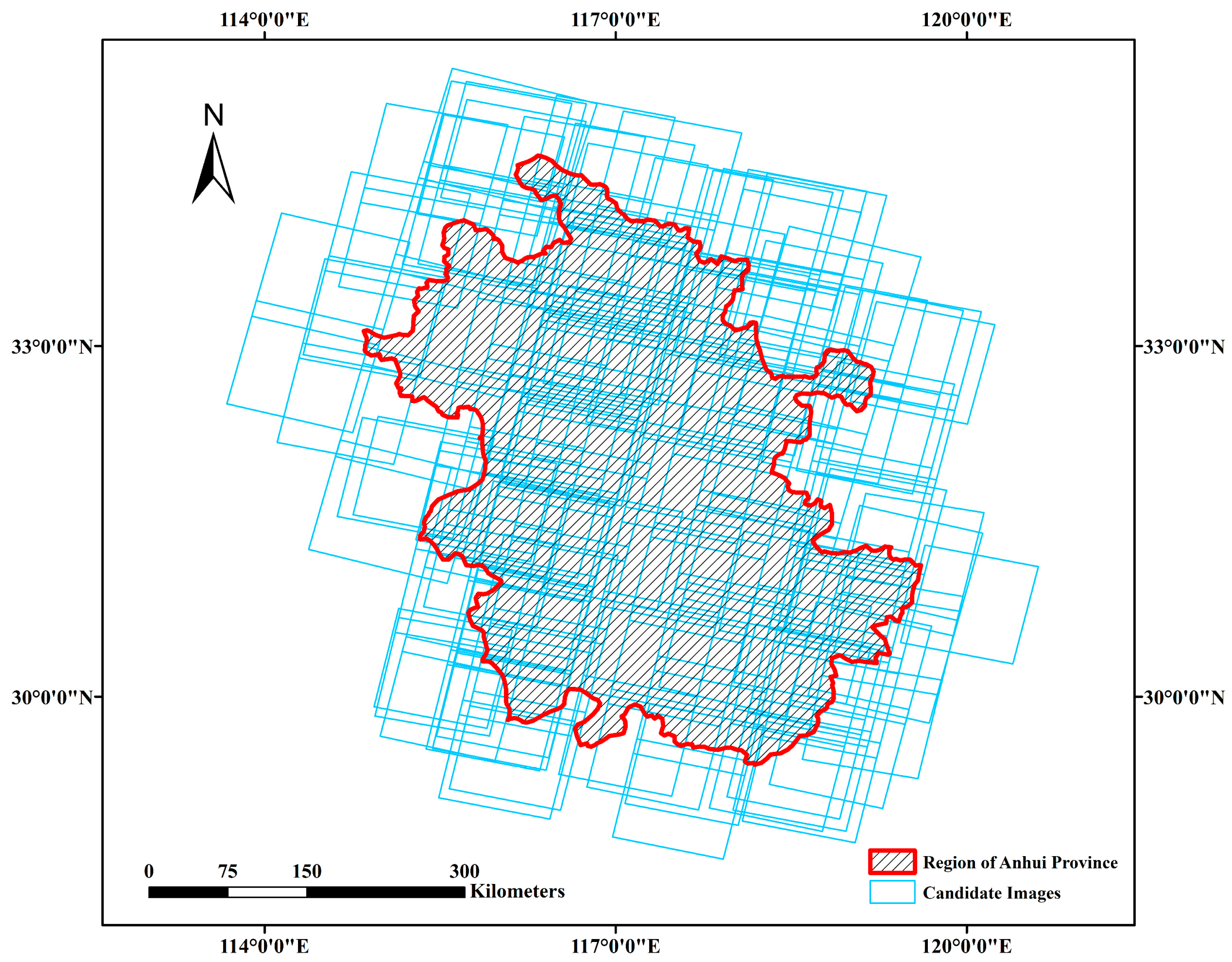
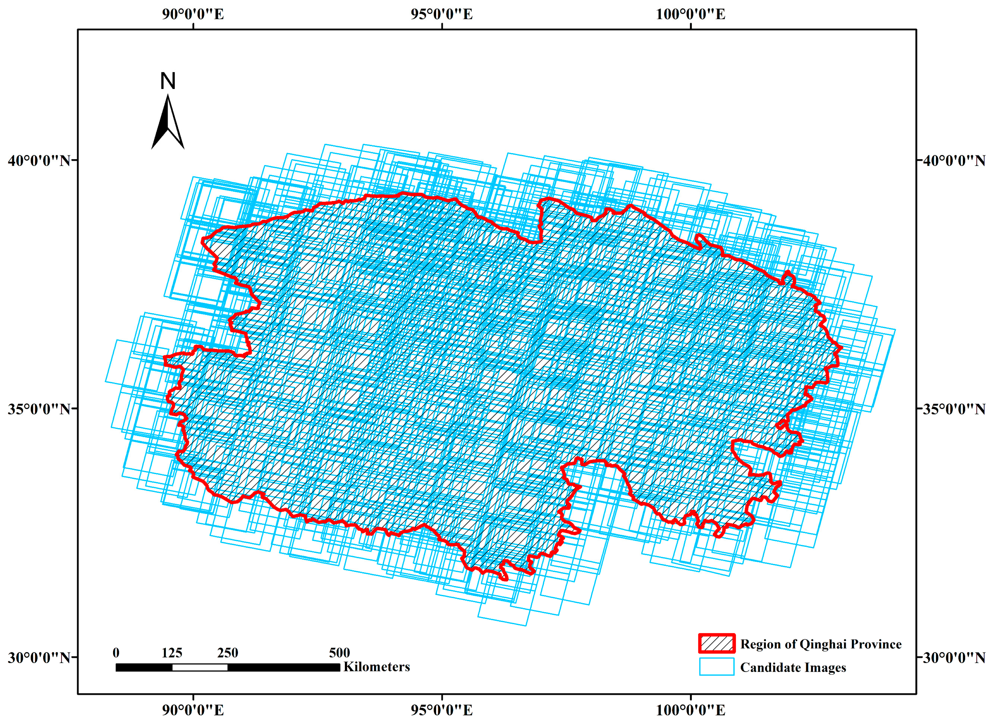
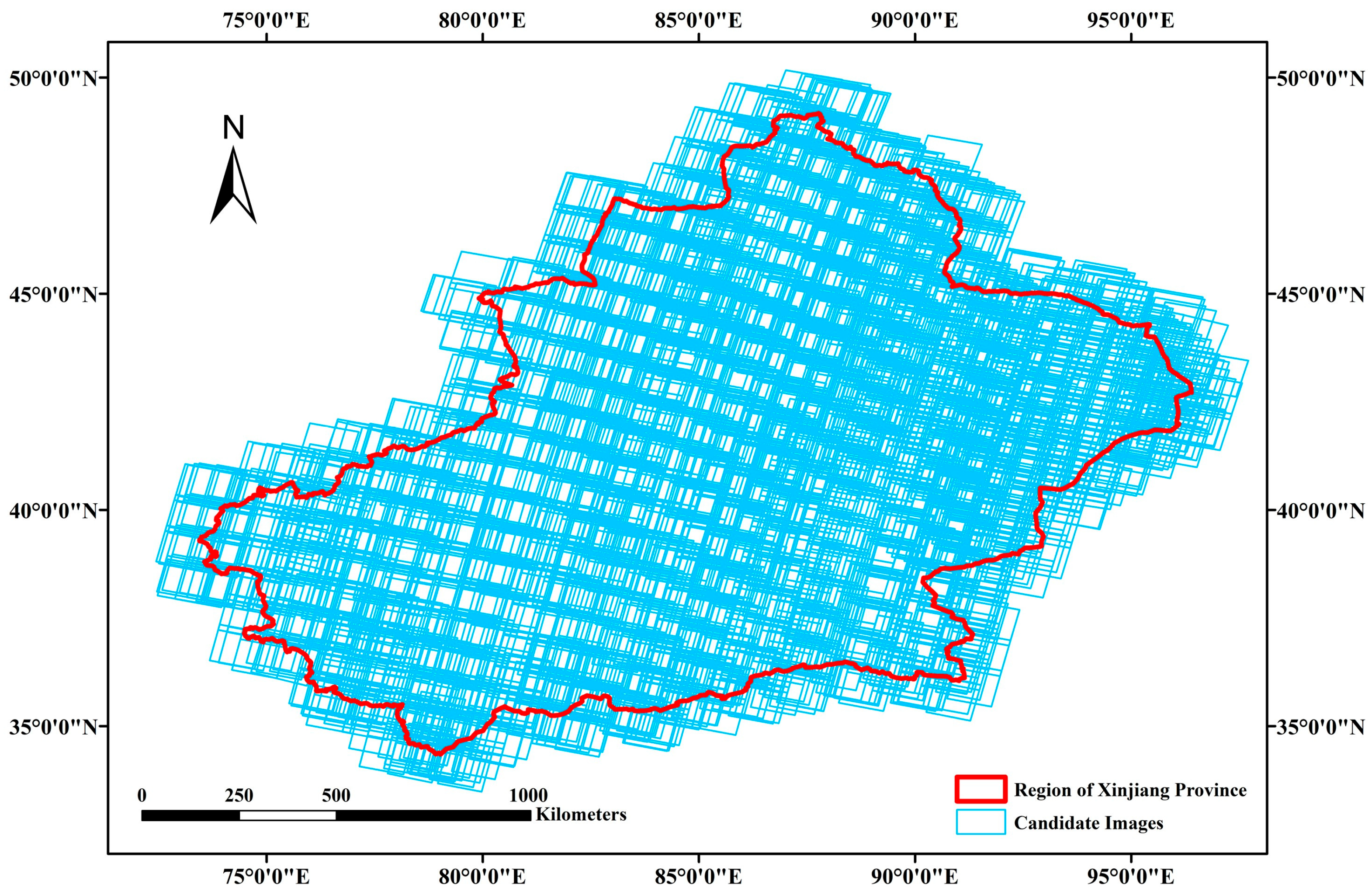
In order to more intuitively reflect the data distribution in the different geographic regions, we simulated users performing image retrieval. Specifically, the GF-6 PMS sensor data with less than 30% cloud coverage spanning from 1 January 2022 to 31 December 2022 are used in this study. By performing spatial computations, we obtained a collection of candidate images covering each experimental region. Figure 1 shows the Experimental region in this study. Figure 2, Figure 3 and Figure 4 show the data distribution in different regions.

3. Methods

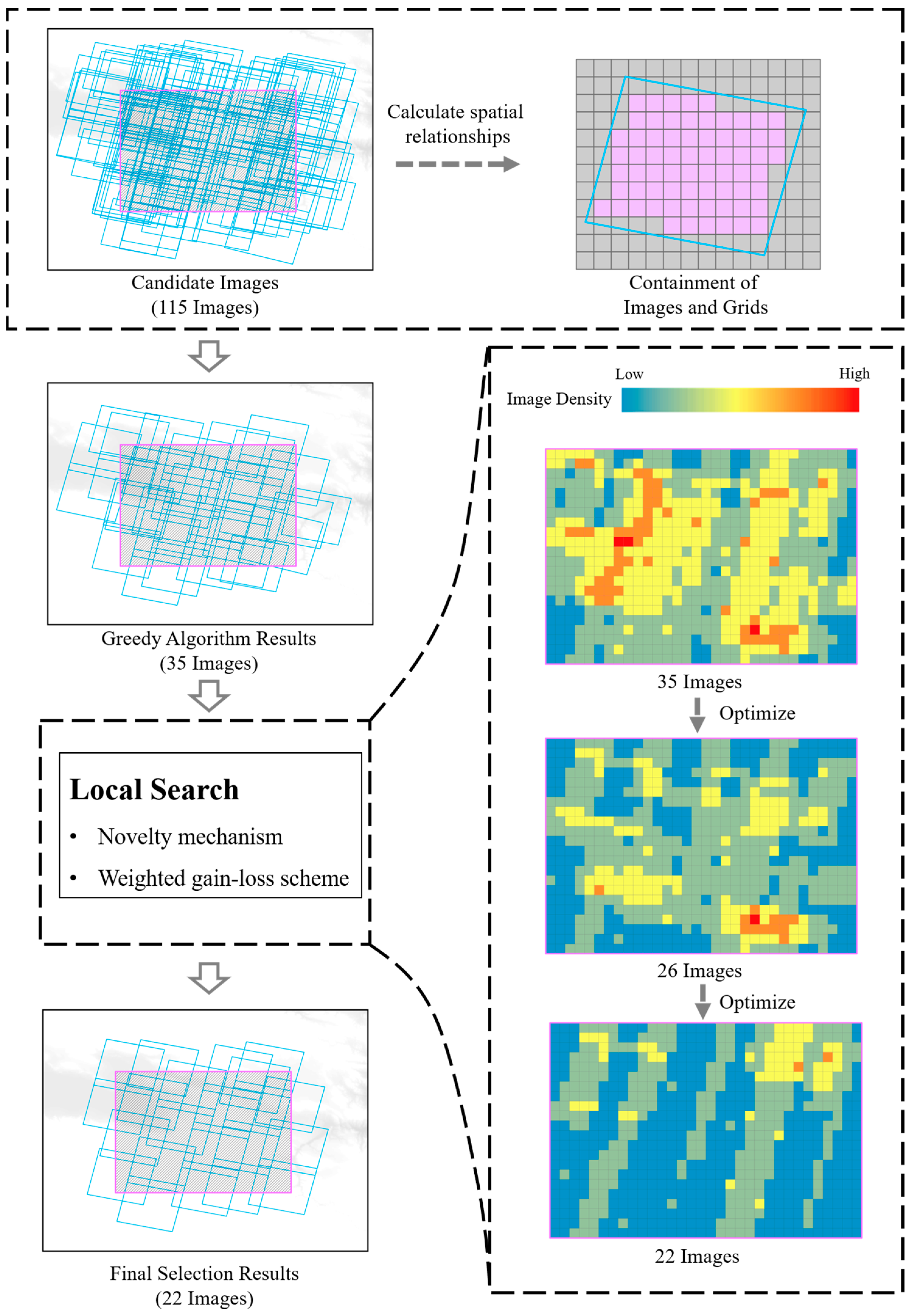
The algorithm DD-RSIRA proposed in this paper consists of the following steps: Initially, all remote sensing data intersecting with the target area are acquired as candidate datasets based on predefined screening conditions. However, these candidate datasets exhibit significant variations in attributes such as cloud cover and imaging timestamps, leading to diverse image qualities within this batch of data. To comprehensively assess image quality, factors including imaging time, cloud cover, and coverage of each image are evaluated collectively. We created global grids and obtained the grids contained in each image by spatial operations, representing the elements contained in each subset of the ensemble coverage algorithm. A greedy algorithm was performed to find the image with the optimal weight in the current situation to be added to the set by each iteration to obtain the initial solution. Finally, this paper introduces a weighted gain-loss scheme and a novel mechanism to continuously update the optimal solution through local search. The flowchart of the proposed algorithm is shown in Figure 5.

3.1. Calculating the Weight of Each Image

Based on the user’s customized filtering conditions including regional extent, satellite sensor type, imaging time, and cloud coverage, we filtered the images that satisfy the user’s needs from a huge database of remote sensing images to form a candidate dataset. In the selection process, we introduced the concept of selection cost and considered the three key indexes of cloud amount, time, and coverage. In order to balance the indexes to comprehensively evaluate the images, the coefficients of the indexes are set to 1/3 in the experiment; of course, readers can also set their own coefficients for specific scenarios. For example, the coefficients of the cloud amount can be set to very large for the pursuit of images with low cloud amounts. However, in this paper, the coefficients are balanced to pursue a comprehensive image. Specifically, C o s t c l o u d is used to evaluate the amount of cloud in the image: the less cloud occlusion, the lower the corresponding cost. C o s t t i m e is used to evaluate the time interval between the imaging time of the image and the center of the user-defined time range: the smaller the time interval, the lower the cost. C o s t c o v e r is used to evaluate the coverage of the image over the target area: the larger the coverage, the lower the corresponding cost. By considering these key indicators, we can better balance the quality and coverage of remote sensing images so as to provide users with more comprehensive and accurate data retrieval services, which also help to meet the research and application needs in different application scenarios.
Given that cloud cover, time, and coverage are quantified on distinct scales, it is imperative to perform data normalization and map the results to the 0–1 range. This normalization process allows for an equidistant rescaling of the original data. The mathematical expression is shown in Equation (1):
X n o m = X X m i n X m a x X m i n
The mathematical expression of C o s t c l o u d is shown in Equation (2):
C o s t c l o u d = c l o u d p r e s e n t c l o u d m i n c l o u d m a x c l o u d m i n
where c l o u d m a x is the highest cloud value of all the images in the candidate data set, c l o u d m i n is the lowest cloud value of all the images in the candidate data set, and c l o u d p r e s e n t is the cloud value of the image to be normalized. The smaller the cloud amount, the better the image quality and the smaller the cost.
The mathematical expression of C o s t t i m e is shown in Equation (3):
C o s t t i m e = t i m e p r e s e n t t i m e m i n t i m e m a x t i m e m i n
where, t i m e m a x is the maximum value of the time interval of all the images in the candidate dataset, t i m e m i n is the minimum value of the time interval of all the images in the candidate dataset, and t i m e p r e s e n t is the time interval of the image to be normalized. The time interval represents the difference between the image’s acquisition time and the central time of the user-defined area of interest. A smaller time interval indicates a closer alignment with the user-defined time, resulting in a lower cost.
The mathematical expression of C o s t c o v e r is shown in Equation (4):
C o s t c o v e r = c o v e r m a x c o v e r p r e s e n t c o v e r m a x c o v e r m i n
where c o v e r m a x is the maximum coverage of all images in the candidate dataset, c o v e r m i n is the minimum coverage of all images in the candidate dataset, and c o v e r p r e s e n t is the coverage of the image to be normalized. The larger the coverage, the more parcels are covered by the image and the smaller the cost.
According to different remote sensing application scenarios, the weight coefficients of cloud amount, time interval, and coverage are set as w c l o u d , w t i m e , and w c o v e r . The comprehensive cost C of the remote sensing images is given by Equation (5). In this paper, the coefficients of the metrics are set to 1/3 in order to evaluate the images in a comprehensive way.
C = w c l o u d C o s t c l o u d + w t i m e C o s t t i m e + w c o v e r C o s t c o v e r
w c l o u d + w t i m e + w c o v e r = 1 ,  
0   C o s t c l o u d 1 ,     0 C o s t t i m e 1 ,     0 C o s t c o v e r 1

3.2. Calculate the Inclusion Relationship between the Image and the Grid

Establishing the global grids is a crucial step in our methodology. Utilizing spatial computations, we derive the spatial relationships between each image and the grid cells. In this context, each image is conceptualized as a subset, and the grid cells it encompasses are considered as the elements within that subset. This strategic transformation effectively reformulates the regional optimal coverage problem into a set covering problem. This conversion streamlines the optimization process, rendering it more amenable to the application of set-covering algorithms, ultimately facilitating the efficient discovery of an optimal solution.

3.3. Optimal Regional Coverage of Remote Sensing Image

3.3.1. Compute the Compulsory Subsets

A subset e i   is a unit element if only one subset contains the element. Moreover, a subset S i is a forced subset compulsory subset if the subset S i includes at least one unit element. Because all elements should be covered, including the unit elements, the forced subsets must be present in the final result by setting the set of forced subsets to R c .
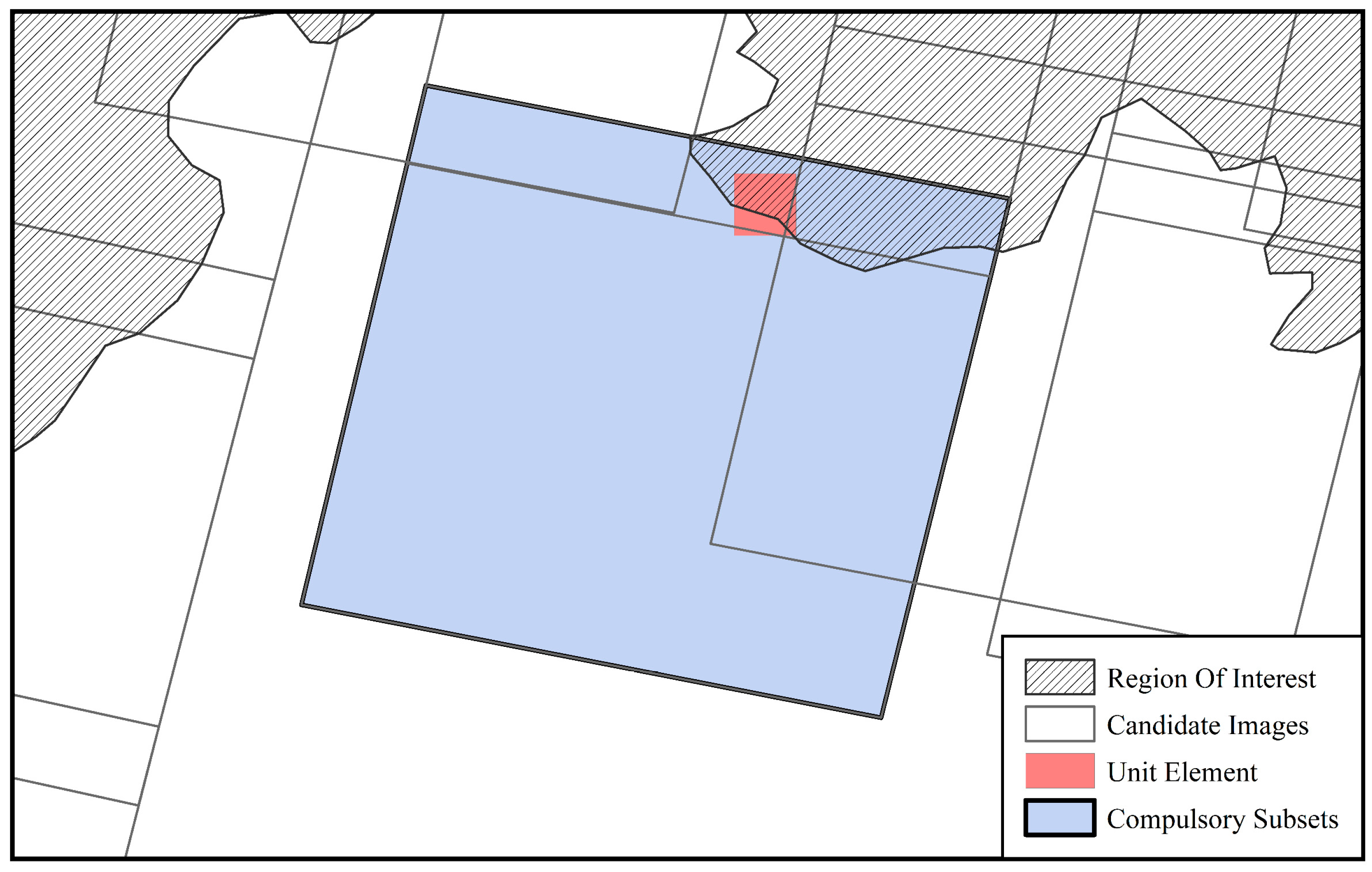
As shown in the figure below, the shaded region is the region of interest, and the red grid is one of the global grids. Take the red grid in the figure as an example: it intersects with the region of interest so it needs to be included in the consideration, but this red grid is completely covered by only one image, and the rest of any candidate images fail to cover this grid. Therefore, the red grid is a unit element, and this image is a forced subset, and it will be forced to be selected as shown in Figure 6.

3.3.2. Greedy Computation

The step involves treating the grids covered by the candidate set as elements to be covered. A subset with the minimal cost is systematically chosen from the candidate set to cover all these elements. In each iteration, the cost associated with each image under the current conditions is computed. This entails calculating the cost incurred for each image chosen for inclusion in the collection, as well as determining the elements already covered by the current result set. Subsequently, in each iteration, the selection of the subset involves considering the combined cost of covering the remaining uncovered elements within the current state, including both the number of uncovered elements and the image quality. The selection cost is calculated based on C a d d (in Section 3.3.3). This cumulative process continues until all elements are satisfactorily covered, ultimately yielding a locally optimal solution through the greedy algorithm.

3.3.3. Local Search

After the greedy algorithm, an initial solution R is obtained, and this phase performs a local search of R. At each iteration, the solution R is optimized by modifying R, i.e., by performing additions and deletions of subsets while ensuring the completeness of the result in terms of coverage of all the elements. Whenever a less costly set of results is found, an update is performed using R’ to record the current best solution. In this paper, we introduce a weighted gain-loss scheme and a novel mechanism for local search of the optimal solution.
  • Weighted gain-loss scheme
This paper employs the concept of subset element gain, denoted as G i , to represent the number of uncovered elements that would be covered upon incorporating subset S i into the result set R. The inclusion of subsets with larger G i values results in the coverage of a greater number of elements within the result set. Therefore, subsets with greater element gain should be added to the result set with lower associated costs. C a d d represents the cost of image addition (Equation (8)). In this paper, the coefficients of the metrics are set to 1/3 in order to evaluate the images in a comprehensive way.
C o s t G = G m a x G i G m a x G m i n
C a d d = w c l o u d C o s t c l o u d + w t i m e C o s t t i m e + w G C o s t G
w c l o u d + w t i m e + w G = 1 ,
0   C o s t c l o u d 1 ,     0 C o s t t i m e 1 ,     0 C o s t G 1
When selecting images to add to the result set, both the subset element gain and image quality need to be considered to calculate their combined cost. The image with the lowest cost is continually selected to be added to the result set R until R covers all elements.
In the above, a subset element gain G i is introduced to represent the number of uncovered elements covered by the addition of the image S i to R. In addition, a new metric subset element loss L i is introduced to indicate the number of elements whose original coverage becomes uncovered after S i is removed from R. At the beginning of each iteration, the current result R is first checked to see if it satisfies the inclusion of all elements. If satisfied, all redundant subsets in R are then searched and deleted; for example, if all elements contained in the subset S i are contained by other subsets in R, i.e., L i is 0, then S i is a redundant subset, and the deletion of the redundant subset has no effect on the completeness of the result. The current optimal solution R’ is updated after deletion. Next, a subset is removed from R. The removed subset includes the image whose removal cost C r m is minimized, i.e., the removal of this image minimizes the loss to the entire result set. The formula for calculating C r m is shown in Equation (13). In this paper, the coefficients of the metrics are set to 1/3 in order to evaluate the images in a comprehensive way.
C o s t L = L i L m i n L m a x L m i n
C r m = w c l o u d C o s t c l o u d + w t i m e C o s t t i m e + w L C o s t L
w c l o u d + w t i m e + w L = 1 ,
0   C o s t c l o u d 1 ,     0 C o s t t i m e 1 ,     0 C o s t L 1
In each process of removing a subset, the subset element loss L i of the images in the current set is calculated, and the removal cost C r m of each image is calculated, which indicates the size of the loss of removing the image to the whole result set, and the image with the smallest C r m is removed from the set.
b.
Novel mechanism
The C a d d metrics can be effectively evaluated to add the image with the lowest cost to R; however, it has been shown that if only a greedy strategy is used, it will lead to the search stopping and the inability to find a better solution. In order to solve the problem of search stagnation, this paper adopts a novel mechanism. In each iteration, based on the C a d d metric, the algorithm has a probability of p to select the suboptimal image to be added to R. Otherwise, the optimal image will be selected. In this experiment, the p-value was set to 0.3.
The optimization of the result set is accomplished through an intensive iterative process. The termination condition is that the optimal total cost within 50 iterations remains constant. The detailed steps of optimal regional coverage of remote sensing images are presented in Algorithm 1. The input I of the algorithm is a candidate set of remote sensing images queried according to user-defined conditions, and the grid range covered by the candidate set is the target range covered by the final result. According to the algorithm, the optimal area coverage result is finally output.
Algorithm 1. Optimal regional coverage of remote sensing image
Input I: Candidate data of remote sensing image
Output R*: Optimal region coverage result
1: Calculate the unit elements e and compulsory subsets R c .
2: Remove the unit elements e from the elements E to be covered to get E*.
3: Calculate the initial solution R by greedy algorithm.
4: R* R
5: While the abort criterion is not met:
6:   if R covers E*
7:     if cost(R) < cost(R*)
8:       R* R.
9:     Compute C r m for each subset in the current state.
10:      Remove a small subsets which includes the subset with the smallest C r m .
11:    Compute C a d d for each subset in the current state.
12:    With probability p select the suboptimal C a d d , otherwise, select the optimal one.
13:    Add the corresponding subset to R*.
14:  R* R*   R c
15:  Output the final result R*

3.4. Data Distribution Assessment Indicators

In our research, to facilitate an objective and quantitative assessment of the distribution of outcomes, we have introduced several evaluation metrics. The introduction of these metrics is aimed at providing a more comprehensive approach to analyzing the results and establishing quantitative indicators:
  • Coverage Ratio (CR): This metric represents the total coverage of the resulting image result set as a proportion of the region of interest.
  • Image Density (ID): The number of images of each grid is calculated as the image density for that grid.
  • Average Image Density (AID): The average of the image densities of all grids is calculated to represent the overall density of the result.
  • Redundancy Ratio (RR): This metric indicates the amount of redundancy in the coverage area of the resulting image result set. The formula is as follows:
    R R = i I S i S A 1
    where S i is the area of the ith selected image and S_A is the area of the entire region of interest. RR values are expressed in percentages.
  • Utilization Ratio (UR): This metric represents the average utilization rate of images. The formula is as follows:
    U R = ( 1 i I S i S o t h e r S i ) / n
    where S i is the area of the ith selected image, S o t h e r is the area of the image concatenation excluding the ith image, and n is the number of images. UR values are expressed as a percentage.

4. Results

In this study, we chose the method proposed by Li et al. [23] as well as the greedy algorithm as references in order to provide an in-depth evaluation of our research methodology. We applied these different remote sensing image retrieval methods on different datasets from several geographical regions in order to compare and analyze their performance comprehensively. The effectiveness of this experimental methodology is validated through the performance of the different algorithms.

4.1. Analysis of the Distribution of Results

4.1.1. Quantitative Evaluation

In order to quantitatively analyze the results of the proposed method and the other two methods, this paper uses the number of result sets, CR, AID, RR, and UR indicators for the statistics and evaluation of the distribution of results. The results of each indicator are summarized in the Table 2.
From Table 2, it is evident that all three methods prioritize ensuring the coverage of remote sensing image sets while reducing the data to varying degrees. The method presented in this paper significantly outperforms the other two methods across all indicators, showing a pronounced optimization effect in terms of the number of result sets, AID, RR, and UR metrics.
In comparison to the original data, all three methods exhibit improvements. However, Li et al.’s method produces a larger number of result sets. This is primarily attributed to their approach, which is based on grid-based selection. This method involves traversing each grid; calculating the comprehensive cost of covering all remote sensing images within each grid; considering factors such as cloud cover, time, and coverage range; and selecting the images with optimal weights to form the final dataset. This approach does not effectively address the image coverage issue, resulting in a higher number of result sets.
On the other hand, the greedy algorithm is based on a greedy strategy that employs the concept of set cover. At each step, it selects the best solution given the current state without considering the global optimal solution. This implies that the greedy algorithm tends to quickly find a local optimum. In contrast, the method proposed in this paper is a local search based on the greedy algorithm, utilizing a weighted gain-loss scheme and novel mechanism. It continually approximates the optimal solution. Ultimately, the results of this method outperform both of the aforementioned methods, effectively reducing redundant data. In comparison to Li et al.’s method, in the Anhui region, the redundancy ratio decreased from 359% to 214%; in the Qinghai region, it decreased from 302% to 205%; and in the Xinjiang region, it decreased from 263% to 172%. The number of images was optimized by 20%. In comparison to the greedy algorithm, the redundancy rates in each region were reduced by over 20%. Moreover, the results obtained using the method described in this paper indicate higher UR, with an improvement of 4% to 8%. It is clear from the AID metrics that the proposed algorithm performs excellently for computation at different image densities and is able to further reduce the image density. This method further enhances data distribution, resulting in reduced redundancy and increased image utilization in the retrieval results.

4.1.2. Visualization and Analysis

To further validate the effectiveness of the methodologies proposed in this paper in terms of data distribution, we conducted a visual representation of the raw data and the results obtained from the three different approaches. This visualization entailed an assessment of the image count covering each grid, thereby functioning as a density evaluation for individual grid cells. We used a color gradient from blue to red to visually and graphically show the data density in each region under the influence of the different methods.
  • Anhui dataset
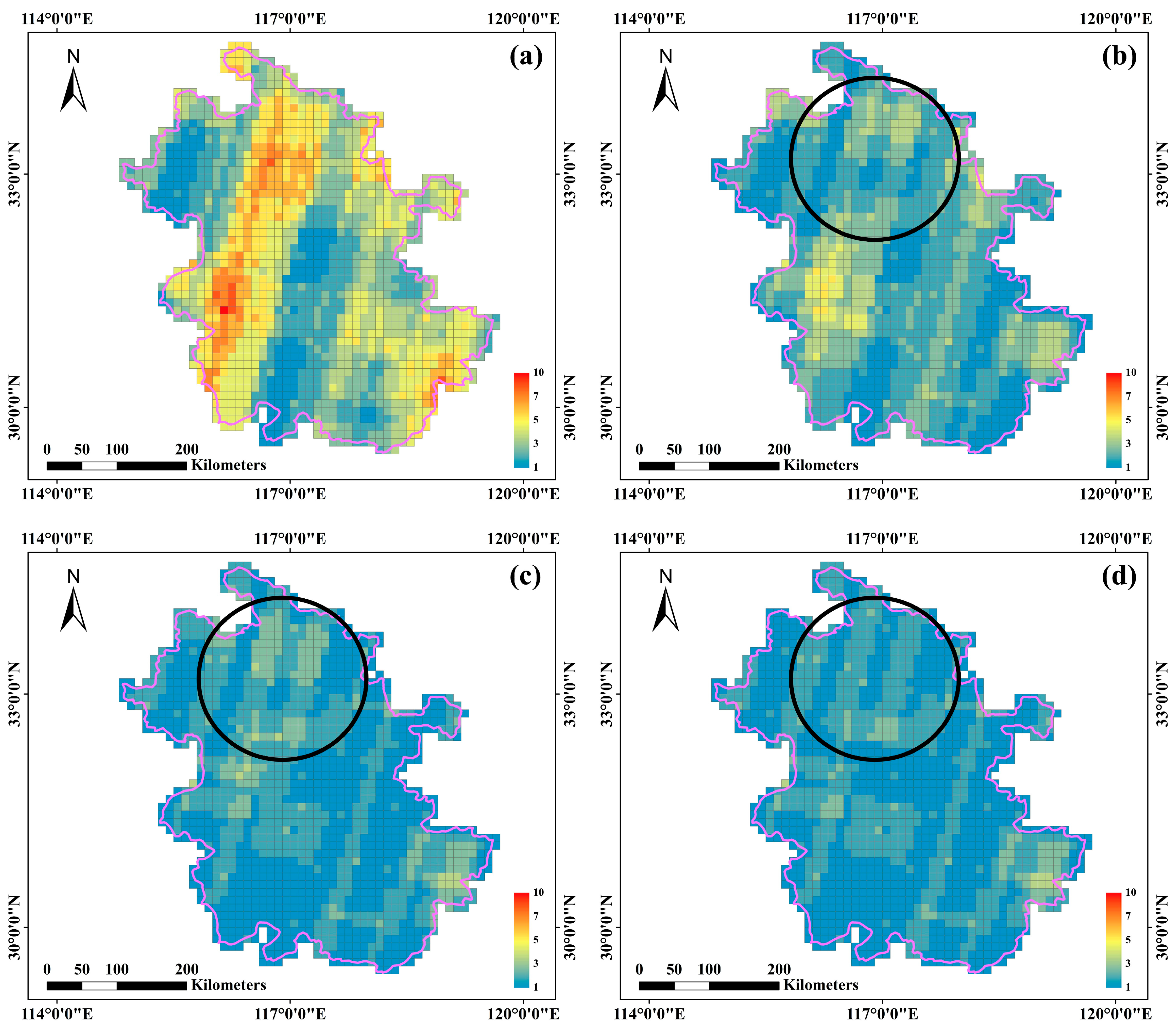
As shown in Figure 7, the redundancy part is in the form of obvious bars in the candidate dataset of Anhui Province. It can be seen that the dense part of the data is significantly improved after processing using the method of Li et al. Although the method greatly reduces the amount of redundancy, it is still clearly visible that there are striped yellow dense regions, and the effect of de-redundancy is limited. The result of the greedy algorithm is better than the method of Li et al., showing less redundancy in the striped dense region. The method in this paper performs better than the greedy algorithm in some localized regions (e.g., black circles).
2.
Qinghai dataset
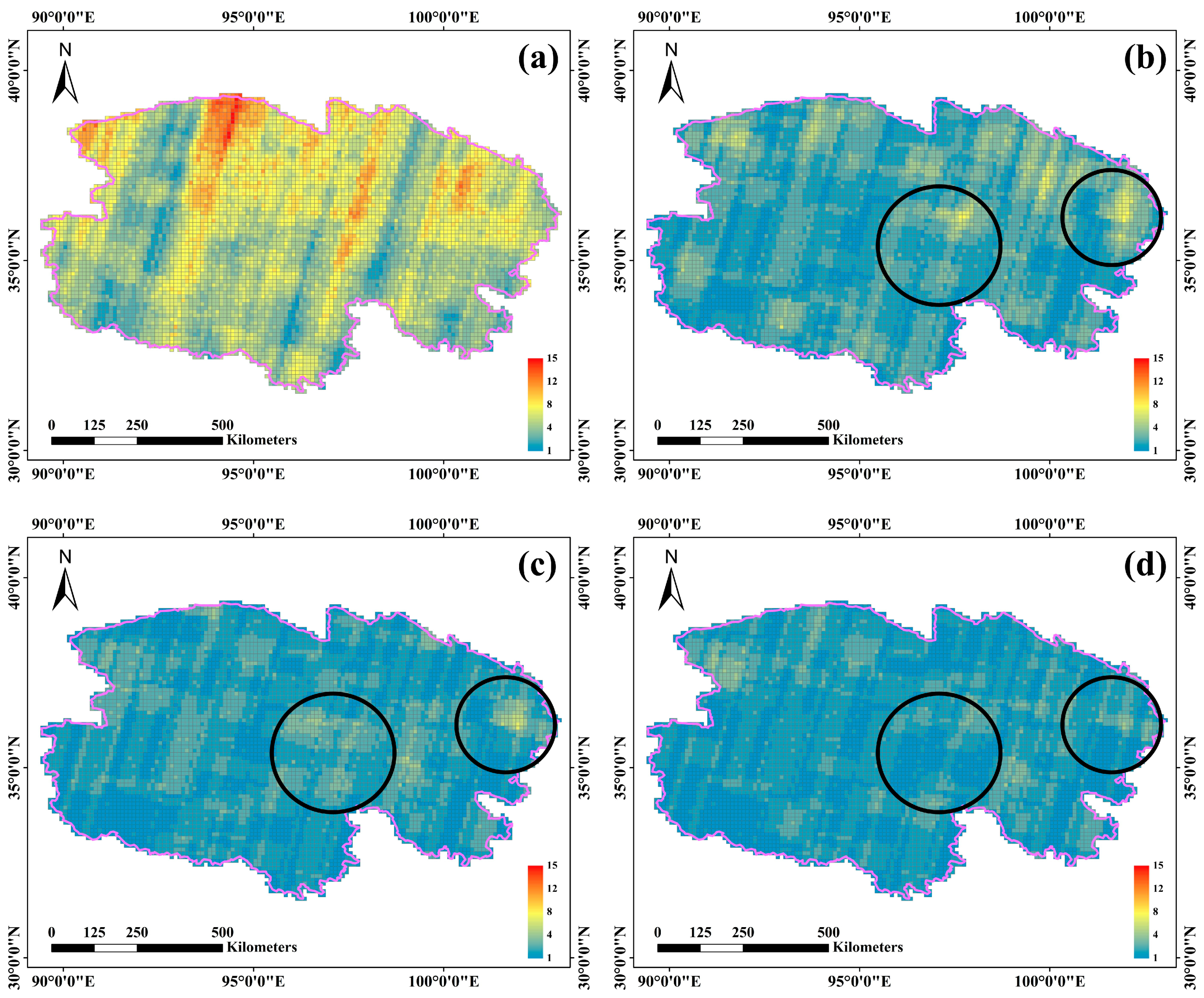
The density distribution of the result set in the Qinghai Province is shown in Figure 8. The density map of the candidate dataset shows that the data density is larger in the northern part of the Qinghai Province. After processing using Li et al.’s method, the data density in the north and east is still larger, with obvious bright yellow areas. After processing using the greedy algorithm, the region in the east still has a darker yellow color. In contrast, our method optimizes the processing of the data-dense areas in the north and east, avoiding obvious yellow areas and having an overall bluish hue. This method produces a more even distribution of data density and therefore the best overall performance.
3.
Xinjiang dataset
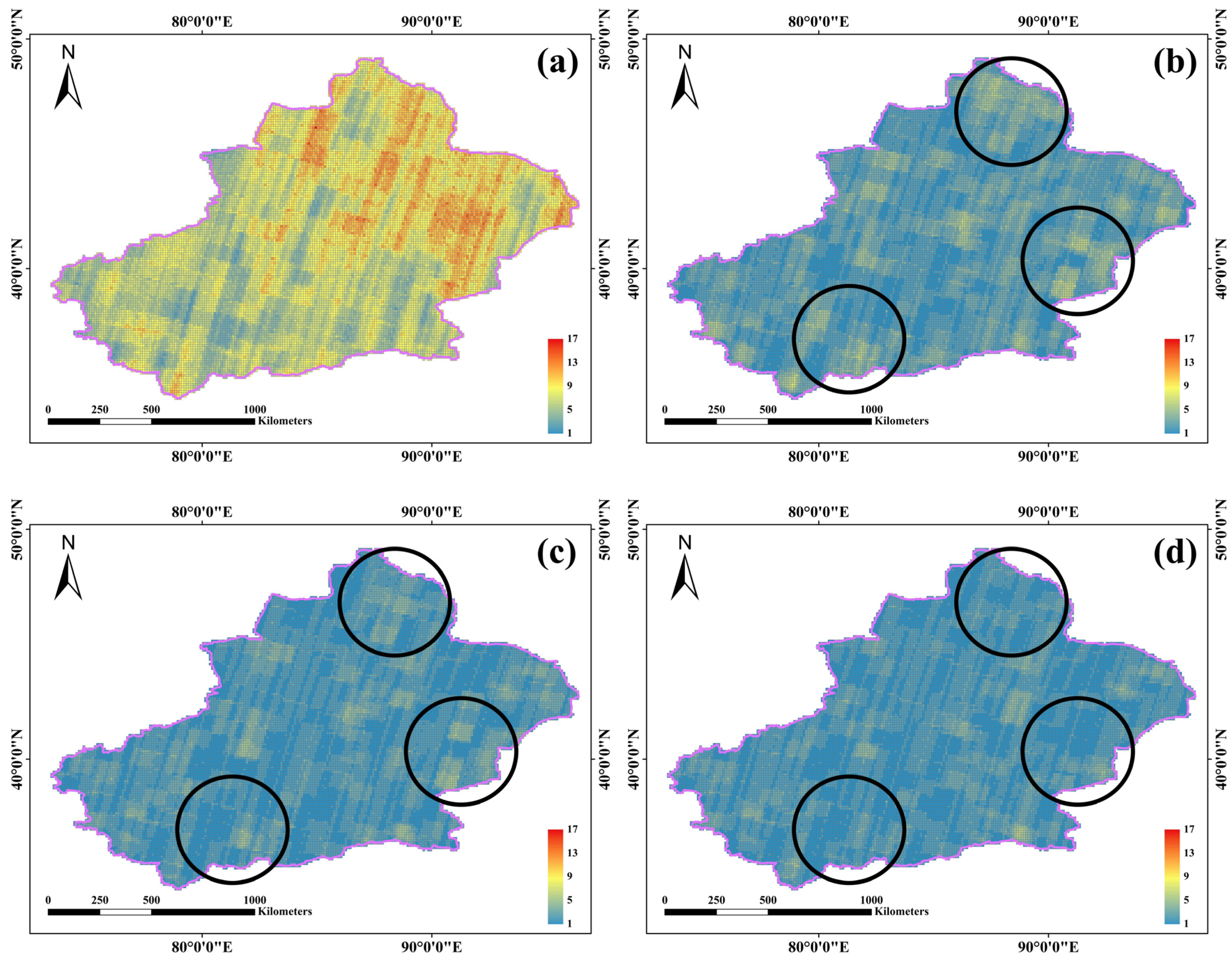
Figure 9 shows that there is a large amount of redundant data in the candidate dataset for the Xinjiang region, with a considerable amount of the region appearing in yellow and red colors. Although Li et al.’s method effectively reduces the data redundancy in this region, the visual representation still shows distinct yellow patches, and there is still a clear case of data density. The result of the greedy algorithm is slightly better than Li et al.’s method, but the density is still higher in some regions (e.g., black circles). Our method is better optimized on all these regions. The overall color is smoother, indicating that the overall data density has been reduced.

4.2. Quality Evaluation of Images

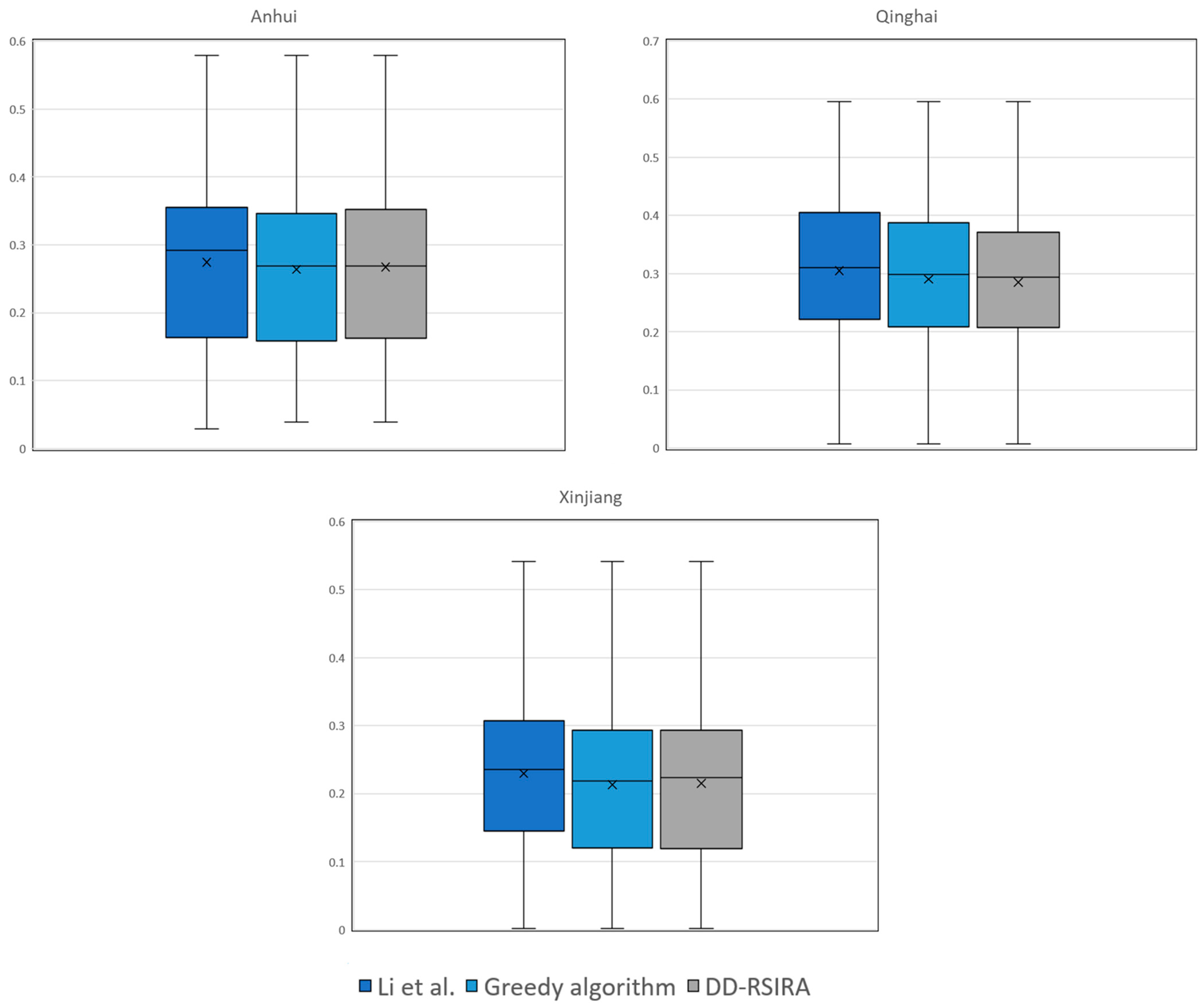
In this paper, in order to verify the quality of the image result set of the proposed algorithm, the combined cases of cloud amount and time are used as the image screening cost, and the weighting factors of cloud amount and time are set to ½, respectively. The lower the cost of the image is, the better the quality of the image. Under the same input conditions, the image cost distributions of the results of Li et al.’s method, the greedy algorithm, and the DD-RSIRA algorithm are counted, respectively. The box plot is used to show their distributions (Figure 10). The metrics of the box plot are shown in Table 3: Min represents the minimum value of the image cost in the data; Q1 represents the lower quartile of the image cost, i.e., the value at 25%; Q2 represents the median of the image cost; Q3 represents the upper quartile of the image cost, i.e., the value at 75%; and Max represents the maximum value of the image cost.
The box plot shows the distribution of image cost under the different methods. In the box plot, the center line is the median image cost, which indicates the median level of the resultant dataset: the smaller the cost, the better the image quality. The upper quartile and lower quartile of the box account for 50% of the data in the box, so the main box reflects the distribution of data quality to some extent. From the above experimental data, it can be seen that the Max values of the three methods are the same, i.e., the maximum values of the image cost are the same for all of them, which indicates that the method proposed in this paper will not select images with too-poor quality in the retrieval process in order to pursue the coverage. Because cloud amount, time, and coverage are considered together in this paper, the method of Li et al. is not further optimized for cloud amount and time considerations. This method has a high image cost due to the weighting of the coverage. The experimental results in the Anhui Province show that the image cost of DD-RSIRA is slightly higher than that of the greedy algorithm. The data quality in Qinghai Province is the best among the three methods, while the indicators in Xinjiang are in an up-and-down state. From the experimental results, it can be seen that, although the data quality of each method is not consistent, the deviation of the DD-RSIRA method proposed in this paper from the greedy algorithm is only 2%, which fully guarantees the image quality.

5. Discussion

In this investigation, we employed Li et al.’s method and the greedy algorithm as benchmarks to rigorously evaluate and validate our proposed remote sensing image preference methodology, termed DD-RSIRA. Through the application of these diverse remote sensing image retrieval approaches across various datasets spanning different geographical regions, we conducted a comprehensive comparative analysis to assess their performance. The outcomes of these thorough comparisons and analyses serve to affirm the efficacy of our research methodology. Based on the results, all three methods are able to reduce data in a way that ensures CR. However, our DD-RSIRA method shows significant advantages in all evaluation metrics. In particular, DD-RSIRA shows significant performance improvements in the number of result sets, AID, RR, and UR.
All three methods achieved some improvements as compared to the original data. However, Li et al.’s method generates the largest number of result sets, which is mainly due to the fact that their method is based on grid filtering, which leads to difficulties in dealing with the image coverage problem efficiently, and thus the amount of redundant data in the result set is relatively large. The greedy algorithm, on the other hand, iterates quickly to find the local optimal solution, resulting in the result set still having redundancy in some regions. In contrast, our proposed DD-RSIRA method introduces a weighted gain-loss scheme and a novel mechanism that significantly optimizes the result distribution via local search. This optimization successfully diminishes data redundancy while enhancing the overall image utilization. To further validate the improvement of the result distribution by our proposed method, we visualized the result set. The distribution of each region was demonstrated by counting the number of times each grid was covered and color-rendering the results. By comparing the three experimental regions of Anhui, Qinghai, and Xinjiang, it can be seen that although Li et al.’s algorithm adeptly handles dense data by reducing redundancy, its reliance on grid-based filtering causes limitations. The greedy algorithm, while effective, still exhibits dense data concentrations in specific regions. DD-RSIRA, optimized from the groundwork of the greedy algorithm, elevates the treatment of local regions, resulting in a more uniform and reduced overall density.
Furthermore, we evaluated the quality of the results using box plots. Although the DD-RSIRA method significantly reduces data redundancy, the method does not sacrifice data quality in the pursuit of greater coverage. Across various experiments conducted in the different regions, we observed a slight decrease in data quality for the DD-RSIRA method in the Anhui Province. However, its performance notably excelled in the experiments conducted in the Qinghai and Xinjiang regions. This variation in performance might be attributed to the relatively lower data density in the Anhui Province, which results in fewer image options during the local search process. In contrast, the higher data density in Qinghai and Xinjiang provided more opportunities to select superior-quality images for ensemble replacement, consequently enhancing the performance of DD-RSIRA in these areas. Hence, DD-RSIRA exhibits superior performance in regions characterized by higher data density. Moreover, although fluctuations in image quality were observed during the local search, these fluctuations remained minimal at approximately 2%. This marginal variance minimally impacts the overall image quality, ensuring a certain level of data quality preservation.
In summary, the optimal area coverage problem of satellite images is effectively improved by the method presented in this paper. In addition, the current problems for seabed geological investigation as well as underwater archaeology have generated underwater imaging technology [41,42]. The retrieval of underwater remote sensing images may not be fully adapted to this method, because the method in this paper is for surface coverage. However, underwater remote sensing images can also draw on the surface processing, using the corresponding indicators to construct the selection cost and realize the optimal coverage problem of underwater remote sensing images by means of set coverage.

6. Conclusions

This paper introduces a high-density data remote sensing image retrieval algorithm (DD-RSIRA) which aims to solve the remote sensing image retrieval challenges in areas with dense data. DD-RSIRA is committed to providing high-quality solutions by ensuring no loss of coverage while taking into account data overlap and data quality. To achieve this goal, the algorithm employs an enhanced search for the optimal solution through a local search approach and introduces a weighted gain-loss scheme and a novel mechanism strategy. In our comparative study, we benchmarked the DD-RSIRA against the greedy algorithm and the method proposed by Li et al. The experiments decisively illustrated the superior performance of DD-RSIRA. It outperforms other algorithms in terms of the number of results, density, and redundancy. Compared to the greedy algorithm, it reduces redundancy by about 30% and improves the average image utilization by 4% to 8%. Moreover, DD-RSIRA contributes to maintaining the quality of remote sensing images, establishing a robust foundation for remote sensing data acquisition and analysis. DD-RSIRA is expected to improve the effectiveness and efficiency of these applications by optimizing the retrieval of remote sensing images in dense data, which are used in a variety of practical areas such as GIS, resource management, and environmental monitoring.

Author Contributions

X.L. designed the experiments and wrote the manuscript; W.L. supervised the study and reviewed the draft paper; S.L. revised the manuscript and gave some appropriate suggestions. All authors have read and agreed to the published version of the manuscript.

Funding

This research received no external funding.

Data Availability Statement

The data presented in this study are available on request from the corresponding author. The data are not publicly available due to institutional confidentiality.

Acknowledgments

We thank the China Remote Sensing Satellite Ground Station for providing remote sensing metadata and for supporting this experiment.

Conflicts of Interest

The authors declare no conflicts of interest.

References

  1. Shi, S.; Zhong, Y.; Zhao, J.; Lv, P.; Liu, Y.; Zhang, L. Land-Use/Land-Cover Change Detection Based on Class-Prior Object-Oriented Conditional Random Field Framework for High Spatial Resolution Remote Sensing Imagery. IEEE Trans. Geosci. Remote Sens. 2022, 60, 1–16. [Google Scholar] [CrossRef]
  2. Nemni, E.; Bullock, J.; Belabbes, S.; Bromley, L. Fully Convolutional Neural Network for Rapid Flood Segmentation in Synthetic Aperture Radar Imagery. Remote Sens. 2020, 12, 2532. [Google Scholar] [CrossRef]
  3. Zhu, X.; Guo, R.; Liu, T.; Xu, K. Crop Yield Prediction Based on Agrometeorological Indexes and Remote Sensing Data. Remote Sens. 2021, 13, 2016. [Google Scholar] [CrossRef]
  4. Du, P.; Liu, S.; Xia, J.; Zhao, Y. Information fusion techniques for change detection from multi-temporal remote sensing images. Inf. Fusion 2013, 14, 19–27. [Google Scholar] [CrossRef]
  5. Tong, X.-Y.; Xia, G.-S.; Lu, Q.; Shen, H.; Li, S.; You, S.; Zhang, L. Land-cover classification with high-resolution remote sensing images using transferable deep models. Remote Sens. Environ. 2020, 237, 111322. [Google Scholar] [CrossRef]
  6. Yu, Q.; Shang, Y.; Liu, X.; Lei, Z.; Li, X.; Zhu, X.; Liu, X.; Yang, X.; Su, A.; Zhang, X.; et al. Full-parameter vision navigation based on scene matching for aircrafts. Sci. China Inf. Sci. 2014, 57, 1–10. [Google Scholar] [CrossRef]
  7. Ivancsits, C.; Ricky Lee, M.F. Visual navigation system for small unmanned aerial vehicles. Sens. Rev. 2013, 33, 267–291. [Google Scholar] [CrossRef]
  8. Durbha, S.S.; King, R.L.; Shah, V.P.; Younan, N.H. Image information mining for coastal disaster management. In Proceedings of the 2007 IEEE International Geoscience and Remote Sensing Symposium, Barcelona, Spain, 23–28 July 2007; pp. 342–345. [Google Scholar]
  9. Panteras, G.; Cervone, G. Enhancing the temporal resolution of satellite-based flood extent generation using crowdsourced data for disaster monitoring. Int. J. Remote Sens. 2018, 39, 1459–1474. [Google Scholar] [CrossRef]
  10. Dell’Acqua, F.; Gamba, P. Query-by-shape in meteorological image archives using the point diffusion technique. IEEE Trans. Geosci. Remote Sens. 2001, 39, 1834–1843. [Google Scholar] [CrossRef]
  11. Rivest, S.; Bédard, Y.; Proulx, M.-J.; Nadeau, M.; Hubert, F.; Pastor, J. SOLAP technology: Merging business intelligence with geospatial technology for interactive spatio-temporal exploration and analysis of data. ISPRS J. Photogramm. Remote Sens. 2005, 60, 17–33. [Google Scholar] [CrossRef]
  12. Reichman, O.J.; Jones, M.B.; Schildhauer, M.P. Challenges and Opportunities of Open Data in Ecology. Science 2011, 331, 703–705. [Google Scholar] [CrossRef] [PubMed]
  13. Wulder, M.A.; Loveland, T.R.; Roy, D.P.; Crawford, C.J.; Masek, J.G.; Woodcock, C.E.; Allen, R.G.; Anderson, M.C.; Belward, A.S.; Cohen, W.B.; et al. Current status of Landsat program, science, and applications. Remote Sens. Environ. 2019, 225, 127–147. [Google Scholar] [CrossRef]
  14. Carrasco, L.; O’Neil, A.W.; Morton, R.D.; Rowland, C.S. Evaluating Combinations of Temporally Aggregated Sentinel-1, Sentinel-2 and Landsat 8 for Land Cover Mapping with Google Earth Engine. Remote Sens. 2019, 11, 288. [Google Scholar] [CrossRef]
  15. Gorelick, N.; Hancher, M.; Dixon, M.; Ilyushchenko, S.; Thau, D.; Moore, R. Google Earth Engine: Planetary-scale geospatial analysis for everyone. Remote Sens. Environ. 2017, 202, 18–27. [Google Scholar] [CrossRef]
  16. Baumann, P.; Mazzetti, P.; Ungar, J.; Barbera, R.; Barboni, D.; Beccati, A.; Bigagli, L.; Boldrini, E.; Bruno, R.; Calanducci, A.; et al. Big Data Analytics for Earth Sciences: The EarthServer approach. Int. J. Digit. Earth 2016, 9, 3–29. [Google Scholar] [CrossRef]
  17. Zuo, X.; Xiong, M.; Huang, Z.; Zang, W.; Shang, D. A Full Coverage Retrieval Mode and Method for Remote Sensing Tile Data. J. Henan Univ. Nat. Sci 2018, 48, 299–308. [Google Scholar]
  18. Ni, R. A JSON-based heterogeneous data query method. Radio Commun. Technol. 2013, 39, 73–76. [Google Scholar]
  19. Wang, S. Research on capacity demand estimation method of remote sensing data service system. Radio Eng. 2013, 43, 61–64. [Google Scholar]
  20. Pan, J.; Chen, L.; Wang, M. A Full-Coverage Remote Sensing Image Screening Method Based on Quality Grading and Spatio-Temporal Constraints. CN114842184A, 2 August 2022. [Google Scholar]
  21. Huang, Z.; Wang, D.; Yu, T.; Zhang, S.; He, F. A Single-Time-Phase Full-Coverage Remote Sensing Data Retrieval Method Based on Grid Compensation. CN107291801A, 24 October 2017. [Google Scholar]
  22. Sun, K.; Chen, J.; Wang, M.; Li, F.; Wang, S.; Shuai, T. A Fast Retrieval Method for Remote Sensing Images Based on Circular Region Description. CN111984808A, 24 November 2020. [Google Scholar]
  23. Li, F.; You, S.; Wei, H.; Wei, R.; Chen, L. Filtering model for optimal dataset of remote sensing image area coverage. Radio Eng. 2017, 47, 45–48. [Google Scholar]
  24. Yang, X.; Yan, J. Research on Optimal Area Coverage Algorithm of ZY-3 Satellite Images. J. Geomat. 2019, 44, 71–74. [Google Scholar] [CrossRef]
  25. Chu, B.; Gao, F.; Chai, Y.; Liu, Y.; Yao, C.; Chen, J.; Wang, S.; Li, F.; Zhang, C. Large-Area Full-Coverage Remote Sensing Image Collection Filtering Algorithm for Individual Demands. Sustainability 2021, 13, 13475. [Google Scholar] [CrossRef]
  26. Yan, X.; Liu, S.; Liu, W.; Dai, Q. An improved coverage-oriented retrieval algorithm for large-area remote sensing data. Int. J. Digit. Earth 2022, 15, 606–625. [Google Scholar] [CrossRef]
  27. Karp, R.M. Reducibility Among Combinatorial Problems. In 50 Years of Integer Programming 1958–2008: From the Early Years to the State-of-the-Art; Jünger, M., Liebling, T.M., Naddef, D., Nemhauser, G.L., Pulleyblank, W.R., Reinelt, G., Rinaldi, G., Wolsey, L.A., Eds.; Springer: Berlin/Heidelberg, Germany, 2010; pp. 219–241. [Google Scholar]
  28. Chvatal, V. A Greedy Heuristic for the Set-Covering Problem. Math. Oper. Res. 1979, 4, 233–235. [Google Scholar] [CrossRef]
  29. Caprara, A.; Toth, P.; Fischetti, M. Algorithms for the Set Covering Problem. Ann. Oper. Res. 2000, 98, 353–371. [Google Scholar] [CrossRef]
  30. Beasley, J.E.; Chu, P.C. A genetic algorithm for the set covering problem. Eur. J. Oper. Res. 1996, 94, 392–404. [Google Scholar] [CrossRef]
  31. Jacobs, L.W.; Brusco, M.J. Note: A local-search heuristic for large set-covering problems. Nav. Res. Logist. 1995, 42, 1129–1140. [Google Scholar] [CrossRef]
  32. Gao, C.; Weise, T.; Li, J. A weighting-based local search heuristic algorithm for the Set Covering Problem. In Proceedings of the 2014 IEEE Congress on Evolutionary Computation (CEC), Beijing, China, 6–11 July 2014; pp. 826–831. [Google Scholar]
  33. McAllester, D.; Selman, B.; Kautz, H. Evidence for invariants in local search. In Proceedings of the Fourteenth National Conference on Artificial Intelligence and Ninth Conference on Innovative Applications of Artificial Intelligence, Providence, RI, USA, 27–31 July 1997; pp. 321–326. [Google Scholar]
  34. Hoos, H.H. An adaptive noise mechanism for walkSAT. In Proceedings of the Eighteenth National Conference on Artificial intelligence, Edmonton, AB, Canada, 28 July–1 August 2002; pp. 655–660. [Google Scholar]
  35. Balint, A.; Fröhlich, A. Improving Stochastic Local Search for SAT with a New Probability Distribution. In Proceedings of the Theory and Applications of Satisfiability Testing—SAT 2010, Edinburgh, UK, 11–14 July 2010; pp. 10–15. [Google Scholar]
  36. Luo, C.; Cai, S.; Su, K.; Wu, W. Clause States Based Configuration Checking in Local Search for Satisfiability. IEEE Trans. Cybern. 2015, 45, 1028–1041. [Google Scholar] [CrossRef]
  37. Luo, C.; Cai, S.; Wu, W.; Jie, Z.; Su, K. CCLS: An Efficient Local Search Algorithm for Weighted Maximum Satisfiability. IEEE Trans. Comput. 2015, 64, 1830–1843. [Google Scholar] [CrossRef]
  38. Luo, C.; Hoos, H.H.; Cai, S.; Lin, Q.; Zhang, H.; Zhang, D. Local search with efficient automatic configuration for minimum vertex cover. In Proceedings of the 28th International Joint Conference on Artificial Intelligence, Macao, China, 10–16 August 2019; pp. 1297–1304. [Google Scholar]
  39. Lei, Z.; Cai, S. Solving Set Cover and Dominating Set via Maximum Satisfiability. In Proceedings of the AAAI Conference on Artificial Intelligence, New York, NY, USA, 7–12 February 2020; Volume 34, pp. 1569–1576. [Google Scholar]
  40. Luo, C.; Xing, W.; Cai, S.; Hu, C. NuSC: An Effective Local Search Algorithm for Solving the Set Covering Problem. IEEE Trans. Cybern. 2022; early access. [Google Scholar] [CrossRef]
  41. Zhang, X.; Tan, C.; Ying, W. An Imaging Algorithm for Multireceiver Synthetic Aperture Sonar. Remote Sens. 2019, 11, 672. [Google Scholar] [CrossRef]
  42. Zhang, X.; Wu, H.; Sun, H.; Ying, W. Multireceiver SAS Imagery Based on Monostatic Conversion. IEEE J. Sel. Top. Appl. Earth Obs. Remote Sens. 2021, 14, 10835–10853. [Google Scholar] [CrossRef]
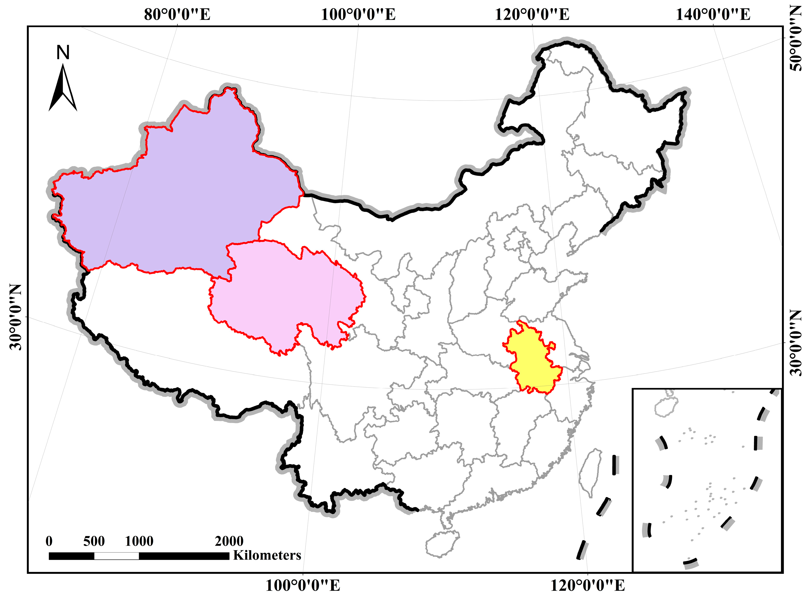
Figure 1. Experimental region of this study. The yellow area represents Anhui Province (Figure 2). The pink area represents Qinghai Province (Figure 3). The purple area represents Xinjiang Uygur autonomous region.
Remotesensing 16 00098 g001
Figure 2. Distribution of candidate sets in Anhui Province, China. The blue polygon represents the GF6 image, and the red line is the boundary of the Anhui Province, China.
Remotesensing 16 00098 g002
Figure 3. Distribution of candidate sets in Qinghai Province, China. The blue polygon represents the GF6 image, and the red line is the boundary of the Qinghai Province, China.
Remotesensing 16 00098 g003
Figure 4. Distribution of candidate sets in Xinjiang Uygur autonomous region, China. The blue polygon represents the GF6 image, and the red line is the boundary of the Xinjiang Uygur autonomous region, China.
Remotesensing 16 00098 g004
Figure 5. The solution process of the proposed optimization algorithm. The purple rectangle represents the region of interest. The image density indicates the number of images covered on each grid; the specific experimental results are found in Section 4.1.
Remotesensing 16 00098 g005
Figure 6. Schematics of the unit element and compulsory subset.
Remotesensing 16 00098 g006
Figure 7. Density distribution of image retrieval results for the Anhui dataset: (a) Candidate data, (b) Li et al.’s method [23], (c) greedy algorithm, and (d) DD-RSIRA. The color scale from blue to red indicates the number of overlapping remote sensing images covering different grids. (The black circle indicates the significant optimization of the proposed method. The purple frame represents the boundary of the experimental area.)
Remotesensing 16 00098 g007
Figure 8. Density distribution of image retrieval results for the Qinghai dataset: (a) Candidate data, (b) Li et al.’s method [23], (c) greedy algorithm, and (d) DD-RSIRA. The color scale from blue to red indicates the number of overlapping remote sensing images covering different grids. (The black circle indicates the significant optimization of the proposed method. The purple frame represents the boundary of the experimental area.)
Remotesensing 16 00098 g008
Figure 9. Density distribution of image retrieval results for the Xinjiang dataset: (a) Candidate data, (b) Li et al.’s method [23], (c) greedy algorithm, and (d) DD-RSIRA. The color scale from blue to red indicates the number of overlapping remote sensing images covering different grids. (The black circle indicates the significant optimization of the proposed method. The purple frame represents the boundary of the experimental area.)
Remotesensing 16 00098 g009
Figure 10. Distribution of the image cost for the different methods (Li et al. [23], greedy algorithm and DD-RSIRA).
Remotesensing 16 00098 g010
Table 1. Information on the satellite used.
ProjectParameters
Launch Time2 June 2018
Orbit TypeSun-synchronous Orbit
Orbital Altitude644.5472 km
Orbital Period97.4658 min
Regression Cycle41 days
Spatial ResolutionPanchromatic: 2 m, Multispectral: 8 m
Swath Width95 km
Quantified Value12 bits
Table 2. Comparison of different methods of assessing the distribution of results. The best values for the different metrics are highlighted in bold.
RegionMethodCountCRAIDRRUR
AnhuiCandidate data148100%3.99889%-
Li et al. [23]68100%2.25359%12%
Greedy Algorithm50100%1.62242%32%
DD-RSIRA48100%1.50214%36%
QinghaiCandidate data857100%6.161000%-
Li et al. [23]313100%2.64302%7%
Greedy Algorithm263100%2.08236%14%
DD-RSIRA240100%1.88205%22%
XinjiangCandidate data2222100%7.881160%-
Li et al. [23]644100%2.52263%7%
Greedy Algorithm531100%1.99198%16%
DD-RSIRA487100%1.84172%20%
Table 3. Box plot statistics for the different methods. The best values for the different metrics are highlighted in bold.
RegionMethodMinQ1Q2Q3Max
AnhuiLi et al.0.02910.16330.29160.35480.5791
Greedy Algorithm0.03920.15900.26910.34570.5791
DD-RSIRA0.03920.16210.26910.35210.5791
QinghaiLi et al.0.00740.22100.31010.40500.5959
Greedy Algorithm0.00740.20840.29860.38790.5959
DD-RSIRA0.00740.20730.29420.37040.5959
XinjiangLi et al.0.00200.14510.23560.30670.5408
Greedy algorithm0.00200.12010.21860.29300.5408
DD-RSIRA0.00200.11940.22330.29300.5408
Disclaimer/Publisher’s Note: The statements, opinions and data contained in all publications are solely those of the individual author(s) and contributor(s) and not of MDPI and/or the editor(s). MDPI and/or the editor(s) disclaim responsibility for any injury to people or property resulting from any ideas, methods, instructions or products referred to in the content.