A Point Cloud Segmentation Method for Dim and Cluttered Underground Tunnel Scenes Based on the Segment Anything Model

Abstract

In recent years, point cloud segmentation technology has increasingly played a pivotal role in tunnel construction and maintenance. Currently, traditional methods for segmenting point clouds in tunnel scenes often rely on a multitude of attribute information, including spatial distribution, color, normal vectors, intensity, and density. However, the underground tunnel scenes show greater complexity than road tunnel scenes, such as dim light, indistinct boundaries of tunnel walls, and disordered pipelines. Furthermore, issues pertaining to data quality, such as the lack of color information and insufficient annotated data, contribute to the subpar performance of conventional point cloud segmentation algorithms. To address this issue, a 3D point cloud segmentation framework specifically for underground tunnels is proposed based on the Segment Anything Model (SAM). This framework effectively leverages the generalization capability of the visual foundation model to automatically adapt to various scenes and perform efficient segmentation of tunnel point clouds. Specifically, the tunnel is first sliced along its direction on the tunnel line. Then, each sliced point cloud is projected onto a two-dimensional plane. Various projection methods and point cloud coloring techniques are employed to enhance SAM’s segmentation performance in images. Finally, the semantic segmentation of the entire underground tunnel is achieved by a small set of manually annotated semantic labels used as prompts in a progressive and recursive manner. The key feature of this method lies in its independence from model training, as it directly and efficiently addresses tunnel point cloud segmentation challenges by capitalizing on the generalization capability of foundation model. Comparative experiments against classical region growing algorithms and PointNet++ deep learning algorithms demonstrate the superior performance of our proposed algorithm.

1. Introduction

Point clouds are data generated by laser scanners, depth cameras, or other sensors, providing high-dimensional information about the environment or objects. Point cloud segmentation is a significant task in the fields of computer vision and machine learning.

With the rapid development of digital mine Information Technology construction, tunnel environments are increasingly being applied in various industries, including transportation infrastructure, water resource engineering, the energy sector, and urban infrastructure. In response to the demands of digitization and intelligent development, techniques such as terrestrial laser scanning (TLS) [1,2] and photogrammetry [3,4] are being employed to capture information about tunnel structures. Laser scanning, in particular, is well-suited for dark environments within tunnels as it does not require additional lighting during data collection. Numerous studies have explored the application of laser scanning in tunnels, including cross-section extraction [5,6], deformation measurement [7,8], and 3D reconstruction [9,10]. These studies rely on the segmentation of point cloud data into contour structures, serving as a crucial step for further analysis and research. In the domain of digital mining, point cloud segmentation serves as the fundamental basis for achieving a deeper understanding of point cloud data. It provides essential technical support for tasks in the realm of mining, including the geological modeling of mining areas, quantitative management of coal mine resources, deformation monitoring of mine tunnels, health status monitoring of mechanical equipment, and path planning of mine tunnels. As a result, the point cloud segmentation of tunnels has emerged as a critical process for the application of point cloud data in tunnel-related studies.

However, underground tunnel environments are much more complex than road tunnels. These underground environments used for mining may involve extreme conditions such as high temperatures; high humidity; dim light; and dusty, noisy, and intense vibrations, which can disrupt the normal functioning of conventional laser scanning equipment. Moreover, the presence of mud, pipes, wires, and other equipments within tunnels contributes to a cluttered distribution of objects, making it challenging to identify specific structures such as tunnel segments and gaps, thereby increasing the difficulty of data collection and point cloud segmentation in tunnels. Furthermore, the boundaries of tunnel walls may be indistinct, and the lighting conditions in tunnels are very poor, resulting in the inaccurate extraction of structural features, such as tunnel edges. Additionally, different tunnel scenes have unique characteristics, and the suitable public datasets for training segmentation models that can adapt to various tunnel environments are limited. These combined factors pose difficult challenges for the automation of point cloud segmentation.

In order to solve the aforementioned challenges, the paper proposes a method to segment dim and cluttered tunnel laser point cloud data, which means tunnel point cloud without RGB information and clear boundary information. The method leverages the zero-shot generalization capability of the pre-trained foundation model SAM [11] to achieve the arbitrary segmentation of tunnel-related 3D point clouds, thus providing fundamental methodological support for digitalization applications in tunnels. To summarize, our main contributions are as follows:

• Based on the zero-shot generalization capability of SAM, the study has formulated a framework for the semantic segmentation of 3D point clouds of complex underground tunnel scences. This framework demonstrates the automatic continuous segmentation ability of whole tunnel point clouds in complex scenes by utilizing point cloud slicing and label attribute transfer methods.
• Based on the prompt engineering capabilities of the SAM, our framework avoids additional training and does not depend on point cloud attributes like color and intensity. This framework optimizes the selection of front and back points required in the SAM prompt and controls the range of the segmented region by assigning different colors to pixels to improve the accuracy of tunnel point cloud segmentation.
• The study has conducted validation experiments involving 3D point cloud segmentation with complex settings, employing underground coal mine tunnels as an illustrative example. It is superior to traditional algorithms in both visualization and accuracy indicators. Consequently, the framework with good stability, flexibility, and scalability provides more ideas for point cloud segmentation in the development of foundation models.

2. Related Work

2.1. Semantic Segmentation of Point Clouds

Point clouds are widespread used in various domains, including computer vision, photogrammetry, and remote sensing [12]. Semantic segmentation in point clouds is applies to instance segmentation and panoramic segmentation. Before the advent of foundation models, common semantic segmentation methods were categorized into traditional algorithms based on geometric constraints and statistical rules, and fine-tuning deep learning algorithms relying on neural networks.

Traditional segmentation methods can be categorized into four main approaches: edge-based, region growing, model fitting, and clustering. Edge-based methods [13] focus on detecting rapid intensity changes in the point cloud and extracting closed contours from binary images to delineate boundaries between different regions [14]. These techniques are typically well-suited for initial point cloud segmentation and are particularly useful in relatively uncomplicated scenes. Model fitting methods, on the other hand, aim to align the point cloud with various primitive geometric shapes. Most commonly used algorithms include the Hough Transform (HT) and the Random Sample Consensus (RANSAC), as originally proposed by Fischler and Bolles. However, the applicability of these two algorithms is limited when dealing with complex scenes or objects with irregular shapes. Clustering-based methods revolve around situations where the point cloud shares similar geometric features, spectral features, or spatial distributions. Common methods in this category encompass K-means [15,16,17,18,19] and fuzzy clustering [16,20]. The presence of surrounding noise points can significantly affect the efficacy of clustering methods. Region-growing-based methods represent a classic and widely adopted technique in point cloud segmentation [21]. This approach involves the transformation of 3D point clouds into 2D images and segmentation based on pixel similarity [22]. With the widespread adoption of 3D region growing techniques, this method now takes into account various factors, including point cloud normal vectors, distances between points, and distances between points and planes, which significantly enhance the segmentation accuracy of region-growing algorithms [23,24,25]. Presently, this stands as one of the most extensively used methods among traditional point cloud segmentation algorithms. However, different seed points and growth rules must be configured to suit various scenes and semantic classifications.

Fine tuning deep learning algorithms for point cloud segmentation has become a topic of attention. They can generally be categorized into three classes: projection-based, voxel-based, and point-based. Projection-based techniques involve the projection of 3D point clouds onto a 2D plane. Su proposed a multi-view deep learning model known as MVCNN [26]. However, this algorithm sacrifices certain aspects of the spatial structure inherent in point clouds. Voxel-based methods were initially employed in deep learning-based point cloud semantic segmentation, combining voxels with 3D convolutional neural networks. The most renowned example of a voxel-based 3D CNN is VoxNet [27], but it is primarily suited for object detection. Building upon this method, the SegCloud framework was introduced, which initially voxelizes the original point cloud and then employs Fully Connected Neural Networks (FCNN) to generate downsampled voxel labels. Subsequently, these voxel labels are transformed into semantic labels for the 3D points. Nevertheless, this approach is constrained by the computational cost associated with voxel resolution and segmentation accuracy. Point-based algorithms for point cloud segmentation directly extract features from the point coordinate information. PointNet [28] was a pioneering work in this domain, and subsequently, local geometric information between point clouds was integrated into neural networks, leading to the widely adopted PointNet++ [29]. Numerous researchers have further enhanced PointNet++, with the design of an edge feature extractor being particularly noteworthy. They integrated edge convolution into neural networks, resulting in DGCNN [30], which further enhances the effectiveness of deep learning in point cloud segmentation. Deep learning algorithms impose stringent requirements on the quality of datasets, particularly in tunnel scences. The higher the quality of the dataset, the more superior the segmentation results achieved by the trained models.

With the emergence of foundation models, particularly the impressive performance of the Segment Anything Model (SAM), an increasing number of scholars have embarked on leveraging pre-trained large models for 3D point cloud segmentation. Yang harnessed SAM’s segmentation capabilities for RGB images to segment different views of a 3D scene into distinct masks [31]. Subsequently, they projected these 2D masks onto the 3D point cloud and, employing a bottom-up approach, amalgamated the 3D masks, thereby achieving fine-grained segmentation for 3D scenes. In a similar vein, Wang devised a method for projecting 3D point clouds onto 2D images [32]. This method preserves the geometric projection relationships and color perceptual capabilities of the images. Through analysis of the performance of various pre-trained models, they concluded that fine-tuning methods based on pre-trained models outperformed traditional fine-tuning deep learning methods. Inspired by these endeavors, the study leveraged the generalization capability of the foundation model, eliminating the need for training, to achieve semantic segmentation for undergound tunnel scenarios.

2.2. Point Cloud Segmentation in Tunnel

Due to the complex environment in the tunnel, dim lighting, unclear boundaries, and disorderly pipeline distribution, point cloud segmentation in tunnels poses greater challenges. Zhang proposed a circle projection algorithm to transfer 3D point clouds into 2D images [33]. The algorithm, which is based on Unet, can segment pipe, power track, cable, support, and track. Soilán applied the PointNet model and KPConv architectures to perform a multi-class classification, including ground, lining, wiring, and rails [34]. The two methods mentioned above are based on simple tunnel environment and point cloud data, which can leverage the performance of the algorithm. Ji proposed a data cleaning method and designed an encoder-decoder deep learning model [35]. However, this algorithm has a relatively complex neural network structure and requires training different models for different tunnel environments. To sum up, point cloud segmentation algorithms primarily find application in the extraction of tunnel feature lines, as well as the identification of specific structures and equipments in the tunnels.

In the context of tunnel feature line extraction, Ai acquired cross-sectional data from the original tunnel point cloud data by analyzing point cloud spatial geometry relationships [36]. They also harnessed the K-nearest neighbor calculation method to deduce the tunnel’s central axis. Meanwhile, Wang conducted a joint analysis with total-station-based surveying data, which was based on the acquisition of 3D laser point clouds [37]. Their approach showcased the ability to monitor the comprehensive deformation of the tunnel, demonstrating the utility of 3D laser scanners in tunnel structural monitoring. Li utilized tunnel laser point cloud data to approximate the tunnel centerline, the spatial coordinates of key locations, and equipment like cavern and anchor rods. These data were then integrated with Building Information Modeling (BIM) data to reconstruct a comprehensive 3D tunnel model [38].

Concerning the extraction of specific structures within the tunnel, Si employed an enhanced region-growing method to discern coal-rock layers [39]. Lu employed region segmentation and the random consensus algorithm and fine-tuned parameters to extract elliptical cylindrical surface models within the tunnel [40]. Liu proposed a multi-scale and multi-feature extraction technique for detecting water leakage on tunnel walls using point cloud intensity images [41]. His method integrated residual network modules into a cascaded structure, resulting in a unified model for extracting multi-scale features of water leakage. Du used noise-filtered tunnel point cloud data to implement an automated detection method for longitudinal seams, along with a swift large tunnel point cloud filtering method that accurately extracts tunnel lining walls and all longitudinal seams [42]. Farahani segmented the damaged areas on the tunnel wall that need to be repaired [43]. He combined cameras and LiDAR, focusing on using cameras for recognition and extraction, using point cloud data for localization and achieving the health monitoring of tunnels. Yi addressed the segmentation of colorless tunnel point cloud data and employed cross-sectional point cloud analysis to extract the boundaries of the tunnel [44]. However, this study specifically focused on circular tunnels, with a greater emphasis on segmenting the tunnel segments on the walls during the segmentation process. Zhang proposed an integrated segmentation model capable of effectively delineating various objects within large-scale three-dimensional tunnel point clouds, with a particular emphasis on achieving precise segmentation in the context of seepage flow [45]. This article innovatively projects points to a cylinder and utilizes 2DCNN to segment components such as power tracks, cables, and pipes within the tunnel. Park systematically compared two deep learning algorithms, PointNet++ and DGCNN, with a focus on adjusting algorithmic parameters to identify a configuration that better suits tunnel conditions [46].

The tunnel point cloud lacks datasets with semantic labels, and point cloud segmentation models trained on indoor 3D datasets, such as S3D [47] and Scannet [48], which have achieved a good general segmentation results. Xing demonstrated the viability of DGCNN in coal mine tunnel point cloud scenes and established a dataset tailored for coal mine tunnel point cloud segmentation [49]. This research culled data from the intersection between coal wall and the roof of the long-wall working face, offering inspiration for generating point cloud datasets and extracting other pertinent features.

Inspired by these studies, a more generalized framework is proposed in order to overcome challenges in underground tunnel scenarios, such as insufficient color information, high levels of equipment-related noise, and unclear boundaries. This framework addresses the difficulties posed by limited point cloud datasets in tunnel scenes and aims to achieve semantic segmentation for any class category within various tunnel scenes.

3. Methods

In the study, a method is proposed that leverages the zero-shot generalization capabilities of the foundation model SAM, as shown as Figure 1, for instance, the segmentation of tunnel 3D point cloud data. Initially, rotate and partition the entire tunnel point cloud data into numerous sliced subscenes. Subsequently, employ methods of parallel projection and perspective projection to project the 3D point cloud onto a two-dimensional plane. Then, utilize the image segmentation capabilities of SAM to perform pixel-wise segmentation on the projected images of each tunnel slice. By establishing correspondences between 3D point cloud data and 2D image pixels, labels are assigned to the 3D point cloud. The labeling information of the 3D point cloud is progressively transmitted, slice by slice, through overlapping regions of adjacent slices, ultimately resulting in a segmentation mask for the entire tunnel scene in 3D point cloud data.

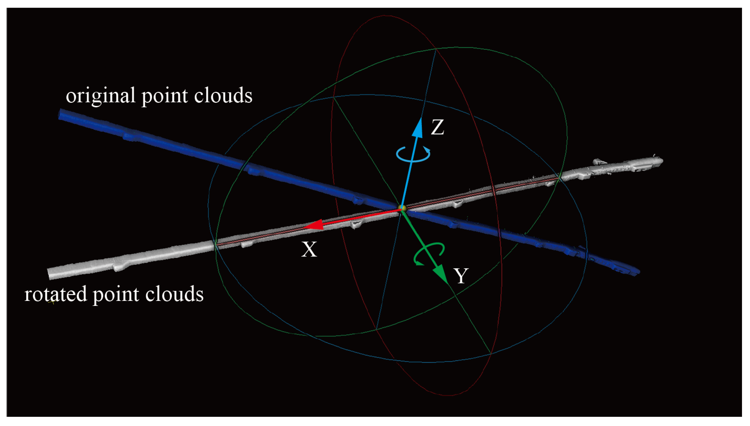
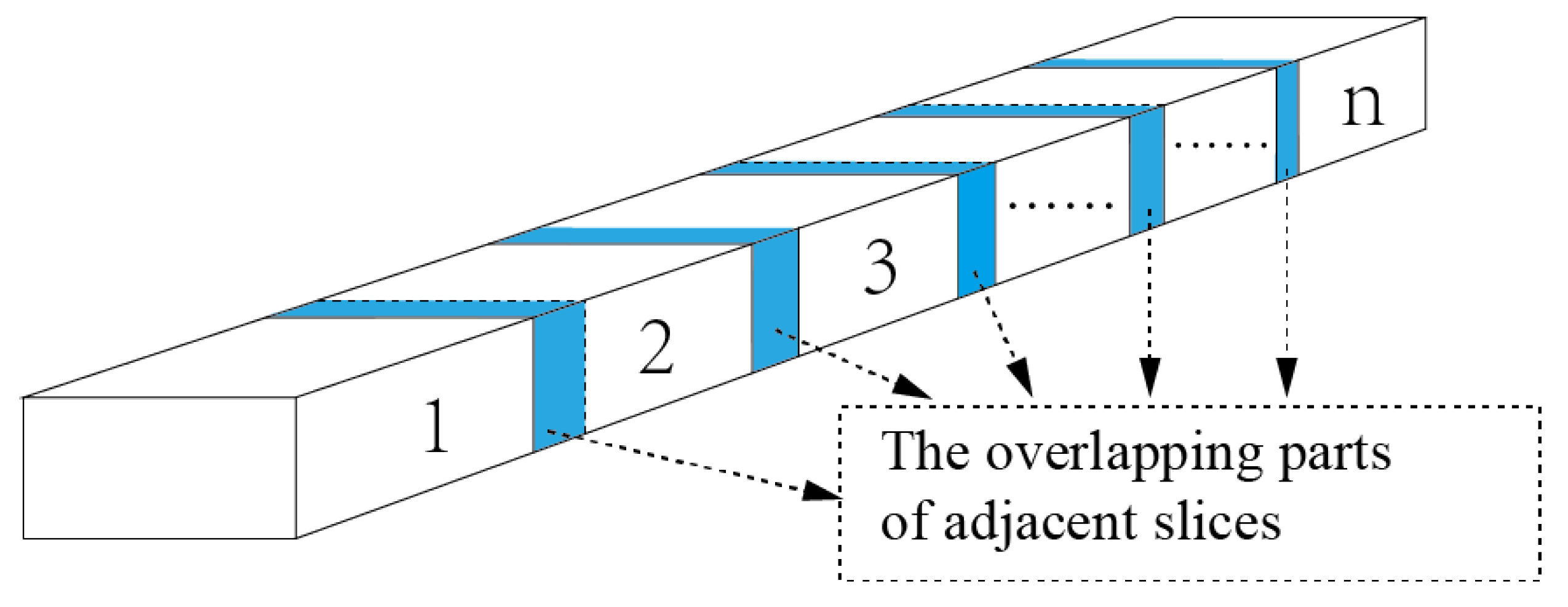
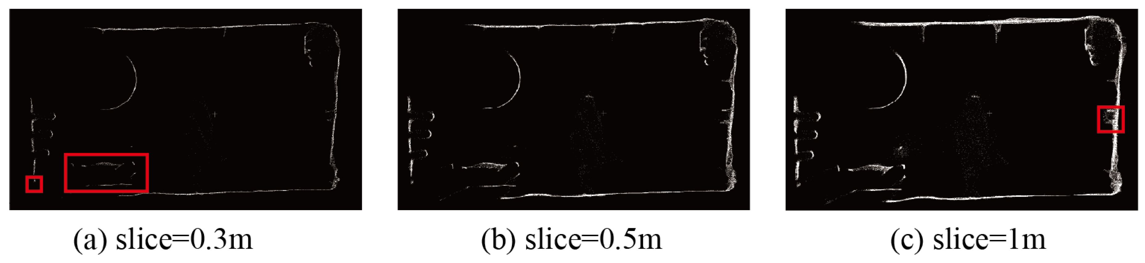
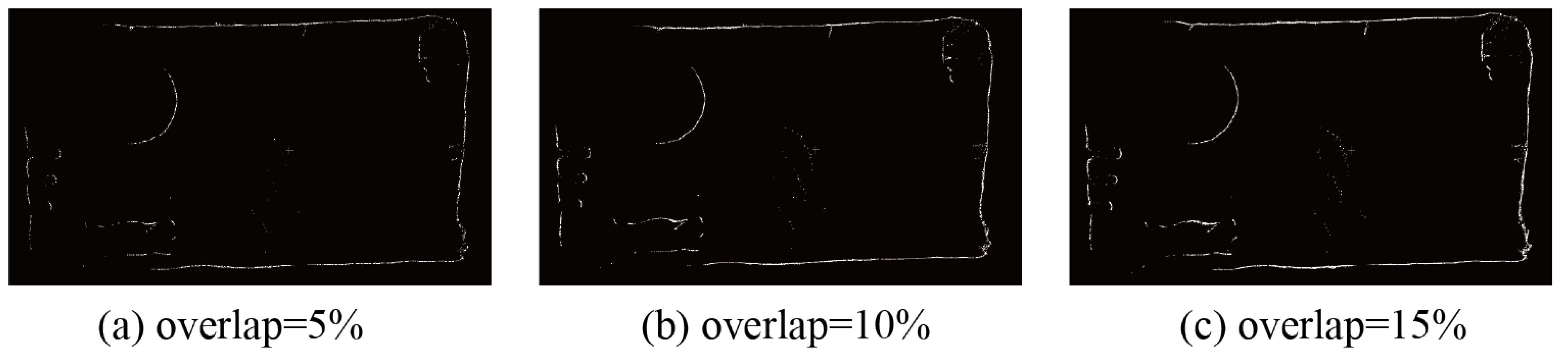
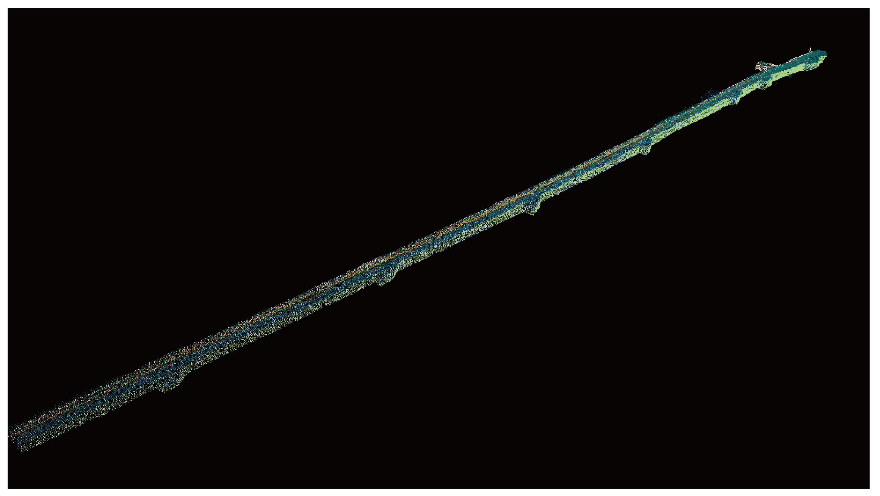
3.1. Point Cloud Rotation and Slicing

Point cloud rotation is a rigid transformation. Tunnel point cloud data are typically in voluminous and tend to be distributed along the tunnel direction. For convenience of calculation and processing, the tunnel’s overall direction is rotated to approximately align with the X-axis of the world coordinate system, as shown in Figure 2. The primary process consists of two steps:

• Calculating the tunnel’s direction by using Principal Component Analysis (PCA) [50] to linearly reduce the dimension of the entire tunnel point cloud and calculate its first principal component as the tunnel’s direction, $\overrightarrow{p_0}(x_0,y_0,z_0)$.
• Calculating the rotation matrix for the point cloud and applying a rotation transformation to all points. The rotation matrix is computed as shown in Equation (1); the point cloud is first rotated along the X-axis and then along the Y-axis, orienting it towards the X-axis direction.

$$pointclou{d}^{\prime }=matri{x}^Y\ast matri{x}^Z\ast pointcloud$$

(1)

$$matri{x}^Z=\left[\begin{array}{ccc}0& 0& 1\\ 0& cos\left(arctan(y_0/x_0)\right)& -sin(arctan(y_0/x_0)\\ 0& sin\left(arctan(y_0/x_0)\right)& cos\left(arctan(y_0/x_0)\right)\end{array}\right]$$

(2)

$$matri{x}^Y=\left[\begin{array}{ccc}cos\left(arctan(\sqrt{y_0^2+z_0^2}/x_0)\right)& 0& sin(arctan(\sqrt{y_0^2+z_0^2}/x_0)\\ 0& 1& 0\\ -sin\left(arctan(\sqrt{y_0^2+z_0^2}/x_0)\right)& 0& cos\left(arctan(\sqrt{y_0^2+z_0^2}/x_0)\right)\end{array}\right]$$

(3)

Point cloud slicing refers to the process of segmenting and slicing a target point cloud along a specific direction using a series of mutually parallel and evenly spaced planes. The key aspect of this method lies in determining the cutting direction and thickness of the point cloud slices. Different slicing directions result in variations in the resulting planar point clouds. When performing slicing, the cutting direction should be determined based on the shape and structural characteristics of the point cloud. In this study, based on the rotation of point cloud coordinates, the slicing was conducted in the direction perpendicular to the X-axis, which corresponds to the direction of the tunnel. This was achieved by using specific interval planes to slice the target point cloud. The thickness of the point cloud slices plays a crucial role in determining the precision of subsequent point cloud segmentation. A larger thickness results in more noise around the target point cloud to be segmented, while a smaller thickness may hinder the perspective representation of the segmented target point cloud, both of which can impact the effectiveness of point cloud segmentation. In this study, different slicing intervals were set based on the situation. When using parallel projection for 2D to 3D transformation, the tunnel slicing intervals were set as small as possible, whereas for perspective projection in 2D to 3D transformation, intervals needed to be set to increase because to express spatial relationships of point clouds with small intervals.

When employing the SAM for the automatically segment whole tunnel point clouds, it is essential to ensure the overlapping points between adjacent slices of the point cloud. As illustrated in Figure 3, the tunnel’s point cloud is segmented into n slices, each of which includes parts of adjacent part data.

3.2. Mapping 3D Point Clouds into 2D Images

Projecting 3D point clouds onto a 2D plane is a fundamental spatial data processing technique. This projection procedure effectively keeps the core shape and structure of the point cloud, thereby enhancing its accessibility for analytical, visualization, and processing purposes. Based on the method, the 3D coordinates $(X,Y,Z)$ of each point are correspondingly mapped to coordinates $(U,V)$ on the 2D plane while preserving other attributes associated with the points, such as color and intensity. Such a projection can be achieved by various mathematical methodologies, including perspective projection and parallel projection.

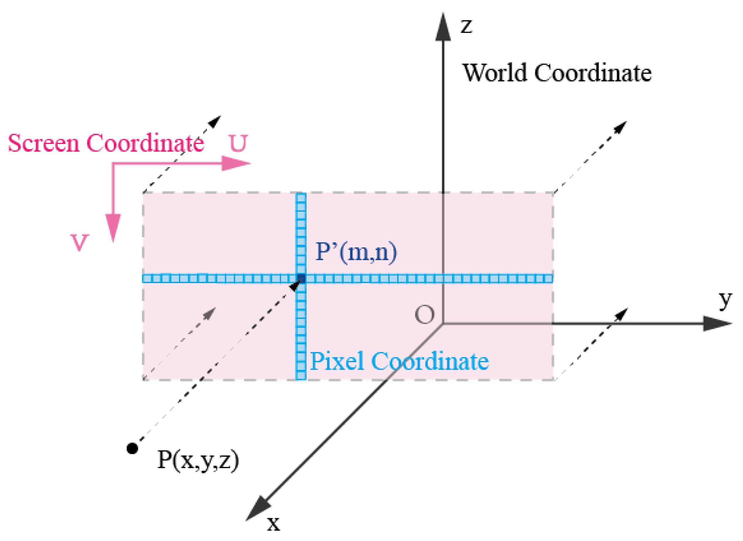
3.2.1. Parallel Projection

The concept of parallel projection is fundamentally straightforward. It involves simulating rays originating from an infinitely distant point source directed towards an object. Subsequently, it records the positions of these projected points on a plane that is parallel to the projection plane, effectively creating an image. The defining characteristic of parallel projection is that it projects all points along the same direction, and the position of a point on the projection plane is determined solely by its projected position in that direction and its location on the projection plane. Consequently, parallel projection preserves the original shape of the point cloud and maps these points from 3D points to 2D plane, thereby reducing the data’s dimension. It is essential to emphasize that parallel projection may result in overlapping points, particularly between those that are close and those that are distant. Consequently, the thickness of the slices and the direction of the projection directly influence the quality of the resulting 2D image and the accuracy of the final segmentation. The process of converting 3D coordinates into a parallel projection 2D image is visually depicted in Figure 4 and can be broken down into several key steps.

• Select Projection Plane: After the tunnel slice processing in the previous section, for each slice, choose the slice with the maximum X-coordinate as the target plane for projection, with the tunnel’s direction as the projection direction.
• Determine the Plane Coordinate System: Calculate the minimum bounding box for each 3D point cloud slice, find the maximum and minimum values in the Y and Z directions, namely, $y_{min},y_{max},z_{min},z_{max}$. Take $(y_{min},z_{max})$ as the origin of the plane and transform the 3D coordinates of the point cloud in the slice into 2D coordinates on the plane, where points are marked as $P_{UV}=(\frac{y-y_{min}}{y_{max}-y_{min}},\frac{z_{max}-z}{y_{max}-y_{min}})$.
• Generate Projection Images: Use $w=y_{max}-y_{min}$ and $h=z_{max}-z_{min}$ as the width and height of the image on the projection plane, respectively. Based on the desired image resolution $m\times n$, divide the plane into grids and then convert each point in the slice into pixel coordinates on the image. The points in pixel coordinates are marked as $P_{pix}=(\frac{u\times m}{w},\frac{v\times n}{h})$

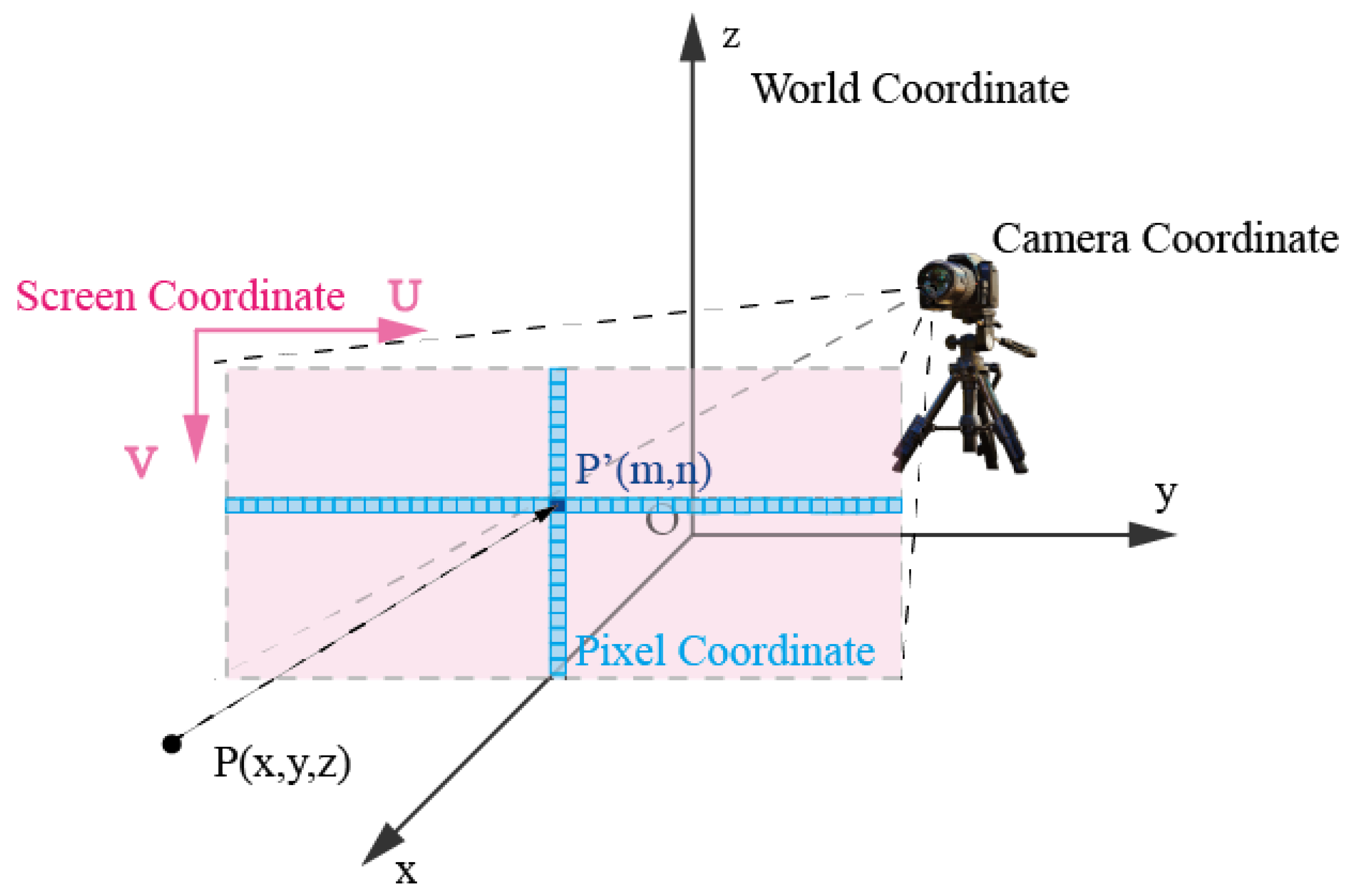
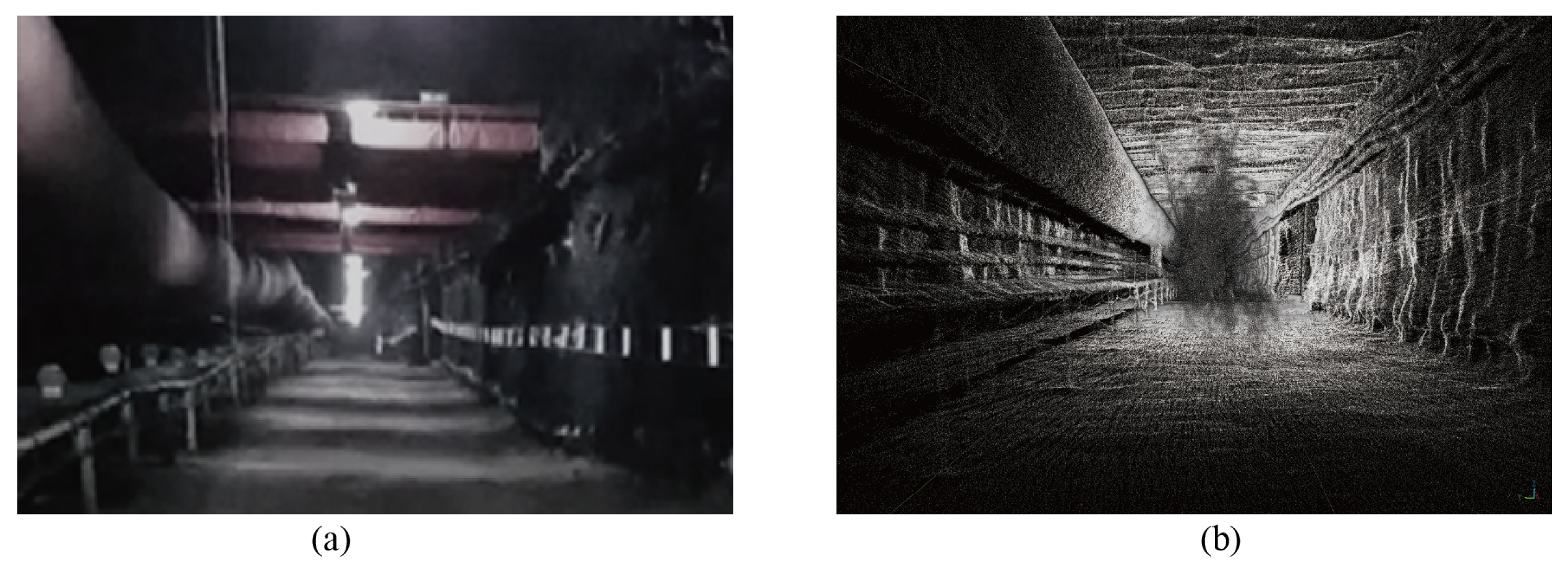
3.2.2. Perspective Projection

Perspective projection constitutes a technique used to project 3D objects or point cloud data onto a 2D plane, effectively emulating the effects of human perspective vision. This process aims to render the projection in a manner that closely approximates what the human eye perceives as a faithful representation of the actual scene. The fundamental underpinning of perspective projection involves a combination of spatial coordinate transformations and optical concepts. In stark contrast to parallel projection, this method accounts for the spatial relationship between each point and the observer. This unique approach results in points that are closer to the observer and appear larger in the projection, while those situated farther from the observer appear smaller. This deliberate manipulation achieves a more lifelike and realistic visual effect. As illustrated in Figure 5, the projection plane clearly demonstrates this phenomenon: the blue plane, which is closer to the observation plane, appears to be notably larger in the final projected image compared to the red plane, positioned at a greater distance. The below elucidates the foundational principles and sequential steps involved in perspective projection.

• Selecting the Viewpoint:In perspective projection, it is necessary to determine the observer’s viewpoint, which is the observer’s eyes. This article uniformly sets the observation distance d and calculates the minimum bounding box and coordinate center $P_{center}(x_{center},y_{center},z_{center})$ for each slice. The viewpoint for each slice is placed at a distance d from the coordinate center towards the negative x-axis, which is marked as $P_{viewPoint}(x_{center}-d,y_{center},z_{center})$.
• Selecting Projection Lines: Projection lines refer to the lines that pass through the point cloud points from the viewpoint and intersect the projection plane vertically. By varying the endpoint positions of the projection lines, a greater number of perspective projection effect diagrams can be obtained. In the paper, the central projection line is used as an illustrative example. The center projection line starts from the center point of the slice with the smallest x-coordinate $V_{view}=(P_{viewPoint}-P_{center})$.
• Selecting the Projection Plane: Once the projection lines and viewpoint are determined, a projection plane is generated at a distance f from the viewpoint, perpendicular to the direction of the projection lines.
• Calculating Projection Points: Displaying the 3D point cloud in the projection plane. Firstly, the 3D point cloud in the original spatial coordinate system is transformed to have the viewpoint as the new coordinate system’s origin, with one axis as the direction of the projection lines. The homogeneous coordinates of the original point cloud are marked as $P{C}_{n\times 4}$, and the homogeneous coordinates of the point cloud under the new coordinates are represented as $P{C}_{n\times 4}^{\prime }=P{C}_{n\times 4}·R{T}_{4\times 4}$, where $R{T}_{4\times 4}$ is calculated in Equation (4), $R_{3\times 3}=[{[[0,0,1]\times V_{view}]}^T,{[0,0,1]}^T,-V_{view}^T]$, $T_{1\times 3}=-P_{viewPoint}$

  $$R{T}_{4\times 4}=\left[\begin{array}{cc}{R}_{3\times 3}& 0\\ T_{1\times 3}& 1\end{array}\right]$$

  (4)
  Secondly, the 3D coordinates in the new coordinate system are transformed into the 2D coordinate system of the projection plane to calculate the perspective projection coordinates of each point in 3D space on the projection plane. The points in the projection plane are marked as $P_{UV}=(\frac{f\times P{C}_x^{\prime }}{P{C}_z^{\prime }},\frac{f\times P{C}_y^{\prime }}{P{C}_z^{\prime }})$.
• Generating the Point Cloud Perspective Projection Image: Calculate the minimum bounding box of the projection points on the projection plane, based on the desired image resolution. The method is similar to the one mentioned in Section 3.2.1.

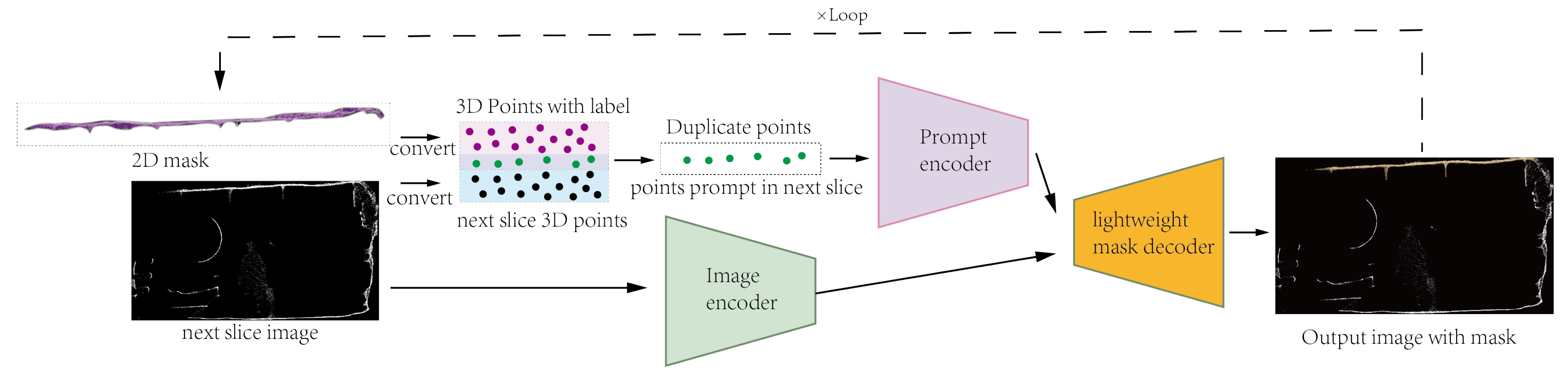
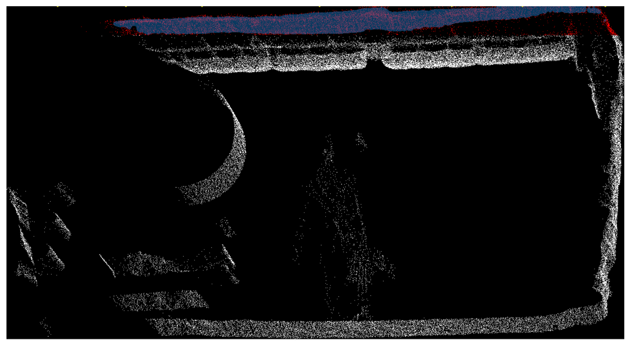
3.3. Using SAM to Generate a Single 3D Mask

In our study, a series of essential procedures was conducted to analyze the tunnel point cloud data. First, all of the point cloud datasets were segmented, and the initial sliced image along the x-axis direction was subsequently extracted. These single frame images were then subject to manual annotation using the SAM to produce the requisite pixel-level image masks. As is shown in Figure 6, some roof points in first slice image were selected as the SAM prompt to label some roof points in 3D with a roof mask. Subsequent to generating the 2D image in the preceding step and manually selecting foreground points, the image and associated cues were encoded, and this information was fed into the SAM model. The SAM model, in turn, promptly generated multiple segmented masks in accordance with the provided cues. For the given prompt, SAM model outputs three masks. In practice, it can generate more segmentation results, but for most cases, three masks suffice to represent the entirety, parts, and subparts of an object. During back propagation, only the parameters associated with the mask that minimizes the loss are involved in the computation. The study employs the IOU metric to rank the masks and select the one with the highest IOU, surpassing 90%, as the final point cloud label that meets our requirements. These masks were subsequently decoded and overlaid onto the 2D image. Finally, through the continuous adjustment of cue points guided by prior knowledge, the precise segmentation of 2D images with accompanying masks was achieved.

Following the acquisition of the pixel-level image masks, the study employed a coordinate transformation matrix to derive a classification mask encompassing the 3D point cloud, thereby facilitating semantic labeling of the initial 3D sliced point cloud. This coordinate transformation entailed conversions between various coordinate systems: world coordinates, camera coordinates, plane coordinates, and pixel coordinates.

Equation (5) shows the conversion of screen coordinates to pixel coordinates. Equation (6) shows the conversion of camera coordinates to screen coordinates conversion. Equation (7) shows the conversion of world coordinates to camera coordinates conversion.

$$(P_x,P_y)=([\frac{U·re{s}_U}{U_{max}-U_{min}}],[\frac{V·re{s}_V}{V_{max}-V_{min}}])$$

(5)

$P_x$ and $P_y$ denote pixel coordinates, U and V represent 2D plane coordinates, and $re{s}_U$ and $re{s}_V$ correspond to the image’s width and height resolutions.

$$(U,V)=(\frac{x_C·f}{z_C},\frac{y_C·f}{z_C})$$

(6)

$x_C,y_C,z_C$ denote the coordinates in the camera coordinate system, while f represents the distance from the viewpoint to the projection plane.

$$(x_C,y_C,z_C)=((x_W,y_W,z_W)-P_{viewPoint})·R_{3\times 3}$$

(7)

$x_W,y_W,z_W$ are the coordinates of the point cloud in the world coordinate system, while $R_{3\times 3}=({\left(righ{t}_{dir}\right)}^T,{\left(u{p}_{dir}\right)}^T,{\left(vie{w}_{dir}\right)}^T)$ represents represents the rotation matrix converted from world coordinates to camera coordinates.

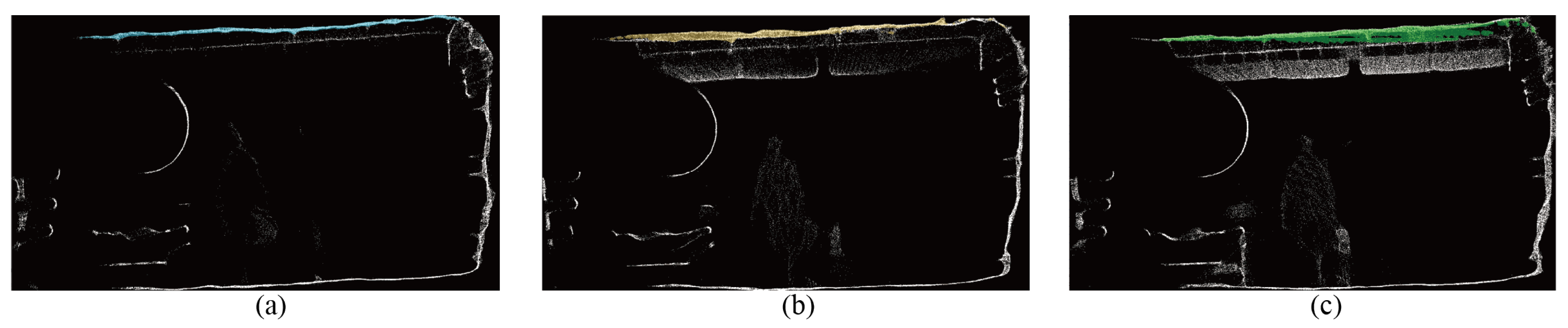
3.4. Automatically Generate 3D Masks for Whole Tunnel

In the preceding section, the paper presented a method for segmenting singel 3D point cloud slices using the SAM. This technique is introduced through building upon this, a recursive segmentation. To elaborate, the point clouds are derived from two consecutive slices represented as $X_1=x_{11},x_{12},\dots ,x_{1m}$ and $X_2=x_{21},x_{22},\dots ,x_{2n}$, where m and n denote the numbers of points in $X_1{X}_2$, respectively. To ensure a certain degree of overlap between the point clouds of adjacent slices when processing the entire point cloud datasets of a tunnel, $x_{1m-p},x_{1m-p+1},\dots ,x_{1m}=x_{21},x_{22},\dots ,x_{2p}$. The segmentation mask discussed in the previous section is employed, and it is recursively passed to the subsequent slice. Subsequently, the points are input as a prompt into the SAM model to predict the mask for the $X_2$ slice. During this step, the point cloud labels from the transmitted $X_2$ slice are arranged, and ten points are selected as prompts for the SAM model to prevent excessive segmentation. As shown in Figure 7, the previous image generates point clouds with semantic labels, and after an automated filtration process, prompt points that can be utilized for the next image. After that, a mask is yielded by SAM when both the subsequent image and the automatically generated prompt points are input. This obtained mask, along with the prompt points, is then reintroduced into SAM to derive a more precise 2D image with a mask. By employing this method, the properties of the 3D point cloud are recursively utilized to provide prompts to the SAM model, thereby achieving semantic segmentation of the entire tunnel point cloud.

4. Experiment

4.1. Data and Experimental Environment

To validate the research approach mentioned previously, the paper conducted experimental research within a specific underground coal mine conveyor tunnel. This tunnel is equipped with substantial belt conveyors and ventilation equipments. The experimental site spans approximately $342\mathrm{m}$ in length, featuring a rectangular cross-section with net dimensions of about $5.8\mathrm{m}$ in width and $2.86\mathrm{m}$ in height, resulting in a cross-sectional area of $16.59{\mathrm{m}}^2$. The data conform to point cloud data in complex environments. The environment of the tunnel can be found in Figure 8a. The study used the digital LiGrip H120 handheld laser scanning system (GreenValley International, Berkeley, CA, USA) to gather point cloud data, capable of capturing data in ${280}^{\circ }\times {360}^{\circ }$ direction. The laser scanning system’s parameters are detailed in

Table 1. LiGrip H120 Lidar system parameters.

Parameters	Data
Handheld size	L204 mm × W130 mm × H385 mm
Handheld weight	1.74 kg
Scanning field of view	280° × 360°
LiDAR accuracy	±3 cm
Point frequency	320,000 pts/s

. To enhance the algorithm’s adaptability and better suit it for the dimly light environment of the mining site, the study utilized colorless point cloud data, as illustrated in Figure 8b.

With the aid of LiFuser-BP version 1.5.1 and LiDAR360 Version 6.0, alongside the SLAM algorithm, the study expediently procured high-precision 3D point cloud data through scanning. The point cloud data collected during the experiment are stored in the PLY format, including spatial coordinates $X,Y,Z$ and the reflection intensity of the tunnel. A total of 32,179,432 data points are recorded, resulting in a data size of approximately 2.2 GB. Our experimental setup comprises a server computer equipped with an 8-core Intel(R) Gold 6234 CPU @ 3.30 GHz and one NVIDIA GeForce RTX 3090 GPU.

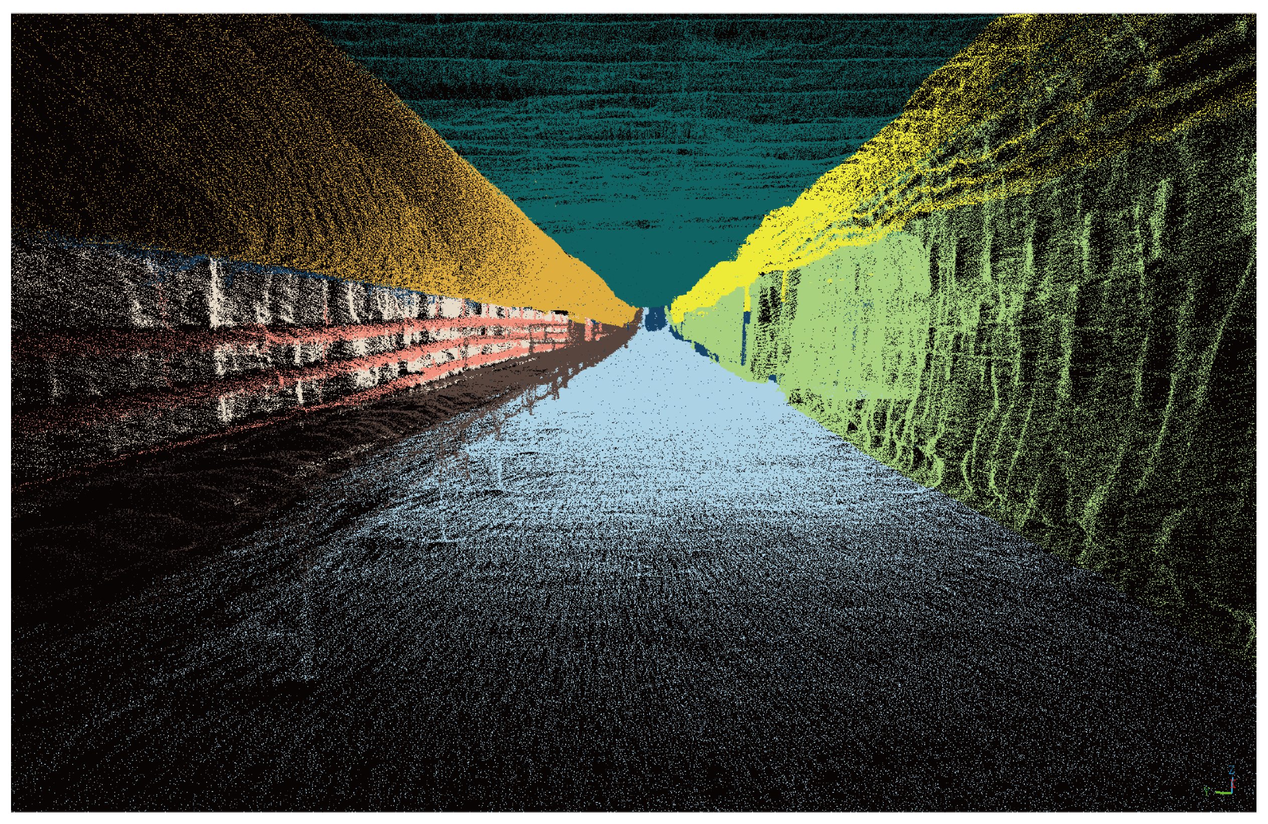
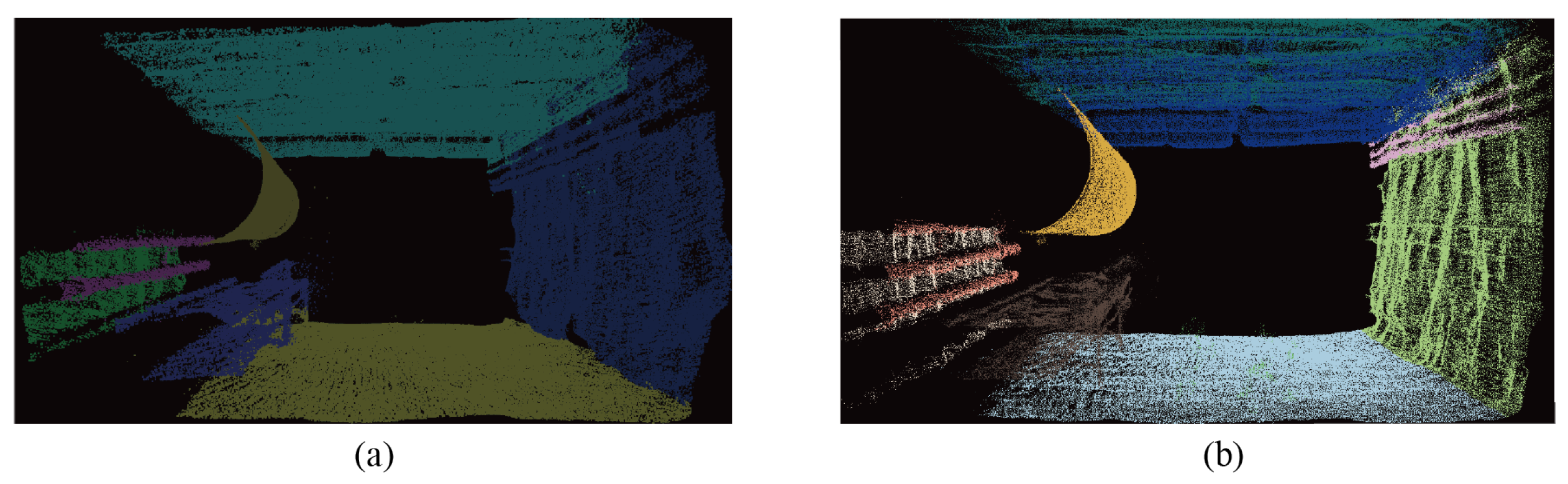
4.2. Result of Semantic Segmentation

The underground coal mine tunnel environment is complex, and there is a lot of point cloud noise in the tunnel. The paper divides the entire tunnel into seven categories of point clouds: left wall, roof, right wall, floor, belts transport, air duct, and wires. Due to the strong repetitiveness of the entire tunnel in the direction, this paper mainly uses the method of parallel projection to convert the 3D point cloud slices of each tunnel into 2D plane images. Here, the study conducted various experiments, converting point cloud slices into 2D depth maps and gray images with intensity information. It is found that the SAM model is more sensitive to the RGB color information of the images. Under the projection method used in this paper, converting depth and intensity information into RGB values will lower the effectiveness of SAM segmentation. Therefore, the study set all the projected images to binary images.

The thickness of the tunnel slices decides the image quality. When the slice thickness is too small, such as 0.3 m, the point cloud projection image exhibits an overly sparse concentration. During image segmentation using SAM, there is a risk of under-segmentation, leading to the inability to separate points of the same type, as indicated by the red box in Figure 9a. On the other hand, when the slice thickness is too large, such as 1 m, there is a higher concentration of noise points around the tunnel walls. When using SAM to segment the point cloud projection image, there is a tendency to misclassify noise points as the desired point cloud category, as illustrated by the red box in Figure 9c. Therefore, in this study, the point cloud slice thickness is set to 0.5 m, as shown in Figure 9b.

When setting the overlap rate, in order to facilitate the automatic propagation of point cloud labels during tunnel slicing, it is necessary to introduce a certain level of point repetition. In this study, different parameters were tested, and a repetition rate of 10% was chosen for the slicing process, as is shown in Figure 10. An overlapping rate of 5% was found to be too small, leading to the disappearance of labeled points during the label propagation process and resulting in the failure of the entire tunnel segmentation. Conversely, a overlapping rate of 15% increased the computational overhead of the algorithm, causing a 15% increase in the number of tunnel slices. Furthermore, when converting pixels labeled by SAM into point cloud labels, the time complexity also increased. This study opted for a 10% overlapping rate to ensure the smooth propagation of labels while minimizing computational costs.

The different categories of point clouds after SAM segmentation are shown in Figure 11; these images are tunnel slices, 2D parallel projection images perpendicular to the tunnel axis, and different colored areas in the images represent different category masks.

A fully automatic point cloud semantic segmentation was achieved through the slicing method that was designed and the point cloud labeling propagation method that was used. The final results are as shown in Figure 12 and Figure 13, where Figure 12 is an overview image of the tunnel, and Figure 13 is an internal perspective view of the tunnel.

During the experiments, the study proposed a method that uses quantity statistics to color the point cloud to improve the SAM segmentation effect. When segmenting the roof point cloud border, due to noises such as hanging wires, lamps, and signs on the roof, the SAM model may incorrectly segment the surrounding noise as part of the roof. Therefore, the study proposed a method that uses the quantity of statistics of the point cloud to select the roof’s point cloud, allowing for point cloud data preprocessing. Because SAM is sensitive to image colors, the selected points within the range were colored by us, and more accurate points masks were predicted through points labeling propagation.

The proposed statistical method for quantifying point clouds entails projecting them onto a 2D plane and subsequently enumerating the point clouds within each row of pixels along the vertical axis of the image. As illustrated in Figure 14, the first red point from the left denotes the initial peak, signifying the horizontal position within the image with the highest point cloud density on the roof. Nevertheless, the thickness of the roof’s point cloud in the image pixels remains indeterminate. Consequently, the tunnel roof’s location is at all points preceding the first green point (The first trough of wave) in Figure 14. Subsequently, these selected points are labeled by color, as shown in Figure 15. The pixels corresponding to the roof’s point cloud are identified in red, while the blue region in the image represents the roof mask forecasted by the SAM. Ultimately, by exploiting the SAM model’s color sensitivity, the impact of noise around the roof was effectively reduced and the precision of the segmentation has been improved. Figure 16 displays the segmentation outcomes for the roof’s point clouds in various cross-sectional scences.

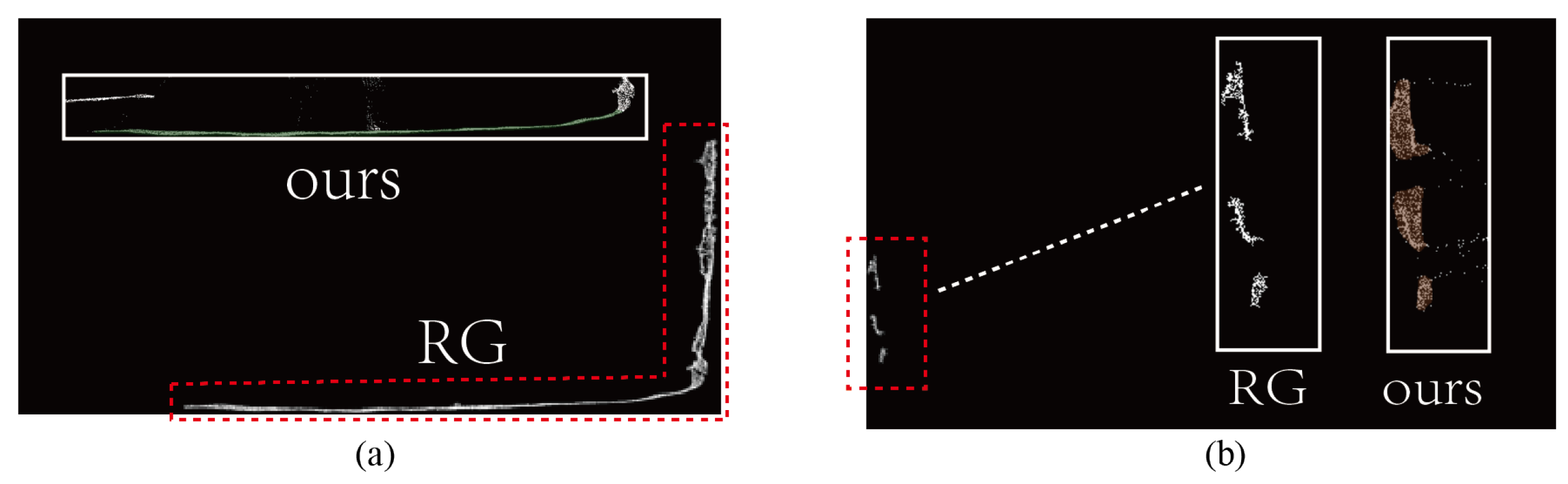
4.3. Comparative Experiment

In order to validate the performance of the algorithm, comparative experiments were conducted using two approaches: the traditional region-growing algorithm a nd the classic deep learning algorithm, PointNet++. The region-growing algorithm is a fundamental and widely applicable image segmentation technique. This algorithm iteratively expands regions by absorbing neighboring pixels based on their similarity until the growth process stops. Given that the point cloud projection of tunnel data results in a binary image with clear distinctions, seed points and pixel values were utilized as the criteria for similarity measurement to segment different classes. Segmentation experiments were conducted on seven different semantic categories within the tunnel, employing an 8-neighbor approach. PointNet++ is one of the common and high-performance segmentation algorithms in the field of deep learning. Due to the strong inherent spatial similarities along the tunnel slices in the direction of extension, this algorithm is capable of directly learning the distribution characteristics of points in three-dimensional space. By employing a well-trained model, it can effectively segment point clouds into different classes. Initially, the entire tunnel data was manually annotated by us, and then, with a slice thickness of 5 m, the entire tunnel was divided into 70 slices. The first 56 slices were used as the training dataset for the model, while the remaining 24 slices served as the testing dataset to evaluate the segmentation performance of the PointNet++ algorithm.

In the experiment, the study employed the Intersection over Union (IOU) score and precision as metrics for assessing segmentation performance, precisely defined as the ratio of the intersection to the union of “predicted results” and “ground truth”. In the case of perfect overlap, this ratio equals 1. The study conducted tests on the same set of 10 point cloud slices, yielding average segmentation metrics for various categories under different scenarios, as shown in

Table 2. Comparison of Ours to Region Growing and PointNet++.

	mIoU	Left Wall	Right Wall	Roof	Floor	Wires	Belts Transport	Air Tube
RG [21]	IOU	0.6145	0.4513	0.9198	0.3881	0.9408	0.5590	0.9878
	Precision	0.7362	0.5084	0.9312	0.5068	0.9574	0.7053	0.9912
PN [29]	IOU	0.8756	0.8940	0.9467	0.3728	0.0923	0.5136	0.8883
	Precision	0.9031	0.9215	0.9534	0.5041	0.1487	0.6675	0.9152
Ours	IOU	0.8774	0.7520	0.8217	0.9852	0.9554	0.7262	0.9958
	Precision	0.8923	0.7741	0.8389	0.9961	0.9721	0.7513	0.9971

. Our algorithm presents a competitive advantage over the Region Growing and PointNet++ algorithms in terms of the mIoU metric while also demonstrating strong performance in categories such as left wall, floor, wires, conveyor belts, and air duct.

The study further conducted visualizations of three algorithms. Firstly, the region growing method was compared with our algorithm, with a focus on the segmentation results for the base and left sidewall. Figure 17 illustrates the comparative results between our method and the region growing method. In Figure 17a, it is evident that the region growing method fails to accurately distinguish between the floor and right wall, whereas our algorithm accurately identifies the boundary between the floor and right wall. Figure 17b clearly shows that the region growing method results in a lower number of segmented points for the left sidewall compared to the original point cloud, while our algorithm effectively removes surrounding noise points and segments the complete left sidewall.

Secondly, the study compared the PointNet++ algorithm. As shown in Figure 18, our method is capable of performing semantic segmentation on complex tunnels and categories within the tunnels without training. Our algorithm effectively segments the walls, roof, and floor within the tunnel and is able to accurately segment small objects such as wires inside the tunnel and supports on the ceiling.

The study has analyzed the reasons behind the inferior performance of our algorithm compared to the PointNet++ algorithm in the segmentation metrics for the roof and right wall. From a parallel projection standpoint, the segmentation results for the roof and the right wall category appear relatively average, primarily due to increased noise at the junction of the roof and the right wall. The multi perspective perspective projection method helps to segment the edges between different categories of tunnel point clouds. Therefore, the segmentation effect of SAM in multiple perspectives is shown in the Figure 19. The left and right images are perspective projection images from different perspectives of the same slice scene. The colors represent the roof mask automatically predicted by the SAM model, and it is clear that the roof’s edges are well defined. In terms of the IOU metric, as depicted in

Table 3. Comparison of various perspectives and PointNet++.

	Indicator	Right Wall	Roof
pointnet++	IOU	0.8940	0.9467
	Precision	0.9215	0.9534
ours-view 1	IOU	0.9124	0.9552
	Precision	0.9238	0.9718
ours-view 2	IOU	0.9086	0.9485
	Precision	0.9234	0.9633

, superior ceiling segmentation performance has been achieved by explicitly refining the edges, surpassing the performance of PointNet++.

In the experiments, it is found that our method has a certain corrective effect on labeled datasets. When manually labeling data, errors and omissions are inevitable, as shown in Figure 20a, where the brown point cloud represents the manually labeled belts transport, which clearly does not include the entire belts transport, only marking the belt’s surface. However, the belts transport segmented by our method, as shown in Figure 20b, with the red point cloud, relatively comprehensively labels a part of the entire belts transport. Therefore, our proposed method demonstrates strong generalization for creating 3D point cloud labeled datasets in complex environments.

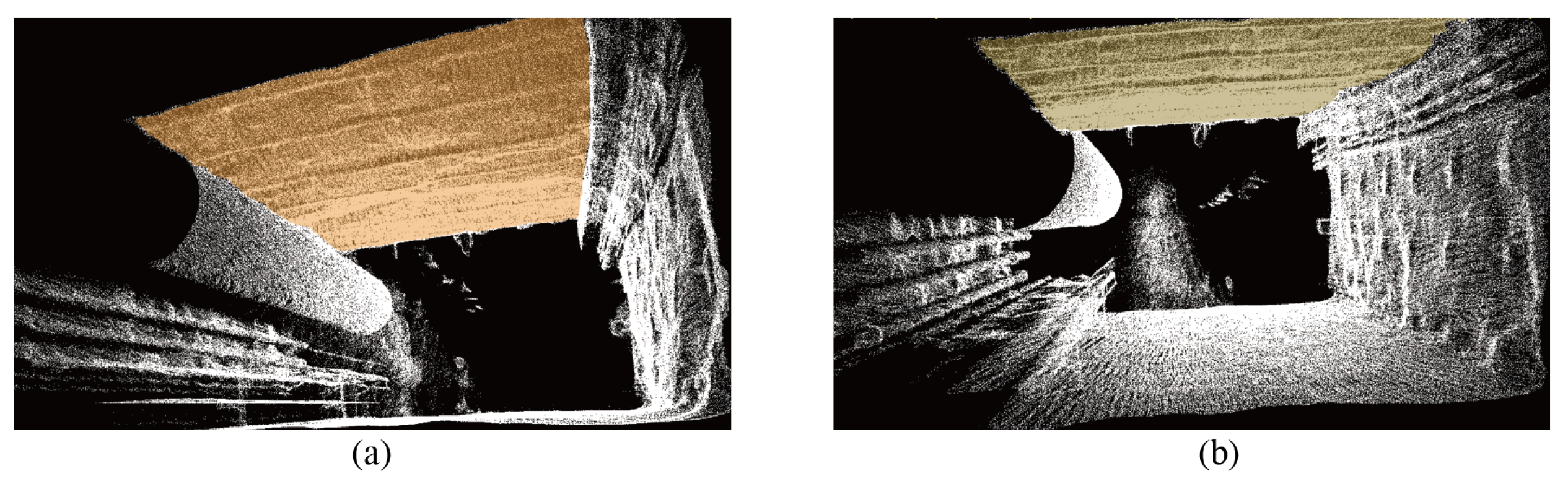
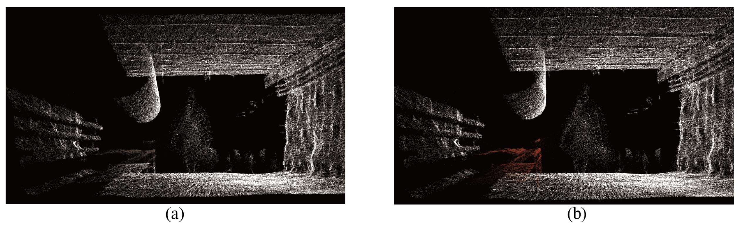
4.4. Scalability Experiment

This article further investigates the scalability of the proposed method in non-linear and different tunnel environments. For non-linear tunnels, the paper analyzes tunnel chambers within the dataset. As illustrated in the Figure 21, tunnel chambers are connected to tunnel walls and exhibit a natural tendency to curve. Slices taken at chamber locations, as shown in the Figure 21, reveal similar parallel projection patterns in point clouds. The method proposed in this paper can effectively segment point clouds at turning points, as demonstrated by the ability to capture complete representations of such turning locations.

For different tunnels, this paper employs the proposed method to segment point cloud data from a different tunnel, yielding favorable outcomes. The segmentation effect of a section in the tunnel is shown in the Figure 22. Figure 22a shows the point cloud data collected in Wuzhong, Ningxia Province. Figure 22b shows the point cloud data collected in Taiyuan, Shanxi Province. Figure 22c shows the point cloud data collected in Yulin, Shaanxi Province. The point clouds of different colors represent the floor, roof, left wall, right wall, air tube, and wires in different tunnels.

5. Discussion and Conclusions

This study presents a novel approach to point cloud segmentation in dim and complex conditions, such as underground coal mines. The method can transform 3D points into 2D pixels. This method leverages the SAM model to accurately comprehend tunnel point cloud scenes and perform semantic segmentation tasks. Simultaneously, the study employs the manual annotation of the first frame image and utilizes the similar attributes along the extension direction of the tunnel to automatically propagate the label properties of the point cloud, achieving fully automatic point cloud segmentation for the entire tunnel. In comparison with prevailing methods for the semantic segmentation of tunnel point clouds, this approach improves the accuracy of point cloud recognition and reduces the training cost of point cloud segmentation. Notably, it does not require additional information such as the color or intensity attributes of the point cloud, addressing the semantic segmentation challenges posed by tunnel point clouds.

It enables the efficient and accurate construction of digital models of underground spaces. The proposed method finds application in underground environment modeling, safety monitoring, equipment position and motion tracking, resource management, and navigation and path planning. This research provides foundational technological support for the development of intelligent coal mines. Through precise point cloud segmentation, the real-time monitoring of geological structures, equipment positions, and motion statuses becomes possible. This, in turn, enhances the safety and efficiency of underground coal mine operations, offering a reliable data foundation for mining production.

The method demonstrates outstanding performance in segmentation and exhibits encouraging prospects for expansion. However, it is found that the projection images generated from multiple perspectives have a certain improvement effect on the segmentation performance of SAM. In the future, the enhancement of Sam’s point cloud segmentation capability through the utilization of multiple perspectives will be an interesting point in subsequent research endeavors.

References

1. Cacciari, P.P.; Futai, M.M. Mapping and Characterization of Rock Discontinuities in a Tunnel Using 3D Terrestrial Laser Scanning. Bull. Eng. Geol. Environ. 2016, 75, 223–237. [Google Scholar] [CrossRef]
2. Cacciari, P.P.; Futai, M.M. Modeling a Shallow Rock Tunnel Using Terrestrial Laser Scanning and Discrete Fracture Networks. Rock Mech. Rock Eng. 2017, 50, 1217–1242. [Google Scholar] [CrossRef]
3. Jiang, W.; Zhou, Y.; Ding, L.; Zhou, C.; Ning, X. UAV-based 3D Reconstruction for Hoist Site Mapping and Layout Planning in Petrochemical Construction. Autom. Constr. 2020, 113, 103137. [Google Scholar] [CrossRef]
4. Ding, L.; Jiang, W.; Zhou, Y.; Zhou, C.; Liu, S. BIM-based Task-Level Planning for Robotic Brick Assembly through Image-Based 3D Modeling. Adv. Eng. Inf. 2020, 43, 100993. [Google Scholar] [CrossRef]
5. Ramón, A.F.; Celestino, O.; Silverio, G.C.; Javier, R.P. Measurement Planning for Circular Cross-Section Tunnels Using Terrestrial Laser Scanning. Autom. Constr. 2013, 31, 1–9. [Google Scholar] [CrossRef]
6. Cao, Z.; Chen, D.; Shi, Y.; Zhang, Z.; Jin, F.; Yun, T.; Xu, S.; Kang, Z.; Zhang, L. A Flexible Architecture for Extracting Metro Tunnel Cross Sections from Terrestrial Laser Scanning Point Clouds. Remote Sens. 2019, 11, 297. [Google Scholar] [CrossRef]
7. Han, J.Y.; Guo, J.; Jiang, Y.S. Monitoring Tunnel Deformations by Means of Multi-Epoch Dispersed 3D LiDAR Point Clouds: An Improved Approach. Tunn. Undergr. Space Technol. 2013, 38, 385–389. [Google Scholar] [CrossRef]
8. Walton, G.; Delaloye, D.; Diederichs, M.S. Development of an Elliptical Fitting Algorithm to Improve Change Detection Capabilities with Applications for Deformation Monitoring in Circular Tunnels and Shafts. Tunn. Undergr. Space Technol. 2014, 43, 336–349. [Google Scholar] [CrossRef]
9. Cheng, Y.J.; Qiu, W.G.; Duan, D.Y. Automatic Creation of As-Is Building Information Model from Single-Track Railway Tunnel Point Clouds. Autom. Constr. 2019, 106, 102911. [Google Scholar] [CrossRef]
10. Yi, C.; Lu, D.; Xie, Q.; Liu, S.; Li, H.; Wei, M.; Wang, J. Hierarchical Tunnel Modeling from 3D Raw LiDAR Point Cloud. Comput.-Aided Des. 2019, 114, 143–154. [Google Scholar] [CrossRef]
11. Alexander, K.; Eric, M.; Nikhila, R.; Hanzi, M.; Chloe, R.; Laura, G.; Tete, X.; Spencer, W.; Alexander, C.B.; Lo, W.-Y.; et al. Segment Anything. arXiv 2020, arXiv:2304.02643. [Google Scholar] [CrossRef]
12. Xie, Y.; Tian, J.; Zhu, X.X. Linking Points With Labels in 3D: A Review of Point Cloud Semantic Segmentation. IEEE Geosci. Remote Sens. Mag. 2020, 8, 38–59. [Google Scholar] [CrossRef]
13. Anh, N.; Bac, L. 3D Point Cloud Segmentation: A Survey. In Proceedings of the 2013 6th IEEE Conference on Robotics, Automation and Mechatronics (RAM), Manila, Philippines, 12–15 November 2013; pp. 225–230. [Google Scholar]
14. Angel Domingo, S.; Michel, D. Fast Range Image Segmentation by an Edge Detection Strategy. In Proceedings of the Third International Conference on 3-D Digital Imaging and Modeling, Quebec City, QC, Canada, 28 May–1 June 2001; pp. 292–299. [Google Scholar]
15. Felix, M.; Erich, M.; Benjamin, K.; Klaus, I.I.; Matthias, D.; Britta, A. LIDAR-based Geometric Reconstruction of Boreal Type Forest Stands at Single Tree Level for Forest and Wildland Fire Management. Remote Sens. Environ. 2004, 92, 353–362. [Google Scholar] [CrossRef]
16. Aparajithan, S.; Jie, S. Segmentation and Reconstruction of Polyhedral Building Roofs from Aerial Lidar Point Clouds. IEEE Trans. Geosci. Remote Sens. 2009, 48, 1554–1567. [Google Scholar] [CrossRef]
17. Aparajithan, S.; Jie, S. Clustering Based Planar Roof Extraction from Lidar Data. In Proceedings of the American Society for Photogrammetry and Remote Sensing Annual Conference, Reno, Nevada, 1–5 May 2006; pp. 1–6. [Google Scholar]
18. Zhu, X.X.; Shahzad, M. Facade Reconstruction Using Multiview Spaceborne TomoSAR Point Clouds. IEEE Trans. Geosci. Remote Sens. 2013, 52, 3541–3552. [Google Scholar] [CrossRef]
19. Muhammad, S.; Zhu, X.X.; Richard, B. Façade Structure Reconstruction Using Spaceborne TomoSAR Point Clouds. In Proceedings of the 2012 IEEE International Geoscience and Remote Sensing Symposium, Munich, Germany, 22–27 July 2012; pp. 467–470. [Google Scholar]
20. Josep Miquel, B.; José Luis, L. Unsupervised Robust Planar Segmentation of Terrestrial Laser Scanner Point Clouds Based on Fuzzy Clustering Methods. ISPRS J. Photogramm. Remote Sens. 2008, 63, 84–98. [Google Scholar] [CrossRef]
21. Hojjatoleslami, S.A.; Kittler, J. Region growing: A new approach. IEEE Trans. Image Process. 1998, 7, 1079–1084. [Google Scholar] [CrossRef]
22. Roland, G.; Uwe, S. Segmentation of Laser Altimeter Data for Building Reconstruction: Different Procedures and Comparison. Int. Arch. Photogramm. Remote Sens. 2000, 33, 326–334. [Google Scholar]
23. Daniel, T.; Norbert, P. Segmentation Based Robust Interpolation-a New Approach to Laser Data Filtering. Int. Arch. Photogramm. Remote Sens. Spat. Inf. Sci. 2005, 36, 79–84. [Google Scholar]
24. Ning, X.; Zhang, X.; Wang, Y.; Jaeger, M. Segmentation of Architecture Shape Information from 3D Point Cloud. In Proceedings of the 8th International Conference on Virtual Reality Continuum and Its Applications in Industry, Yokohama, Japan, 14–15 December 2009; pp. 127–132. [Google Scholar]
25. Dong, Z.; Yang, B.; Hu, P.; Scherer, S. An Efficient Global Energy Optimization Approach for Robust 3D Plane Segmentation of Point Clouds. ISPRS J. Photogramm. Remote Sens. 2018, 137, 112–133. [Google Scholar] [CrossRef]
26. Hang, S.; Subhransu, M.; Evangelos, K.; Erik, L.M. Multi-View Convolutional Neural Networks for 3d Shape Recognition. In Proceedings of the IEEE International Conference on Computer Vision, Kerkyra, Greece, 7–13 December 2015; pp. 945–953. [Google Scholar]
27. Daniel, M.; Sebastian, S. Voxnet: A 3d Convolutional Neural Network for Real-Time Object Recognition. In Proceedings of the 2015 IEEE/RSJ International Conference on Intelligent Robots and Systems (IROS), Hamburg, Germany, 28 September–2 October 2015; pp. 922–928. [Google Scholar]
28. Qi, C.R.; Su, H.; Mo, K.; Guibas, L.J. PointNet: Deep Learning on Point Sets for 3D Classification and Segmentation. In Proceedings of the 2017 IEEE Conference on Computer Vision and Pattern Recognition (CVPR), Honolulu, HI, USA, 21–26 July 2017; pp. 77–85. [Google Scholar]
29. Charles Ruizhongtai, Q.; Li, Y.; Hao, S.; Leonidas, J.G. PointNet++: Deep Hierarchical Feature Learning on Point Sets in a Metric Space. Available online: https://proceedings.neurips.cc/paper_files/paper/2017/file/d8bf84be3800d12f74d8b05e9b89836f-Paper.pdf (accessed on 20 December 2023).
30. Wang, Y.; Sun, Y.; Liu, Z.; Sarma, S.E.; Bronstein, M.M.; Solomon, J.M. Dynamic Graph CNN for Learning on Point Clouds. ACM Trans. Graph. 2019, 38, 1–12. [Google Scholar] [CrossRef]
31. Yang, Y.; Wu, X.; He, T.; Zhao, H.; Liu, X. SAM3D: Segment Anything in 3D Scenes. arXiv 2023, arXiv:2306.03908. [Google Scholar]
32. Wang, Z.; Yu, X.; Rao, Y.; Zhou, J.; Lu, J. P2P: Tuning Pre-trained Image Models for Point Cloud Analysis with Point-to-Pixel Prompting. Adv. Neural Inf. Process. Syst. 2022, 35, 14388–14402. [Google Scholar]
33. Zhang, Z.; Ji, A.; Wang, K.; Zhang, L. UnrollingNet: An attention-based deep learning approach for the segmentation of large-scale point clouds of tunnels. Autom. Constr. 2022, 142, 104456. [Google Scholar] [CrossRef]
34. Ji, A.; Chew, A.W.Z.; Xue, X.; Zhang, L. An encoder-decoder deep learning method for multi-class object segmentation from 3D tunnel point clouds. Autom. Constr. 2022, 137, 104187. [Google Scholar] [CrossRef]
35. Soilán, M.; Nóvoa, A.; Sánchez-Rodríguez, A.; Riveiro, B.; Arias, P. Semantic Segmentation Of Point Clouds With Pointnet And Kpconv Architectures Applied To Railway Tunnels. ISPRS Ann. Photogramm. Remote Sens. Spatial Inf. Sci. 2020, 2, 281–288. [Google Scholar] [CrossRef]
36. Ai, Z.; Bao, Y.; Guo, F.; Kong, H.; Bao, Y.; Lu, J. Central Axis Elevation Extraction Method of Metro Shield Tennel Based on 3D Laser Scanning Technology. China Metrol. 2023, 26, 68–71+77. [Google Scholar] [CrossRef]
37. Wang, X.; Jing, D.; Xu, F. Deformation Analysis of Shield Tunnel Based on 3D Laser Scanning Technology. Beijing Surv. Mapp. 2021, 35, 962–966. [Google Scholar] [CrossRef]
38. Li, M.; Kang, J.; Liu, H.; Li, Z.; Liu, X.; Zhu, Q.; Xiao, B. Study on parametric 3D modeling technology of mine roadway based on BIM and GIS. Coal Sci. Technol. 2022, 50, 25–35. [Google Scholar] [CrossRef]
39. Si, L.; Wang, Z.; Liu, P.; Tan, C.; Chen, H.; Wei, D. A Novel Coal–Rock Recognition Method for Coal Mining Working Face Based on Laser Point Cloud Data. IEEE Trans. Instrum. Meas. 2021, 70, 1–18. [Google Scholar] [CrossRef]
40. Lu, X.; Zhu, N.; Lu, F. An Elliptic Cylindrical Model for Tunnel Filtering. Geomat. Inf. Sci. Wuhan Univ. 2016, 41, 1476–1482. [Google Scholar] [CrossRef]
41. Liu, S.; Sun, H.; Zhang, Z.; Li, Y.; Zhong, R.; Li, J.; Chen, S. A Multiscale Deep Feature for the Instance Segmentation of Water Leakages in Tunnel Using MLS Point Cloud Intensity Images. IEEE Trans. Geosci. Remote Sens. 2022, 60, 1–16. [Google Scholar] [CrossRef]
42. Du, L.; Zhong, R.; Sun, H.; Pang, Y.; Mo, Y. Dislocation Detection of Shield Tunnel Based on Dense Cross-Sectional Point Clouds. IEEE Trans. Intell. Transp. Syst. 2022, 23, 22227–22243. [Google Scholar] [CrossRef]
43. Farahani, B.V.; Barros, F.; Sousa, P.J.; Tavares, P.J.; Moreira, P.M. A railway tunnel structural monitoring methodology proposal for predictive maintenance. Struct. Control Health Monit. 2020, 27, e2587. [Google Scholar] [CrossRef]
44. Yi, C.; Lu, D.; Xie, Q.; Xu, J.; Wang, J. Tunnel Deformation Inspection via Global Spatial Axis Extraction from 3D Raw Point Cloud. Sensors 2020, 20, 6815. [Google Scholar] [CrossRef]
45. Zhang, Z.; Ji, A.; Zhang, L.; Xu, Y.; Zhou, Q. Deep learning for large-scale point cloud segmentation in tunnels considering causal inference. Autom. Constr. 2023, 152, 104915. [Google Scholar] [CrossRef]
46. Park, J.; Kim, B.-K.; Lee, J.S.; Yoo, M.; Lee, I.-W.; Ryu, Y.-M. Automated semantic segmentation of 3D point clouds of railway tunnel using deep learning. In Expanding Underground-Knowledge and Passion to Make a Positive Impact on the World; CRC Press: Boca Raton, FL, USA, 2023; pp. 2844–2852. [Google Scholar]
47. Armeni, I.; Sener, O.; Zamir, A.R.; Jiang, H.; Brilakis, I.; Fischer, M.; Savarese, S. 3D Semantic Parsing of Large-Scale Indoor Spaces. In Proceedings of the IEEE International Conference on Computer Vision and Pattern Recognition, Honolulu, HI, USA, 21–26 July 2016. [Google Scholar]
48. Angela, D.; Angel, X.C.; Manolis, S.; Maciej, H.; Thomas, F.; Matthias, N. ScanNet: Richly-annotated 3D Reconstructions of Indoor Scenes. In Proceedings of the Computer Vision and Pattern Recognition (CVPR), Honolulu, HI, USA, 21–26 July 2017. [Google Scholar]
49. Xing, Z.; Zhao, S.; Guo, W.; Guo, X.; Wang, S.; Ma, J.; He, H. Coal Wall and Roof Segmentation in the Coal Mine Working Face Based on Dynamic Graph Convolution Neural Networks. ACS Omega 2021, 6, 31699–31715. [Google Scholar] [CrossRef]
50. Herve, A.; Lynne J, W. Principal Component Analysis. Nat. Rev. Methods Prim. 2022, 2, 100. [Google Scholar] [CrossRef]
Figure 1. The pipeline of our proposed SAM in tunnel framework.
Remotesensing 16 00097 g001
Figure 2. Rotate the tunnel point cloud.
Remotesensing 16 00097 g002
Figure 3. Tunnel cut into slices. The parts marked in blue are the overlapping parts of adjacent slices.
Remotesensing 16 00097 g003
Figure 4. Parallel projection. Pink color denotes points in screen coordinate. Blue color denotes points in pixel coordinate.
Remotesensing 16 00097 g004
Figure 5. Perspective projection. Based on the coordinate system in the Figure 4, add camera coordinate.
Remotesensing 16 00097 g005
Figure 6. Generation of single mask by using SAM.
Remotesensing 16 00097 g006
Figure 7. Automatic generation of mask using SAM. The 2D mask is a semantically-informed mask extracted from the previous slice segmentation. By concurrently converting the 2D mask and the image to be segmented into 3D point clouds, the intersection of the two point sets is determined to obtain the prompt points for the next image. The iterative process is conducted sequentially.
Remotesensing 16 00097 g007
Figure 8. Perspective projection. (a) Shows real photo of the tunnel. (b) Shows point cloud photo of the tunnel.
Remotesensing 16 00097 g008
Figure 9. Variations in slice thickness. (a) Shows the slice thickness = 0.3 m, (b) shows the slice thickness = 0.5 m, and (c) shows the slice thickness = 1 m.
Remotesensing 16 00097 g009
Figure 10. Variations in overlap. (a) Overlap = 5%, (b) overlap = 10%, and (c) overlap = 15%.
Remotesensing 16 00097 g010
Figure 11. (a) Shows the left wall points mask, (b) shows the roof points mask, (c) shows the right wall points mask, (d) shows the floor points mask, (e) shows the belts transport points mask, (f) shows the air tube points mask, and (g) shows the wire points mask.
Remotesensing 16 00097 g011
Figure 12. The down-sampling overview image of the result of tunnel point cloud segmentation.
Remotesensing 16 00097 g012
Figure 13. Interior perspective view of the result of tunnel point cloud segmentation.
Remotesensing 16 00097 g013
Figure 14. Statistics on the number of pixel distributions in image point clouds. The red points represent wave peaks, while the green points represent wave troughs. The units on the horizontal and vertical axes are numerical quantities.
Remotesensing 16 00097 g014
Figure 15. Tunnel roof point cloud segmentation in SAM. The red color is added by our method according to Figure 14. The blue mask is segmented by SAM.
Remotesensing 16 00097 g015
Figure 16. Tunnel roof segmentation effect in different slices. (a) The result of floor segmentation by Ours in slice 1. (b) The result of floor segmentation by Ours in slice 2. (c) The result of floor segmentation by Ours in slice 3.
Remotesensing 16 00097 g016
Figure 17. Visual comparison with Region Growing algorithm. (a) A comparative illustration of the segmentation results for the floor using the region growing method and our algorithm is presented. (b) A comparative illustration of the segmentation results for the left wall using the region growing method and our algorithm is presented.
Remotesensing 16 00097 g017
Figure 18. Visual comparison with PoinNet++ algorithm. (a) The result of segmentation by PointNet++. (b) The result of segmentation by Ours. Our method provides a more accurate segmentation of point cloud categories within the tunnel, demonstrating excellent noise resistance capabilities.
Remotesensing 16 00097 g018
Figure 19. Roof segmentation of tunnel slice in multi-view perspective projection. (a) The result of segmentation by Ours in View 1. (b) The result of segmentation by Ours in View 2.
Remotesensing 16 00097 g019
Figure 20. The comparison of belts transport between manual data annotation and segmentation results. (a) The brown points represent belts transport, with the half lacking annotated semantic information. (b) The red points represent the complete belts transport.
Remotesensing 16 00097 g020
Figure 21. Point cloud segmentation of non-linear tunnels.
Remotesensing 16 00097 g021
Figure 22. The segmentation performance of our algorithm in various tunnels.
Remotesensing 16 00097 g022