Toward a Redefinition of Agricultural Drought Periods—A Case Study in a Mediterranean Semi-Arid Region

Abstract

Drought is a powerful natural hazard that has significant effects on ecosystems amid the constant threats posed by climate change. This study investigates agricultural drought in a semi-arid Mediterranean basin through the interconnections among four indices: precipitation (meteorological reanalysis), vegetation development, thermal stress, and soil water deficit (remote sensing observations). While drought seems to be a clear concept with effective assessment tools (e.g., SPI and SPEI), the definition of drought periods is blurrier. This article examines the main drivers of agricultural drought, precipitation, soil moisture deficit, incipient vegetation development, and rising soil surface temperature. Their temporal connections in various agrosystems of the basin and the determination of drought periods by revisiting the run theory were investigated. The Pearson correlations at different spatial scales showed a medium to low level of agreement between the indices, which was explained by the geographical heterogeneity and the climatic variability between the agrosystems within the basin. It was also shown that the cascade of impacts expected from lower precipitations was revealed by the cross-correlation analysis. The connection between precipitation deficit and vegetation remains significant for at least one month for most pairs of indices, especially during drought events, suggesting that agricultural drought spells can be connected in time through the three or four selected indices. Short-, mid-, and long-term impacts of precipitation deficiencies on soil moisture, vegetation, and temperature were revealed. As expected, the more instantaneous variables of soil moisture and surface temperature showed no lag with precipitation. Vegetation anomalies at the monthly time step showed a two-month lag with a preceding effect of vegetation to precipitation. Finally, the determination of drought events and stages with varying thresholds on the run theory showed large variability in duration, magnitude, and intensity according to the choice of both normality and dryness thresholds.

1. Introduction

Among the multitude of definitions of drought, the World Meteorological Organization (WMO) has defined it as “a slow onset phenomenon caused by a lack of rainfall”. The peril of drought lies in its impact on the different parts of the hydrological cycle of a basin, which has given rise to a typology of droughts (meteorological, agricultural, and hydrological). A deficit of precipitation might trigger a meteorological drought which subsequently affects soil moisture and vegetation, generating an agricultural drought [1,2,3].

The soil–vegetation–atmosphere continuum is well known, and the effects of a prolonged deficit of water in the root zone are well identified according to the different crop stages (tillering, flowering, etc.). In a simplified manner, a deficit in water supply during plant development will produce a deficit in the root zone soil water content. At a threshold known as the readily available water, the plant is no longer able to work normally and reduces its functioning, resulting in a reduction in transpiration flow. In certain critical phases, water stress can be particularly damaging to crop production. A too-long period of water stress can eventually lead to plant death. Integrated modeling of the full soil–vegetation–atmosphere and hydrological system is designed to respond to the complex cascade of impact due to a lack of precipitation [4]. However, what is well-known at the plant level is difficult to transfer to a large spatial scale. Indeed, differences in soils, crops, waterways, human management, and, quite simply, climate make it difficult to assess the complex spatio-temporal connections at the numerous temporal scales of hydrological processes. Drought is a blurred concept that needs to be understood macroscopically [5]. A data-driven approach is therefore preferable to a modeling-based approach. Remote sensing has proven to be a good alternative for providing synoptic observation of some of the most important flows and storage in the water cycle. Figure 1 provides a simplified view of how the natural water cycle view is shrunk using a data-driven approach based on remote sensing observations. Studying such links helps to anticipate drought effects and timely forecast drought.

Several indices have been developed for drought assessment and monitoring. According to its historical distribution, a drought index typically quantifies a moisture variable’s divergence from the local normal condition [6]. Drought indices are calculated from climate or vegetation variables that characterize each type of drought. Meteorological drought indices are often based on precipitation time series. The most used one is the Standardized Precipitation Index (SPI) [7] which can be calculated at different time scales. The Standardized Precipitation Evapotranspiration Index (SPEI) proposed by [8,9] provides a way to analyze the difference between incoming water (precipitation) and outgoing water (evapotranspiration). Due to the small inter-annual variation of evapotranspiration ET, the SPEI is more adapted for climate change studies. Agricultural drought indices can be inferred from Earth observation of vegetation cover, land temperature changes, or soil moisture data. The Normalized Difference Vegetation Index (NDVI) provides information about vegetation health and is provided by several satellite missions, including Moderate-Resolution Imaging Spectroradiometer (MODIS), Advanced Very High-Resolution Radiometer (AVHRR), Système Probatoire d’Observation de la Terre (SPOT-VGT), etc. The NDVI is widely used for agricultural drought monitoring [10]. Several missions have also monitored surface temperature, which is useful for assessing crop water status. Ref. [11] proposed indices such as the Temperature Condition Index (TCI) and the Vegetation Condition Index (VCI), which have been widely used as drought detection tools. Soil moisture is a key variable that relates precipitation to vegetation [12]. Passive and active microwave missions such as Advanced SCATterometer (ASCAT) and Soil Moisture and Ocean Salinity (SMOS) can assess soil moisture. These types of data have been used to propose soil moisture anomaly indices [13].

Due to its multi-scalar and multi-topic aspect, the identification of drought events is not straightforward. Ref. [14] proposed the use of the run theory approach to identify drought events and their characteristics from the time series of meteorological drought indices. For a time series where the x-axis is used for the time and the y-axis is used for an index, an arbitrary parameter x0 on the y-axis splits the time series into several parts. The values below this threshold are considered ‘drought’. In several studies, the thresholds are arbitrarily defined through the empirical percentile of occurrence [15,16,17]. Using the same approach, ref. [7] give a slightly different definition of drought: “A drought event is defined here as a period in which the SPI is continuously negative and the SPI reaches a value of −1.0 or less. The drought begins when the SPI first falls below zero and ends with the positive value of SPI following a value of −1.0 or less”. The SPI value of −1 which is the x0 of [14] corresponds to a probability of occurrence of 15.9%. Several studies also consider that a drought spell should only be considered as such if the index remains below the threshold for a minimum amount of time, which is, for example, three months for [18] and two months for [19]. However, this condition is also related to the time scale at which drought is assessed. A shorter time scale (1 to 3 months) allows the assessment of faster types of drought, like meteorological or agricultural, while a larger time scale (12 or 48 months) corresponds to slower types of drought, like hydrological droughts. Larger time scales can also be considered as a smoothed time series of anomalies. During a long period of drought, indices may also exceed the drought threshold for a short time. When assessing hydrological drought, some authors have proposed to pool together drought periods separated by those small interruptions [16,20,21]. Drought events can also be identified through a multi-index approach. For example, ref. [19] combined the SPI, the SPEI, and the Reconnaissance Drought Indicator (RDI) indices and determined that a drought occurs if two or more indices fall below a certain threshold. The combination is used to class the condition (normal/wet, drought, extreme drought, and dry). The drought begins after normal/wet or dry months, and the combined index depicts drought (or extreme drought) conditions for at least two consecutive months. It is worth noting that with the rapid evolution of the global climate [22] and the agriculture in the Tensift region [23], the use of past data to determine thresholds might be biased, in particular concerning the determination of the probability of return and the so-called normal conditions.

Once drought events have been identified, they can be studied in temporal, spatial, and thematic dimensions. A collection of simple metrics allows for qualifying a drought event. The most common characteristics are duration, severity, magnitude, and intensity. According to [24], the sum of deviation below x0 qualifies the ‘severity’ of drought, and the ‘duration’ is the period between the start and the end of the drought. The ‘intensity’ is the average magnitude, with the magnitude divided by the duration. Also, note that [7] use the term ‘magnitude’, which is comparable to ‘severity’, but which is the absolute sum of SPIs below a certain threshold. The magnitude is also used by [25] in France. A drought event can be categorized. Ref. [7] proposed to use a random set of thresholds to categorize drought, retaining the terms ‘Mild’, ‘Moderate’, ‘Severe’, and ‘Extreme’. Ref. [26] use ‘Abnormally Dry’, ‘Moderate’, ‘Severe’, ‘Extreme’, and ‘Exceptional’. In both cases, ‘Mild’ and ‘Abnormally Dry’ are not considered drought. The fact that one of the categories is commonly referred to as “severe” and that these categories are frequently referred to as “severity” or “intensity” causes misunderstanding of the original meaning.

A drought can also be divided into different phases. Ref. [27] proposed to separate drought into six phases according to the spatial extension. A drought begins when at least 10% of the studied area is under the threshold characterizing severe drought according to the SPI or Palmer Drought Severity Index (PDSI). A drought enters its last stage (termination) when less than 10% of the area is under severe drought and finally ends when 0% of the area is under severe drought. Ref. [27] also considered intermediate stages, which are growth (spread and deepening of drought), persistence (period with widespread drought conditions), peak which is the period of maximum drought extension, and severity, the fifth stage before the termination is called retreat when there is a decrease in the affected area with possible secondary peaks. In [28], the end of hydrological drought is determined cumulatively and defined as the period between the maximum negative anomaly and a return to above-average conditions. In the Combined Drought Indicator (CDI) index [29], a combination of the anomalies of rainfall, soil moisture, and the fraction of Absorbed Photosynthetically Active Radiation is used. The authors consider that the propagation of dry anomaly from rainfall to vegetation can be considered by summing the classified anomalies so that the result is not considered a severity class but rather a phase of the propagation of the drought that could be used in an alert system.

There is an evident propagation of drought through the different compartments of the atmosphere to the groundwater continuum [17]. However, cross-correlations studies have also shown that propagation is complex to identify through indices or remote sensing observations [30], especially for agricultural drought. The logical precedence of one index to the other is not always observed, which may be due to the use of different input data (models and satellite observations) and different spatial scales [29]. The correlations between drought indices in specific regions can be used to examine the relationship between various types of droughts or to seek interactions and feedback mechanisms between these drought types [31,32,33,34,35].

The objective of this work is to study agricultural droughts in the temporal and thematical dimensions. The study was carried out in a semi-arid basin in Morocco with a diversity of topography, crops, and irrigated areas. A collection of drought indices was derived from various earth observation datasets of soil moisture, surface temperature, and vegetation index, as well as precipitation from a reanalysis dataset. The calculation covers a period of 40 years (1981–2021) for the Standardized Precipitation Index (SPI) and the Soil Moisture condition Index (SMCI) and 20 years for the Temperature Condition Index (TCI) and the Vegetation Condition Index (VCI). In order to understand the intercorrelations among the different drought indices and examine agricultural drought patterns, the correlation and cross-correlation between the different indices were studied for the last 20 years of the study period at various time scales (1, 3, 6, and 12 months) and spatial scales (basin and pixel).

Drought events are identified with the run-theory testing the usual x0 lower threshold and introducing a x1 “normality” upper bound. Then, the classical characteristics of drought are computed. The purpose was to explore the impact of arbitrary threshold choices to enhance the reliability of drought assessment results. Finally, a specific drought event was selected and the phases were computed and compared between the different indices. The cross-correlations of this event were also compared with the general cross-correlations.

2. Materials and Methods

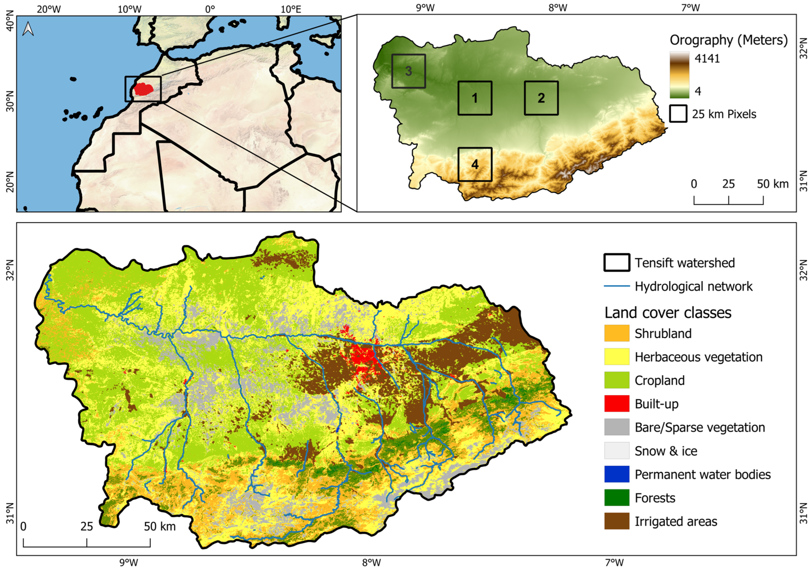
2.1. Study Area

Morocco, as a southern Mediterranean country, has been affected by the impacts of climate change which have caused lower rainfall and higher temperatures [36,37,38]. The Tensift basin (Figure 2) in central Morocco (31°–32°30′N, 7°–10°W, surface of about 22 000 Km²) has an arid to semi-arid Mediterranean climate (Köppen-Geiger Csa). Due to its geographical location, economic and agricultural activity, and population growth, the basin is considered drought prone. The topography is characterized by a plain surrounded by the High Atlas Mountain range at the south and the Jbilet range at the north which serves as sources of water for the surrounding regions. The Haouz plain is crossed by a network of intermittent streams coming from the Atlas.

The plain and Piedmont concentrate most of the agricultural production. The dominant crops are cereals (51% of irrigated areas) and olive trees (30% of irrigated areas), while the non-irrigated part of the plain is cultivated with rainfed wheat [23,39].

In the Tensift region, water resources are mainly used for agriculture, but this proportion has declined from about 92% in the 1990s to around 80% in the 2020s. The irrigated surface areas have increased significantly, and groundwaters are overexploited [23]. In this context, recurrent droughts are having a growing impact on agriculture. The main rule of water resource management is to give absolute priority to drinking water, followed by the preservation of arboriculture [40]. Cereal production is therefore heavily impacted by drought, while arboriculture is more affected by water shortages linked to the semi-arid climate. Morocco, with the Tensift region included, has experienced several periods of drought which have had severe socio-economic repercussions. The Marrakech-Tensift region is one of the Moroccan regions most exposed to agricultural drought. The socio-economic impacts of recent droughts in Morocco, as reported by the Direction de Météorologie Nationale (DMN), have been severe. In 1994–1995, a severe drought led to a 7.6% reduction in GDP in 1995, with cereal production falling from 9.5 million tons in 1994 to just 1.6 million tons in 1995. The following droughts in 1996–1997, 1998–1999, and 1999–2000 further reduced incomes, resulting in GDP declines of 2.3% and 1.5%, respectively, as well as major damage affecting 275,000 people and economic losses amounting to USD 900 million. In 2000–2001, the country had to double its wheat imports, with 5 million tons instead of an average of 2.4 million tons. The drought of 2004–2005 led to a drop in economic growth from 3.5% to 1.3% in 2005. To reduce the impact of extreme drought, the country has embarked on a major national resource mobilization plan, including the construction of 30 large dams, the deployment of desalination stations, and the interconnections between the north and south of the country. The aim is to maintain two years of water consumption to cope with the most severe droughts.

2.2. Dataset

In this study, we used different data derived from several sensors. A summary of the products considered is displayed in

Table 1. Summary of the products considered.

Product	Spatial and Temporal Resolution	Temporal Coverage	Period of Interest	Websites
ERA5Land	9 km/1 M	1950–present	1981–2021	https://cds.climate.copernicus.eu/cdsapp#!/dataset/reanalysis-era5-land-monthly-means?tab=overview, accessed on 5 December 2022
ESA CCI SM	25 km/1 D	1978–2021	2001–2021	https://www.esa-soilmoisture-cci.org/ (last access: 23 October 2022)
MODIS (NDVI)	1 km/1 M	February 2000–near-present	2001–2021	https://lpdaac.usgs.gov/, accessed on 25 March 2021
MODIS (LST)	1 km/1 D	February 2000–near-present	2001–2021	https://lpdaac.usgs.gov/, accessed on 25 March 2021

.

2.2.1. ERA5Land

The ERA5Land reanalysis is derived from ERA5, the fifth generation of the European Centre for Medium-Range Weather Forecasts (ECMWF) reanalysis. It is produced using a 4D-Var scheme, with measurements from various observational systems included in the atmospheric model [41]. Atmospheric meteorological and flux fields from ERA5 are used to force the Tiled ECMWF Scheme for Surface Exchanges over Land (HTESSEL) land surface component (Cy45r1 version) of the Integrated Forecast System (IFS) to generate ERA5Land. Data are available from 1950 to the present day over the entire globe. The grid and temporal resolutions are 9 km and one hour, respectively. For this study, we downloaded monthly average ERA5Land precipitation data for the study period (1981–2021) over the Tensift basin in Morocco.

2.2.2. ESA CCI SM

The European Space Agency’s Climate Change Initiative for Soil Moisture (ESA CCI SM) data were selected because of their long time series (1978–2021). The product comes in three configurations. We used the combined active–passive product version 7.1 (https://esa-soilmoisture-cci.org/, accessed on 23 October 2022). The active soil moisture dataset was produced by merging microwave scatterometers (ERS-1/2 Scatterometer and Metop Advanced Scatterometers). The passive one was generated from multi-channel microwave radiometers (Scanning Multichannel Microwave Radiometer (SMMR), Special Sensor Microwave Imagers (SSM/I), Soil Moisture and Ocean Salinity (SMOS), Advanced Microwave Scanning Radiometer for EOS (AMSR-E), Tropical Rainfall Measuring Mission (TRMM), WindSat, Soil Moisture Active/Passive (TRMM), and the Advanced Microwave Scanning Radiometer 2 (AMSR2)). The product has a daily temporal resolution and spatial sampling of 0.25°. The daily data were aggregated to provide monthly soil moisture values corresponding to the monthly time scale of the satellite data described below.

2.2.3. MODIS Datasets

We used two satellite products from the Moderate Resolution Imaging Spectroradiometer (MODIS), the monthly Normalized Difference Vegetation Index (MOD13A3), and the land surface temperature (LST) (MOD11A1) (https://lpdaac.usgs.gov/, accessed on 25 March 2021). The products have a spatial resolution of 1 km. The daily LST products were aggregated to obtain the monthly time series by calculating the monthly average.

As LST is inherently linked to air temperature (Ta), we also analyzed the difference between Ta and LST. This difference is commonly used in the assessment of evapotranspiration through the energy budget (see for example [42]). Air temperature was retrieved from the 2 m air temperature variable given by ERA5Land and was averaged between two-time steps to air temperature (Ta) at the time of MODIS overpass.

2.3. Methods

2.3.1. Calculation of Drought Indices

For meteorological drought, the calculated index was the SPI (Standardized Precipitation Index) at 1, 3, 6, and 12 months. For agricultural drought, three indices were calculated: the VCI (Vegetation Condition Index), the TCI (Temperature Condition Index), and the SMCI (Soil Moisture Condition Index).

The calculation of the SPI requires a long time series with at least 30 consecutive years of monthly precipitation data to be fitted using a given probability distribution function (log-normal, Gamma, or log-logistic). We opted for the Gamma distribution which has been approved for its relevance in the calculation of the SPI [32,43,44]. The next step was to determine the corresponding frequencies based on the fitted distribution. The frequencies were then converted to the corresponding quantiles of the standard normal distribution [7,45]. The SPI was calculated over the period 1981–2021 to describe temporal variations in meteorological drought using the ERA5Land precipitation component at 9 km resolution and at different time scales (1, 3, 6, and 12 months). The SPI calculation was performed at different time scales depending on the type of drought examined. Negative SPI values indicate dry periods and wet periods are depicted by positive SPI values.

The VCI based on the NDVI, reflects the condition of vegetation during a drought event. It has been used and evaluated in several regions of the world [46,47,48,49]. The VCI is a simple normalization of the NDVI that is intended to present anomalies over a period. The subtraction of 0.5 from the VCI, TCI, and SMCI values was intended to capture negative anomalies in the index time series. In addition, the transformation into a range between −0.5 and 0.5 facilitates the interpretation of anomalies.

The VCI was obtained from the following equation:

$$\mathrm{V}\mathrm{C}\mathrm{I}=\frac{{\mathrm{N}\mathrm{D}\mathrm{V}\mathrm{I}}_{\mathrm{t}}-{\mathrm{N}\mathrm{D}\mathrm{V}\mathrm{I}}_{\mathrm{m}\mathrm{i}\mathrm{n}}}{{\mathrm{N}\mathrm{D}\mathrm{V}\mathrm{I}}_{\mathrm{m}\mathrm{a}\mathrm{x}}-{\mathrm{N}\mathrm{D}\mathrm{V}\mathrm{I}}_{\mathrm{m}\mathrm{i}\mathrm{n}}}-0.5$$

(1)

The maximum and the minimum NDVI were computed for a specific month t, using remotely sensed MODIS-NDVI data from 2001 to 2021.

The TCI was used to determine temperature-related plant stress. The TCI is derived from land surface temperature (LST) and was calculated using MODIS LST (MOD11A1) data. The condition index was scaled from −0.5 to 0.5 for each month over the period of 2001–2021. A second version of the TCI was also computed by replacing LST with the difference between air temperature and surface temperature (Ts − Ta) (TCI2). This difference has the advantage of taking into account the local meteorological conditions. To do so, the air temperature was retrieved from ERA5Land at the time of the MODIS overpass. The monthly version was obtained with the average of (Ts − Ta).

$$\mathrm{T}\mathrm{C}\mathrm{I}=\frac{{\mathrm{L}\mathrm{S}\mathrm{T}}_{\mathrm{m}\mathrm{a}\mathrm{x}}-{\mathrm{L}\mathrm{S}\mathrm{T}}_{\mathrm{t}}}{{\mathrm{L}\mathrm{S}\mathrm{T}}_{\mathrm{m}\mathrm{a}\mathrm{x}}-{\mathrm{L}\mathrm{S}\mathrm{T}}_{\mathrm{m}\mathrm{i}\mathrm{n}}}-0.5$$

(2)

A lack of soil moisture affects crop growth and yields and is therefore widely used to study agricultural drought issues [12]. The SMCI reflects the soil moisture conditions [13].

$$\mathrm{S}\mathrm{M}\mathrm{C}\mathrm{I}=\frac{{\mathrm{S}\mathrm{M}}_{\mathrm{t}}-{\mathrm{S}\mathrm{M}}_{\mathrm{m}\mathrm{i}\mathrm{n}}}{{\mathrm{S}\mathrm{M}}_{\mathrm{m}\mathrm{a}\mathrm{x}}-{\mathrm{S}\mathrm{M}}_{\mathrm{m}\mathrm{i}\mathrm{n}}}-0.5$$

(3)

The indices were calculated spatially, with one spatial datum for the entire basin per month. Then, an average across the basin and selected pixels was calculated was derived to yield a single monthly value. By retaining the original spatial resolutions of the data, the inherent characteristics of each dataset are preserved.

The SPI and SMCI drought indices were calculated over 40 years, while the VCI and TCI indices were calculated over 20 years given the time coverage of the MODIS data used.

2.3.2. Correlation and Cross-Correlation between Indices

The direct relationship between the SPI at different time scales and the VCI, TCI, and SMCI indices were evaluated through use of the Pearson correlation coefficient (R). The used time scales of the SPI are 1, 3, 6, and 12 months, which are specifically associated with agricultural drought conditions. A positive value of R indicates a variation in the variables in the same direction, and if they vary in different directions, the value of R will be negative. It was considered that R between 0.7 and 0.9 indicates a high correlation, between 0.5 and 0.7 indicates a moderate correlation, between 0.3 and 0.5 indicates a low correlation, and less than 0.3 indicates an insignificant correlation.

In addition, a time-lagged correlation analysis (cross-correlation) was performed between the indices at a monthly time scale to define the temporal lag between the agricultural and meteorological droughts. The lagged correlation measures the degree of similarity between a time series and a shifted version of another time series. The correlation peak is at 0 if the time series is synchronized at that moment; if one of the variables leads or delays another, the peak shifts to another time lag where we find the best match between the time series.

A lagged correlation between two drought indices reveals their periodicity and determines the best match in time. The lag time between the SPI and the other indices represents the propagation time of the effect of precipitation deficit on vegetation through its level of development (VCI) and its level of water stress (TCI and SMCI).

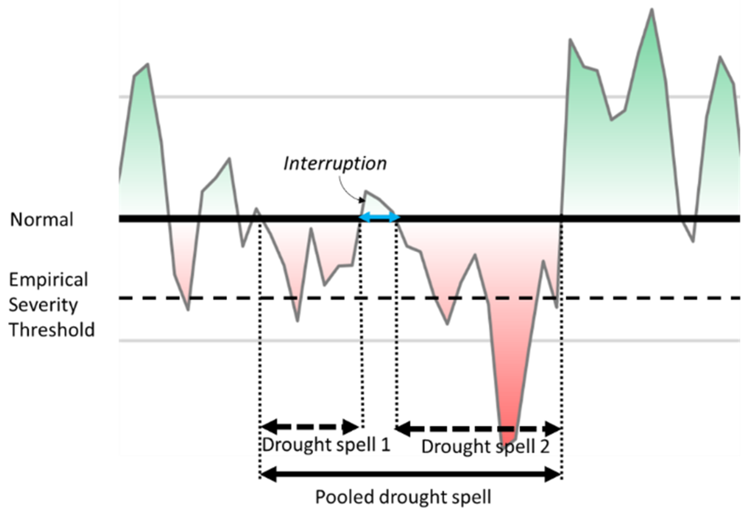
2.3.3. A Modified Run Theory with Pooling and Screening

In this work, we propose to identify drought events according to a parameterized definition [7]. The first parameter corresponds to the onset of a drought event. In the run theory used by [14], this is the value x0. A drought is declared if the index falls below the x0 value. According to [7] when a drought event has been declared, the drought spell starts when it falls below zero and finishes when the index climbs above zero. Instead of using zero, we propose to use a parameter called the normality value, x1. The thresholds x0 and x1 are tested for values of probability of occurrence for the SPI3 and VCI anomaly indices. x0 is tested for values between 5% (usually called the extreme threshold) and 20% (usually called the moderate threshold). The intermediate probabilities are obtained by extracting the probability from the cumulative distribution function. x1 is tested for probabilities between 5% and 50% and is always superior or equal to x0. When x0 = x1, we are in the case of the raw run theory. In the example of Figure 3, it would give two drought events (in red). When x1 = 50%, we are in the case described by [7]. Figure 3a gives a single drought event (dashed area). The two thresholds vary according to the probabilities of occurrence, which is computed with the inverse normal function for the SPI, and which is found empirically for the Tensift region for the other indices (

Table 2. Drought classification based on drought indices and corresponding event probability.

Probability of Occurrence (%)	Drought Category	SPI	VCI	TCI	SMCI
5	Extreme	−1.64	−0.48	−0.49	−0.36
10	Severe	−1.28	−0.4	−0.33	−0.33
15	Moderate	−1.04	−0.36	−0.28	−0.28
20		−0.84	−0.33	−0.24	−0.24
25	Abnormally dry	−0.67	−0.28	−0.2	−0.21
30		−0.52	−0.25	−0.16	−0.18
35	Close to normal	−0.39	−0.23	−0.12	−0.14
40		−0.25	−0.19	−0.09	−0.13
45		−0.13	−0.14	−0.06	−0.09
50		0	−0.1	−0.03	−0.06

). The data were systematically sorted in ascending order based on index values, from minimum to maximum. The counts of occurrences of the index values less than or equal to the current index value were then computed. Subsequently, the probability of occurrence for the current index value was obtained by dividing the count of occurrences by the total number of observations.

An example of the impact of varying x0 and x1 is shown in Figure 3a–c.

We then applied a pooling and screening of drought spells found in the previous step. The pooling technique is generally applied for hydrological drought and for short time scales (daily), but it can also be applied for long-term droughts [20]. We applied the pooling technique described by [21] with an empirical threshold of time $t_c=3$ months (only interruptions shorter than 3 months can be pooled), while the ${\rho }_c$ threshold was computed in the same way but using the magnitude of the drought spell ${\mu }_s$, and the magnitude of the interruption ${\mu }_i$, so that ${\rho }_c=\left|{\mu }_i/{\mu }_s\right|$. The threshold for ${\rho }_c$ was set to 10% according to [20]. To avoid droughts of different categories, only droughts of the same severity can be pooled together. The effect of pooling is shown in Figure 4. The drought spells were finally screened for a short duration. As in [18], the drought spells lasting for less than 3 months were eliminated.

To characterize drought events, a set of descriptors is calculated for each drought event. The first one is the duration which represents the temporal extent of a drought event and is computed as the difference in months between its onset and offset. The second descriptor, magnitude, is obtained by summing the absolute values of the drought index during a drought event. The last is intensity, determined as the ratio between magnitude and duration, and measures the impact of the drought over time.

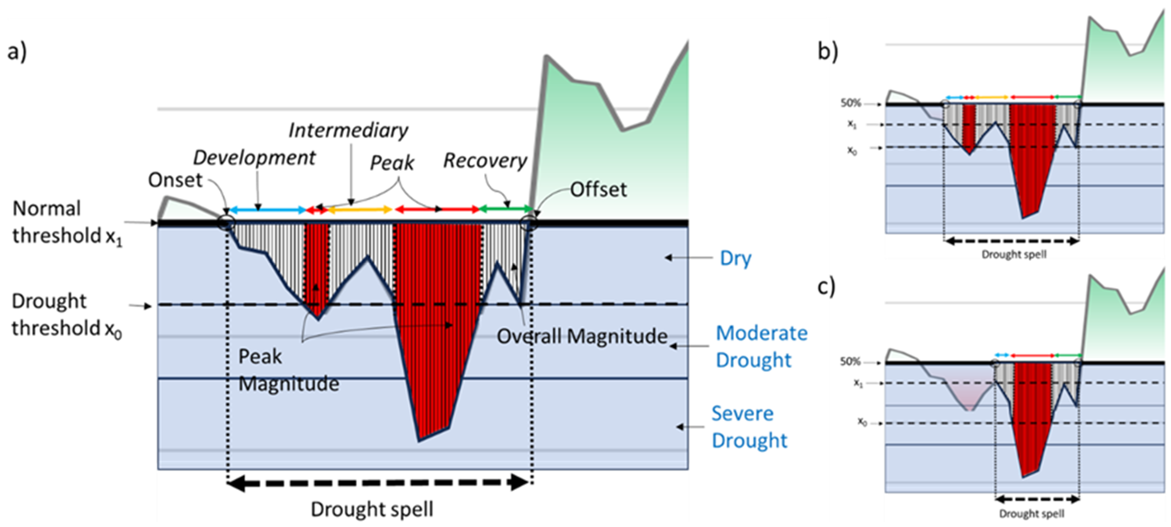
2.3.4. Characterization of Drought Stages Inside a Drought Spell

In order to carry out a more detailed assessment, a drought event is separated into stages, as shown in Figure 3. The ‘development stage’ begins at the onset and ends when the index falls below x0 for the first time. The ‘peak phase’ occurs whenever the indices fall below x0. The ‘recovery phase’ begins when the index climbs above x0 for the last time, and ends at the offset of the drought spell. An ‘Intermediary phase’ may also occur between the peak phases. Finally, ‘Interruption phases’ only occur when drought spells have been pooled.

The various stages of the drought event under consideration will be compared between indices to determine whether or not the stages of a drought event occur simultaneously. A graphic explanation of those phases is given in Figure 3. The interruption phase is shown in Figure 4.

3. Results

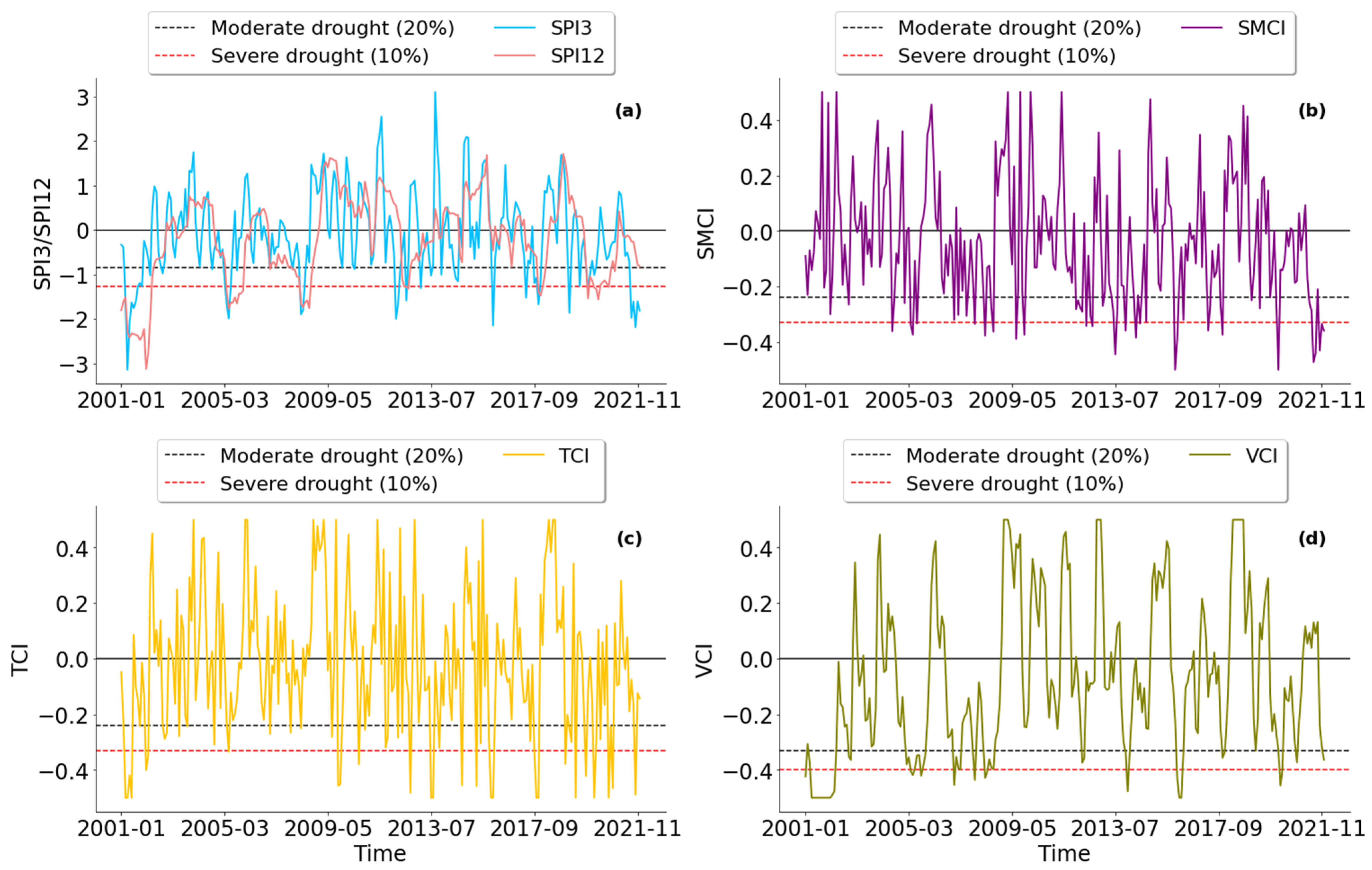
3.1. Time Series of Drought Indices at Different Spatial Scales

The drought events were identified on the time series (2001–2021) of the SPI, SMCI, TCI, and VCI indices using the previously determined thresholds of −0.84, −0.33, −0.24, and −0.24 for moderate drought and −1.28, −0.4, −0.33, −0.33 for severe drought. As depicted in Figure 5, the Tensift basin has gone through multiple periods of drought, with different durations and intensities. The various indices were able to accurately identify dry and rainy periods with a discernible difference between the beginning and end. SPI12 detected eight drought events (Figure 5a), although we excluded summer droughts or those lasting for a month. SPI12 detected the first severe drought since October 2000. After a particularly wet period, the 2004 drought, with less magnitude, lasted for 10 months. The drought returned in January 2007 and persisted until December 2008, with two extremely dry months. The 2017/2018 drought, which began in the summer of 2017 and lasted until April 2018, was moderate but affected the year’s rainy season. A long dry season started in October 2019 followed by two wet months, before the start of another somewhat dry phase.

The agricultural drought indices detected the main droughts identified by the SPI. However, the drought indices differ in the onset, offset, and intensity of dry spells. For example, drought periods identified as moderate by the SPI may be qualified as severe by the other indices. This variation also occurs for wet episodes, where classifications may differ from one index to another. The VCI detected several periods of drought, two of which stood out in terms of duration and magnitude (Figure 5d). The longest period was from October 2006 to November 2008. During this period, drought conditions persisted for an exceptionally long time, with a significant impact on vegetation. The most severe drought was detected in 2001/2002. The SMCI and the TCI fluctuated greatly compared to the other indices, which influences the magnitude and duration of drought periods detected (Figure 5b,c). The most recent drought from January 2019 had the longest duration and severity between 2001 and 2021. The other droughts that were identified matched droughts that the SPI and VCI had previously detected.

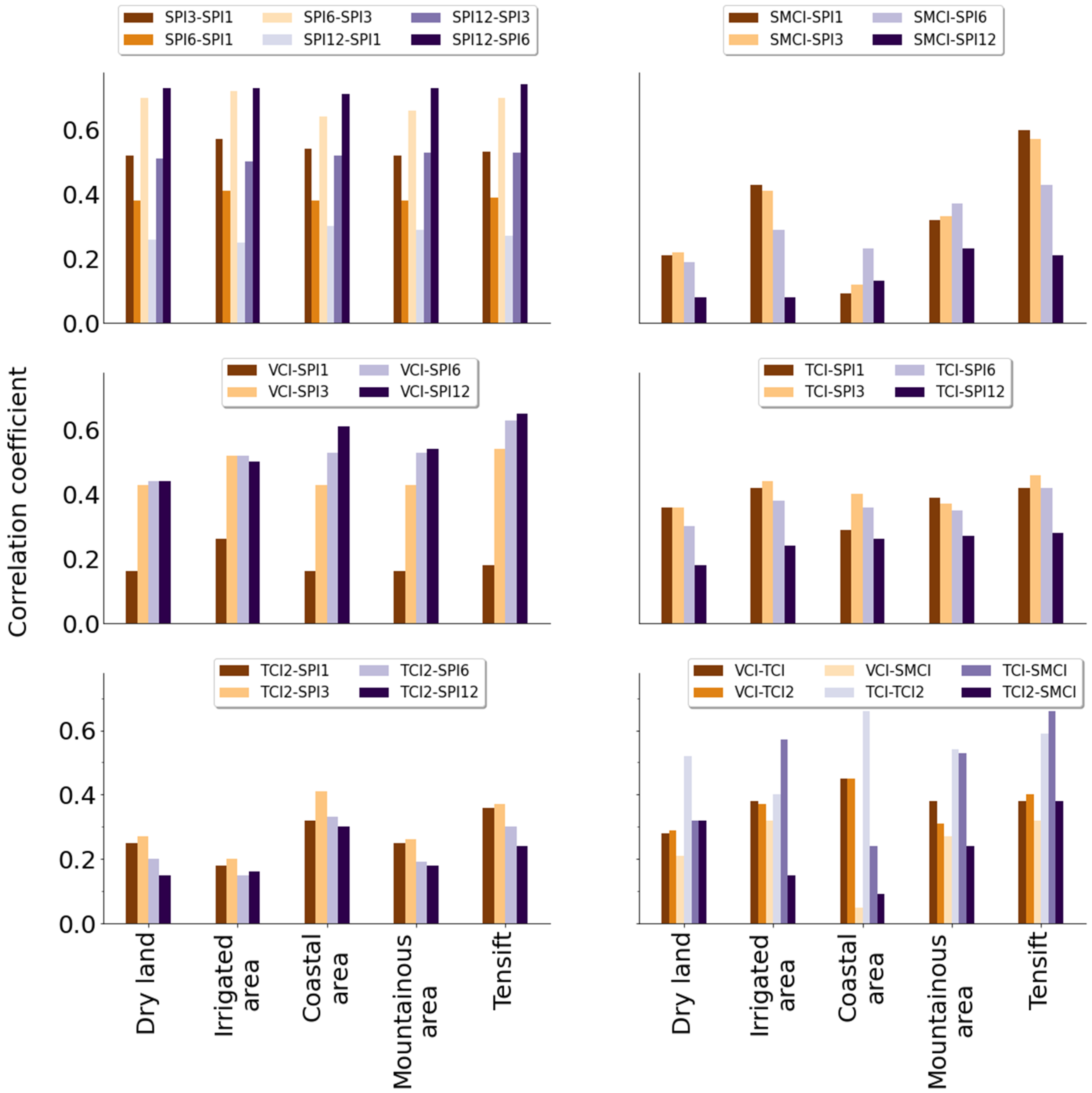
3.2. Pearson Correlation between Drought Indices at Different Spatial Scales

To analyze the direct relationship between droughts, a comparative Pearson correlation analysis was applied to the indices on a monthly time scale, over the whole basin. In addition, the correlation between indices was studied at four pixels of 25 km² inside the basin to assess the eventual effects of spatial variability. The four pixels are 1—”dry land”, a mostly desertic zone with isolated irrigated parcels relying on groundwater, 2—an intensive irrigated zone dominated by perennial tree crops such as olive and orange orchards, 3—a coastal zone mostly covered with natural vegetation close to the outlet of the basin, and 4—a mountainous zone (High Atlas range) with a mix of natural pine forests, bare soil, and some irrigated areas. Those pixels are shown in Figure 2. The multi-scalar correlation analysis is shown in Figure 6.

The correlations in the Tensift basin were high for the SPI pairs. The comparisons between the VCI and the SPI were highest at longer SPI time scales, with a maximum R-value of 0.65 with SPI12. Temperature exhibited a stronger correlation with the monthly and seasonal SPI. A moderate correlation was observed with SPI1 (0.42) and SPI3 (0.46), while on a longer time scale, the correlation coefficient decreased. The same result was obtained with TCI2 but with lower R values. The SMCI was moderately correlated with the seasonal SPI. There was low agreement between the VCI and the SMCI (R = 0.37). The relationship between the VCI, the TCI, and the TCI2 was almost of the same order. Furthermore, the results showed that there was a good relationship between the SMCI and the TCI (0.59).

Concerning the four pixels, the intercomparison of the four SPI scales (1, 3, 6, and 12 months) behaved similarly to the average of the basin, meaning that the SPI does not significantly change over the basin. We then compared the SPI to the satellite indices. For the VCI-SPI pairs, while the mountain and coastal zones behaved similarly to the average basin, the irrigated zone and dry land zone both behaved in the same different manner. R stabilized after 3 months of aggregation (0.5 and 0.44, respectively) when it increased elsewhere (from 0.16 to 0.61 for the coastal area). The fact that the SPI-VCI pair does not increase in those pixels is probably due to irrigation which separates vegetation development from precipitation. Regarding the TCI-SPI pairs, the four pixels behaved in mostly the same way as the basin average, but with lower correlations (from 0.46 in the Tensift basin to 0.36 in the dry land between the TCI and SPI3). A reduction in correlation is tangible for the TCI2-SPI pairs in the irrigated zone (−50%) and also visible in the dryland zone and mountain zone. Irrigation easily explains the decrease in crop water stress explained by this difference in temperature and thus the decrease in correlation as the scale increases. A similar behavior could have been expected with the SMCI-SPI pairs; however, this was not the case. The most important decreases in correlation are seen in the coastal (0.09 between the SMCI and SPI1) and dry land zones (0.08 between the SMCI and SPI12). Also, the irrigated and mountain zones did not behave in the same way as the basin average, which is somewhat abnormal. The behavior of each of the four pixels is very different from the basin average regarding the SMCI–SPI correlations.

The comparison between the agricultural drought indices at the selected pixels showed that each zone shows a very contrasted behavior. The VCI-TCI and VCI-TCI2 were two similar pairs in all cases. However, the correlation between both temperature indices varied from 0.4 (irrigated zone) to 0.6 (coastal zone). Regarding the SMCI, the correlation was almost non-existent with the VCI in the coastal zone and remained insignificant in the dry zone. It was a little more significant in the two other pixels. The correlation of the SMCI with the two temperature indices seemed to corroborate the important loss of correlation in irrigated zones for the TCI2 index. It should also be noted that the correlation in the coastal zone was insignificant. The low to insignificant correlation of the SMCI with the precipitation index in some zones (coastal and dry land) and the low correlations with the temperature indices might also be attributed to the dataset used. For example, it is generally known that the radar signal, whether it be SAR or a scatterometer, cannot reach the soil in specific circumstances, such as those including an important canopy or steep slopes.

Besides this, the Pearson correlations at different scales showed interesting conclusions. As expected, the overall behavior of the basin was a combination of several processes. The SPIs were very homogeneous, which is understandable for a relatively small area such as this basin. The agricultural and meteorological pairs of indices showed contrasted behavior, and the agricultural pairs of indices showed very contrasted behavior from one location to another. The homogeneous correlation of SPIs between the different locations in the basin does not mean that each of them is impacted in the same way by drought. This confirmed that meteorological indices alone are pertinent for regional comparisons but insufficient to explain local behavior. The presence of irrigation, the presence of trees, and the variation in topography were probably the factors that most influenced the differences between these zones.

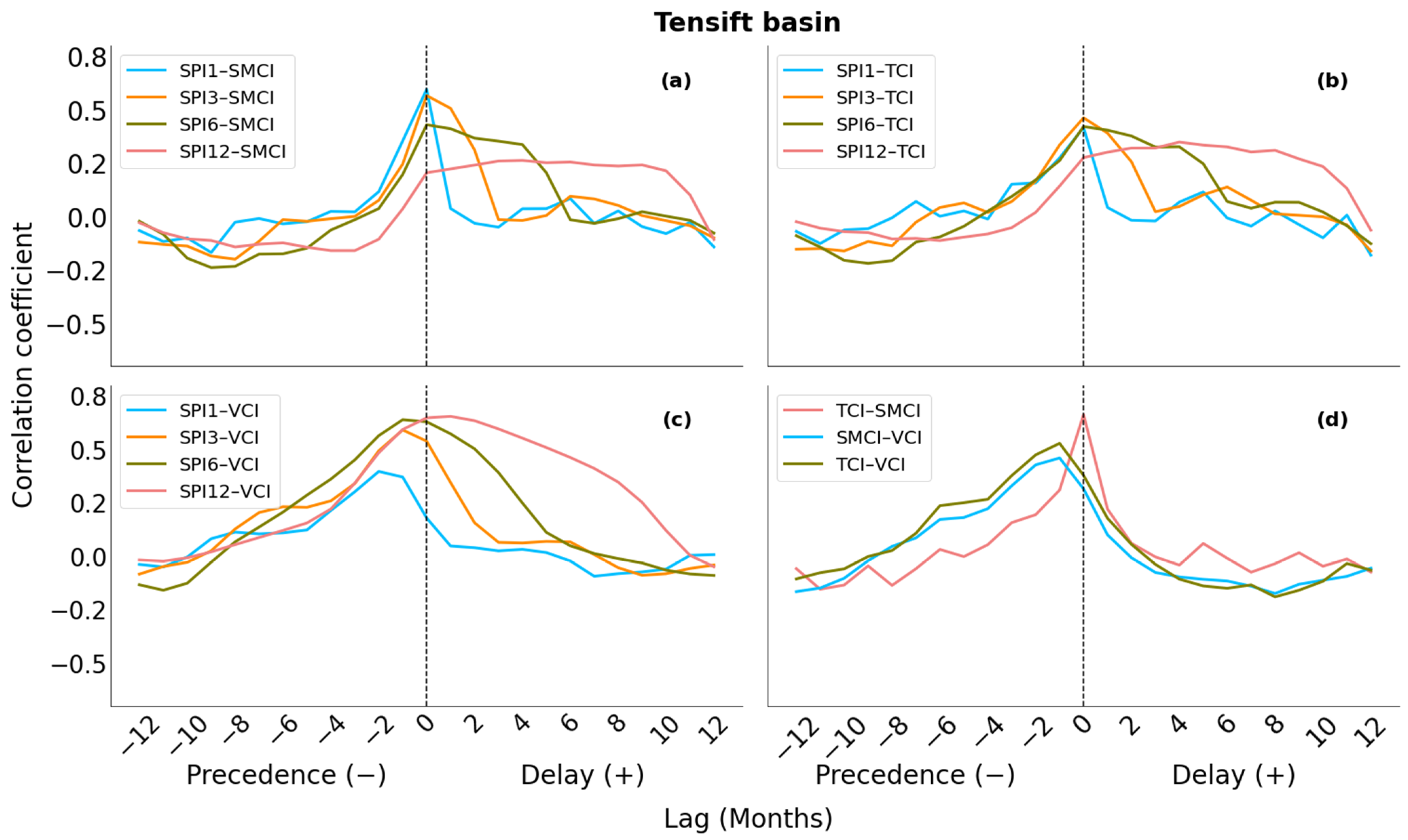
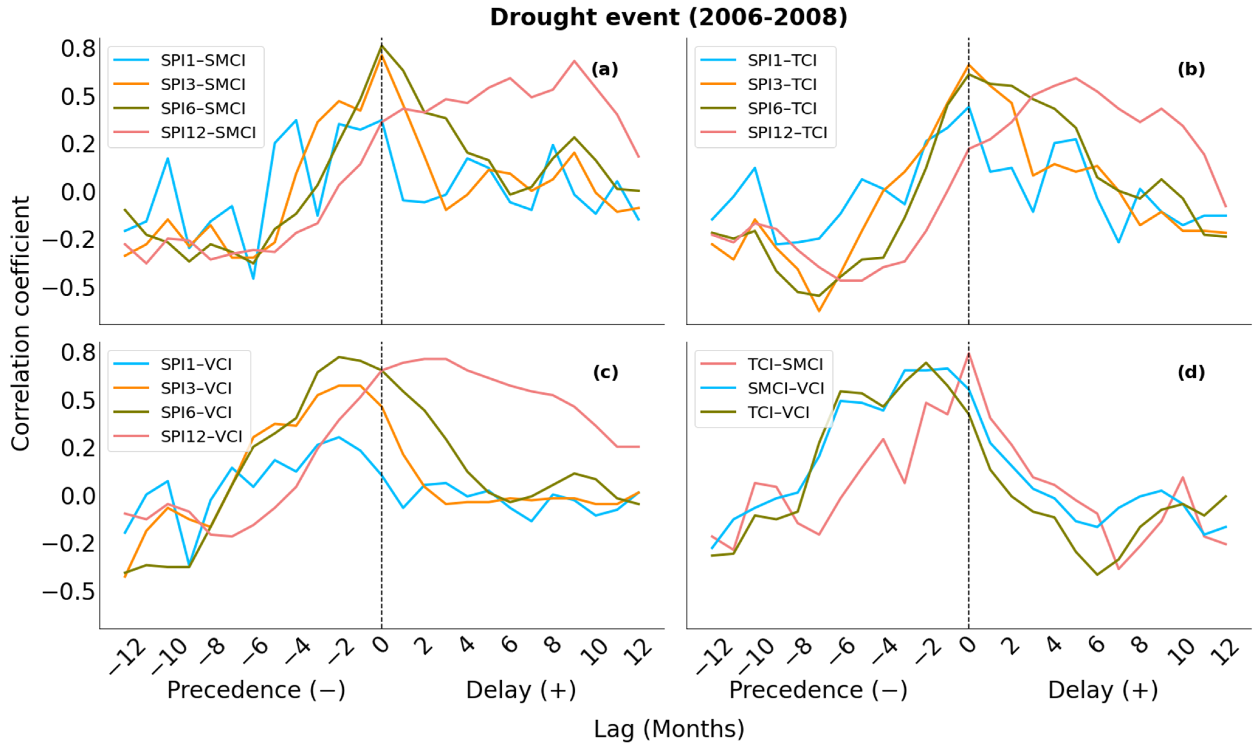
3.3. Cross-Correlation between Drought Indices

The cross-correlation analysis between SPIs (1, 3, 6, and 12 months) and the three agricultural indices (SMCI, TCI, and VCI) was performed to better understand the time delay between the pairs of drought indices. The cross-correlation was implemented with steps of one-month lags ranging from −12 months to +12 months, thus also looking at the symmetry of the cross-correlation. Figure 7 shows the cross-correlation function between the indices time series over the Tensift basin. The second variable is the one that is lagged to the first one. The plots were created using 20 years of monthly data, from 2001 to 2021.

The three first subfigures (Figure 7a–c) show the cross-correlations between the SPIs (1, 3, 6, and 12 months) and the three indices (SMCI, TCI, and VCI). In the SPI approach, the index already incorporates a memory in its conception. The SPI is built to reflect the scalability of drought. It is thus logical that the cross-correlation of the SPI extends in time with the satellite indices. The two indices TCI and SMCI behaved mostly in the same way, with a significant relationship on the right side (positive). The relation fell below significance when the lag came close to the number of months in the SPI (the correlation coefficient fell below 0.2 at 1, 3, 6, and 12 months). On the left side, the relation fell below significance below −1 month. There was no symmetry in the relation. As a result, both the SMCI and the TCI were generally impacted by the SPI’s previous conditions. Over longer SPI aggregation periods, the SMCI, TCI, and SPI correlation values remained positive, indicating the long- and medium-term memory of precipitation on soil moisture and temperature indices.

The results of the comparison between the VCI and the SPI displayed a preceding effect of the VCI with regard to the SPI. It was observed that the leading (negative) range of lags showed higher correlations. SPI-1, SPI-3, and SPI-6 exhibited the same pattern, while peak correlations for these three aggregation periods of SPI were different. The strongest correlations were obtained at −2 months for SPI-1 and −1 month for SPI-3 and SPI-6. Then, with the increasing period of aggregation, this effect tends to propagate towards the positive range of lags. A delay of 1 month was found between SPI12 and the VCI. The same idea previously seen on the TCI and SMCI graphs can be seen again. The one- to two-month lag of the peak on the negative side between the VCI and the SPI reflects the response time of vegetation to precipitation. This means that when precipitation occurs, greenery appears one or two months later. Regarding the two other indices, there is no meaningful lagged response, and the memory of the correlation seems only related to the conception of the SPI.

The last subplot (Figure 7d) shows the lagged relationships between the indices. The best match was found at lag 0, showing good symmetry between the indices in the TCI and SMCI plots. A preceding influence of the SMCI and the TCI on the VCI was observed. The strongest relationships were observed with a temporal lag of −1, showing how soil moisture and temperature regulate vegetation.

The cross-correlation results between the indices for the dry period of 2006–2008 revealed that there were differences in the VCI relationship with the other indices (Figure 8). The delay between vegetation and precipitation was prolonged during the drought period, and the peak, which was at −1 month for SPI3 and SPI6, was observed here at −2 months. Thus, the duration of a precipitation deficit will prolong the vegetation’s response time. In other words, if a precipitation deficit occurs, it will show up in the vegetation after 2 months.

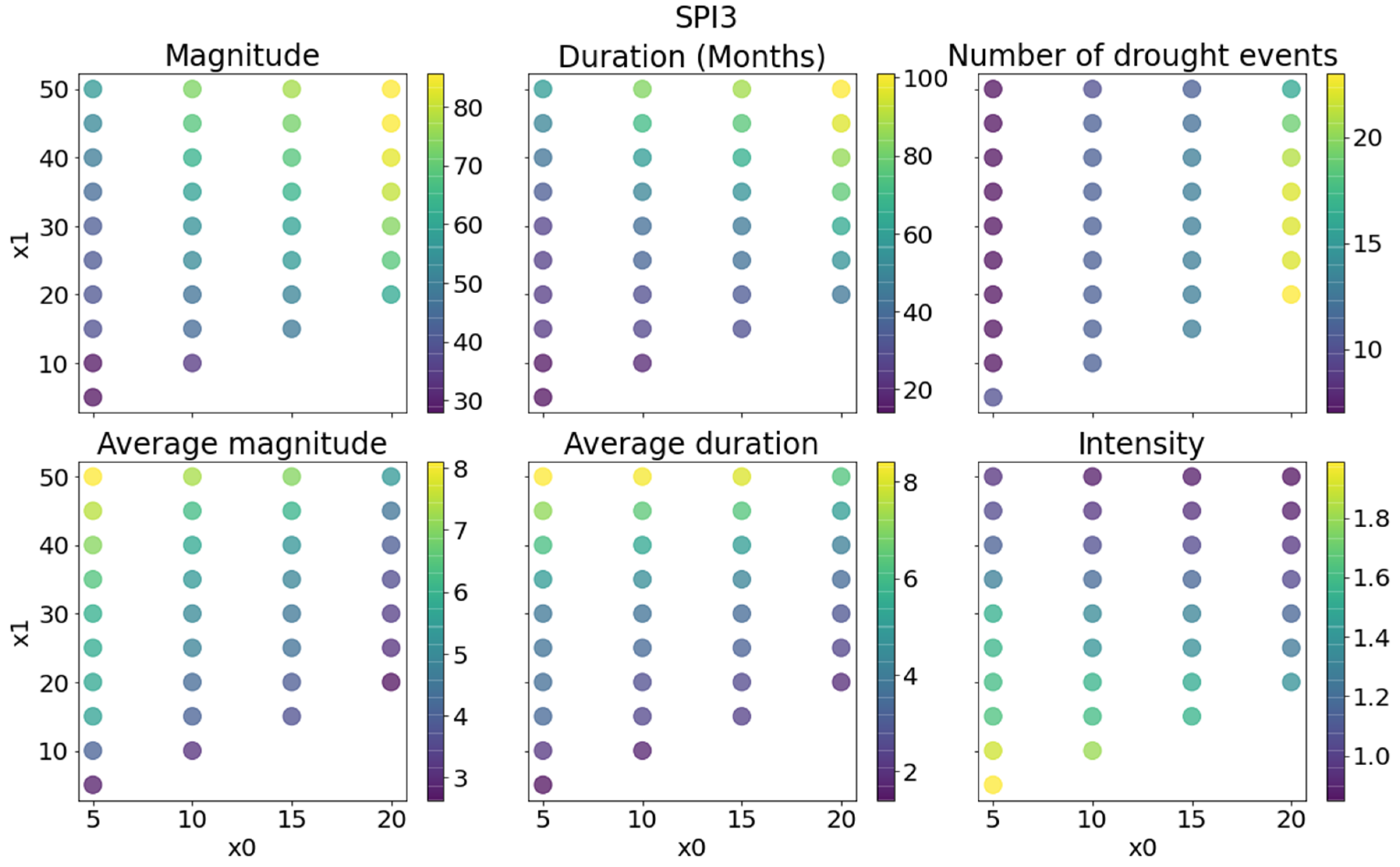
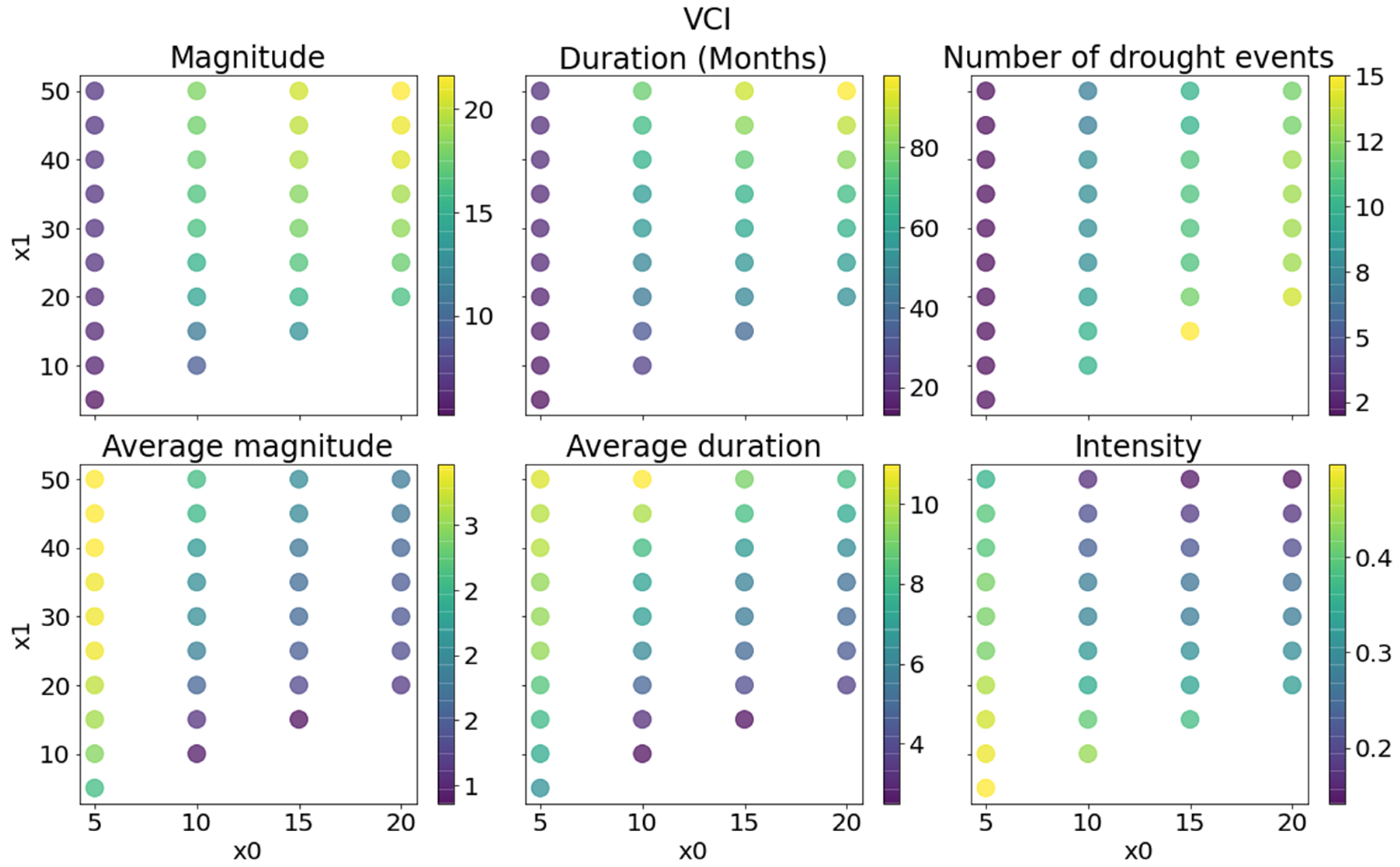
3.4. Run Theory According to a Lower and Upper Bound

Figure 9 and Figure 10 show the results of the drought characteristics extracted for each pair of (x0, x1) to highlight the importance of the choice of these parameters, which directly affect the number of droughts per period and their intensity. The identification of drought events follows a structured process. The initial criterion involves the index falling below the x0 threshold, marking the declaration of a drought. We then go back in time to identify the onset of drought, starting with x1, which serves as the threshold for normal conditions. The drought is terminated when the index rises once again above the x1 threshold. The 25–30% level is generally considered a threshold between dry and drought [26], while the 50% level (which for the SPI means 0) was considered by [7] as the level for normality.

Figure 9 and Figure 10 only show SPI3 and the VCI, since the other indices give roughly similar results. For each pair of thresholds, we obtained the events detected by these thresholds, their magnitude, duration, and intensity, as well as the total number of events. We then calculated the sum of each feature per pair of thresholds. Next, we calculated the average magnitude and duration by dividing the sum calculated above by the number of events detected by each pair of thresholds.

When x0 = x1, this is the run theory with one single threshold. Those are shown on the lower diagonal of Figure 9 and Figure 10. Although, logically, the number of drought events should increase as x0 increases, two consecutive events can overlap. For SPI3, the number of drought events rises from 7 (x0 = 5%) to 23 (x0 = 20%) and increases from 2 to 15 with the VCI. The total duration of the drought periods ranges relatively from 14 months for low x0 to 100 months for high x0. The mean duration is stable and very short for both indices (2 to 11 months). Increasing x0 increased the number of events but not their duration. The total and mean magnitudes follow the same pattern as the duration. Intensity, which is magnitude divided by duration, decreases as x0 increases; this is because the higher the threshold, the more months with a lower magnitude in the drought events dataset.

x1 varies from x0 to 50%. The number of events is not influenced by variations in x1 when x0 is low. The events are too separated and unrelated; however, with higher x0, the number of events significantly decreases when x1 increases (from 23 to 16 for SPI3).

The average duration of events rises logically with increasing x1. For SPI3, it reaches an average of 6 to 8 months for x1 = 50% and 3 months for x1 = 30% (against 2 months when x0 = x1). Magnitude behaves in the same way as duration for both variables. Intensity decreases as x1 increases, meaning that the increase in duration is greater than the increase in magnitude. The increase in average duration due to the use of a second threshold seems more in line with the concept of a slow onset of drought, especially for very low thresholds. The intensity is flattened when increasing x1; however, each event is still well differentiated.

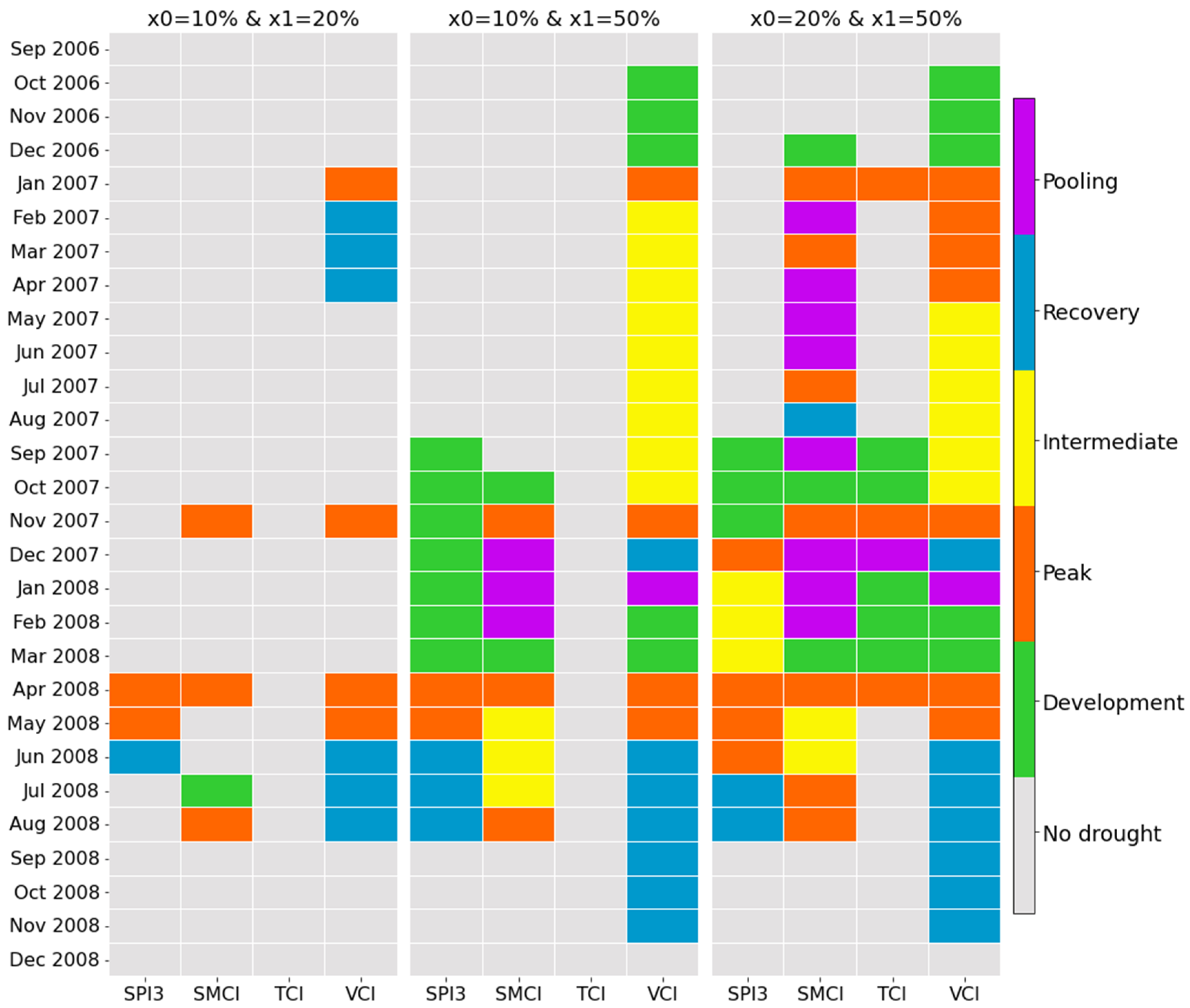
3.5. Drought Stages and Pooling (A Case Study)

The 2006–2008 drought episode is considered as a case study. The episode is divided into several stages. The purpose is to see how the indices behave concerning these stages, and how they vary by changing the normality and drought thresholds. Figure 11 illustrates three scenarios, each defined by unique assignments of values to x0 and x1, namely (10%, 20%), (10%, 50%) and (20%, 50%). Notably, these pairs do not imply the same value at both thresholds x0 and x1.

The results of the three cases studied reveal significant differences in drought detection. With a severe threshold of 10% for x0, the TCI does not detect the drought, whereas it is visible on the other three indices. As the threshold becomes more extreme, the detail of the start and end of the episode takes us directly to its peak without being able to anticipate its onset. By adjusting the normality threshold to 50%, however, we can visualize the different stages of the drought and anticipate its appearance at the start of a development phase. In the third case, where we choose a moderate threshold for x0, several development phases appear, the duration of peaks lengthens and the interconnection between indices becomes more obvious. Interestingly, in this case, the TCI manages to detect the same peaks as the other indices. Furthermore, it appears that the pooling approach is particularly applicable to indices subject to significant fluctuations, such as the SMCI and the VCI. Pooling somehow works like smoothing by connecting periods of drought.

4. Discussion

4.1. Drought Assessment Using Various Indices

Drought assessment using multiple indices enables us to monitor the evolution of drought over time within a specific area, enabling trends in increasing or decreasing drought intensity to be identified. All the indices were able to identify past drought periods, with notable differences in the behavior of each of them. The drought episodes identified using the indices employed in our study are consistent with the findings of previous work. The years 2001, 2004, 2007, 2017, 2019, 2020, and 2021 stand out as the most severe drought periods. These results corroborate the observations of various authors, cited in several works across different regions of Morocco [46,50,51,52], such as the Oum Er-Rbia river basin [53], northwest Morocco [54], the Sebou basin [55], and the Souss basin [56]. These regions, characterized by their semi-arid, arid, and Mediterranean climatic characteristics, have been the focus of previous research, which has also highlighted particularly dry years, in line with our findings. It should be noted that there are discrepancies between the drought seasons identified by various studies in the same regions. These differences can be attributed to the choice of data (in situ or satellite), the specific study period, and the drought indices used. Our results showed remarkable differences between the indices in terms of the characteristics of drought events. The most striking feature is the determination of the onset of drought episodes, which could differ from one index to another. Therefore, given the spatial and temporal complexity of drought, it is difficult and probably inadequate to use a sole index for drought monitoring. The complexity of agricultural drought is linked to various parameters encompassing both climate-related elements (such as insufficient precipitation and extreme heat) and soil-related factors (including soil moisture, water availability in the root zone, and soil types). Consequently, a comprehensive analysis of agricultural drought requires consideration of these diverse variables, which is not fully grasped by a perspective with limited drought indices [57,58,59]. Thus, it was crucial to use a variety of indices to track the beginning and end of drought events.

4.2. Interactions between Drought Indices

The difference between precipitation and actual evapotranspiration (AET) has been used in recent studies [60,61]. However, AET does not fully take into account water demand, and precipitation is not the only source of water, particularly in irrigated areas [62]. The cascade of impact is theoretically better assessed with intermediate variables that can be observed synoptically by remote sensing. At the basin scale, almost all of the examined indices, SPI, VCI, SMCI, TCI, and TCI2, showed a low to moderate correlation, and the best correlations with SPI were recorded with the VCI. This level of correlation between indices has been found in several studies [63,64,65]. When analyzing the correlation between indices at the four agrosystems of the basin, it was underlined that the correlation SPI-SMCI and SPI-VCI dropped in arid and non-irrigated systems. Therefore, the spatial variation within basins could also alter the correlations. This might be related to climatic conditions; the more stressed the humidity conditions are, the weaker the correlations tend to be. The low correlation observed can also be attributed to the method used to calculate the Standardized Precipitation Index (SPI), based on the probability function distribution of precipitation data, which differs from the approach used for other indices. Lastly, the predominance of biophysical processes over the rain–vegetation process is an influential factor that may contribute to these low correlations.

Among the SPI calculation scales, the results showed that the 3-month scale is the one that agreed best with all the indices. Hence, this seasonal scale seems a good compromise for multi-indice drought analyses over long periods. Additionally, amongst the agricultural drought indices, the best correlation at the basin scale was recorded between the TCI and the SMCI; in the context of scarce precipitation, an increase in temperature induces the depletion of soil moisture. However, SMCI and VCI unexpectedly presented a lower correlation. This could be due to the sensitivity of NDVI to soil moisture, which depends on the density of vegetation cover given that wet regions are less sensitive to soil moisture than dry regions with low vegetation density [66].

For the TCI and SMCI indices, the strongest correlations with SPI were found around lag 0. This shows the quick interactions between the indices and SPI. The SPI’s earlier and current conditions affect the SMCI and TCI. All correlations are on the positive side of the graphs, indicating an asymmetrical relationship between the SMCI, TCI, and SPI indices. This asymmetry suggests a significant influence of precipitation on humidity and temperature in our study area. Consequently, there is no significant impact in the opposite direction, reinforcing the unidirectional nature of the influence detected. Another explanation could be the limited soil depth for which the ESA CCI SM product is represented (2–5 cm for the combined product), which restricts its use in such climates because of high temperatures and thus disrupts variations in soil moisture [67].

The VCI showed a preceding influence on the SPI at monthly and seasonal scales, with the peak correlation found in the negative lags for shorter SPIs. It means that vegetation is influenced by the previous moisture conditions and has a response time of two months. The greater the SPI aggregation, the stronger the correlation, on the positive side of the lags. The result is an asymmetrical interaction between the VCI and the SPI. This outcome is coherent with the findings of [30] comparing the evapotranspiration deficit index with the SPI. Those authors interpret this loss of asymmetry as the increase in aggregation. The interactions between the indices revealed the existence of the delay (precedence) response to precipitation deficits. In other words, precipitation deficiencies may be translated into deficits in land surface variables in a delayed manner. The variables’ time response may have significant adverse effects on the basin’s hydrological cycle, resulting in increased water stress, and reduced agricultural productivity.

Temporal resolution has always been a challenge for drought monitoring indices using remotely sensed data. There is not always a clear difference between the length of the aggregation and the time step of the calculation. The most commonly used drought indices are calculated primarily on a monthly basis, with a one-month aggregation. Therefore, interactions between land–soil atmosphere variables are fast-moving in a semi-arid Mediterranean climate. Hence, some studies recommend short time scales for drought assessment [30]. Multi-monthly aggregation has already been tackled with the multi-scalar approach of the SPI; nevertheless, smaller aggregations are generally not considered, because the SPI becomes very noisy. The aggregation time of indices such as the NDVI, LST, and SM is not straightforward and could be further investigated. Also, when indices are aggregated beyond the seasonal scale, interaction analysis may be ambiguous due to the high influence of aggregation when using a long-time scale.

The time response of the agricultural drought to precipitation deficits can be influenced by several factors. Namely, the initial conditions of water resources in the basin play an important role in the occurrence or recovery of the drought [68]. This raises uncertainties about the transmission of precipitation deficits to the vegetation (non-linear) [17,68,69]. This is due to the properties of the watersheds which can induce different propagation processes, and which are controlled by the elevation which is connected to snow processes and land covers. The latter influences the propagation of drought through the modification of evapotranspiration and the distribution of precipitation between evapotranspiration and streamflow [17,70]. Additionally, irrigation remains a problem in quantifying the response time of vegetation to precipitation deficits. This anthropogenic factor affects the interactions by altering the duration and intensity of the drought (e.g., if a drought occurs and irrigation persists, it will further hasten the drought process) [71].

4.3. Drought Characteristics and Stages

The drought events post-processing with the identification of stages, the possibility of pooling minor events, and also the possibility (not displayed here) of screening short events are appealing. Analysis of a single index allows us to distinguish between stages. In particular, the slow onsets and offsets mentioned by the WMO are found in the development and recovery stages. In the development stage, we are not really into drought, but the diagnostic knows that there is a peak coming after, so this is part of the drought event. The same can be said about the recovery. Intermediate stages are also interesting, especially for remote sensing observations. For example, the vegetation index not recovering back to “normality” between two peaks probably means that the vegetation had been lastingly affected by drought. The pooling that was previously used essentially for hydrological drought also appeared to be an interesting tool for connecting both slow-moving indices (the VCI) and fast-moving indices (the SMCI and the TCI).

Finally, if the cascade of impact is not always evident with the selected indices, it has been shown that a longer delay can be seen in vegetation. In contrast, the two other indices are more erratic and immediate. Simple combinations of indices have been formulated in various studies. [72] simply averaged vegetation and brightness temperature. [19] summed three indices: at least two out of three indices below the moderate threshold mean drought. [29] considered that there is a precedence between indices to propose an emergency index. With the objective of forecasting cereal yield, [1] used a non-linear combination of indices obtained from remote sensing. Also, the Global Drought Index (GDI) proposed by [62] weighs how the proportion of soil or vegetation is important for the drought index; thus, the GDI takes into account the seasonality of vegetation. All of these different approaches, the two thresholds run theory technique detailed here, and the separation in phases provide interesting hints for combining multiple indices.

4.4. Improving Drought Preparedness through the Timely Representation of Drought Onset

Timely representation of the onset of drought can contribute to the adoption of proactive measures, which lies in the more effective management of water supply and demand. First, it is imperative to control water demand, particularly in the urban, industrial, and agricultural sectors. With a significant increase in urban and industrial demand, more rigorous management is needed. In particular, agricultural demand accounts for a preponderant contribution (~80%) and is currently poorly regulated. On the other hand, it is essential to offer a resilient water supply in the face of prolonged drought events. This implies the increased mobilization of water resources and their storage to meet needs during crises. In addition, the preservation of groundwater as a natural stock is crucial to ensuring a sustainable supply of water adapted to changing climatic conditions.

5. Conclusions

In the present study, we used remote sensing data to construct drought indices and understand interactions between meteorological and agricultural droughts in a Mediterranean semi-arid basin.

Four drought indices were calculated. The meteorological index SPI was determined from ERA5Land data at different time scales of 1, 3, 6, and 12 months. The agricultural drought indices VCI (Vegetation Condition Index, from MODIS-NDVI), TCI (Temperature Condition Index, from MODIS LST and ERA5Land data), and SMCI (Soil Moisture Condition Index, from ESA CCI SM) were calculated at a monthly time scale. Satellite drought indices have already proven to be a useful tool for monitoring drought and its impacts on agriculture.

The results of the Pearson correlations revealed the effect of the spatial variability of the different agrosystems on the drought indices’ concordances. The behavior of the basin as a whole is a fusion of several heterogeneous entities. The interpretation of spatially aggregated drought indices should be carried out with care, and the aggregation should probably be applied to homogeneous areas. Homogeneously connected SPIs do not reveal the impact of drought on different regions, in contrast with the divergent behavior of the agricultural drought indices. Thus, meteorological indices are significant for regional comparisons but are insufficient to explain local patterns.

Additionally, the results proved rapid responses of temperature and soil moisture to precipitation deficits in a semi-arid Mediterranean climate. The VCI is influenced by the previous moisture conditions, especially in dry conditions. The SMCI and the TCI showed an instantaneous response to the SPI. The correlation between the SMCI, the TCI, and the SPI remains significant, suggesting long- and medium-term precipitation memory.

We have proposed to modify the run theory by introducing a normality threshold. The agricultural drought indices were able to detect the drought periods that the SPI pointed out. Every index may accurately identify drought periods with a contrast between the beginning and ends and in some cases a contrast in the intensities of the drought. Several changes affect the characteristics of drought by modifying the thresholds of normality and dryness (x0 and x1, respectively). The arbitrary choice of the two thresholds can lead to biased information on the duration, intensity, and frequency of droughts. Objective thresholds need to be established to distinguish drought periods, avoid inconsistent conclusions, and improve the comparability of research carried out in the same areas. Furthermore, drought episodes can be connected, but it is crucial to use a variety of indices to assess agricultural drought.

References

1. Bouras, E.H.; Jarlan, L.; Er-Raki, S.; Balaghi, R.; Amazirh, A.; Richard, B.; Khabba, S. Cereal yield forecasting with satellite drought-based indices, weather data and regional climate indices using machine learning in Morocco. Remote Sens. 2021, 13, 3101. [Google Scholar] [CrossRef]
2. Javed, T.; Zhang, J.; Bhattarai, N.; Sha, Z.; Rashid, S.; Yun, B.; Ahmad, S.; Henchiri, M.; Kamran, M. Drought characterization across agricultural regions of China using standardized precipitation and vegetation water supply indices. J. Clean. Prod. 2021, 313, 127866. [Google Scholar] [CrossRef]
3. Klos, R.J.; Wang, G.G.; Bauerle, W.L.; Rieck, J.R. Drought impact on forest growth and mortality in the southeast.pdf. Ecol. Appl. 2009, 19, 699–708. [Google Scholar] [CrossRef] [PubMed]
4. Zscheischler, J.; Martius, O.; Westra, S.; Bevacqua, E.; Raymond, C.; Horton, R.M.; van den Hurk, B.; AghaKouchak, A.; Jézéquel, A.; Mahecha, M.D.; et al. A typology of compound weather and climate events. Nat. Rev. Earth Environ. 2020, 1, 333–347. [Google Scholar] [CrossRef]
5. De Rosnay, J. Le macroscope. Vers une vision globale. Rev. D’histoire Et De Philos. Relig. 1975, 57, 314. [Google Scholar]
6. Heim, R.R., Jr. A review of twentieth-century drought indices used in the United States. Bull. Am. Meteorol. Soc. 2002, 83, 1149–1166. [Google Scholar] [CrossRef]
7. McKee, T.B.; Nolan, J.; Kleist, J. The relationship of drought frequency and duration to time scales. Prepr. Eighth Conf. Appl. Climatol. Am. Meteor Soc. 1993, 17, 179–184. [Google Scholar]
8. Beguería, S.; Vicente-Serrano, S.M.; Reig, F.; Latorre, B. Standardized precipitation evapotranspiration index (SPEI) revisited: Parameter fitting, evapotranspiration models, tools, datasets and drought monitoring. Int. J. Climatol. 2014, 34, 3001–3023. [Google Scholar] [CrossRef]
9. Vicente-Serrano, S.M.; Beguería, S.; López-Moreno, J.I. A multiscalar drought index sensitive to global warming: The standardized precipitation evapotranspiration index. J. Clim. 2010, 23, 1696–1718. [Google Scholar] [CrossRef]
10. Peters, A.J.; Walter-Shea, E.A.; Ji, L.; Vina, A.; Hayes, M.; Svoboda, M.D. Drought monitoring with NDVI-based Standardized Vegetation Index. Photogramm. Eng. Remote Sens. 2002, 68, 71–75. [Google Scholar]
11. Kogan, F.N. Remote sensing of weather impacts on vegetation in non-homogeneous areas. Int. J. Remote Sens. 1990, 11, 1405–1419. [Google Scholar] [CrossRef]
12. Tramblay, Y.; Seguí, P.Q. Estimating soil moisture conditions for drought monitoring with random forests and a simple soil moisture accounting scheme. Nat. Hazards Earth Syst. Sci. 2022, 1, 1325–1334. [Google Scholar] [CrossRef]
13. Zhang, A.; Jia, G. Monitoring meteorological drought in semiarid regions using multi-sensor microwave remote sensing data. Remote Sens. Environ. 2013, 134, 12–23. [Google Scholar] [CrossRef]
14. Yevjevich, V. An objective approach to definitions and investigations of continental hydrologic droughts. J. Hydrol. 1967, 7, 353. [Google Scholar] [CrossRef]
15. Raposo, V.d.M.B.; Costa, V.A.F.; Rodrigues, A.F. A review of recent developments on drought characterization, propagation, and influential factors. Sci. Total Environ. 2023, 898, 165550. [Google Scholar] [CrossRef]
16. Van Loon, A.F. Hydrological drought explained. Wiley Interdiscip. Rev. Water 2015, 2, 359–392. [Google Scholar] [CrossRef]
17. Zhang, X.; Hao, Z.; Singh, V.P.; Zhang, Y.; Feng, S.; Xu, Y.; Hao, F. Drought propagation under global warming: Characteristics, approaches, processes, and controlling factors. Sci. Total Environ. 2022, 838, 156021. [Google Scholar] [CrossRef]
18. Mo, K.C. Drought onset and recovery over the United States. J. Geophys. Res. Atmos. 2011, 116, D20. [Google Scholar] [CrossRef]
19. Spinoni, J.; Vogt, J.V.; Naumann, G.; Barbosa, P.; Dosio, A. Will drought events become more frequent and severe in Europe. Int. J. Climatol. 2018, 38, 1718–1736. [Google Scholar] [CrossRef]
20. Tallaksen, L.M.; Madsen, H.; Clausen, B. On the definition and modelling of streamflow drought duration and deficit volume. Hydrol. Sci. J. 1997, 42, 15–33. [Google Scholar] [CrossRef]
21. Tu, X.; Singh, V.P.; Chen, X.; Ma, M.; Zhang, Q.; Zhao, Y. Uncertainty and variability in bivariate modeling of hydrological droughts. Stoch. Environ. Res. Risk Assess. 2016, 30, 1317–1334. [Google Scholar] [CrossRef]
22. Spinoni, J.; Barbosa, P.; Bucchignani, E.; Cassano, J.; Cavazos, T.; Christensen, J.H.; Christensen, O.B.; Coppola, E.; Evans, J.; Geyer, B.; et al. Future Global Meteorological Drought Hot Spots: A Study Based on CORDEX Data. J. Clim. 2020, 33, 3635–3661. [Google Scholar] [CrossRef]
23. Le Page, M.; Fakir, Y.; Jarlan, L.; Boone, A.; Berjamy, B.; Khabba, S.; Zribi, M. Projection of irrigation water demand based on the simulation of synthetic crop coefficients and climate change. Hydrol. Earth Syst. Sci. 2021, 25, 637–651. [Google Scholar] [CrossRef]
24. Dracup, J.A.; Lee, K.S.; Paulson, E.G. On the statistical characteristics of drought events. Water Resour. Res. 1980, 16, 289–296. [Google Scholar] [CrossRef]
25. Vidal, J.-P.; Martin, E.; Franchistéguy, L.; Habets, F.; Soubeyroux, J.-M.; Blanchard, M.; Baillon, M. Multilevel and multiscale drought reanalysis over France with the Safran-Isba-Modcou hydrometeorological suite. Hydrol. Earth Syst. Sci. 2010, 14, 459–478. [Google Scholar] [CrossRef]
26. Svoboda, M.; LeComte, D.; Hayes, M.; Heim, R.; Gleason, K.; Angel, J.; Rippey, B.; Tinker, R.; Palecki, M.; Stooksbury, D.; et al. The drought monitor. Bull. Am. Meteorol. Soc. 2002, 83, 1181–1190. [Google Scholar] [CrossRef]
27. Bonsal, B.R.; Wheaton, E.E.; Meinert, A.; Siemens, E. Characterizing the Surface Features of the 1999–2005 Canadian Prairie Drought in Relation to Previous Severe Twentieth Century Events. Atmosphere-Ocean 2011, 49, 320–338. [Google Scholar] [CrossRef]
28. Parry, S.; Prudhomme, C.; Wilby, R.L.; Wood, P.J. Drought termination: Concept and characterization. Prog. Phys. Geogr. Earth Environ. 2016, 40, 743–767. [Google Scholar] [CrossRef]
29. Sepulcre-Canto, G.; Horion, S.; Singleton, A.; Carrao, H.; Vogt, J. Development of a Combined Drought Indicator to detect agricultural drought in Europe. Nat. Hazards Earth Syst. Sci. 2012, 12, 3519–3531. [Google Scholar] [CrossRef]
30. Gaona, J.; Quintana-Segui, P.; Escorihuela, J.M.; Boone, A.; Llasat, M.C. Interactions between precipitation, evapotranspiration and soil moisture-based indices to characterize drought with high-resolution remote sensing and land-surface model data. Nat. Hazards Earth Syst. Sci. Discuss. 2022, 22, 3461–3485. [Google Scholar] [CrossRef]
31. Jain, V.K.; Pandey, R.P.; Jain, M.K.; Byun, H.-R. Comparison of drought indices for appraisal of drought characteristics in the Ken River Basin. Weather. Clim. Extrem. 2015, 8, 1–11. [Google Scholar] [CrossRef]
32. Liu, Q.; Zhang, S.; Zhang, H.; Bai, Y.; Zhang, J. Monitoring drought using composite drought indices based on remote sensing. Sci. Total Environ. 2020, 711, 134585. [Google Scholar] [CrossRef]
33. Pei, Z.; Fang, S.; Wang, L.; Yang, W. Comparative analysis of drought indicated by the SPI and SPEI at various timescales in inner Mongolia, China. Water 2020, 12, 1925. [Google Scholar] [CrossRef]
34. Silva, T.; Pires, V.; Cota, T.; Silva, Á. Detection of Drought Events in Setúbal District: Comparison between Drought Indices. Atmosphere 2022, 13, 536. [Google Scholar] [CrossRef]
35. Vergni, L.; Todisco, F.; Di Lena, B. Evaluation of the similarity between drought indices by correlation analysis and Cohen’s Kappa test in a Mediterranean area. Nat. Hazards 2021, 108, 2187–2209. [Google Scholar] [CrossRef]
36. El Moçayd, N.; Kang, S.; Eltahir, E.A.B. Climate change impacts on the Water Highway project in Morocco. Hydrol. Earth Syst. Sci. 2020, 24, 1467–1483. [Google Scholar] [CrossRef]
37. Tramblay, Y.; Badi, W.; Driouech, F.; El Adlouni, S.; Neppel, L.; Servat, E. Climate change impacts on extreme precipitation in Morocco. Glob. Planet. Change 2012, 82–83, 104–114. [Google Scholar] [CrossRef]
38. Tramblay, Y.; Jarlan, L.; Hanich, L.; Somot, S. Future Scenarios of Surface Water Resources Availability in North African Dams. Water Resour. Manag. 2018, 32, 1291–1306. [Google Scholar] [CrossRef]
39. Kharrou, M.H.; Simonneaux, V.; Er-Raki, S.; Le Page, M.; Khabba, S.; Chehbouni, A. Assessing irrigation water use with remote sensing-based soil water balance at an irrigation scheme level in a semi-arid region of Morocco. Remote Sens. 2021, 13, 1133. [Google Scholar] [CrossRef]
40. Le Page, M.; Berjamy, B.; Fakir, Y.; Bourgin, F.; Jarlan, L.; Abourida, A.; Benrhanem, M.; Jacob, G.; Huber, M.; Sghrer, F.; et al. An Integrated DSS for Groundwater Management Based on Remote Sensing. The Case of a Semi-arid Aquifer in Morocco. Water Resour. Manag. 2012, 26, 3209–3230. [Google Scholar] [CrossRef]
41. Hersbach, H.; Bell, B.; Berrisford, P.; Hirahara, S.; Horányi, A.; Muñoz-Sabater, J.; Nicolas, J.; Peubey, C.; Radu, R.; Schepers, D.; et al. The ERA5 global reanalysis. Q. J. R. Meteorol. Soc. 2020, 146, 1999–2049. [Google Scholar] [CrossRef]
42. Senay, G.B.; Schauer, M.; Friedrichs, M.; Velpuri, N.M.; Singh, R.K. Satellite-based water use dynamics using historical Landsat data (1984–2014) in the southwestern United States. Remote Sens. Environ. 2017, 202, 98–112. [Google Scholar] [CrossRef]
43. Livada, I.; Assimakopoulos, V.D. Spatial and temporal analysis of drought in Greece using the Standardized Precipitation Index (SPI). Theor. Appl. Climatol. 2007, 89, 143–153. [Google Scholar] [CrossRef]
44. Sobral, B.S.; de Oliveira-Júnior, J.F.; de Gois, G.; Pereira-Júnior, E.R.; Terassi, P.M.d.B.; Muniz-Júnior, J.G.R.; Lyra, G.B.; Zeri, M. Drought characterization for the state of Rio de Janeiro based on the annual SPI index: Trends, statistical tests and its relation with ENSO. Atmos. Res. 2019, 220, 141–154. [Google Scholar] [CrossRef]
45. Bai, X.; Wang, P.; He, Y.; Zhang, Z.; Wu, X. Assessing the accuracy and drought utility of long-term satellite-based precipitation estimation products using the triple collocation approach. J. Hydrol. 2021, 603, 127098. [Google Scholar] [CrossRef]
46. Bouras, E.H.; Jarlan, L.; Er-Raki, S.; Albergel, C.; Richard, B.; Balaghi, R.; Khabba, S. Linkages between rainfed cereal production and agricultural drought through remote sensing indices and a land data assimilation system: A case study in Morocco. Remote Sens. 2020, 12, 4018. [Google Scholar] [CrossRef]
47. Jiménez-Donaire, M.d.P.; Tarquis, A.; Giráldez, J.V. Evaluation of a combined drought indicator and its potential for agricultural drought prediction in southern Spain. Nat. Hazards Earth Syst. Sci. 2020, 20, 21–33. [Google Scholar] [CrossRef]
48. Jiao, W.; Tian, C.; Chang, Q.; Novick, K.A.; Wang, L. A new multi-sensor integrated index for drought monitoring. Agric. For. Meteorol. 2019, 268, 74–85. [Google Scholar] [CrossRef]
49. Quiring, S.M.; Ganesh, S. Evaluating the utility of the Vegetation Condition Index (VCI) for monitoring meteorological drought in Texas. Agric. For. Meteorol. 2010, 150, 330–339. [Google Scholar] [CrossRef]
50. Ezzine, H.; Bouziane, A.; Ouazar, D. Seasonal comparisons of meteorological and agricultural droughtindices in Morocco using open short time-series data. Int. J. Appl. Earth Obs. Geoinf. 2014, 26, 36–48. [Google Scholar] [CrossRef]
51. Layati, E.; Ouigmane, A.; Qadem, A.; El Ghachi, M. Characterization and Quantification of Meteorological Drought in the Oued El-Abid Watershed, Central High Atlas, Morocco (1980–2019). Hydrospatial Anal. 2021, 5, 45–55. [Google Scholar] [CrossRef]
52. Zkhiri, W.; Tramblay, Y.; Hanich, L.; Jarlan, L.; Ruelland, D. Spatiotemporal characterization of current and future droughts in the High Atlas basins (Morocco). Theor. Appl. Climatol. 2019, 135, 593–605. [Google Scholar] [CrossRef]
53. Zhim, S.; Larabi, A.; Brirhet, H. Analysis of precipitation time series and regional drought assessment based on the standardized precipitation index in the Oum Er-Rbia basin (Morocco). Arab. J. Geosci. 2019, 12, 1998–2000. [Google Scholar] [CrossRef]
54. Acharki, S.; Singh, S.K.; Couto, E.V.D.; Arjdal, Y.; Elbeltagi, A. Spatio-temporal distribution and prediction of agricultural and meteorological drought in a Mediterranean coastal watershed via GIS and machine learning. Phys. Chem. Earth 2023, 131, 103425. [Google Scholar] [CrossRef]
55. Hakam, O.; Baali, A.; EL Kamel, T.; Youssra, A.; Azennoud, K. Comparative evaluation of various drought indices (DIs) to monitor drought status: A case study of Moroccan Lower Sebou basin. Kuwait J. Sci. 2022, 49, 1–25. [Google Scholar] [CrossRef]
56. Ait Brahim, Y.; Seif-Ennasr, M.; Malki, M.; N’da, B.; Choukrallah, R.; El Morjani, Z.E.A.; Sifeddine, A.; Abahous, H.; Bouchaou, L. Assessment of climate and land use changes: Impacts on groundwater resources in the Souss-Massa river basin. Handb. Environ. Chem. 2017, 53, 121–142. [Google Scholar] [CrossRef]
57. Dalezios, N.R.; Gobin, A.; Tarquis Alfonso, A.M.; Eslamian, S. Agricultural Drought Indices: Combining Crop, Climate, and Soil Factors. In Handbook of Drought and Water Scarcity, Principles of Drought and Water Scarcity; Eslamian, S., Eslamian, F., Eds.; CRC Press: New York, NY, USA, 2017; Volume 1, pp. 73–90. [Google Scholar] [CrossRef]
58. Sánchez, N.; González-Zamora, Á.; Piles, M.; Martínez-Fernández, J.A. New Soil Moisture Agricultural Drought Index (SMADI) Integrating MODIS and SMOS Products: A Case of Study over the Iberian Peninsula. Remote Sens. 2016, 8, 287. [Google Scholar] [CrossRef]
59. Xu, Y.; Wang, L.; Ross, K.W.; Liu, C.; Berry, K. Standardized soil moisture index for drought monitoring based on soil moisture active passive observations and 36 years of North American Land Data Assimilation System data: A case study in the Southeast United States. Remote Sens. 2018, 10, 301. [Google Scholar] [CrossRef]
60. Farhani, N.; Carreau, J.; Kassouk, Z.; Le Page, M.; Chabaane, Z.L.; Boulet, G. Analysis of Multispectral Drought Indices in Central Tunisia. Remote Sens. 2022, 14, 1813. [Google Scholar] [CrossRef]
61. Vicente-Serrano, S.M.; Miralles, D.G.; Domínguez-Castro, F.; Azorin-Molina, C.; El Kenawy, A.; McVicar, T.R.; Tomás-Burguera, M.; Beguería, S.; Maneta, M.; Peña-Gallardo, M. Global assessment of the standardized evapotranspiration deficit index (SEDI) for drought analysis and monitoring. J. Clim. 2018, 31, 5371–5393. [Google Scholar] [CrossRef]
62. Zribi, M.; Nativel, S.; Le Page, M. Analysis of Agronomic Drought in a Highly Anthropogenic Context Based on Satellite Monitoring of Vegetation and Soil Moisture. Remote Sens. 2021, 13, 2698. [Google Scholar] [CrossRef]
63. Ji, L.; Peters, A.J. Assessing vegetation response to drought in the northern Great Plains using vegetation and drought indices. Remote Sens. Environ. 2003, 87, 85–98. [Google Scholar] [CrossRef]
64. Vicente-Serrano, S.M.; Beguería, S.; Lorenzo-Lacruz, J.; Camarero, J.J.; López-Moreno, J.I.; Azorin-Molina, C.; Revuelto, J.; Morán-Tejeda, E.; Sanchez-Lorenzo, A. Performance of drought indices for ecological, agricultural, and hydrological applications. Earth Interact. 2012, 16, 1–27. [Google Scholar] [CrossRef]
65. Wei, W.; Zhang, J.; Zhou, L.; Xie, B.; Zhou, J.; Li, C. Comparative evaluation of drought indices for monitoring drought based on remote sensing data. Environ. Sci. Pollut. Res. 2021, 28, 20408–20425. [Google Scholar] [CrossRef]
66. Chen, T.; de Jeu, R.; Liu, Y.; van der Werf, G.; Dolman, A. Using satellite based soil moisture to quantify the water driven variability in NDVI: A case study over mainland Australia. Remote Sens. Environ. 2014, 140, 330–338. [Google Scholar] [CrossRef]
67. Brocca, L.; Ciabatta, L.; Massari, C.; Camici, S.; Tarpanelli, A. Soil moisture for hydrological applications: Open questions and new opportunities. Water 2017, 9, 140. [Google Scholar] [CrossRef]
68. Bakke, S.J.; Ionita, M.; Tallaksen, L.M. The 2018 northern European hydrological drought and its drivers in a historical perspective. Hydrol. Earth Syst. Sci. 2020, 24, 5621–5653. [Google Scholar] [CrossRef]
69. Wu, J.; Chen, X.; Yao, H.; Gao, L.; Chen, Y.; Liu, M. Non-linear relationship of hydrological drought responding to meteorological drought and impact of a large reservoir. J. Hydrol. 2017, 551, 495–507. [Google Scholar] [CrossRef]
70. Vicente-Serrano, S.M.; Peña-Gallardo, M.; Hannaford, J.; Murphy, C.; Lorenzo-Lacruz, J.; Dominguez-Castro, F.; López-Moreno, J.I.; Beguería, S.; Noguera, I.; Harrigan, S.; et al. Climate, Irrigation, and Land Cover Change Explain Streamflow Trends in Countries Bordering the Northeast Atlantic. Geophys. Res. Lett. 2019, 46, 10821–10833. [Google Scholar] [CrossRef]
71. Wu, J.; Chen, X.; Yu, Z.; Yao, H.; Li, W.; Zhang, D. Assessing the impact of human regulations on hydrological drought development and recovery based on a ‘simulated-observed’ comparison of the SWAT model. J. Hydrol. 2019, 577, 123990. [Google Scholar] [CrossRef]
72. Kogan, F. Application of vegetation index and brightness temperature for drought detection. Adv. Space Res. 1995, 15, 91–100. [Google Scholar] [CrossRef]
Figure 1. From the natural water cycle to a data-driven approach to drought. These pictures must be read from top to bottom and left to right. The model-driven approach focuses on the most important fluxes of water to the system. In the continental system, the incoming fluxes are liquid precipitations (↓PREC) and solid precipitations (↓SNOW). Outgoing flux is mainly due to evapotranspiration (↑ET). Lateral fluxes are only represented with runoff (→RUNOFF). Groundwater fluxes are not represented here. The main storages are shown for the snowpack (δSNOWPACK), the storages in lakes (δLAKE), groundwater (δGW), and soil water storage (δSOIL). The complex systems of vegetation and urban areas are shown as state values of CROPS and CITIES. The black arrows show the main relations between fluxes, storages, and complex systems. The third picture shows a representation of the data-driven approach, in which the mechanistic inter-relations are lost and replaced by statistical relations between indices. The fourth picture shows some of the available sources of remote sensing (RS) platforms that can provide observations. The fifth picture shows some of the main indices provided by RS. (https://commons.wikimedia.org/wiki/File:F3_hydrological_cycle.png, accessed on 6 April 2023).
Remotesensing 16 00083 g001
Figure 2. The geographical location of the Tensift basin, types of land use (https://land.copernicus.eu/global/products/lc, accessed on 10 February 2023), and estimated irrigated areas.
Remotesensing 16 00083 g002
Figure 3. A graphical explanation of thresholds, categories (blue letters), drought magnitudes (white, and red areas), stages (italic letters) in a drought spell, and wet periods (green areas). (a) shows an example with x1 = 50%. (b) shows that the duration of the drought spell is reduced when x1 decreases. (c) shows the impact of decreasing x0.
Remotesensing 16 00083 g003
Figure 4. A graphical explanation of drought pooling. The green and red colors are simple nuances for the representation of magnitude.
Remotesensing 16 00083 g004
Figure 5. Evolution of (a) the SPI, (b) the SMCI, (c) the TCI, and (d) the VCI in the Tensift basin, dashed lines correspond to the thresholds for moderate and severe droughts.
Remotesensing 16 00083 g005
Figure 6. Comparative Pearson correlation at a monthly scale between the SPI, VCI, TCI, TCI2, and SMCI for the whole basin and for different sites.
Remotesensing 16 00083 g006
Figure 7. Cross-correlation between the (a) SPI–SMCI, (b) SPI–TCI, (c) SPI–VCI, and (d) TCI–SMCI, SMCI–VCI, and TCI–VCI for the Tensift basin.
Remotesensing 16 00083 g007
Figure 8. Cross-correlation between the (a) SPI–SMCI, (b) SPI–TCI, (c) SPI–VCI, and (d) TCI–SMCI, SMCI–VCI, and TCI–VCI for the drought event (2006–2008).
Remotesensing 16 00083 g008
Figure 9. Drought characteristics and their averages extracted from SPI3 time series for several thresholds over the last 20 years (2001–2021).
Remotesensing 16 00083 g009
Figure 10. Drought characteristics and their averages extracted from VCI time series for several thresholds over the last 20 years (2001–2021).
Remotesensing 16 00083 g010
Figure 11. Drought stages and pooling (2006–2008 drought event).
Remotesensing 16 00083 g011