Article

RAU-Net-Based Imaging Method for Spatial-Variant Correction and Denoising in Multiple-Input Multiple-Output Radar

1
Information and Navigation College, Air Force Engineering University, Xi’an 710077, China
2
Air Defense and Antimissile College, Air Force Engineering University, Xi’an 710051, China
3
Xi’an Electronic Engineering Research Institute, Xi’an 710100, China
*
Author to whom correspondence should be addressed.
Remote Sens. 2024, 16(1), 80; https://doi.org/10.3390/rs16010080
Submission received: 20 November 2023 / Revised: 20 December 2023 / Accepted: 21 December 2023 / Published: 24 December 2023

Abstract

:
The conventional back projection (BP) algorithm is an accurate time-domain algorithm widely used for multiple-input multiple-output (MIMO) radar imaging, owing to its independence of antenna array configuration. The time-delay curve correction back projection (TCC-BP) algorithm greatly reduces the computational complexity of BP but suffers from spatial-variant correction, sidelobe interference and background noise due to the use of coherent superposition of echo time-delay curves. In this article, a residual attention U-Net-based (RAU-Net) MIMO radar imaging method that adapts complex noisy scenarios with spatial variation and sidelobe interference is proposed. On the basis of the U-Net underlying structure, we develop the RAU-Net with two modules: a residual unit with identity mapping and a dual attention module to obtain resolution spatial-variant correction and denoising on real-world MIMO radar images. The network realizes MIMO radar imaging based on the TCC-BP algorithm and substantially reduces the total computational time of the BP algorithm on the basis of improving the imaging resolution and denoising capability. Extensive experiments on the simulated and measured data demonstrate that the proposed method outperforms both the traditional methods and learning-imaging methods in terms of spatial-variant correction, denoising and computational complexity.

1. Introduction

Multiple-input multiple-output (MIMO) radar has the advantages of real-time and high-resolution imaging owing to its multi-channel configuration [1,2]. MIMO radar can form far more observation channels than the number of actual physical arrays through the waveform diversity [3] and virtual aperture technology [4], and the multiple observation channels are used to collect echo data in the way of spatial parallel transceiver combinations, so that it has the ability of real-time imaging of snapshot without target motion compensation, ensuring MIMO radar imaging a wide range of potential applications in the fields of security inspection, nondestructive testing, urban combat, and airborne high-speed target detection [5].
MIMO radar imaging technology can be broadly categorized into two kinds, namely, synthetic-aperture imaging technology and real-aperture imaging technology. Typical representatives of the former one are synthetic-aperture radar (SAR) and inverse synthetic-aperture radar (ISAR) imaging, such as two-dimensional snapshot imaging of airborne targets combined with MIMO radar and ISAR technology [6] and airborne radar for three-dimensional imaging and nadir observation (ARTINO) [7] imaging combined with MIMO radar and SAR technology. These combinations can obtain three-dimensional spatial distribution information of the target through the movement of the platform. However, the conventional frequency-domain SAR and ISAR imaging algorithms have difficulty in achieving azimuth focusing on both the transmitting and receiving apertures simultaneously, and fast Fourier transform (FFT)-based methods cannot perform MIMO radar imaging in near-field situations that do not meet the assumption of plane waves. Comparatively, due to its convenience and robust imaging capability regardless of the MIMO array configuration, real-aperture imaging technology has become the preferred processing method for MIMO radar imaging.
The back projection (BP) algorithm is a widely used real-aperture imaging method which is not limited by the array configuration and imaging scenarios of MIMO radar. The early application in the field of real-aperture imaging is the rectangular format algorithm (RFA) combined with the fast Fourier transform to improve the computational efficiency in radar imaging. With the development of synthetic-aperture technology, the polar format algorithm (PFA) [8] and range-migration algorithm (RMA, or ω -K) [9] appeared one after another. However, these frequency-domain algorithms all apply the fast Fourier transform, Abel transform and Stolt interpolation, which makes them unable to obtain better performance in the scenarios of nonlinear target motion and nonlinear configuration of MIMO radar arrays [10]. Meanwhile, these frequency-domain algorithms have some other drawbacks: (1) they require a large amount of computer memory to store and compute 2D frequency-domain transforms, and (2) they require a large number of time-domain complementary zeros before Stolt interpolation of data with finite aperture [11]. The BP algorithm, on the other hand, as a time-domain imaging algorithm, has been widely adopted due to its simplicity of approach and its applicability to various imaging scenarios and radar array configurations. The BP algorithm was introduced to MIMO radar imaging in 2010 [12], in which a two-dimensional imaging model of MIMO radar is established and its spatial sampling capability is analyzed from the concept of spatial convolution. Ref. [13] proposed an improved time-delay curve correction back projection algorithm (TCC-BP) in 2013, which significantly reduces the computational burden of the BP algorithm in comparative experiments. However, these algorithms suffer from the spatial variation, sidelobe interference and background noise due to the coherent superposition of signals for imaging, which leads to its failing to satisfy the increasing demand for MIMO radar imaging resolution. Scholars mainly explore two aspects to improve the imaging quality of MIMO radar. One is through the waveform design technology, the design of the penalty function and the beam shaping technology to reduce the MIMO radar beam width in range and azimuth, but this way of reducing the sidelobes at the same time reduces the detection ability of the MIMO radar and often needs to adjust the array antenna arrangement [14,15]; the other is through the signal processing way to improve the imaging method, with phase compensation to suppress the grating and the sidelobes or with the transmitter–receiver array’s beam zero drift to offset the grating lobes, and this method can significantly attenuate the sidelobes’ energy, but there will still be part of the energy leakage, resulting in the deformation of the point spread function, and the operation is more cumbersome [16,17].
In recent years, the emergence of semantic segmentation techniques [18,19] in deep learning provides new ideas for image processing in the field of computer vision. The crucial difficulty lies in the need to accurately classify every pixel point in an image. To realize the end-to-end, pixel-to-pixel training and learning capability of the traditional convolutional neural networks (CNNs), the fully convolutional neural network (FCN) was born [20]. The encoder module of the FCN model converts the fully connected layer in traditional CNN into the combined form of convolutional layer and nonlinear up-sampling module, ensuring its advantage of supporting any size of image inputs and outputs. SegNet [21] is a typical FCN model with encoder–decoder architecture, and its biggest improvement is the proposed structure of unpooling, which applies the indexing of max-pooling used in the encoder, avoiding the rough eight-fold upsampling in the FCN and helping to maintain the integrity of the high-frequency information of the images. The U-Net model [22] has similar architecture and usage as the FCN model and the SegNet model, but creatively introduces a splicing module that splices the feature maps of each stage encoder onto the upsampled feature maps of each corresponding decoder to form a U-shaped structure. The design allows the decoder at each stage to learn the detailed information lost in the encoder by max-pooling. These advantages help to reduce the data volume requirement for training the U-Net network and improve the segmentation accuracy requirement, which makes U-net have a wide range of applications for image semantic segmentation problems in some fields with small-sample characteristics and high accuracy requirements.
The U-Net-shaped networks are widely improved and applied in the field of remote sensing. With the widespread use of deep residual networks [23], a segmentation neural network for road region extraction is proposed in [24] by combining a bit of residual learning and the U-Net model. The network is constructed using residual units, which simplifies deep network training while facilitating information propagation by enriching skip connections, and fewer training parameters can be applied to improve network performance. Based on the U-Net framework structure, the channel attention mechanism and spatial attention mechanism [25] are introduced to improve the utilization of spectral and spatial information, and the residual dense connectivity block is applied to enhance the feature reuse and information flow transfer in [26], the extracted roads in experiments are closer to the ground reality. On the basis of dual-attention mechanism U-Net, a remote sensing image improvement network is proposed to provide a generic neural for remote sensing image super-resolution, colorization, simultaneous SR colorization, and pan-sharpening network [27]. Refs. [28,29] combined dual attention mechanism U-Net with generative adversarial network to achieve ISAR super-resolution [30] and end-to-end resolution enhancement. Refs. [31,32] also applied the attention mechanism and image semantic segmentation algorithms to airborne target recognition and maritime SAR imaging recognition, both of which achieved good results on measured data. The U-Net framework also has a wide range of applications in other scenarios of radar, such as multistation cooperative radar target recognition [33], marine target detection [34], satellite-borne SAR images ship detection [35], urban building imaging [36], and so on [37,38].
The successful applications of semantic segmentation technology based on the U-Net framework in the fields of road extraction, super-resolution and enhanced imaging of remote sensing images provide ideas for solving the imaging problems in MIMO radar. In this paper, based on the U-Net network architecture, we combine the residual unit and dual-attention mechanism module with the U-Net framework and propose a RAU-Net-based MIMO radar imaging method for spatial-variant correction and denoising. The specific contributions of this paper are as follows:
(1)
To the best of our knowledge, this is the first RAU-Net-based spatial-variant correction and denoising method in the community of MIMO radar imaging. The method improves the convolution layer of U-Net with residual units and improves the concatenation of U-Net with dual-attention modules and further explores and extends the capabilities and application scenarios of the U-Net framework and solves the problem of spatial-variant correction and denoising for MIMO radar imaging;
(2)
Combined with the MIMO radar imaging scenario, an improved loss function based on the nuclear norm is proposed, which enhances the network’s ability of focusing for MIMO radar point-spread function and denoising in MIMO radar images;
(3)
Through the construction of the training datasets, after training on the simulation datasets, the network can achieve a good generalization ability to the real measurement data of outdoor complex targets under even very low SNR conditions, and the network’s ability is verified by several rounds of real-world measured experiments;
(4)
The network realizes MIMO radar imaging based on the TCC-BP algorithm, which reduces the operational time greatly compared to the traditional BP algorithm on the basis of improving the imaging resolution and denoising capability, ensuring it a wide range of application prospects in the field of real-aperture MIMO radar imaging.
The rest of this article is organized as follows. In Section 2, the fundamentals of MIMO radar are introduced. Section 3 presents the proposed RAU-Net-based MIMO radar imaging method in detail and gives the network loss function. Section 4 describes the details of the data acquisition and testing strategy. In Section 5, various comparative experiments are carried out to evaluate the performance of the proposed method, and the ablation experiments are deployed to verify the proposed blocks. Section 6 draws a conclusion.

2. Fundamentals of MIMO Radar Imaging

2.1. MIMO Radar Imaging Model

As showed in Figure 1, an eight-transmitter, eight-receiver MIMO radar is adopted in this work to for multi-target imaging. The m-th transmitting array element is X t , m ( x t , m , 0 ) , in which x t , m is the x-axis coordinate, and the n-th receiving array element is X r , n ( x r , n , 0 ) , in which x r , n is the x-axis coordinate. The q-th target in the region of interest is expressed as P q ( x q , y q ) . The echo data expression of the MIMO radar is a function of the position variable x t , m and x r , n . For two-dimensional imaging, the function form of the array element n and time t need to be compressed through matched filtering in range and azimuth direction. Both the signal envelope and carrier frequency phase terms are related to the variable x t , m and x r , n .
In order to facilitate the two-dimensional imaging of MIMO radar, the transmitting and receiving arrays of MIMO radar are arranged on the x-axis according to the schematic diagram in Figure 1. The n-th receiving element is denoted as X r , n ( x r , n , 0 ) , which is illustrated in the figure by a blue circular icon, and x r , n is the coordinate position of the receiving element in the x-axis. Similarly, the m-th transmitting element is denoted as X t , m ( x t , m , 0 ) , which is illustrated in the figure by a green triangular icon, and x t , m is the coordinate position of the transmitting element in the x-axis. The q-th target is denoted as P q ( x q , y q ) and is illustrated in the figure with a triangular pyramid icon, ( x q , y q ) is the position of the target in the 2D plane. A signal transmitting and receiving path is shown with a red arrow line in the figure. Similarly, the green triangular icon in the figure represents the receiving array element, denoted as xrn.The position coordinates of the transmitting and receiving elements can be represented as
X r , n x r , n , 0 X t , m x t , m , 0
The distance between the transmitting and receiving array elements and the target scattering point can be expressed as
R t , m q = x q x t , m 2 + y q 2 R r , n q = x q x r , n 2 + y q 2
The propagation delay of the transmitted signal from the transmitting array element m through the scattering center q to the receiving array element n can be expressed as
τ m , n q = R t , m q + R r , n q c = R m , n q c
In Equation (1), R t , m ( q ) ( t ) is the distance from the m-th transmitting element to the q-th scattering center, R r , n ( q ) ( t ) is the distance from the q-th scattering center to the n-th receiving array element, R m , n ( q ) represents the two-way propagation distance and c is the velocity of light. Based on Equation (3), it can be concluded that the echoed signal corresponding to the MIMO radar linear array model is Equation (4), where σ q means the scattering coefficient of the q-th target, and g ( · ) is an impulse function in the case of ideal orthogonality of the echoes of each channel and is generally regarded as an auto-correlation function with low sidelobes in practical applications.
e x t , m , x r , n , t = q = 1 Q σ q g t τ m , n q × exp j 2 π f c τ m , n q
Figure 2 shows the schematic diagram of the designed MIMO array distribution. The transmitting array element spacing is designed to be d t = 0.1133 m, while the receiving array elements spacing is d r = 0.0283 m. The composed MIMO radar aperture is L = 1 m. According to previous research work [5], this array-design method can bring about great reduction in the total number of antenna elements and improve aperture efficiency while maintaining the aperture size. MIMO radars utilizing such arrays have the advantages of high gain, low sidelobes and good imaging and focusing performance [5].

2.2. Standard BP Algorithm

The BP algorithm achieves high-resolution imaging through coherent superposition of echo data in the time domain [12]. Assuming the imaging area is divided into K × L pixels, y k ( k = 1 , 2 , , K ) and x l ( l = 1 , 2 , , L ) represent the coordinate values of pixels in the distance and azimuth directions, respectively. d t , m ( k , l ) and d r , n ( k , l ) represent the distance from the pixel point ( x l , y k ) to the m-th transmitting element and the n-th receiving element, and the two-way delay between the pixel point ( x l , y k ) and the combination of the transmitting and receiving antenna positions ( x t , m , x r , n ) is
τ m , n k , l = d t , m k , l + d r , n k , l c = x l x t , m 2 + y k 2 + x l x r , n 2 + y k 2 c
Equation (4) is the MIMO radar echoed signal after range compression, and the standard BP algorithm needs to focus it in the azimuth direction. The focusing results of pixel points ( x l , y k ) in the imaging area can be expressed as
I B P x l , y k = m = 1 M n = 1 N q = 1 Q σ q g τ m , n k , l τ m , n q × exp j 2 π f c τ m , n k , l τ m , n q
By traversing the above focusing process at each point in the imaging area, the standard BP imaging results of the MIMO radar array can be obtained.

2.3. TCC-BP Algorithm

Compared with the standard BP algorithm, the TCC-BP algorithm avoids the distance-wise interpolation operation and effectively reduces the computational effort of imaging processing [13]. The method corrects the target time-delay curve to a linear form by distance migration correction, which is performed by making an FFT of Equation (4) with respect to time t, multiplying it by the phase correction term, and then performing an inverse fast Fourier transform (IFFT). The phase correction term can be expressed as
Ψ ( x t , m , x r , n ) = e x p ( j 2 π f τ m , n ( q ) )
After correction of the time-delay curve, the echo signal form of Equation (4) becomes
e ( x t , m , x r , n , t ) = q = 1 Q σ q g ( t 2 R q c ) × e x p ( j 2 π f c τ m , n ( q ) )
The target time-delay correction in Equation (8) is changed as 2 R q / c instead of τ m , n ( q ) , which is only related to the coordinate position of the target and has no variation with respect to the distribution of the transceiver array elements in a linear form.
After time-delay curve correction, the imaging area only needs to be divided in the azimuthal direction. Assuming that the sampling point of Equation (8) in the distance direction is expressed as t j ( j = 1 , 2 , , J ) , then the imaging area can be divided into J × L pixel points, and the coordinate values in the distance direction and azimuthal direction of the pixel points are expressed as r j ( j = 1 , 2 , , J ) and x l ( l = 1 , 2 , , L ) , respectively, where r j satisfies t j = 2 r j / c . The two-way time delay between the pixel ( x j , r j ) and any combination of transmitting and receiving array positions ( x t , m , x r , n ) can be calculated as
τ m , n j , l = r j 2 + x t , m 2 2 x t , m x l + r j 2 + x r , n 2 2 x r , n x l c
Combining the above three equations, the final coherent superposition imaging result of the TCC-BP algorithm can be expressed as
I T C C B P ( x l , r j ) = m = 1 M n = 1 N e ( x t , m , x r , n , t j ) × e x p ( j 2 π f c τ m , n ( j , l ) )
Since the distance coordinates of the pixel points in the imaging area corresponding to the time sampling points of the distance direction of the target data, no interpolation is required for the distance upward after the time curve correction, and the corresponding distance sampling values are selected for phase correction, and the focus imaging can be completed by direct coherent superposition along the transceiver array aperture.

2.4. Comparative Analysis of the Algorithms

The computational cost of coherent superposition between the standard BP algorithm and TCC-BP algorithm is about the same in azimuth. But in range processing, the TCC-BP algorithm avoids the interpolation operation in the standard BP algorithm by correcting the delay curve, which results in the main reduction in computational cost.
The range processing of the standard BP algorithm starts with interpolation according to Equation (10), and the number of operations for the interpolation operation is M × N × K × L . The delay curve correction in the TCC-BP algorithm is accomplished by FFT, phase multiplication and IFFT, and the ratio of the operations of the standard BP algorithm to that of the TCC-BP algorithm can be approximated as [13]
η ξ L log 2 J
In Equation (11), ξ is the interpolation factor, which is related to the interpolation method. Since J exists in logarithmic form, compared to the changing speed of η with respect to L, the change of e with respect to J is slower and it usually satisfies J 2 L , i.e., η 1 , so the TCC-BP algorithm significantly reduces the amount of operations compared to the standard BP algorithm.
The TCC-BP algorithm uses two approximations taken in Equation (8), one is ignoring the higher order derivatives of the distance expansion, and the other is replacing the targets with an approximation of the targets’ center point in the process of calculating the distance, so there will be a range correction error after performing the time-delay curve correction.

3. Proposed RAU-Net-Based MIMO Radar Imaging Method

The MIMO radar TCC-BP imaging algorithm can reduce the computation greatly compared to the traditional BP algorithm, but it also results in a distance correction error that affects the imaging quality. In this section, the proposed RAU-Net-based MIMO radar imaging method will be introduced to eliminate the spatial variation and sidelobe interference and remove the background noise.
This chapter is organized into four parts, the U-Net model architecture, residual connection block, dual attention module and the proposed RAU-Net-based MIMO radar imaging method.

3.1. U-Net Model Architecture

In this work, the U-Net model is chosen as the basic architecture in our approach. A typical U-Net model consists of a compression path and an expansion path, corresponding to the encoder and decoder in SegNet, respectively. The compression path consists of four blocks, each of which uses two effective convolutions and one max-pooling downsampling, and the input image will be downsampled by 2 4 times after passing through the compression path to obtain the feature map. The expansion path also consists of four blocks, and the feature map of the previous layer is up-sampled by the inverse convolution at the beginning of each block, and then up-sampled by the up-sampling of the previous layer, and then up-sampled by the up-sampling of the previous layer, and then up-sampled by the inverse convolution. Each block starts by up-sampling the previous feature map by inverse convolution, and then performs splicing operation with the corresponding module of the compression path, and finally obtains the output results with the same size as the input images.
U-Net networks have excellent performance in the field of image segmentation due to their unique design. In order to apply the U-Net model to the MIMO radar imaging task, we translate the objectives of feature extraction and image segmentation in the U-Net network into radar imaging results. By extracting and mapping the target features through the compression and expansion paths of the U-Net model, the real target information is extracted and segmented from the original imaging results that contain a lot of noise and clutter, thus forming high-quality radar imaging results.
In order to further adapt to the MIMO radar imaging characteristics, and enhance the imaging quality of BP series algorithms, we introduce residual connection block and dual attention module to improve the U-Net model.

3.2. Residual Connection Block

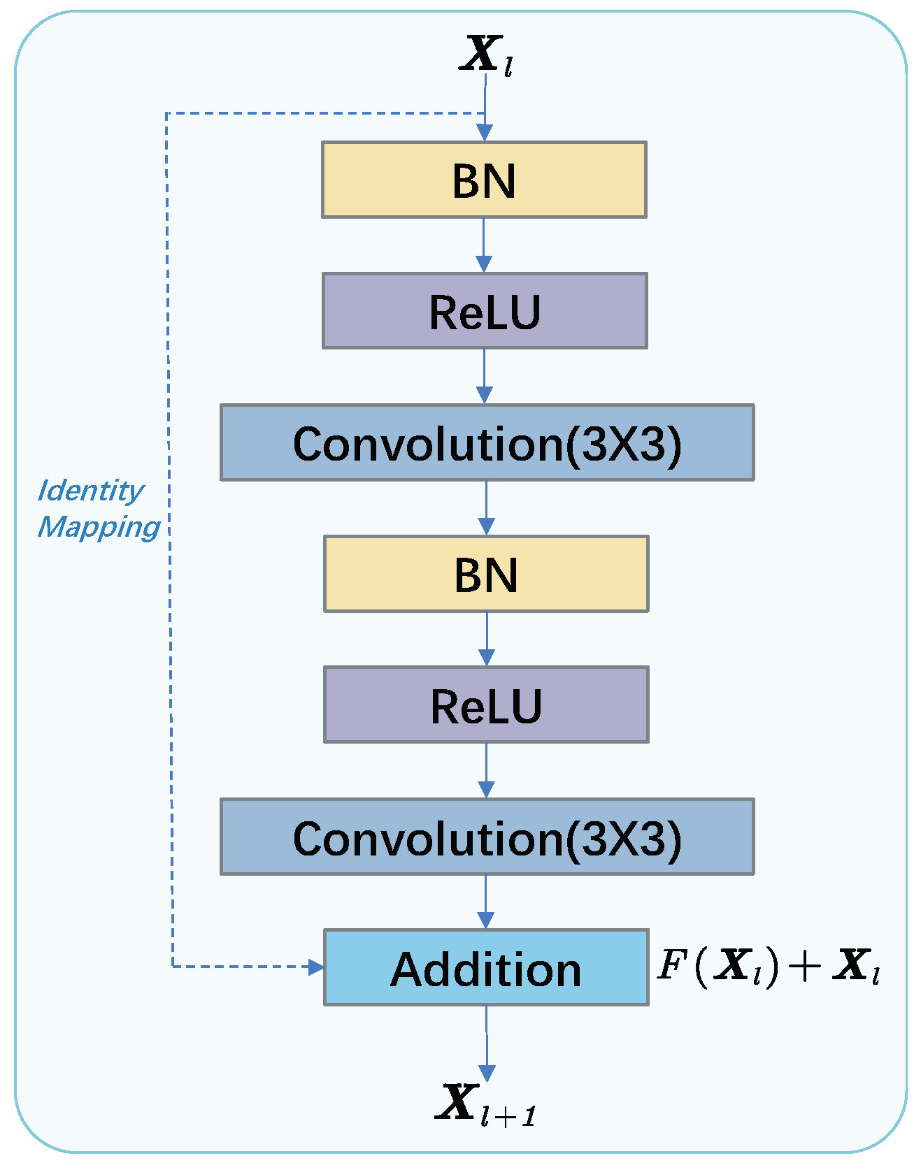
The residual unit and identity mapping used in this work are shown in Figure 3. As the general form of residual units expressed in Equation (12), X l and X l + 1 are input and output of the l-th unit, and F is a residual function and f is a ReLU function.
Y l = h ( X l ) + F ( X l , W l ) , X l + 1 = f ( Y l ) ,
Particularly, the residual unit designed in this work chooses an identity mapping h ( X l ) = X l as suggested in [39]. The identity mapping constructs a direct path for propagating information through the network, which makes the training of our U-Net model in general become easier. So the residual unit can be expressed by Equation (13).
X l + 1 = F ( X l ) + X l
To better suit the U-Net model architecture, each residual unit contains two 3 × 3 convolutions applied repeatedly, each followed by a rectified linear unit (ReLU) and a 2 × 2 max-pooling operation. In addition to this, we also add a batch normalization (BN) [40] unit in front of each round of convolution, which is used to avoid internal covariate shift. This allows the model to apply a higher learning rate as well as avoid the use of dropout to some extent through regularization.

3.3. Dual Attention Module

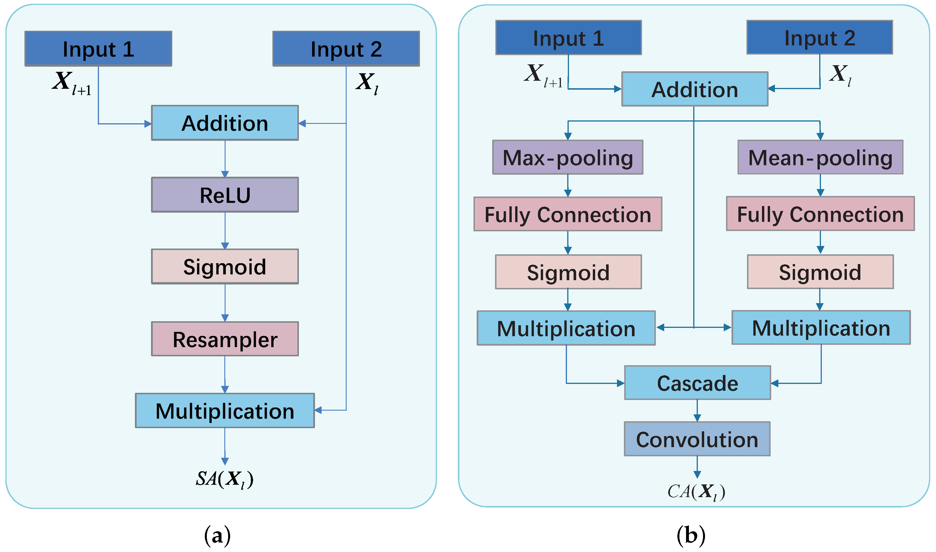
The ground-based MIMO radars and ISAR generally have large imaging scenarios in which there are often several regions of interest and aggregated targets. In this case, it is important to add an attention mechanism to the learning-imaging network that allows the network to focus its limited learning resources on the region where the target is located, rather than the vast background, clutter, or other uninteresting targets. As for the processing of radar imaging data, it is also necessary to add a multi-channel attention mechanism, which will help our model synthesizing the multi-channel information to increase and improve the fault tolerance of the attention mechanism. So, as shown in Figure 4, we explore the addition of a dual-attention mechanism, i.e., the spatial attention module (SA) in Figure 4a and channel attention module (CA) in Figure 4b, to the U-Net model architecture to enhance the convergence speed of the model and the focusing of the imaging results.
As shown in Figure 4, for better integration into the U-Net model architecture, both the CA module and SA module have two inputs, X l and X l + 1 . X l is the output of l-th compression level through concatenation, and X l + 1 is the gating signal from the last extension level. With this design, the dual-attention module inherits the advantages of the concatenation operation in U-Net, which enhances the model’s ability to focus on fine features while applying coarse features to correct them to avoid losing feature information. It can be noticed that the sigmoid activation function was chosen over softmax for both models, the reason being that the sigmoid activation function has better training convergence, whereas the continuous use of the softmax activation function to normalize the attention coefficients produces too sparse activation at the output.

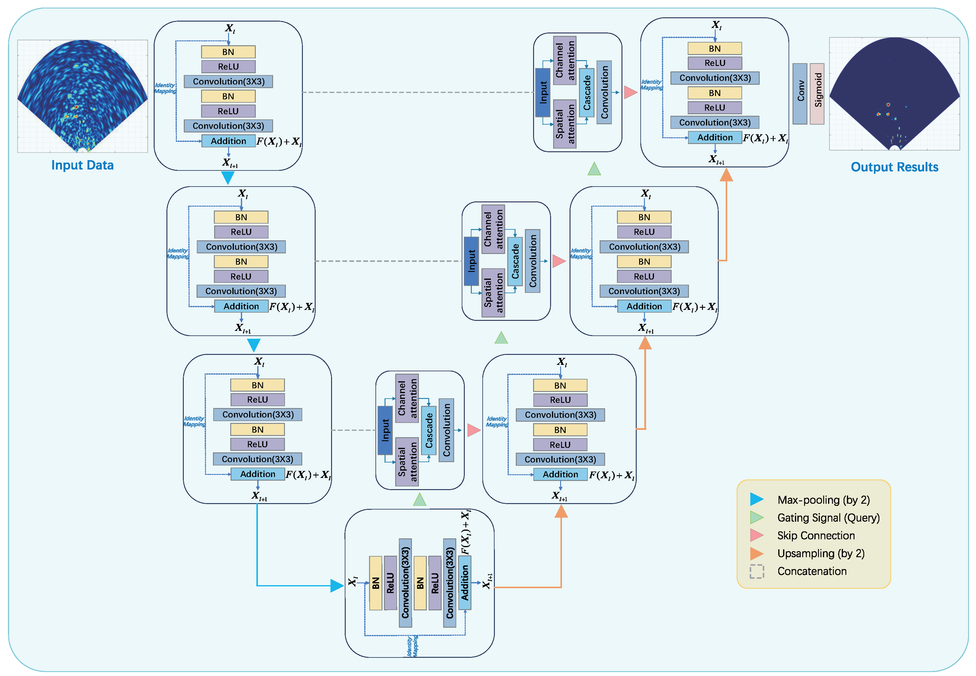
3.4. The Proposed RAU-Net-Based MIMO Radar Imaging Method

Figure 5 illustrates the overall structure of proposed RAU-Net-based MIMO radar imaging method. The model as a whole draws on the structure of the U-Net model to compress and expand the paths, and on this basis, for the MIMO radar imaging scenario, the residual unit and dual attention module are introduced to improve the model. Specifically, (1) the two rounds of convolution in each layer are replaced by a residual unit, which applies the idea of regularization to avoid the dropout and improve the learning efficiency of the model; (2) the dual attention module is added to the concatenation between the two paths, which uses the SA and CA modules to improve the convergence speed and learning efficiency of the model; (3) adding the dual attention module in the concatenation between two paths and cascading the SA and CA modules comprehensively improve the convergence speed of the model learning and enhance the network’s focus on the region of interest.
As can be seen through the model structure diagram in Figure 5, the original image generated by the TCC-BP algorithm is firstly input into the network, and the fine features of the image are gradually learned through the compression path consisting of residual units, while the image information is gradually recovered through the expansion path. In the process of the image passing through the expansion path, each layer is connected with the original information of the image retained by the compression path through concatenation and dual attention module, avoiding the loss of the original information while further enhancing the information of the region of interest. Finally, the network-enhanced imaging results are output after convolution and sigmoid activation function. It is clear to see that the output imaging results have significant improvement effects in target separation, removal of background noise and spatial resolution correction.
The input and output of the model used in this paper are in the form of data matrices, but in order to more intuitively demonstrate the MIMO radar imaging resolution null effect, the imaging results in the paper are temporarily used to show the sector, and the operation process is to plot the model output results in the sector area according to the distance from the radar array and the corresponding compression or expansion. The model input and output size is a 512 × 512 image down each layer of the contraction, and the expansion path image size is halved in the order of 256 2 , 128 2 , 64 2 , 32 2 due to the model of each layer in two convolutions, so the image is input to the edge of the expansion of 2 2 to ensure that each layer of the output image size is the same.

4. Processing Details

In this section, we will specify the operational details of the model, such as data generation methods, model training and model testing strategies.

4.1. Data Acquisition

Table 1 demonstrates the specific parameters for model training. It is widely known that one of the advantages of the U-Net model is the use of less data to achieve model training and convergence. In our model, 500 pairs of training data are selected; the raw data are poor quality imaging results generated by MIMO radar through the TCC-BP algorithm, while the labeled data are generated by selecting the BP algorithm in which the scattering function of the better imaging quality locations is convolved with the imaging locations one by one. In order to improve the noise-resistant performance of the model, 250 sets of data in the datasets were generated under noise-free conditions, and the other 250 sets of data were generated under the condition of −20 dB SNR, and the data were randomly selected in the training datasets to form a batch during the training process. Each data pair is imaged by the MIMO radar on 10-point targets with randomly distributed positions.
During the training process, the training volume of each batch is set to 50 and the learning rate is set to 0.0001 by comparing a large number of training results.The batch size should match the size of the training set, and the learning rate should be determined according to the actual convergence effect of the model. A learning rate that is too small will result in a model that converges too slowly and is prone to generating an overfitted model. A learning rate that is too large will cause the model to converge too quickly, but the model’s ability will not meet expectations.

4.2. Loss Function

Since the proposed model is trained in a supervised manner, the loss function is evaluated using the full reference image evaluation method. The body of the loss function is the mean square error (MSE), which can be calculated by Equation (14), where I i , j is the pixel value of the image at position ( i , j ) .
L M S E = 1 M N i = 1 M j = 1 N ( I i , j m a s k I i , j p r e d i c t i o n ) 2
In addition to the MSE loss, we select the absolute loss L 1 to further reduce the error between the masks and prediction images to obtain a better performance. The L 1 loss can be given as Equation (15).
L 1 = 1 M N m = 1 M n = 1 N | | I i , j m a s k I i , j p r e d i c t i o n | | 1
In ground-based MIMO radar and ISAR imaging scenarios, targets in the region of interest are generally sparse with respect to the entire imaging scene, and also the error matrix should have low rank after removing background noise. So, adding nuclear norm L as the low-rank constraint can enhance the ability of the network to remove the background noise, and L can be calculated with Equation (16) [41].
L = | | I p r e d i c t i o n | |
In the paper [41], the nuclear norm is defined. If a matrix has rank r, then it has exactly r nonzero singular values so that the rank function in the equation below is simply the number of non-vanishing singular values. The sum of the singular values is called the nuclear norm,
| | I p r e d i c t i o n | | = k = 1 n σ k ( I p r e d i c t i o n )
where the σ k ( I p r e d i c t i o n ) denotes the k-th largest singular value of I p r e d i c t i o n .
In summary, the loss function of the model can be synthesized and expressed in the form of Equation (18). In this work, the scaling factor λ of the L 1 is set as λ = 5 3 [28], and the scaling factor η of the L N u c l e a r is set as η = 1 2 .
L G = L M S E + λ L 1 + η L N u c l e a r

4.3. Evaluation Parameter Indicators

In order to quantitatively assess the performance level of the proposed method, three evaluation metrics recognized in the field of image processing are chosen in this chapter to evaluate and score the imaging results: Image Entropy (IE), Image Average Gradient (IAG), and Image Contrast (IC). Since there is no ground truth result for the radar imaging process of the target, this article chooses three non-reference evaluation indexes and combines the scores of the three evaluation indexes to make a comprehensive judgment on the effect of the imaging algorithm.
IE is the statistical form of image features that reflects the amount of average information in an image. In this paper, the two-dimensional entropy of an image is chosen to characterize the spatial features of the image grayscale distribution. Generally speaking, the larger the image entropy is in the absence of noise, the larger the amount of information contained in the image is, i.e., the better the quality of imaging is. The two-dimensional entropy of an image can be calculated with Equation (19), where P i j is the probability of occurrence of a pixel point of a particular value:
I E = i = 0 M j = 0 N P i j log 2 P i j
IAG is the rate of change of the grayscale on both sides of the boundary or shadow line of an image, which reflects the rate of change of the contrast of the tiny details of the image, i.e., the rate of change of the density of the image in the multidimensional direction, and it can be used to characterize the relative sharpness of the image. The average image gradient can be calculated with Equation (20), where I ( i , j ) is the pixel value of the image at position ( i , j ) . In order to better correlate and reflect the enhancement and optimization of the proposed method on the target imaging results, small gradient variations due to background noise or imaging errors are eliminated during the calculation of the IAG. The gradient threshold is set to 0.85 through a large number of experimental statistics, and the real IAG calculation results are enlarged by 10 4 times to facilitate the comparison in the tables:
I A G = 1 ( M 1 ) ( N 1 ) i = 1 M 1 j = 1 N 1 ( I ( i , j ) I ( i + 1 , j ) ) 2 + ( I ( i , j ) I ( i , j + 1 ) ) 2 2 × 10 4
IC is the measure of the difference between the different brightness levels between the light and dark areas in an image. Generally speaking, the higher the contrast is, the more vivid and rich colors the displayed image has. IC can be calculated by the Equation (21), where H is the histogram of input image data. There are various ways of calculating IC in the research of a large number of scholars in the field of computer vision, and we chose the one that is most applicable to the MIMO radar imaging scenario in this paper. Meanwhile, the real calculation results of IC are enlarged by 10 3 times in order to facilitate the comparison display in the tables:
I C = 1 N 1 i = 1 N | H i 1 N i = 1 N H i | 2 × 10 3 , H = i m h i s t ( I m a g e )
Time(s) means the computational time of the comparative algorithms carried on our computer with a CPU of Intel Core i7-12700. As the learning-imaging methods are manipulated on the TCC-BP algorithm, the computational time is a combination format of the TCC-BP algorithm and the relevant learning-imaging method with a ‘+’ between.

5. Experimental Results and Analysis

In this section, we compare the proposed method with three traditional methods and two learning-imaging methods through simulation data experiments and measured data experiments in outdoor scenes, respectively. The results of the comparison experiments prove that the proposed method has obvious advantages in space-variant correction and image denoising. In addition, to illustrate the effectiveness and contribution of the improved parts of the proposed method to improve the imaging performance, we added an ablation experiment at the end.

5.1. Experiments on Simulated Data

To ensure the reference and validity, the simulation experiments adopt the same MIMO radar parameters with the measured experiments as shown in Table 2. Assuming that the radar line-of-sight direction is 0 ° , three point scattering targets are set at ( 45 ° , 50 m), ( 0 ° , 75 m) and ( 45 ° , 100 m) for imaging. Six methods are chosen for the simulation, which are the traditional BP method [12], the TCC-BP method [13], the SVA method [16], the U-Net-based imaging method [22], the GAN-based imaging method [28], and the method proposed in this paper. Additionally, to reduce the sidelobes in the images generated by the BP method and the TCC-BP method, their Hanning-windowed versions are also compared.

5.1.1. Experiment 1: Simulated Targets without Noise

Figure 6 shows the simulated target imaging results under noise-free conditions and Table 3 shows the corresponding performance evaluation indexes. From the imaging results and evaluation indexes, we can find that:
(1)
The traditional BP algorithm in Figure 6a has a high energy aggregation capacity and is conducive to imaging point-scattered targets but has high-level sidelobes;
(2)
By using the Hanning windows, the image sidelobes of the BP algorithm in Figure 6c can be reduced, while the imaging resolution degrades;
(3)
The TCC-BP algorithm in Figure 6b,d has a similar imaging performance to the BP algorithm, but it generates some noisy spots in the image;
(4)
The SVA algorithm in Figure 6e can obtain a sidelobe-reduced image without degrading the imaging resolution, while it causes the deformation and energy spreading in the point spread function edges;
(5)
Although the GAN-based method in Figure 6f can accurately extract the target position information, it cannot remove the sidelobes well, and its imaging quality is relatively poor;
(6)
In the noise-free case, the U-Net-based method in Figure 6g can obtain a close performance to the proposed RAU-Net-based method in Figure 6h, but it has lower IAG and IC performance.
The results shown here demonstrate the imaging quality improvement of the proposed method in the noise-free condition.

5.1.2. Experiment 2: Simulated Targets under −20 dB SNR

Figure 7 shows the simulated target imaging results under the SNR of −20 dB and Table 4 shows the corresponding performance evaluation indexes. From the imaging results and evaluation indexes, we can find that:
(1)
Under strong noise conditions, the BP method in Figure 7a and the TCC-BP method in Figure 7b can only vaguely obtain the locations of targets; the targets almost cannot be automatically identified in the images;
(2)
By using the Hanning windows, the image performance of the BP method in Figure 7c and the TCC-BP method in Figure 7d can be improved but are still much worse than the proposed method;
(3)
The SVA method in Figure 7e has a comparable imaging capability to the Hanning-windowed BP and TCC-BP methods;
(4)
The GAN-based method in Figure 7f is unable to resist the strong noisy environment and its imaged targets are mixed with the background noise;
(5)
The U-Net-based method in Figure 7g and the proposed RAU-net-based method in Figure 7h can clearly separate and identify the targets from the noise, and the latter’s ability of focusing targets and suppressing noise is obviously stronger.
The results shown here demonstrate the imaging quality improvement of the proposed method in the noisy condition.

5.2. Experiments on Outdoor-Scene Measured Data

5.2.1. Introduction to Outdoor Experimental Scene and Targets

In this section, three experiments with real-world measured data are conducted to illustrate the performance and effectiveness of the proposed RAU-Net-based imaging method in practice. Figure 8 shows the MIMO radar system and the experiment scene, where the MIMO array is on the bottom left side and the vector network analyzer (VNA)-based data acquisition equipment is on the bottom right side. Five-type targets in the scene are labeled in Figure 8, which are Building (A), Shrub (B), Trihedral corner reflector (CR)-1 (C), CR-2 (D) and Cars (E). The MIMO array has eight transmitters and eight receivers, which can approximate a virtual aperture of about 1m, giving an azimuth resolution of about 0.03 rad. The VNA is used to generate a stepped frequency continuous wave signal with 481 frequency steps, 5 GHz central frequency, and 150 MHz bandwidth, giving a range resolution of 1 m. Detailed MIMO radar parameters are shown in Table 2.

5.2.2. Experiment 3: Raw Measured Data

Figure 9 shows the imaging results obtained by different methods and Table 5 shows the corresponding performance evaluation indexes. From the imaging results and evaluation indexes, we can find that:
(1)
The images obtained by the BP method in Figure 9a and TCC-BP method in Figure 9b both have obvious spurious signals caused by the sidelobes and background noise, seriously affecting the recognition of targets;
(2)
With the increase of target distance, the azimuth resolution of the BP method and TCC-BP method gradually decreases, which causes an obvious resolution spatial-variant problem, affecting the imaging quality;
(3)
Although the SVA-based method in Figure 9c can significantly reduce the sidelobes and solve the resolution spatial-variant problem to a certain extent, there is still much obvious background noise in the imaging result and a large number of small targets are mixed with the noise, making it difficult to realize effective target recognition;
(4)
The GAN-based imaging method in Figure 9d can extract the target positions and generate their scattering information, but the imaging result only contains a few strong pixels, which greatly reduces the image readability and the amount of information;
(5)
The U-Net-based method in Figure 9e and the proposed RAU-Net-based method in Figure 9f have obvious suppression effects on sidelobes and background noise, and they can better solve the resolution spatial-variant problem.
(6)
By comparing the imaging results and evaluation indexes, it can be obviously found that the proposed RAU-Net-based method can suppress almost all the background noise and perform high-quality imaging of all the five-type targets.

5.2.3. Experiment 4: Measured Data with Additional Gaussian Noise

Figure 10 shows the imaging results by adding Gaussian noise to the measured data and Table 6 shows the corresponding performance evaluation indexes. The way in which the Gaussian noise is added is as follows: assuming that the SNR of the original measured data is S N R o r i g i n and the SNR after adding noise is S N R n o i s y , they satisfy S N R o r i g i n / S N R n o i s y = 20 dB; i.e, the SNR of the measured data has been deteriorated by 20 dB. From the imaging results and evaluation indexes, we can find that:
(1)
Compared to the original results, the BP and TCC-BP imaging results in Figure 10a,b have much more spurious signals caused by the sidelobes and background noise, nearly covering the targets;
(2)
The targets in the image obtained by the SVA-based method in Figure 10c are still almost drowned in noise;
(3)
The targets imaged by the GAN-based imaging method in Figure 10d are more faint and barely noticeable;
(4)
The U-Net-based method in Figure 10e can fully reconstruct the targets, while, as it does not has the attention mechanism and the residual block, it suffers from the energy dispersion on the background noise;
(5)
The proposed RAU-Net-based method in Figure 10f still has obvious suppression effects on sidelobes and background noise in a harsh, noisy environment.

5.2.4. Experiment 5: Measured Data Ablation Experiments with Additional Gaussian Noise

Finally, in Experiment 5, with the same data used in Experiment 4, we conducted ablation experiments on the channel attention block, spatial attention block and residual dense connection block to verify the effect of each proposed module. Figure 11 shows the imaging results and Table 7 shows the corresponding performance evaluation indexes. From the results in Figure 11b,c we can find that the U-Net structure has a significant effect on removing background noise and extracting effective information, while the RD module has a significant contribution to prevent the model from overfitting, i.e., preventing the model from focusing too much energy on background noise. From the result in Figure 11d and the corresponding evaluation indexes, we can corroborate the role of the SA module: without the SA module, although the IE index decreases, the focusing of targets will be greatly reduced, and some weak targets cannot be effectively imaged. Additionally, although the SA block and the CA block both have some effects in improving target focusing and reducing background noise, the role of the SA block is more obvious than the CA block in Figure 11e. In summary, the proposed model and its corresponding modules all contribute to the improvement of imaging performance.

6. Discussion

The model proposed in this article is constructed for spatial-variant correction and denoising in MIMO radar imaging results, and its input and output are images rather than radar data. For the imaging performance, on the one hand, the BP algorithm mainly relies on the coherent superposition of experimental signals for imaging, and the removal of complex domain signals has a limited impact on the imaging quality; on the other hand, from the ablation experiments in the paper, we can find that the channel attention’s contribution to the imaging quality is relatively small, and the selection of complex data will greatly increase the complexity of the model, so the paper selects the RGB three-channel attention mechanism. The proposed network model is a multi-channel real-data model, so the RGB three-channel attention mechanism is selected. However, the complex-valued model needs to be researched further to take advantage of all the information for better imaging performance. Additionally, the labeled data used in this paper are formed by the convolution of a high-resolution BP imaging point spread function at the target location, which has excellent fitting performance to the point scattering target model. The model can also be applied to distributed targets, but it is necessary to replace the labeled data in training with distributed labeled data, and the specific labeled data used should be selected and adjusted properly according to the actual application scenario, which needs to be further investigated in future work.

7. Conclusions

In this article, we propose a RAU-Net-based MIMO radar imaging method that adapts complex noisy scenarios with spatial variation and sidelobe interference. We use the U-Net model as the underlying structure and develop the RAU-Net with two modules: a residual unit with identity mapping and a dual attention module to obtain spatial-variant correction and denoising on real-world MIMO radar images. Combined with the MIMO radar imaging scenario, an improved loss function based on kernel paradigm improvement is proposed, which enhances the network’s ability of focusing for the MIMO radar point spread function and denoising in MIMO radar images. Through training on the constructed simulation datasets, the network can achieve a good generalization ability to the real measurement data of outdoor complex targets, and the network’s ability is verified by multiple rounds of real measurement experiments. The network realizes MIMO radar imaging based on the TCC-BP algorithm, so the total operation time is reduced greatly compared to the traditional BP algorithm on the basis of improving the imaging resolution and denoising capability, ensuring it a wide range of application prospects in the field of real-aperture MIMO radar imaging.

Author Contributions

Conceptualization, J.R. and Y.L.; methodology, J.R.; software, J.R.; validation, J.R., Y.L. and C.F.; formal analysis, Y.L.; investigation, L.S. and H.W.; resources, W.F.; data curation, W.F.; writing—original draft preparation, J.R.; writing—review and editing, J.R., Y.L., W.F. and H.W.; visualization, J.R.; supervision, Y.L., C.F. and L.S.; project administration, Y.L., C.F. and L.S.; funding acquisition, L.S. All authors have read and agreed to the published version of the manuscript.

Funding

This work is supported in part by China Postdoctoral Science Foundation (Grant No. 2021MD703951) and the National Nature Science Foundation of China under Grant 61971434 and Grant 62131020.

Data Availability Statement

Data are contained within the article.

Acknowledgments

We thank the authors of the relevant U-Net methods for making their code open-source so that we can improve our own method and conduct comparative experiments.

Conflicts of Interest

The authors declare no conflicts of interest.

References

  1. Bliss, D.W.; Forsythe, K.W. Multiple-Input Multiple-Output (MIMO) Radar and Imaging: Degrees of Freedom and Resolution. In Proceedings of the Thrity-Seventh Asilomar Conference on Signals, Systems and Computers, Pacific Grove, CA, USA, 9–12 November 2003; pp. 54–59. [Google Scholar] [CrossRef]
  2. Fishler, E.; Haimovich, A.; Blum, R.; Chizhik, D.; Cimini, L.; Valenzuela, R. MIMO Radar: An Idea Whose Time Has Come. In Proceedings of the 2004 IEEE Radar Conference (IEEE Cat. No.04CH37509), Philadelphia, PA, USA, 29 April 2004; pp. 71–78. [Google Scholar] [CrossRef]
  3. Li, J.; Stoica, P. MIMO Radar with Colocated Antennas. IEEE Signal Process. Mag. 2007, 24, 106–114. [Google Scholar] [CrossRef]
  4. Li, J.; Stoica, P.; Zheng, X. Signal Synthesis and Receiver Design for MIMO Radar Imaging. IEEE Trans. Signal Process. 2008, 56, 3959–3968. [Google Scholar] [CrossRef]
  5. Feng, W.; Nico, G.; Guo, J.; Wang, S.; Sato, M. Estimation of Displacement Vector by Linear MIMO Arrays with Reduced System Error Influences. In Proceedings of the IEEE International Geoscience and Remote Sensing Symposium (IGARSS), Yokohama, Japan, 28 July–2 August 2019; pp. 346–349. [Google Scholar]
  6. Zhu, Y.; Su, Y.; Yu, W. An ISAR Imaging Method Based on MIMO Technique. IEEE Trans. Geosci. Remote Sens. 2010, 48, 3290–3299. [Google Scholar] [CrossRef]
  7. Klare, J.; Weiss, M.; Peters, O.; Brenner, A.; Ender, J. ARTINO: A New High Resolution 3D Imaging Radar System on an Autonomous Airborne Platform. In Proceedings of the 2006 IEEE International Symposium on Geoscience and Remote Sensing, Denver, CO, USA, 31 July–4 August 2006; pp. 3842–3845. [Google Scholar] [CrossRef]
  8. Walker, J.L. Range-Doppler Imaging of Rotating Objects. IEEE Trans. Aerosp. Electron. Syst. 1980, AES-16, 23–52. [Google Scholar] [CrossRef]
  9. Milman, A.S.; Milman, A.S. SAR Imaging by ω-K Migration. Int. J. Remote Sens. 1993, 14, 1965–1979. [Google Scholar] [CrossRef]
  10. Carrara, W.G.; Goodman, R.S.; Majewski, R.M. Spotlight Synthetic Radar: Signal Processing Algorithms; Artech House: Boston, MA, USA, 1995. [Google Scholar]
  11. Ulander, L.M.H.; Hellsten, H.; Stenstrom, G. Synthetic-Aperture Radar Processing Using Fast Factorized Back-Projection. IEEE Trans. Aerosp. Electron. Syst. 2003, 39, 760–776. [Google Scholar] [CrossRef]
  12. Wang, H.; Lei, W.; Huang, C.; Su, Y. Mimo Radar Imaging Model and Algorithm. J. Electron. 2009, 26, 577–583. [Google Scholar] [CrossRef]
  13. Wang, H.J.; Huang, C.L.; Lu, M.; Su, Y. Back projection imaging algorithm for MIMO radar. Syst. Eng. Eletron. 2010, 32, 1567–1573. [Google Scholar]
  14. Wang, G.; Lu, Y. Designing Single/multiple Sparse Frequency Waveforms With Sidelobe Constraint. IET Radar Sonar Navig. 2011, 5, 32. [Google Scholar] [CrossRef]
  15. Han, K.; Hong, S. High-Resolution Phased-Subarray MIMO Radar with Grating Lobe Cancellation Technique. IEEE Trans. Microw. Theory Tech. 2022, 70, 2775–2785. [Google Scholar] [CrossRef]
  16. Zhu, R.; Zhou, J.; Fu, Q.; Jiang, G. Spatially Variant Apodization for Grating and Sidelobe Suppression in Near-Range MIMO Array Imaging. IEEE Trans. Microw. Theory Tech. 2020, 68, 4662–4671. [Google Scholar] [CrossRef]
  17. Zhu, R.; Zhou, J.; Jiang, G.; Cheng, B.; Fu, Q. Grating Lobe Suppression in Near Range MIMO Array Imaging Using Zero Migration. IEEE Trans. Microw. Theory Tech. 2020, 68, 387–397. [Google Scholar] [CrossRef]
  18. Noh, H.; Hong, S.; Han, B. Learning Deconvolution Network for Semantic Segmentation. In Proceedings of the 2015 IEEE International Conference on Computer Vision (ICCV), Santiago, Chile, 7–13 December 2015; pp. 1520–1528. [Google Scholar] [CrossRef]
  19. Papandreou, G.; Chen, L.-C.; Murphy, K.P.; Yuille, A.L. Weakly- and Semi-Supervised Learning of a Deep Convolutional Network for Semantic Image Segmentation. In Proceedings of the 2015 IEEE International Conference on Computer Vision (ICCV), Santiago, Chile, 7–13 December 2015; pp. 1742–1750. [Google Scholar] [CrossRef]
  20. Long, J.; Shelhamer, E.; Darrell, T. Fully Convolutional Networks for Semantic Segmentation. In Proceedings of the IEEE Conference on Computer Vision and Pattern Recognition (CVPR), Boston, MA, USA, 7–12 June 2015. [Google Scholar]
  21. Badrinarayanan, V.; Kendall, A.; Cipolla, R. SegNet: A Deep Convolutional Encoder-Decoder Architecture for Image Segmentation. IEEE Trans. Pattern Anal. Mach. Intell. 2017, 39, 2481–2495. [Google Scholar] [CrossRef] [PubMed]
  22. Ronneberger, O.; Fischer, P.; Brox, T. U-Net: Convolutional Networks for Biomedical Image Segmentation. In Medical Image Computing and Computer-Assisted Intervention—MICCAI 2015; Springer: Cham, Switzerland, 2015. [Google Scholar] [CrossRef]
  23. He, K.; Zhang, X.; Ren, S.; Sun, J. Deep Residual Learning for Image Recognition. In Proceedings of the 2016 IEEE Conference on Computer Vision and Pattern Recognition (CVPR), Las Vegas, NV, USA, 27–30 June 2016; pp. 770–778. [Google Scholar] [CrossRef]
  24. Zhang, Z.; Liu, Q.; Wang, Y. Road Extraction by Deep Residual U-Net. IEEE Geosci. Remote Sens. Lett. 2018, 15, 749–753. [Google Scholar] [CrossRef]
  25. Oktay, O.; Schlemper, J.; Folgoc, L.L.; Lee, M.; Heinrich, M.; Misawa, K.; Mori, K.; McDonagh, S.; Hammerla, N.Y.; Kainz, B.; et al. Attention U-Net: Learning Where to Look for the Pancreas. arXiv 2018, arXiv:1804.03999. [Google Scholar] [CrossRef]
  26. Shao, S.; Xiao, L.; Lin, L.; Ren, C.; Ren, C.; Tian, J. Road Extraction Convolutional Neural Network with Embedded Attention Mechanism for Remote Sensing Imagery. Remote Sens. 2022, 14, 2061. [Google Scholar] [CrossRef]
  27. Feng, J.; Jiang, Q.; Tseng, C.H.; Jin, X.; Liu, L.; Zhou, W.; Yao, S. A Deep Multitask Convolutional Neural Network for Remote Sensing Image Super-Resolution and Colorization. IEEE Trans. Geosci. Remote Sens. 2022, 60, 5407915. [Google Scholar] [CrossRef]
  28. Wang, H.; Li, K.; Lu, X.; Zhang, Q.; Luo, Y.; Kang, L. ISAR Resolution Enhancement Method Exploiting Generative Adversarial Network. Remote Sens. 2022, 14, 1291. [Google Scholar] [CrossRef]
  29. Yuan, Y.; Luo, Y.; Ni, J.; Zhang, Q. Inverse Synthetic Aperture Radar Imaging Using an Attention Generative Adversarial Network. Remote Sens. 2022, 14, 3509. [Google Scholar] [CrossRef]
  30. Zhang, Y.; Tian, Y.; Kong, Y.; Zhong, B.; Fu, Y. Residual Dense Network for Image Super-Resolution. arXiv 2018, arXiv:1802.08797. [Google Scholar]
  31. Zhao, S.; Zhang, Z.; Guo, W.; Luo, Y. An Automatic Ship Detection Method Adapting to Different Satellites SAR Images With Feature Alignment and Compensation Loss. IEEE Trans. Geosci. Remote Sens. 2022, 60, 5225217. [Google Scholar] [CrossRef]
  32. Zhang, Y.-P.; Zhang, Q.; Kang, L.; Luo, Y.; Zhang, L. End-to-End Recognition of Similar Space Cone–Cylinder Targets Based on Complex-Valued Coordinate Attention Networks. IEEE Trans. Geosci. Remote Sens. 2022, 60, 5106214. [Google Scholar] [CrossRef]
  33. Shuai, G.; Ting, C.; Penghui, W.; Jun, D.; Junkun, Y.; Yinghua, W.; Hongwei, L. Multistation Cooperative Radar Target Recognition Based on an Angle-Guided Transformer Fusion Network. J. Radars 2023, 12, 516–528. [Google Scholar] [CrossRef]
  34. Xiang, W.; Yumiao, W.; Xingyu, C.; Zang, C.; Cui, G. Deep Learning-Based Marine Target Detection Method with Multiple Feature Fusion. J. Radars 2023, in press. [Google Scholar] [CrossRef]
  35. Zhao, S.; Luo, Y.; Zhang, T.; Guo, W.; Zhang, Z. A Domain Specific Knowledge Extraction Transformer Method for Multisource Satellite-borne SAR Images Ship Detection. ISPRS J. Photogramm. Remote Sens. 2023, 198, 16–29. [Google Scholar] [CrossRef]
  36. Bi, H.; Jin, S.; Wang, X.; Li, Y.; Han, B.; Hong, W. High-resolution High-dimensional Imaging of Urban Building Based on GaoFen-3 SAR Data. J. Radars 2022, 11, 40–51. [Google Scholar] [CrossRef]
  37. Yang, M.; Bai, X.; Wang, L.; Zhou, F. HENC: Hierarchical Embedding Network with Center Calibration for Few-Shot Fine-Grained SAR Target Classification. IEEE Trans. Image Process. 2023, 32, 3324–3337. [Google Scholar] [CrossRef] [PubMed]
  38. Chen, Y.; Wang, S.; Luo, Y.; Liu, H. Measurement Matrix Optimization Based on Target Prior Information for Radar Imaging. IEEE Sensors J. 2023, 23, 9808–9819. [Google Scholar] [CrossRef]
  39. He, K.; Zhang, X.; Ren, S.; Sun, J. Identity Mappings in Deep Residual Networks. In Computer Vision—ECCV 2016; Lecture Notes in Computer, Science; Leibe, B., Matas, J., Sebe, N., Welling, M., Eds.; Springer International Publishing: Cham, Switzerland, 2016; Volume 9908, pp. 630–645. [Google Scholar] [CrossRef]
  40. Ioffe, S.; Szegedy, C. Batch Normalization: Accelerating Deep Network Training by Reducing Internal Covariate Shift. arXiv 2015, arXiv:1502.03167. [Google Scholar] [CrossRef]
  41. Candès, E.J.; Recht, B. Exact Matrix Completion via Convex Optimization. Found. Comput. Math. 2009, 9, 717–772. [Google Scholar] [CrossRef]
Figure 1. Imaging geometry of MIMO array.
Remotesensing 16 00080 g001
Figure 2. Schematic diagram of MIMO array distribution.
Remotesensing 16 00080 g002
Figure 3. Residual unit and identity mapping used in the proposed RAU-Net.
Remotesensing 16 00080 g003
Figure 4. Schematic of the additive dual attention gate used in the proposed RAU-Net. (a) Spatial attention module. (b) Channel attention module.
Remotesensing 16 00080 g004
Figure 5. The architecture of the proposed RAU-Net.
Remotesensing 16 00080 g005
Figure 6. Experiment 1: Imaging results of simulated targets without noise. (a) BP algorithm without Hanning window; (b) TCC-BP algorithm without Hanning window; (c) BP algorithm with Hanning window; (d) TCC-BP algorithm with Hanning window; (e) SVA; (f) GAN; (g) U-Net; (h) ours.
Remotesensing 16 00080 g006aRemotesensing 16 00080 g006b
Figure 7. Experiment 2: Imaging results of simulated targets under −20 dB SNR. (a) BP algorithm without Hanning window; (b) TCC-BP algorithm without Hanning window; (c) BP algorithm with Hanning window; (d) TCC-BP algorithm with Hanning window; (e) SVA; (f) GAN; (g) U-Net; (h) ours.
Remotesensing 16 00080 g007aRemotesensing 16 00080 g007b
Figure 8. Schematic diagram of outdoor experimental scene and targets.
Remotesensing 16 00080 g008
Figure 9. Experiment 3: Imaging results of raw measured data. (a) BP algorithm with Hanning window; (b) TCC-BP algorithm with Hanning window; (c) SVA; (d) GAN; (e) U-Net; (f) ours.
Remotesensing 16 00080 g009aRemotesensing 16 00080 g009b
Figure 10. Experiment 4: Imaging results of measured data with a SNR deterioration of 20 dB. (a) BP algorithm with Hanning window; (b) TCC-BP algorithm with Hanning window; (c) SVA; (d) GAN; (e) U-Net; (f) ours.
Remotesensing 16 00080 g010
Figure 11. Experiment 5: Measured data ablation experiments with with SNR deterioration of 20 dB. (a) TCC-BP algorithm with Hanning window; (b) U-Net; (c) RAU-Net without RD block; (d) RAU-Net without SA block; (e) RAU-Net without CA block; (f) ours.
Remotesensing 16 00080 g011aRemotesensing 16 00080 g011b
Table 1. Training parameters of proposed RAU-Net.
ParametersValue
Noise-free data volume250
−20 dB SNR data volume250
Image size512 × 512
Number of simulation targets10
Batch size50
Learning rate0.0001
CPUIntel Core i7-12700
GPUNVIDIA v100 32 GB
Number of iterations for convergence9500
Training time for convergence118 min 56 s
Table 2. MIMO radar system parameters.
ParametersValue
Start frequency4.925 GHz
Stop frequency5.075 GHz
Number of frequencies481
Number of transmitters/receivers8/8
Range resolution1 m
Azimuth resolution0.03 rad
Length of aperture1 m
Table 3. Experiment 1: Numerical performance evaluation.
Evaluating IndicatorBPTCC-BPBP (hann)TCC-BP (hann)SVAGANU-NetOurs
IE1.3711.4070.5750.5930.5080.2320.3820.284
IAG1.3480.9611.6401.5511.9570.3042.1062.138
IC12.58912.46915.43615.29515.7159.99815.97716.295
Time(s)1.9680.2432.0360.2510.3160.251 + 0.1980.251 + 0.0140.251 + 0.023
Table 4. Experiment 2: Numerical performance evaluation.
Evaluating IndicatorBPTCC-BPBP (hann)TCC-BP (hann)SVAGANU-NetOurs
IE5.8736.1815.4455.4915.414-3.8132.816
IAG0.9700.8701.3721.3231.615-1.6741.966
IC2.0701.7962.4562.4152.483-5.9167.883
Time(s)1.9720.2432.0140.2490.282-0.249 + 0.0140.249 + 0.023
Table 5. Experiment 3: Numerical performance evaluation.
Evaluating IndicatorBP (hann)TCC-BP (hann)SVAGANU-NetOurs
IE4.3964.4224.0531.1881.3841.294
IAG0.6970.6931.1430.7672.2292.363
IC4.2464.1994.76712.08312.94815.108
Time(s)2.2040.2720.4260.272 + 0.1980.272 + 0.0140.272 + 0.023
Table 6. Experiment 4: Numerical performance evaluation.
Evaluating IndicatorBP (hann)TCC-BP (hann)SVAGANU-NetOurs
IE5.0175.0684.6131.3301.4970.858
IAG0.6580.6491.0600.5072.1482.417
IC3.0703.0173.57211.12211.61413.919
Time(s)2.1050.2600.4280.260 + 0.1980.260 + 0.0140.260 + 0.023
Table 7. Experiment 5: Numerical performance evaluation.
Evaluating IndicatorTCC-BP (hann)U-NetRAU-Net without RDRAU-Net without SARAU-Net without CARAU-Net
IE5.0171.4971.4280.8281.3840.858
IAG0.6582.1482.2040.8692.1632.417
IC3.07011.61412.05912.58513.81813.919
Time(s)0.2600.260 + 0.0140.260 + 0.0210.260 + 0.180.260 + 0.0210.260 + 0.023
Disclaimer/Publisher’s Note: The statements, opinions and data contained in all publications are solely those of the individual author(s) and contributor(s) and not of MDPI and/or the editor(s). MDPI and/or the editor(s) disclaim responsibility for any injury to people or property resulting from any ideas, methods, instructions or products referred to in the content.

