Article

Global Terrestrial Evapotranspiration Estimation from Visible Infrared Imaging Radiometer Suite (VIIRS) Data

1
State Key Laboratory of Remote Sensing Science, Faculty of Geographical Science, Beijing Normal University, Beijing 100875, China
2
School of Geography and Environment, Liaocheng University, Liaocheng 252000, China
3
Key Laboratory for Meteorological Disaster Monitoring and Early Warning and Risk Management of Characteristic Agriculture in Arid Regions, CMA, Yinchuan 750002, China
4
Department of Infrastructure Engineering, Faculty of Engineering & IT, University of Melbourne, Melbourne, VIC 3010, Australia
*
Author to whom correspondence should be addressed.
Remote Sens. 2024, 16(1), 44; https://doi.org/10.3390/rs16010044
Submission received: 2 November 2023 / Revised: 6 December 2023 / Accepted: 18 December 2023 / Published: 21 December 2023
(This article belongs to the Special Issue Thermal Remote Sensing for Monitoring Terrestrial Environment)

Abstract

:
It is a difficult undertaking to reliably estimate global terrestrial evapotranspiration (ET) using the Visible Infrared Imaging Radiometer Suite (VIIRS) at high spatial and temporal scales. We employ deep neural networks (DNN) to enhance the estimation of terrestrial ET on a global scale using satellite data. We accomplish this by merging five algorithms that are process-based and that make use of VIIRS data. These include the Shuttleworth–Wallace dual-source ET method (SW), the Priestley–Taylor-based ET algorithm (PT-JPL), the MOD16 ET product algorithm (MOD16), the modified satellite-based Priestley–Taylor ET algorithm (MS-PT), and the simple hybrid ET algorithm (SIM). We used 278 eddy covariance (EC) tower sites from 2012 to 2022 to validate the DNN approach, comparing it to Bayesian model averaging (BMA), gradient boosting regression tree (GBRT) and random forest (RF). The validation results demonstrate that the DNN significantly improves the accuracy of daily ET estimates when compared to three other merging methods, resulting in the highest average determination coefficients (R2, 0.71), RMSE (21.9 W/m2) and Kling–Gupta efficiency (KGE, 0.83). Utilizing the DNN, we generated a VIIRS ET product with a 500 m spatial resolution for the years 2012–2020. The DNN method serves as a foundational approach in the development of a sustained and comprehensive global terrestrial ET dataset. The basis for characterizing and analyzing global hydrological dynamics and carbon cycling is provided by this dataset.

1. Introduction

Terrestrial evapotranspiration (ET) is a crucial component in the intricate interplay of water and carbon exchanges between the hydrological cycle and energy budgets within terrestrial ecosystems [1]. Estimating terrestrial ET accurately presents challenges due to the typically greater heterogeneity of land surfaces compared to sea surfaces, compounded by the uncertainty surrounding intricate biophysical processes [2]. Despite the ability of networks (e.g., FLUXNET) to monitor ET, the absence of data makes it difficult to reliably identify large-scale spatiotemporal ET trends [3].
Satellites are widely recognized as the primary approach for generating global ET products that are distributed in space because they have the ability to accurately measure atmosphere and land surface variables in relation to to variations in ET [4]. Numerous satellite-derived ET products have been accessible since the 1990s, such as the ETMonitor ET product (daily and 1 km) [5]; the Global Land Evaporation Amsterdam Model (GLEAM) version 3 ET product (daily, 0.25°) [6]; the Penman–Monteith–Leuning (PML)_V2 global ET product (8-day, 0.05°) [7,8]; the Global Moderate Resolution Imaging Spectroradiometer (MODIS) ET products (MOD16) (8-day, 500 m) [9,10]; the Breathing Earth System Simulator (BESS) ET product (8-day, 1 km) [11]; the FLUXCOM ET product (8-day, 0.0833°) [12]; and the Global LAnd Surface Satellite (GLASS) ET product Version 5.0 (v5.0) (8-day, 0.05°/1 km) [13]. These products used individual models except for GLASS and FLUXCOM ET products. Previous research has demonstrated that the multi-model merging approach yields superior results compared to any single model when estimating terrestrial ET [14,15,16]. Nevertheless, the performance of the FLUXCOM ET product remains uncertain due to the inherent errors from the FLUXNET sites and in situ observations [17]. Consequently, additional research is required to explore the integration of ET products in order to achieve accurate ET estimations.
Recently, machine learning-based methods have been used to produce ET products by merging ET algorithms. For instance, Yao et al. used the support vector machine method to improve global terrestrial ET estimation by integrating three process-based ET algorithms [18]. Shang et al. merged five satellite-derived products, using extremely randomized trees to estimate terrestrial ET over Europe [19]. By combining five physical models, GLASS ET product v5.0, which has a resolution of 1 km and 8-day, was created as a well-known multi-model ensemble ET product using the deep neural network (DNN) approach [13]. Because DNN has multiple layers of parameterized differentiable nonlinear modules, trained via backpropagation to address a wide range of issues with the large accumulation of satellite and ground observation data, it has been widely used recently to upscale ET from the site to regional scale by relating ground-measured ET to variables derived from satellites and other meteorological data [20,21].
In addition, studies have been carried out to improve the estimation of global terrestrial ET by utilizing the DNN technique, which involves combining multiple satellite-derived ET products. As an illustration, Shang et al. [14] introduced the deep neural network-based merging ET (DNN-MET) framework to enhance the accuracy of ET. The results showed that DNN-MET improved ET estimates over the Heihe River Basin (HRB) and decreased the RMSE by 0.13 to 1.02 mm/day (14–56%) when compared with eight products. Subsequently, the GLASS ET product has been evaluated and validated, and preliminary results indicate that it is of higher quality and accuracy than some of the current satellite-based ET products [22,23]., MODIS has been used as a sensor of the TERRA and AQUA satellites. However, it has been found that the propellant of the accompanying thruster in MODIS becomes exhausted. Subsequently, the GLASS ET products are no longer updated with MODIS products. After 2020, Visible Infrared Imaging Radiometer Suite (VIIRS) was launched and was widely used to retrieve biophysical parameters for product generation. To extend the GLASS ET product after 2020, it is urgent to continue to use VIIRS data to produce ET products.
In the study, we combined five satellite-derived ET algorithms to create a VIIRS ET product using the DNN method from the research. We are aiming to (1) evaluate VIIRS ET algorithm which merges five individual ET algorithms using EC sites from 2012 to 2022; (2) analyze the performance of the DNN in comparison to alternative merging methods (random forest, gradient boosting regression tree, and Bayesian model averaging) at the site level; and (3) produce the VIIRS ET product with a 500 m spatial resolution over the period of 2012–2022, utilizing VIIRS vegetation and GLASS surface net radiation (Rn) datasets, as well as datasets from Modern-Era Retrospective Analysis for Research and Applications, Version 2 (MERRA2).

2. Materials and Methods

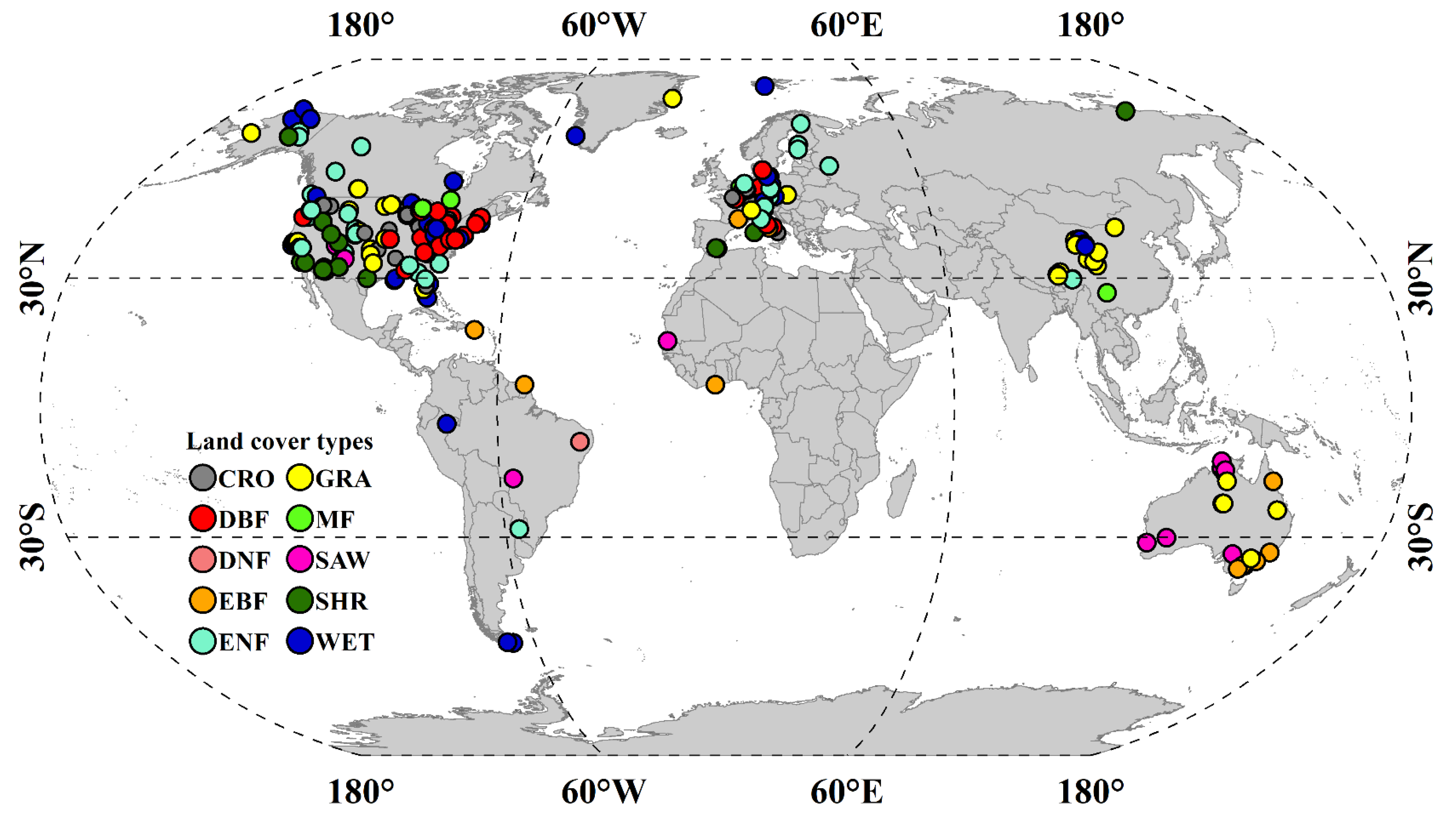
2.1. In Situ Observations

A total 278 eddy covariance (EC) flux tower sites were used, which can be found by referring to Figure 1. Data were gathered from various sources, including AmeriFlux (https://ameriflux.lbl.gov/, last accessed on 20 July 2023), the FLUXNET (https://fluxnet.org/, last accessed on 20 July 2023), the ChinaFLUX National Flux Observation Network (http://www.chinaflux.org/, last accessed on 20 July 2023) and the National Tibetan Plateau Data Center (TPDC, https://data.tpdc.ac.cn/, last accessed on 20 July 2023). The underlying surfaces cover ten plant functional types, croplands (CRO), deciduous broadleaf forests (DBF), deciduous needleleaf forests (DNF), evergreen broadleaf forests (EBF), evergreen needleleaf forests (ENF), grasslands (GRA), mixed forests (MF), savannas (SAW), shrublands (SHR), and wetlands (WET). Before aggregating quality-controlled half-hourly EC observations to obtain daily resolution, we excluded the sensor malfunction data and the incomplete 30 min data from the raw record for the half-hourly and hourly EC observations from every flux tower, and we filled the gaps when data were missing or rejected using the lookup table (LUT) method [24,25]. The Bowen ratio closure method was used to correct the energy imbalance of the original EC observations [26,27].
ET observations from 278 flux tower sites were collected as target variables, and ET values extracted from five ET algorithms (MS-PT, MOD16, SW, PT-JPL and SIM) were used as predictor variables. We assessed the performance of the DNN framework by using a 10-fold cross-validation method. The EC observations were stratified into 10 folds and each fold contained 10% of the EC observations [28]. Entire EC sites were assorted into each fold. The EC sites in each fold were evenly distributed in space. The ET values for each of the 10 parts were estimated based on the trained algorithm by using the remaining nine parts. For each hidden layer in DNN models, we used nodes (2, 4, 8, 16, 32, 64, 128) for random combinations. To reduce the risk of overfitting, we restricted the hidden layers to three (8, 4, and 2) and adopted a ‘rectified linear units’ (ReLU) activation function for the hidden layer.

2.2. Satellite and Meteorological Input to ET Algorithms

In order to assess the performance of ET algorithms across all flux tower sites, we utilized five process-based algorithms driven by four distinct datasets (Table 1). Specifically, we used (1) VIIRS vegetation datasets: fraction of absorbed photosynthetically active radiation (FPAR), leaf area index (LAI), albedo, and normalized difference vegetation index (NDVI) products with a 1 km spatial resolution and 8-day temporal resolution; (2) radiation datasets: the daily Rn with a 0.05° spatial resolution [29]; (3) daily Modern-Era Retrospective Analysis for Research and Applications, Version 2 (MERRA2) datasets: relative humidity (RH), vapor pressure (e), wind spread (WS), air temperature (Ta), soil moisture (SM), and diurnal air temperature range (DT); and a (4) MODIS dataset: land cover. The MERRA2 meteorological data have a spatial resolution of 1/2° × 2/3°. We calculated daily values of FPAR, LAI, and NDVI by temporally interpolating the 8-day averages through the application of the linear interpolation method. Furthermore, we performed a spatial resampling of all MERRA2 and GLASS Rn data at a resolution of 1 km using the bilinear interpolation method.

3. Methods

3.1. Process-Based ET Algorithm

3.1.1. Modified Satellite-Based Priestley–Taylor ET Algorithm (MS-PT)

A modified Priestley–Taylor ET method (MS-PT) based on satellites was designed by Yao et al. [30]. MS-PT divided the total ET into four components: canopy transpiration, vegetation interception evaporation, unsaturated soil evaporation, and saturated wet soil evaporation [30]. The MS-PT algorithm utilizes apparent thermal inertia (ATI), which is determined by the alteration in temperature (Ta, or land surface temperature, LST) over time in order to substitute RH and vapor pressure deficit (VPD) when computing the SM constraint, thus bypassing the challenge of satellite-based estimation of RH and VPD for the PT-JPL algorithm [30]. To simplify the calculation of aerodynamic resistance parameters like PT-JPL, MS-PT only needs Ta, DT derived from MERRA2, Rn from GLASS, and NDVI from VIIRS as inputs.

3.1.2. MODIS ET Product Algorithm (MOD16)

Mu et al. [10] proposed the MODIS ET product algorithm (MOD16) framework using a Penman–Monteith (PM) approach. The MOD16 algorithm has effectively been expanded to produce a MODIS global terrestrial ET dataset based on data inputs, including the leaf area index (LAI), the fraction of absorbed photosynthetically active radiation (FPAR) retrieved from MODIS, and global GMAO meteorological data. The latest MOD16A2 Version 6 global ET product is an 8-day composite dataset and it has too many missing values, limiting continuously spatial and temporal predictions. In addition, the other four ET algorithms employed in this research disregard nighttime ET, unlike the MOD16 ET algorithm, as the majority of ET takes place during the daytime. To ensure consistency, we utilized the MODIS ET algorithm to compute daytime ET, using the average meteorological data for daytime inputs.

3.1.3. Shuttleworth–Wallace Dual Source ET Algorithm (SW)

Shuttleworth and Wallace [31] introduced the Shuttleworth–Wallace dual-source ET algorithm (SW), grounded in energy balance theory. The SW algorithm separated ET into two components: the vegetation transpiration (ETv) and the soil evaporation (ETs). Both ETv and ETs can be estimated using two PM equations when assuming aerodynamic mixing at an average canopy source height. The theoretical enhancement of this model incorporates a composite equation that depicts evaporation by considering the controlling resistances linked with the plants, soil, and water. The equation offers a lucid and conceptually significant depiction of the transition from a barren surface to a thick foliage cover. The input parameters consist of WS, Ta, RH, SM, and e obtained from the MERRA2 dataset, as well as Rn obtained from GLASS and VIIRS LAI.

3.1.4. Priestley–Taylor-Based ET Algorithm (PT-JPL)

Priestley and Taylor [32] proposed a simplified algorithm for estimating ET by attenuating the atmospheric control term in the PM equation and incorporating an empirical factor, avoiding the complexity of parameterizations of both aerodynamic and surface resistance. On the basis of this algorithm, Fisher et al. [33] proposed a novel Piestley–Taylor-based ET equation (PT-JPL). This biometeorological method translates potential ET from the Priestley–Taylor equation into actual ET without using calibration from intensive field measurements [33]. The input variables used to calculate PT-JPL included Ta, and RH derived from MERRA2; Rn derived from GLASS; and NDVI and LAI derived from VIIRS.

3.1.5. Simple Hybrid ET Algorithm (SIM)

Wang and Liang [34] developed a simple hybrid ET algorithm (SIM) based on the Penman equation that combines Rn, NDVI, and Ta. The previous algorithm did not adequately take into account the impact of SM [35]. Therefore, Wang and Liang [34] developed the SIM algorithm, using DT to replace SM in order to further improve ET parameterization. In order to validate the SIM algorithm, extensive analysis was conducted using long-term ground measurements from the Atmospheric Radiation Measurement (ARM)and AmeriFlux sites. The results indicated that the SIM algorithm significantly improved the accuracy of ET estimation when compared to the previous algorithm. The input variables included Ta derived from MERRA2; Rn derived from GLASS; and NDVI derived from VIIRS.

3.2. Machine Learning-Based ET Merging Algorithm

(1)
Deep neural networks (DNN)
Hinton and Salakhutdinov [36] developed the deep neural network (DNN) based on multilayer perceptron (MLP). Compared to MLP, DNN has more layers (ten or more layers) and more effective nonlinear fitting abilities. DNN uses the backpropagation algorithm to optimize model parameters, which is the key factor that improves model training efficiency. DNN’s extensive parameterization makes overfitting a major concern. As a result, we employed the dropout algorithm as a means of preventing overfitting.
(2)
Random forest (RF)
Breiman [37] proposed a random forest (RF) model, which is an ensemble learning algorithm used for classification and regression. The RF model is made up of several decision trees, with each tree trained using a bootstrap sampling algorithm. For the regression task, the result of the RF is the average prediction of the individual decision trees. The RF algorithm, with its ensemble approach, possesses a robust simulation capability and effectively mitigates overfitting.
(3)
Gradient boosting regression tree (GBRT)
Friedman [38] introduced the gradient boosted regression tree (GBRT). GBRT is a boosting regression model that comprises an ensemble of decision trees. This model is constructed in a stage-wise manner and generalizes by optimizing a wide range of loss functions. GBRT possesses the capability to automatically generate suitable nonlinear relationships through the ensemble of trees [39]. Furthermore, GBRT effectively mitigates the issue of overfitting by aggregating numerous weak decision trees. The computational robustness and high scalability exhibited by GBRT positions it as a superior choice when compared to a single decision tree [24].
(4)
Bayesian model averaging (BMA)
Raftery et al. [40] proposed Bayesian model averaging (BMA), which is a statistical probability theory. The BMA establishes a probability density function (PDF) for variables using the weighted average of the individual models’ forecasted probability distributions after correction for bias, weighted by the posterior probability distribution of the corresponding model. The PDF for ET weights each model by its posterior model probabilities and uses the average weights of the PDFs for each model, which may reduce the uncertainties in individual models and thus improve ET accuracy [41].

3.3. Evaluation Metrics

To evaluate the different algorithms against ground measurements, we selected the correlation coefficient of determination (R2) to assess the correlations and adopted the root-mean-square error (RMSE) and bias to quantify the closeness and differences. Moreover, we used the Kling–Gupta efficiency (KGE) [42] to evaluate the overall performance because it incorporates the correlation (r), relative variability ratio ( σ ) and mean value ratio (β) to better understand the mismatches between estimation and observation. The KGE can be written as Equations (1)–(3), where σe and βe are the standard deviation and mean value of estimations, respectively, and σo and βo are those of observations. A KGE nearer to 1 results in improved model performance.
K G E = 1 ( r 1 ) 2 + ( σ 1 ) 2 + ( β 1 ) 2 ,
σ = σ e σ o
β = β e β o

4. Results

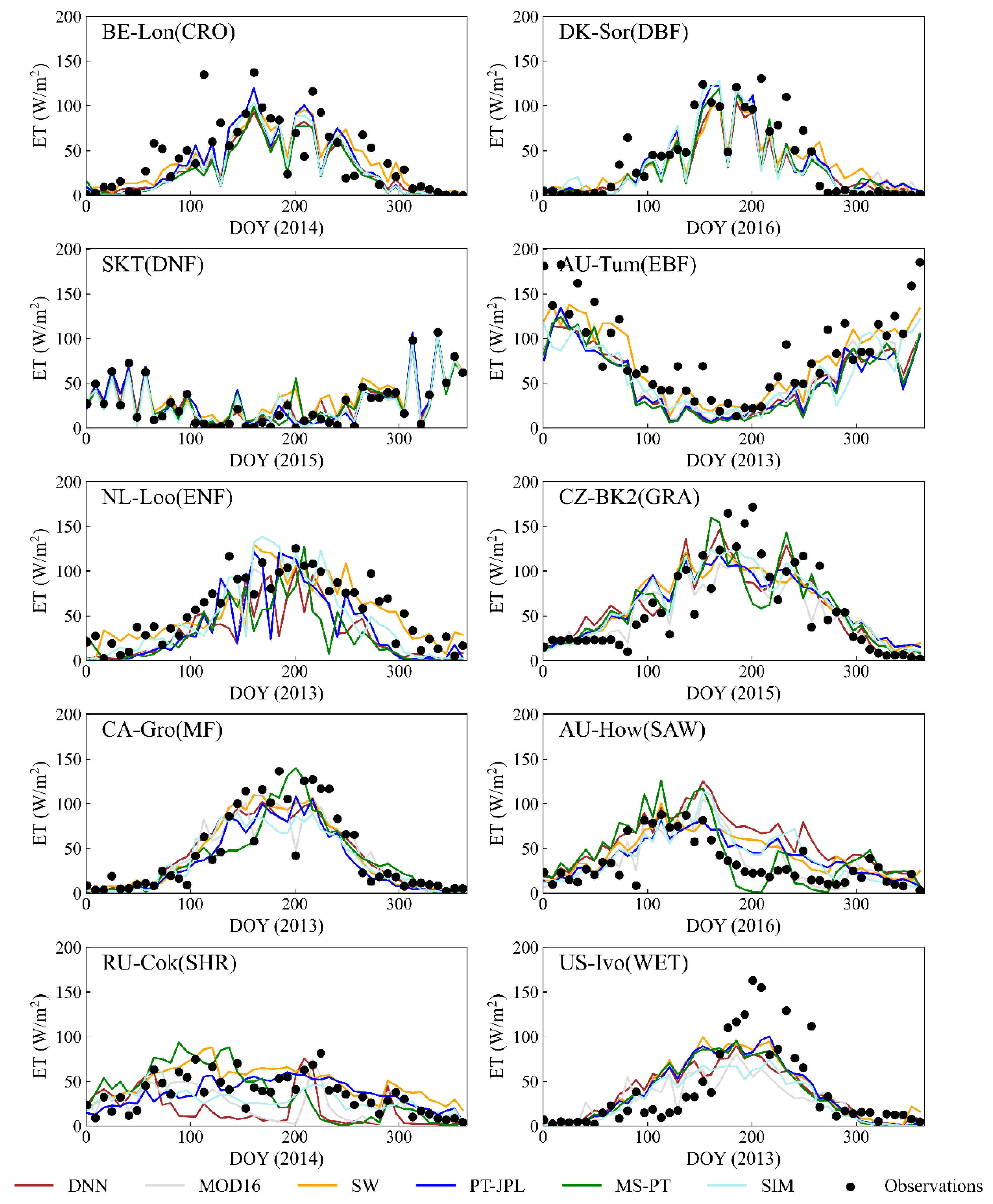
4.1. Evaluation of Five Processed-Based ET Algorithms and DNN

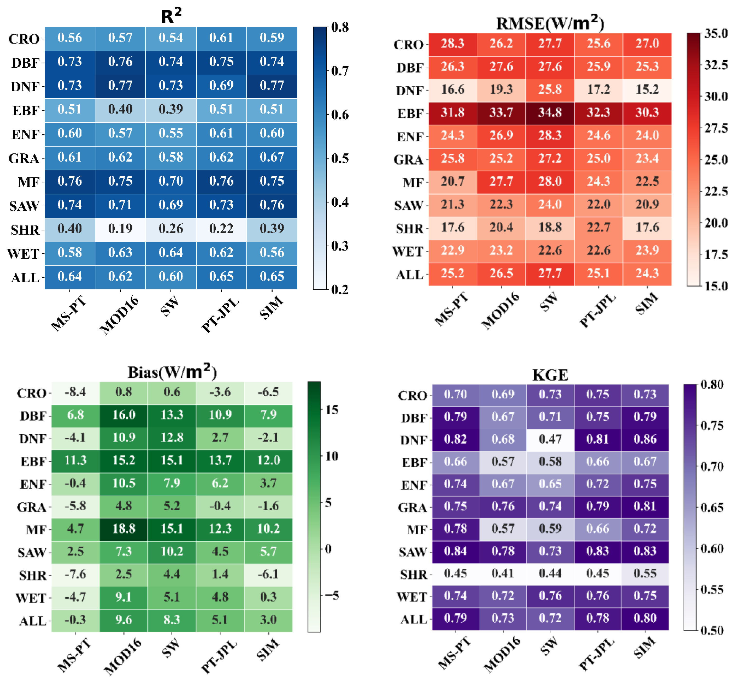
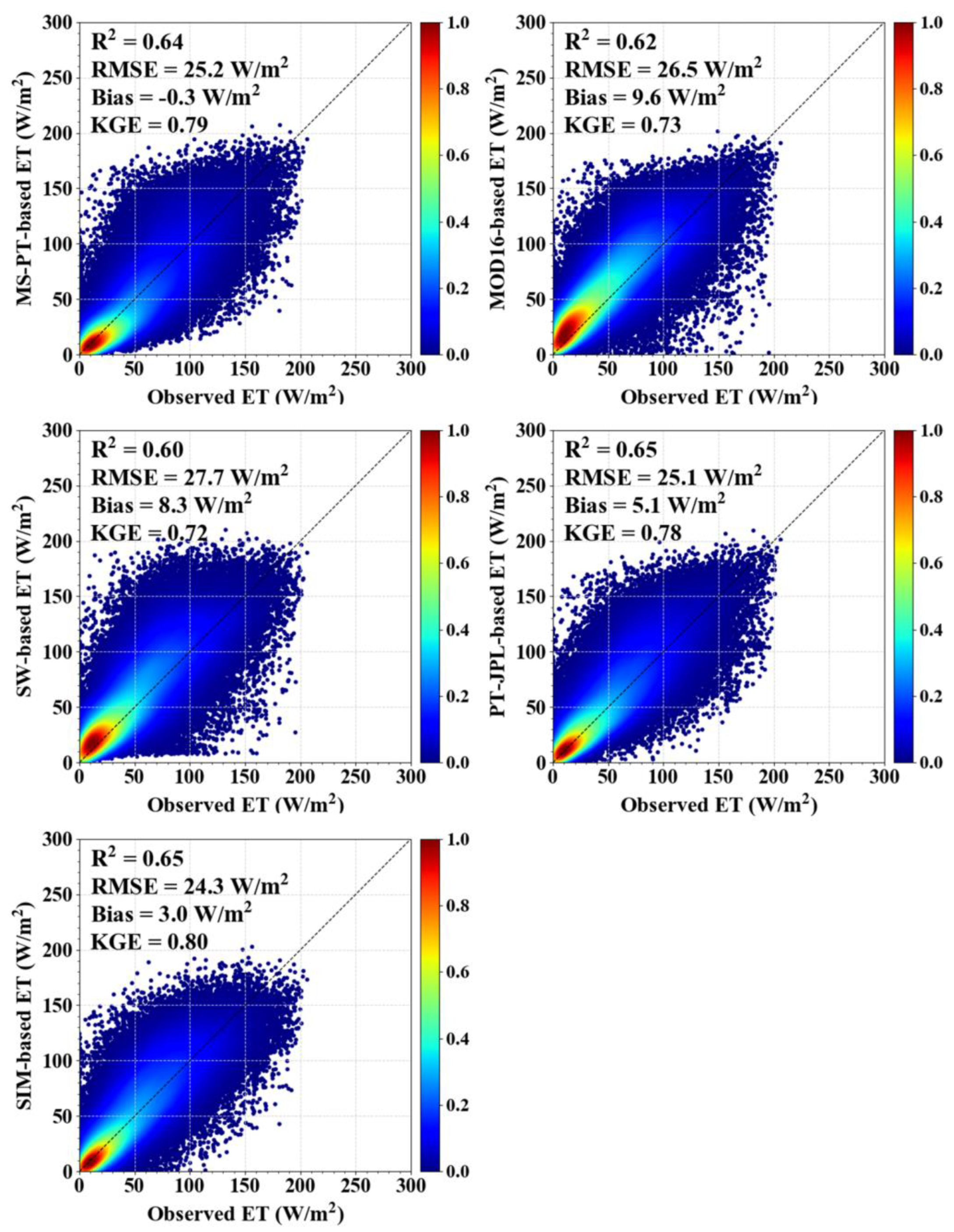
4.1.1. Validation of Five Processed-Based ET Algorithms

Figure 2 shows that the five algorithms exhibit large discrepancies among the different land cover types at the flux tower site scale. The PT-JPL algorithm demonstrates the highest R2 (0.61) and KGE (0.75) values for the CRO flux tower sites, while displaying the lowest RMSE (25.6 W/m2). For the DNF, EBF and GRA flux tower sites, the SIM product has the highest KGE of more than 0.75 and R2 of more than 0.65 (p < 0.01), as well as the lowest RMSE of less than 26 W/m2, compared to the other ET algorithms. The MS-PT algorithm has the highest R2 (0.76) and KGE (0.78) and the lowest RMSE (20.7 W/m2) for MF flux tower sites. For the GRA flux tower sites, the MS-PT product exhibits the smallest RMSE (24 W/m2) and bias (0.6 W/m2). The MS-PT and SIM ET algorithms also exhibit the highest R2 of more than 0.39 (p < 0.01) and KGE of more than 0.45, with a RMSE of less than 17.6 W/m2 for both the SAW and SHR flux tower sites. For the ENF flux tower sites, the SIM algorithm exhibits a smaller RMSE (24.0 W/m2) than the other four ET algorithms. In contrast, the PT-JPL has the highest R2 (0.61, p < 0.01) and the SIM has the highest KGE (0.75). According to the KGE (0.79) and RMSE (15.2 W/m2) values, the accuracy of the SIM ET algorithm is the better than other four algorithms for all of the DBF flux tower sites, but the MOD16 has smaller R2 (0.76, p < 0.01) values. The SW algorithm demonstrates the highest R2 (0.64) and KGE (0.76) values for the WET flux tower sites, while displaying the lowest RMSE (22.6 W/m2). Therefore, we conclude that no single VIIRS-derived ET algorithms can yield the best ET estimation for all land cover types.
Overall, all five processed-based ET algorithms provided reasonable ET estimations for all land cover types, with KGE ranging from 0.72 to 0.80, R2 varying from 0.60 to 0.65 (p < 0.01), bias varying from −0.3 W/m2 to 9.6 W/m2 and RMSE varying from 24.3 W/m2 to 27.1 W/m2 (Figure 3). In terms of performance, the SIM ET algorithm outperforms the PT-JPL, MS-PT, MOD16, and SW ET algorithms, exhibiting the highest KGE and R2 values and the lowest RMSE. Compared with the worst-performing SW algorithm, the SIM reduces the RMSE by 3.4 W/m2 and increases the KGE by approximately 0.8 and R2 by 0.5. In general, the resistance-based ET algorithms (SW and MOD16) have large biases due to complex physical mechanisms and accumulated errors due to excessive numbers of input variables. In contrast, the PT-based ET algorithms (MS-PT and PT-JPL) exhibit higher accuracies in their ET estimations than the SW and RS-PM products, which is due to their partitioning of the total ET and the smaller errors present in the required inputs [43]. Due to the calibration of the SIM ET product using EC ground observations at 15 flux tower sites spanning various land cover types worldwide, it outperforms the other four ET algorithms in terms of ET estimations.

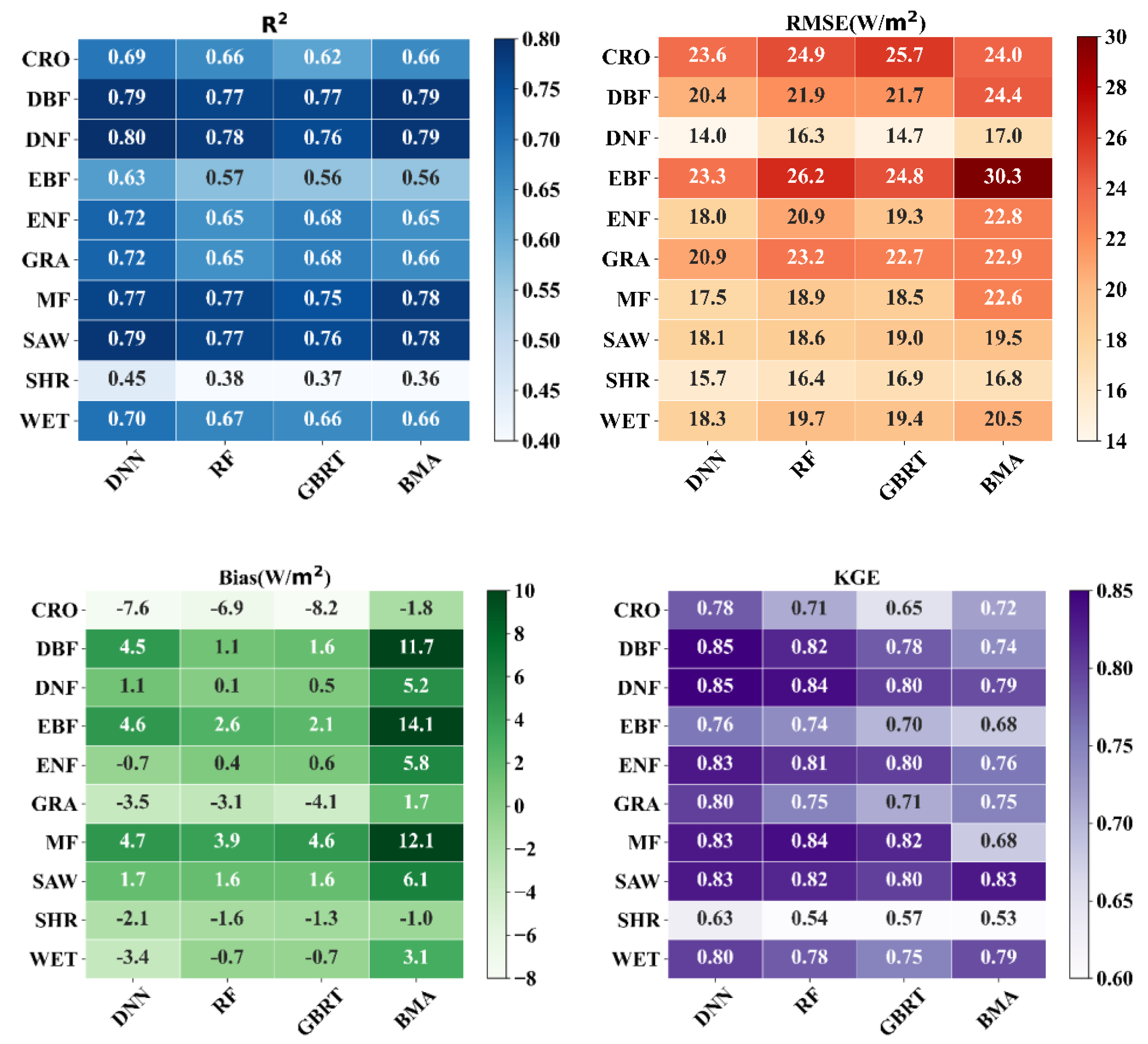
4.1.2. Validation of the DNN

Considering that none of the VIIRS-derived ET algorithms (DNN) can provide an ET estimation across all land cover types that is consistently the best, we used the DNN, RF, GBRT and BMA algorithms to improve the ET estimations by integrating five ET algorithms. Figure 4 shows the performances of the DNN, RF, GBRT and BMA integration algorithms when using the 10-fold cross-validation method for all 278 flux tower sites among all sites. The integration algorithms provide reliable ET estimations, with R2 values ranging from 0.66 to 0.71 (p < 0.01), RMSE values ranging from 21.9 W/m2 to 23.3 W/m2 and KGE values ranging from 0.79 to 0.83. The best performance for ET estimation is provided by the DNN algorithm with the highest R2 (0.71) and KGE (0.83) values and the smallest RMSE (21.9 W/m2) value. This is followed by the GBRT, RF and BMA algorithms.
Figure 5 shows the performances of the DNN, RF, GBRT and BMA integration algorithms when using the 10-fold cross-validation method for different land cover types. The results indicate that the ET estimated using the DNN algorithm for different land cover types displays higher R2 and KGE and lower RMSE values compared to the GBRT, RF and BMA integration algorithms. For the SHR flux tower sites, the DNN algorithm provides better values of KGE of 0.76 and R2 of 0.57 (p < 0.01) and a smaller RMSE of 22.1 W/m2 than the other integration algorithms, although it has the worst performance compared to the other land cover types. For the DNF flux tower sites, the DNN algorithm also exhibits the best capability among all of the integration algorithms, with the highest KGE of 0.63 and R2 of 0.45 (p < 0.01). The DNN algorithm produces highest R2 (0.80, p < 0.01) and KGE (0.85) values, with an RMSE of 14.0 W/m2. This is better than the other integration algorithms for the DNF flux tower sites, and it exhibits better performance than the other land types. Similarly, the DNN algorithm also performs better than the other integration algorithms for the other eight flux tower sites, with an R2 ranging from 0.45–0.80 (p < 0.01), RMSE ranging from 14–23.6 W/m2, and KGE ranging from 0.63–0.85.
Figure 6 shows a time series of the 8-day EC observations and estimated ET from the DNN integration algorithm along with the individual ET algorithms for ten typical land cover types. Compared with the individual ET algorithms, the estimated ET obtained by using the DNN integration algorithm provide obviously seasonal ET curves that are closest to the EC observations. Overall, the errors in the individual ET algorithms are approximately 30%, and the errors in estimated ET based on the DNN algorithm in this study are less than 20%. Therefore, the DNN integration algorithm can be applied to produce ET products with high accuracies at the global scale.

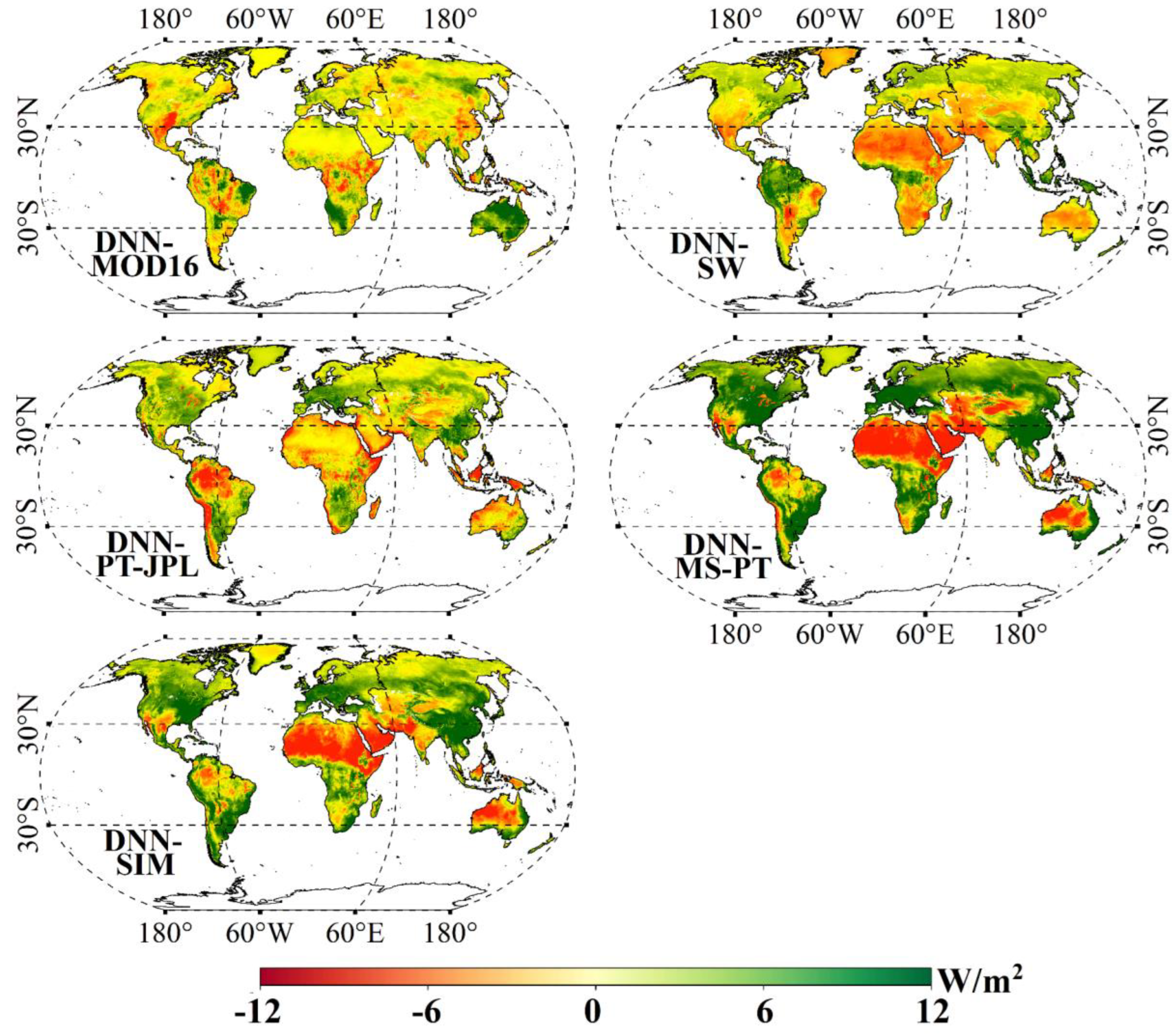
4.2. Mapping of DNN over the Globe

We demonstrated the reliability of the DNN method via comparison with the other five satellite-based algorithms. This validation is particularly challenging due to the limited availability of continuous spatial flux measurements within heterogeneous continental landscapes. We produced a VIIRS product with a spatial resolution of 1 km and temporal resolution of 8 days. Figure 7 displays the spatial pattern of average annual terrestrial ET (2012–2022) for DNN, MOD16, SW, PT-JPL, MS-PT and SIM ET products over the globe. Equatorial regions, such as the rainforests of Amazon, Ituri, and Harapan, exhibit the highest ET for DNN, while high-latitude regions display the lowest ET estimates. The spatial pattern of DNN during 2012–2022 is comparable to that of the other five ET algorithms. The DNN-based product yields a global average annual terrestrial ET (excluding Antarctica) of 37.8 W/m2, which is comparable to the simulated ET values reported in the literature.
The spatial difference in the average annual global terrestrial ET (2012–2022) between DNN and the other five ET algorithms are shown in Figure 8. DNN produces considerably lower ET values compared to other algorithms in tropical regions, while exhibiting higher ET values in North Africa and a section of Australia. The variations in ET estimates in these areas fall within a range of ±8 W/m2. Typically, DNN exhibits minimal spatial disparities in comparison to SIM. In contrast to SW, DNN produces a considerable disparity in space between South America and South Africa. In contrast to PT-JPL and MS-PT, DNN exhibits lower ET values across various regions, such as North Africa, while displaying higher ET values in northwestern Australia. The dissimilarity in space may be attributed to variations in the structures of various ET models.

5. Discussion

5.1. The Performance of DNN

Validation conducted at 278 EC flux tower sites confirms the reliability and robustness of the DNN method in integrating five process-based ET algorithms across land cover types. Figure 4 and Figure 5 both demonstrate that the DNN exhibits negligible bias in ET estimations, delivering results that are closest to the tower flux data compared with the other three merging methods.

5.1.1. The Ability of DNN to Estimate ET

By combining five process-based algorithms, we used the DNN method to generate the VIIRS ET product, which demonstrated its ability to maintain spatiotemporal coherence and generate dependable and resilient estimation for different land cover types. The cross-validations conducted on 278 EC flux tower sites revealed that DNN exhibited superior performance, exhibiting the highest KGE and R2 values, while displaying the lowest RMSE and bias in comparison to other merging methods across different land cover types (Figure 4 and Figure 5). The DNN method exhibited significant variations across biomes and yielded superior results for DBF [KGE of 0.85, R2 of 0.79 (p < 0.01) and RMSE of 20.4 W/m2] and DNF [KGE of 0.85, R2 of 0.80 (p < 0.01) and RMSE of 14.0 W/m2] in comparison to other land cover types. This may be due to the fact that the utilization of vegetation indices or LAI in DNN may account for the seasonal variations in ET for these vegetation types as the robust seasonal nature of satellite vegetation variables (NDVI, FPAR, and LAI) can provide precise insights into the seasonal fluctuations in vegetation [43,44]. Numerous prior studies have reported on various satellite-based ET algorithms, such as the Surface Energy Balance System (SEBS), PT-JPL, and the beta version of MOD16, with the potential to produce more precise ET estimates for vegetation exhibiting substantial seasonal fluctuations (e.g., DBF) [9]. Therefore, by merging these individual ET algorithms that can provide a reasonable seasonality of ET variability, DNN improves the accuracy of ET estimation. In contrast, for some evergreen forests, such as the EBF [KGE of 0.76, R2 of 0.63 (p < 0.01) and RMSE of 27.2 W/m2], DNN yields a relatively poorer estimate. This may be attributed in part to the fact that seasonal EBF variation is less evident [44]. When it comes to CRO, GRA, and SHR flux tower sites, DNN has a tendency to underestimate ET, whereas it has a tendency to overestimate ET for forest flux tower sites. The limitations of the individual ET algorithms can be the primary cause of this. The enhancement of DNN was further validated through a sequence of validations utilizing EC observations. Generally, BMA showed worse accuracy than the other three methods. The BMA’s inability to effectively fit nonlinear input data may be partly due to the implementation of multilayer learning [45]. Moreover, the DNN outperforms the GBRT, RF and BMA when it comes to transforming input data and achieving a depth of tens/hundreds of multiple layers, resulting in significant time and effort savings [44].

5.1.2. The Uncertainties of DNN Estimate

Although DNN improved the accuracy of ET estimations, there are still uncertainties and errors in ET estimates, including the data sources, the spatial scale mismatch between flux tower sites and satellite pixels, and the algorithm structure of DNN [9,46].
The inaccuracies of data sources are predominantly passed down through in situ measurements, satellite-based observations, and meteorological reanalysis data. Although EC observations are relatively accurate for ET acquisition, biases of approximately 5–25% still exist [26]. The EC method’s major drawback lies in its energy imbalance and inability to detect large eddies. Although we corrected the energy imbalance using a method developed by Twine et al. (2000) [27], the uncertainties in EC observations remain unclear [47]. Previous studies showed that MERRA2 meteorological data also contain a large bias when compared to in situ measurements, and no single reanalysis dataset is superior to others in terms of meteorological variables in terms of estimating land surface energy budgets [48,49].
The mismatched spatial scales between in situ measurements and satellite observations may cause large uncertainties [50,51]. Additionally, we used MERRA2 products with a spatial resolution of 1/2° × 2/3°. These were resampled spatially into 500 m using the bilinear interpolation method. However, the resolution of MRERRA2 is greater than the footprint for field measurements [48]. Thus, accurate meteorological information for flux tower sites cannot be acquired due to their coarse spatial resolution and errors in the bilinear interpolation method [52]. Therefore, the issue of errors caused by scaling effects is also significant.
Different ET model structures lead to a 20% bias in ET estimation [53]. Despite the strength of the DNN model, its performance is typically determined by the representation of training data. The 278 EC sites used in the study are sparsely distributed and cover limited land surfaces around the world, failing to cover the full globe. The lack of a sufficient quantity of labeled data could lead to DNN displaying an inferior performance [54]. Therefore, the errors in the training samples could lead to the inheritance of uncertainties. Furthermore, DNN uses numerous hyperparameters as input and requires precise tuning in order to produce a beneficial learning outcome [55]. Moreover, an excessive number of disruptive elements could certainly bring about considerable unpredictability in the process of constructing the model [55].

5.2. Advantages and Limitations of DNN

The DNN model is powerful, and it has distinct advantages. DNN can accurately approximate the complicated nonlinear relationship between observed EC and ET estimates using multilayer learning, which helps to capture the potential association between different variables for the spatiotemporal fusion of remote sensing data [56]. Research has demonstrated that DNN is able to incorporate multiple ecological variables into their predictions, which could lead to more precise ET estimates [14,56]. Additionally, DNN preserves some physical mechanisms of individual algorithms for producing the individual ET products and can better simulate ET under extreme conditions than pure machine learning. This is because fusion models can merge the information provided by different sources to improve algorithm performance as well as provide a better physical interpretation of the results to enhance the understanding of ET processes [57].
Nonetheless, DNNs possess comparable limitations to other forms of machine learning methods. Initially, a DNN’s intricate neural network architecture necessitates a substantial amount of training data, thus constraining its effectiveness on smaller data sets [58]. However, DNN would not perform as well if there was not enough labeled data. Furthermore, the inclusion of multiple ET algorithms with different meteorological inputs in the model, as well as the possibility of incorporating irrelevant interfering factors and a wide range of possible configurations, could increase the level of uncertainty associated with model construction [55]. Typically, deep neural networks necessitate numerous hyperparameters, and the effectiveness of DNN is heavily reliant on their parameter adjustment, thereby diminishing the efficiency of ET algorithm generation [54].

6. Conclusions

We used the DNN method to produce VIIRS ET product by merging five satellite-derived ET algorithms and 278 globally distributed flux towers from 2012–2022. The main findings are as follows:
(1)
There is no single VIIRS-derived ET algorithms that can yield the best ET estimations for all land cover types.
(2)
DNN has spatial consistency and relatively lower uncertainty with the highest R2 (0.71), RMSE (21.9 W/m2) and KGE (0.83) outperformed other merging methods (RF, GBRT and BMA) and five individual process-based ET algorithms (SIM, MS-PT, PT-JPL, MOD16 and SW).

Author Contributions

Conceptualization, Q.T. and Y.Y.; methodology, Z.X.; software, X.Z. (Xiaotong Zhang); validation, Z.X. and B.J.; formal analysis, J.X. and X.Z. (Xueyi Zhang); investigation, R.Y.; resources, L.L.; data curation, J.N.; writing—original draft preparation, Z.X.; writing—review and editing, Y.Y.; visualization, J.F.; supervision, L.Z.; project administration, Y.Y.; funding acquisition, Y.Y. All authors have read and agreed to the published version of the manuscript.

Funding

This research was funded by the Natural Science Fund of China (No. 42192581 and No. 42171310). This research was also supported by the Open Research Program of the International Research Center of Big Data for Sustainable Development Goals (No. CBAS2022ORP01).

Data Availability Statement

The data presented in this study are available on request from the corresponding author. The data are not publicly available due to privacy.

Conflicts of Interest

The authors declare no conflict of interest.

References

  1. Wang, K.C.; Dickinson, R.E. A review of global terrestrial evapotranspiration: Observation, modeling, climatology, and climatic variability. Rev. Geophys. 2012, 50. [Google Scholar] [CrossRef]
  2. Kool, D.; Agam, N.; Lazarovitch, N.; Heitman, J.L.; Sauer, T.J.; Ben-Gal, A. A review of approaches for evapotranspiration partitioning. Agric. For. Meteorol. 2014, 184, 56–70. [Google Scholar] [CrossRef]
  3. Baldocchi, D.; Falge, E.; Gu, L.H.; Olson, R.; Hollinger, D.; Running, S.; Anthoni, P.; Bernhofer, C.; Davis, K.; Evans, R.; et al. Fluxnet: A new tool to study the temporal and spatial variability of ecosystem-scale carbon dioxide, water vapor, and energy flux densities. Bull. Am. Meteorol. Soc. 2001, 82, 2415–2434. [Google Scholar] [CrossRef]
  4. Brust, C.; Kimball, J.S.; Maneta, M.P.; Jencso, K.; He, M.Z.; Reichle, R.H. Using smap level-4 soil moisture to constrain mod16 evapotranspiration over the contiguous USA. Remote Sens. Environ. 2021, 255, 112277. [Google Scholar] [CrossRef]
  5. Hu, G.C.; Jia, L. Monitoring of evapotranspiration in a semi-arid inland river basin by combining microwave and optical remote sensing observations. Remote Sens. 2015, 7, 3056–3087. [Google Scholar] [CrossRef]
  6. Martens, B.; Miralles, D.G.; Lievens, H.; van der Schalie, R.; de Jeu, R.A.M.; Fernández-Prieto, D.; Beck, H.E.; Dorigo, W.A.; Verhoest, N.E.C. Gleam v3: Satellite-based land evaporation and root-zone soil moisture. Geosci. Model Dev. 2017, 10, 1903–1925. [Google Scholar] [CrossRef]
  7. Zhang, Y.Q.; Kong, D.D.; Gan, R.; Chiew, F.H.S.; McVicar, T.R.; Zhang, Q.; Yang, Y.T. Coupled estimation of 500 m and 8-day resolution global evapotranspiration and gross primary production in 2002–2017. Remote Sens. Environ. 2019, 222, 165–182. [Google Scholar] [CrossRef]
  8. Zhang, Y.Q.; Pena-Arancibia, J.L.; McVicar, T.R.; Chiew, F.H.S.; Vaze, J.; Liu, C.M.; Lu, X.J.; Zheng, H.X.; Wang, Y.P.; Liu, Y.Y.; et al. Multi-decadal trends in global terrestrial evapotranspiration and its components. Sci. Rep. 2016, 6, 19124. [Google Scholar] [CrossRef]
  9. Mu, Q.; Heinsch, F.A.; Zhao, M.; Running, S.W. Development of a global evapotranspiration algorithm based on modis and global meteorology data. Remote Sens. Environ. 2007, 111, 519–536. [Google Scholar] [CrossRef]
  10. Mu, Q.Z.; Zhao, M.S.; Running, S.W. Improvements to a modis global terrestrial evapotranspiration algorithm. Remote Sens. Environ. 2011, 115, 1781–1800. [Google Scholar] [CrossRef]
  11. Jiang, C.; Ryu, Y. Multi-scale evaluation of global gross primary productivity and evapotranspiration products derived from breathing earth system simulator (bess). Remote Sens. Environ. 2016, 186, 528–547. [Google Scholar] [CrossRef]
  12. Jung, M.; Koirala, S.; Weber, U.; Ichii, K.; Gans, F.; Camps-Valls, G.; Papale, D.; Schwalm, C.; Tramontana, G.; Reichstein, M. The fluxcom ensemble of global land-atmosphere energy fluxes. Sci. Data 2019, 6, 74. [Google Scholar] [CrossRef] [PubMed]
  13. Xie, Z.J.; Yao, Y.J.; Zhang, X.T.; Liang, S.L.; Fisher, J.B.; Chen, J.Q.; Jia, K.; Shang, K.; Yang, J.M.; Yu, R.Y.; et al. The global land surface satellite (glass) evapotranspiration product version 5.0: Algorithm development and preliminary validation. J. Hydrol. 2022, 610, 127990. [Google Scholar] [CrossRef]
  14. Shang, K.; Yao, Y.J.; Liang, S.L.; Zhang, Y.H.; Fisher, J.B.; Chen, J.Q.; Liu, S.M.; Xu, Z.W.; Zhang, Y.; Jia, K.; et al. Dnn-met: A deep neural networks method to integrate satellite-derived evapotranspiration products, eddy covariance observations and ancillary information. Agric. For. Meteorol. 2021, 308, 108582. [Google Scholar] [CrossRef]
  15. Mueller, B.; Hirschi, M.; Jimenez, C.; Ciais, P.; Dirmeyer, P.A.; Dolman, A.J.; Fisher, J.B.; Jung, M.; Ludwig, F.; Maignan, F.; et al. Benchmark products for land evapotranspiration: Landflux-eval multi-data set synthesis. Hydrol. Earth Syst. Sci. 2013, 17, 3707–3720. [Google Scholar] [CrossRef]
  16. Jiménez, C.; Martens, B.; Miralles, D.M.; Fisher, J.B.; Beck, H.E.; Fernández-Prieto, D. Exploring the merging of the global land evaporation wacmos-et products based on local tower measurements. Hydrol. Earth Syst. Sci. 2018, 22, 4513–4533. [Google Scholar] [CrossRef]
  17. Ma, N.; Szilagyi, J.; Jozsa, J. Benchmarking large-scale evapotranspiration estimates: A perspective from a calibration-free complementary relationship approach and fluxcom. J. Hydrol. 2020, 590, 125221. [Google Scholar] [CrossRef]
  18. Yao, Y.Y.; Liang, S.L.; Li, X.L.; Chen, J.Q.; Liu, S.M.; Jia, K.; Zhang, X.T.; Xiao, Z.Q.; Fisher, J.B.; Mu, Q.Z.; et al. Improving global terrestrial evapotranspiration estimation using support vector machine by integrating three process-based algorithms. Agric. For. Meteorol. 2017, 242, 55–74. [Google Scholar] [CrossRef]
  19. Shang, K.; Yao, Y.J.; Li, Y.F.; Yang, J.M.; Jia, K.; Zhang, X.T.; Chen, X.W.; Bei, X.Y.; Guo, X.Z. Fusion of five satellite-derived products using extremely randomized trees to estimate terrestrial latent heat flux over europe. Remote Sens. 2020, 12, 687. [Google Scholar] [CrossRef]
  20. Chollet, F. Deep Learning with Python; Manning Publications: Shelter Island, NY, USA, 2017; pp. 1800–1807. [Google Scholar]
  21. Ienco, D.; Interdonato, R.; Gaetano, R.; Minh, D.H.T. Combining sentinel-1 and sentinel-2 satellite image time series for land cover mapping via a multi-source deep learning architecture. Isprs. J. Photogramm. 2019, 158, 11–22. [Google Scholar] [CrossRef]
  22. Yang, L.S.; Feng, Q.; Zhu, M.; Wang, L.M.; Alizadeh, M.R.; Adamowski, J.F.; Wen, X.H.; Yin, Z.L. Variation in actual evapotranspiration and its ties to climate change and vegetation dynamics in northwest China. J. Hydrol. 2022, 607, 127533. [Google Scholar] [CrossRef]
  23. Song, L.S.; Liu, S.M.; Kustas, W.P.; Nieto, H.; Sun, L.; Xu, Z.W.; Skaggs, T.H.; Yang, Y.; Ma, M.G.; Xu, T.R.; et al. Monitoring and validating spatially and temporally continuous daily evaporation and transpiration at river basin scale. Remote Sens. Environ. 2018, 219, 72–88. [Google Scholar] [CrossRef]
  24. Yao, Y.J.; Liang, S.L.; Li, X.L.; Chen, J.Q.; Wang, K.C.; Jia, K.; Cheng, J.; Jiang, B.; Fisher, J.B.; Mu, Q.Z.; et al. A satellite-based hybrid algorithm to determine the priestley-taylor parameter for global terrestrial latent heat flux estimation across multiple biomes (vol 165, pg 216, 2015). Remote Sens. Environ. 2015, 169, 454. [Google Scholar] [CrossRef]
  25. Falge, E.; Baldocchi, D.; Olson, R.; Anthoni, P.; Aubinet, M.; Bernhofer, C.; Burba, G.; Ceulemans, R.; Clement, R.; Dolman, H.; et al. Gap filling strategies for defensible annual sums of net ecosystem exchange. Agric. For. Meteorol. 2001, 107, 43–69. [Google Scholar] [CrossRef]
  26. Foken, T. The energy balance closure problem: An overview. Ecol. Appl. 2008, 18, 1351–1367. [Google Scholar] [CrossRef] [PubMed]
  27. Twine, T.E.; Kustas, W.P.; Norman, J.M.; Cook, D.R.; Houser, P.R.; Meyers, T.P.; Prueger, J.H.; Starks, P.J.; Wesely, M.L. Correcting eddy-covariance flux underestimates over a grassland. Agric. For. Meteorol. 2000, 103, 279–300. [Google Scholar] [CrossRef]
  28. Jung, M.; Reichstein, M.; Margolis, H.A.; Cescatti, A.; Richardson, A.D.; Arain, M.A.; Arneth, A.; Bernhofer, C.; Bonal, D.; Chen, J.Q.; et al. Global patterns of land-atmosphere fluxes of carbon dioxide, latent heat, and sensible heat derived from eddy covariance, satellite, and meteorological observations. J. Geophys. Res.-Biogeosci. 2011, 116, G3. [Google Scholar] [CrossRef]
  29. Jiang, B.; Zhang, Y.; Liang, S.L.; Wohlfahrt, G.; Arain, A.; Cescatti, A.; Georgiadis, T.; Jia, K.; Kiely, G.; Lund, M.; et al. Empirical estimation of daytime net radiation from shortwave radiation and ancillary information. Agric. For. Meteorol. 2015, 211, 23–36. [Google Scholar] [CrossRef]
  30. Yao, Y.J.; Liang, S.L.; Cheng, J.; Liu, S.M.; Fisher, J.B.; Zhang, X.D.; Jia, K.; Zhao, X.; Qing, Q.M.; Zhao, B.; et al. Modis-driven estimation of terrestrial latent heat flux in China based on a modified priestley-taylor algorithm. Agric. For. Meteorol. 2013, 171, 187–202. [Google Scholar] [CrossRef]
  31. Shuttleworth, W.J.; Wallace, J.S. Evaporation from sparse crops—An energy combination theory. Q. J. Roy. Meteor. Soc. 1985, 111, 839–855. [Google Scholar] [CrossRef]
  32. Priestley, C.H.B.; Taylor, R.J. On the assessment of surface heat flux and evaporation using large scale parameters. Mon. Weather. Rev. 1972, 100, 81–92. [Google Scholar] [CrossRef]
  33. Fisher, J.B.; Tu, K.P.; Baldocchi, D.D. Global estimates of the land-atmosphere water flux based on monthly avhrr and islscp-ii data, validated at 16 fluxnet sites. Remote Sens. Environ. 2008, 112, 901–919. [Google Scholar] [CrossRef]
  34. Wang, K.C.; Liang, S.L. An improved method for estimating global evapotranspiration based on satellite determination of surface net radiation, vegetation index, temperature, and soil moisture. J. Hydrometeorol. 2008, 9, 712–727. [Google Scholar] [CrossRef]
  35. Wang, K.C.; Wang, P.; Li, Z.Q.; Cribb, M.; Sparrow, M. A simple method to estimate actual evapotranspiration from a combination of net radiation, vegetation index, and temperature. J. Geophys. Res.-Atmos. 2007, 112, D15. [Google Scholar] [CrossRef]
  36. Hinton, G.E.; Salakhutdinov, R.R. Reducing the dimensionality of data with neural networks. Science 2006, 313, 504–507. [Google Scholar] [CrossRef] [PubMed]
  37. Breiman, L. Random forests. Mach. Learn. 2001, 45, 5–32. [Google Scholar] [CrossRef]
  38. Friedman, J.H. Greedy function approximation: A gradient boosting machine. Ann. Stat. 2001, 29, 1189–1232. [Google Scholar] [CrossRef]
  39. Wei, Y.; Zhang, X.T.; Hou, N.; Zhang, W.Y.; Jia, K.; Yao, Y.J. Estimation of surface downward shortwave radiation over China from avhrr data based on four machine learning methods. Sol. Energy 2019, 177, 32–46. [Google Scholar] [CrossRef]
  40. Raftery, A.E.; Madigan, D.; Hoeting, J.A. Bayesian model averaging for linear regression models. J. Am. Stat. Assoc. 1997, 92, 179–191. [Google Scholar] [CrossRef]
  41. Chen, Y.; Yuan, W.P.; Xia, J.Z.; Fisher, J.B.; Dong, W.J.; Zhang, X.T.; Liang, S.L.; Ye, A.Z.; Cai, W.W.; Feng, J.M. Using bayesian model averaging to estimate terrestrial evapotranspiration in China. J. Hydrol. 2015, 528, 537–549. [Google Scholar] [CrossRef]
  42. Gupta, H.V.; Kling, H.; Yilmaz, K.K.; Martinez, G.F. Decomposition of the mean squared error and nse performance criteria: Implications for improving hydrological modelling. J. Hydrol. 2009, 377, 80–91. [Google Scholar] [CrossRef]
  43. Ershadi, A.; McCabe, M.F.; Evans, J.P.; Chaney, N.W.; Wood, E.F. Multi-site evaluation of terrestrial evaporation models using fluxnet data. Agric. For. Meteorol. 2014, 187, 46–61. [Google Scholar] [CrossRef]
  44. Yebra, M.; Van Dijk, A.; Leuning, R.; Huete, A.; Guerschman, J.P. Evaluation of optical remote sensing to estimate actual evapotranspiration and canopy conductance. Remote Sens. Environ. 2013, 129, 250–261. [Google Scholar] [CrossRef]
  45. Duan, Q.Y.; Ajami, N.K.; Gao, X.G.; Sorooshian, S. Multi-model ensemble hydrologic prediction using bayesian model averaging. Adv. Water Resour. 2007, 30, 1371–1386. [Google Scholar] [CrossRef]
  46. Fisher, J.B.; Lee, B.; Purdy, A.J.; Halverson, G.H.; Dohlen, M.B.; Cawse-Nicholson, K.; Wang, A.; Anderson, R.G.; Aragon, B.; Arain, M.A.; et al. Ecostress: Nasa’s next generation mission to measure evapotranspiration from the international space station. Water Resour. Res. 2020, 56, e2019WR026058. [Google Scholar] [CrossRef]
  47. Mahrt, L. Computing turbulent fluxes near the surface: Needed improvements. Agric. For. Meteorol. 2010, 150, 501–509. [Google Scholar] [CrossRef]
  48. Zhao, M.; Running, S.W.; Nemani, R.R. Sensitivity of moderate resolution imaging spectroradiometer (modis) terrestrial primary production to the accuracy of meteorological reanalyses. J. Geophys. Res.-Biogeosci. 2006, 111, G1. [Google Scholar] [CrossRef]
  49. Rienecker, M.M.; Suarez, M.J.; Gelaro, R.; Todling, R.; Bacmeister, J.; Liu, E.; Bosilovich, M.G.; Schubert, S.D.; Takacs, L.; Kim, G.K.; et al. Merra: Nasa’s modern-era retrospective analysis for research and applications. J. Clim. 2011, 24, 3624–3648. [Google Scholar] [CrossRef]
  50. Kalma, J.D.; McVicar, T.R.; McCabe, M.F. Estimating land surface evaporation: A review of methods using remotely sensed surface temperature data. Surv. Geophys. 2008, 29, 421–469. [Google Scholar] [CrossRef]
  51. Li, X.; Li, X.W.; Li, Z.Y.; Ma, M.G.; Wang, J.; Xiao, Q.; Liu, Q.; Che, T.; Chen, E.X.; Yan, G.J.; et al. Watershed allied telemetry experimental research. J. Geophys. Res.-Atmos. 2009, 114, D22. [Google Scholar] [CrossRef]
  52. Zhang, K.; Kimball, J.S.; Nemani, R.R.; Running, S.W. A continuous satellite-derived global record of land surface evapotranspiration from 1983 to 2006. Water Resour. Res. 2010, 46, 9. [Google Scholar] [CrossRef]
  53. Krizhevsky, A.; Sutskever, I.; Hinton, G.E. Imagenet classification with deep convolutional neural networks. Commun. Acm. 2017, 60, 84–90. [Google Scholar] [CrossRef]
  54. Hinton, G.; Deng, L.; Yu, D.; Dahl, G.E.; Mohamed, A.R.; Jaitly, N.; Senior, A.; Vanhoucke, V.; Nguyen, P.; Sainath, T.N.; et al. Deep neural networks for acoustic modeling in speech recognition. IEEE Signal Proc. Mag. 2012, 29, 82–97. [Google Scholar] [CrossRef]
  55. Zhou, Z.H.; Feng, J. Deep forest: Towards an alternative to deep neural networks. In Proceedings of the Twenty-Sixth International Joint Conference on Artificial Intelligence, Melbourne, Australia, 19–25 August 2017; pp. 3553–3559. [Google Scholar]
  56. Yuan, Q.Q.; Shen, H.F.; Li, T.W.; Li, Z.W.; Li, S.W.; Jiang, Y.; Xu, H.Z.; Tan, W.W.; Yang, Q.Q.; Wang, J.W.; et al. Deep learning in environmental remote sensing: Achievements and challenges. Remote Sens. Environ. 2020, 241, 111716. [Google Scholar] [CrossRef]
  57. Hu, X.L.; Shi, L.S.; Lin, G.; Lin, L. Comparison of physical-based, data-driven and hybrid modeling approaches for evapotranspiration estimation. J. Hydrol. 2021, 601, 126592. [Google Scholar] [CrossRef]
  58. Simonyan, K.; Zisserman, A. Very deep convolutional networks for large-scale image recognition. arXiv 2014, arXiv:1409.1556. [Google Scholar]
Figure 1. Spatial distribution of EC flux tower sites across various land cover types. (CRO: croplands, DBF: deciduous broadleaf forests, DNF: deciduous needleleaf forests, EBF: evergreen broadleaf forests, ENF: evergreen needleleaf forests, GRA: grasslands, MF: mixed forests, SAW: savannas, SHR: shrublands and WET: wetlands, ALL: all land cover types).
Remotesensing 16 00044 g001
Figure 2. The comparison between five ET algorithms (MS-PT, MOD16, SW, PT-JPL and SIM) and ground-measured data for different land cover types is depicted through diagrams illustrating the statistics (R2, RMSE, Bias, and KGE).
Remotesensing 16 00044 g002
Figure 3. Density scatter plots of the ground-measured ET and 8-day estimated ET from five processed-based ET algorithms at all 278 flux tower sites.
Remotesensing 16 00044 g003
Figure 4. Density scatter plots of the ground-measured ET and 8-day estimated ET from different merging methods at all 278 flux tower sites.
Remotesensing 16 00044 g004
Figure 5. The comparison between various merging methods (DNN, RF, GBRT, and BMA) and ground-measured data for different land cover types is depicted through diagrams illustrating the statistics (R2, RMSE, Bias, and KGE).
Remotesensing 16 00044 g005
Figure 6. Time series example of 8-day ET as ground-measured and estimated using different ET algorithms (including integrated ET algorithms) for ten land cover types.
Remotesensing 16 00044 g006
Figure 7. Spatial pattern of average annual terrestrial ET during 2012–2022 for different ET algorithms.
Remotesensing 16 00044 g007
Figure 8. Spatial differences in the average annual global terrestrial ET (2012–2022) between VIIRS and the other five ET algorithms.
Remotesensing 16 00044 g008
Table 1. Summary of the five process-based ET algorithms and forcing input variables.
ET AlgorithmForcing Input of the ET Algorithm
MERRA2VIIRSGLASSMODIS
Modified satellite-based Priestley–Taylor ET algorithm (MS-PT)Ta, DTNDVIRn
MODIS ET product algorithm (MOD16)Ta, Tmin, e, RHFPAR, LAI, albedoRnLand cover
Shuttleworth–Wallace dual-source ET algorithm (SW)RH, Ta, e, SM, WSFPAR, LAI, NDVIRn
Priestley–Taylor LE algorithm of Jet Propulsion Laboratory, Caltech (PT-JPL)Ta, Tmax, e, RHFPAR, LAI, NDVI Rn
Simple hybrid ET algorithm (SIM)Ta, Tmax, TminNDVIRn
Disclaimer/Publisher’s Note: The statements, opinions and data contained in all publications are solely those of the individual author(s) and contributor(s) and not of MDPI and/or the editor(s). MDPI and/or the editor(s) disclaim responsibility for any injury to people or property resulting from any ideas, methods, instructions or products referred to in the content.

