Article

Infrared Dim and Small Target Detection Based on Superpixel Segmentation and Spatiotemporal Cluster 4D Fully-Connected Tensor Network Decomposition

1
National Key Laboratory of Optical Field Manipulation Science and Technology, Chinese Academy of Sciences, Chengdu 610209, China
2
Key Laboratory of Optical Engineering, Chinese Academy of Sciences, Chengdu 610209, China
3
Institute of Optics and Electronics, Chinese Academy of Sciences, Chengdu 610209, China
4
School of Electronic, Electrical and Communication Engineering, University of Chinese Academy of Sciences, Beijing 100149, China
*
Author to whom correspondence should be addressed.
Remote Sens. 2024, 16(1), 34; https://doi.org/10.3390/rs16010034
Submission received: 1 November 2023 / Revised: 15 December 2023 / Accepted: 16 December 2023 / Published: 21 December 2023

Abstract

:
The detection of infrared dim and small targets in complex backgrounds is very challenging because of the low signal-to-noise ratio of targets and the drastic change in background. Low-rank sparse decomposition based on the structural characteristics of infrared images has attracted the attention of many scholars because of its good interpretability. In order to improve the sensitivity of sliding window size, insufficient utilization of time series information, and inaccurate tensor rank in existing methods, a four-dimensional tensor model based on superpixel segmentation and statistical clustering is proposed for infrared dim and small target detection (ISTD). First, the idea of superpixel segmentation is proposed to eliminate the dependence of the algorithm on selection of the sliding window size. Second, based on the improved structure tensor theory, the image pixels are statistically clustered into three types: corner region, flat region, and edge region, and are assigned different weights to reduce the influence of background edges. Next, in order to better use spatiotemporal correlation, a Four-Dimensional Fully-Connected Tensor Network (4D-FCTN) model is proposed in which 3D patches with the same feature types are rearranged into the same group to form a four-dimensional tensor. Finally, the FCTN decomposition method is used to decompose the clustered tensor into low-dimensional tensors, with the alternating direction multiplier method (ADMM) used to decompose the low-rank background part and sparse target part. We validated our model across various datasets, employing cutting-edge methodologies to assess its effectiveness in terms of detection precision and reduction of background interference. A comparative analysis corroborated the superiority of our proposed approach over prevailing techniques.

1. Introduction

The detection of small infrared targets under complex backgrounds plays an essential part in Infrared Search and Track (IRST) systems [1]. However, infrared dim and small targets have weak brightness, small size (according to research convention, generally no more than 80 pixels), and lack obvious shape, texture, and colour information, making them difficult to detect directly [2]. In addition, false alarms are a difficult problem to solve in real scenarios [3,4]. Therefore, an infrared small target detection algorithm has essential research significance and value. This section briefly discusses the existing infrared dim and small target detection methods [5], where the method based on low-rank sparse decomposition is introduced in detail [6].
In recent years, many approaches for Infrared Small Target Detection (ISTD) have emerged, with a specific emphasis on single frame-based and sequence-based techniques. Section 1.1 provides a concise overview of the methods based on individual frames, followed by an exploration of sequence-based methods in Section 1.2. Finally, Section 1.3 delves into the approaches centered around low-rank sparse decomposition.

1.1. Single-Frame Detection Methods

The existing single-frame algorithms can be divided into two categories: local information and nonlocal information. According to the idea of local information single-frame algorithms, the gray level of the background pixel is usually close to that of its local neighborhood pixels, while the gray level of the target pixel is different from that of its local neighborhood pixels. By extracting the difference information between each pixel in the image and its neighborhood reference pixels, the target can be successfully selected. Such algorithms mainly include background estimation methods [7,8], morphological methods [9,10], directional derivative/gradient methods [11,12], and local contrast methods [13]. However, using local information to detect the target must satisfy a basic premise, that is, the target must be the most remarkable in the local area, which may not hold in the complex real background. A very possible situation is that if the background is very complex, the target may be close to some extremely bright background and easily submerged by it. In this case, it is very difficult to use local information to detect the target [14]. This leads to the problem that the detection performance of local information algorithms decreases in complex real backgrounds.
Algorithms based on non-local single-frame information use the differences between the target image and the background/noise image in terms of the frequency band, data space, and other aspects. Such algorithms use the frequency domain method [15,16], classifier method [17,18], over-complete sparse representation method [19,20], and sparse low-rank decomposition method to separate the target image from the whole original image. Among these, the standard classifier methods include clustering, support vector machines, neural networks, etc. Zhou Weina [21] selected radial basis neural networks and nonlinear autoregressive networks to realize infrared target detection of single-frame images. In [22], the authors used the YOLO (You Only Look Once) depth neural network architecture to process infrared and visible dual-channel images to detect fast low-altitude UAV targets. Based on deep learning theory, Hou Qingyu et al. [23] proposed a convolution neural network called RISTDnet. In [24], Dai Yimian et al. made the LCM algorithm into a module and then embedded it into the whole convolution divine sutra network. Because these algorithms directly calculate the whole image and do not care about the saliency of the target in the local region, they can solve the problem of the object being submerged by the highlighted background in the neighborhood to a certain extent. A nonlocal information single-frame algorithm makes full use of all the information in the frame to detect a dim and small target, and does not care about the saliency of the target in the local area. Even if the target is not prominent because it is close to a highlighted background, it can still be successfully separated, which is a significant advantage compared with local information algorithms. However, there are shortcomings in the current nonlocal information single-frame algorithms which need to be further studied and improved. For example, the frequency domain method assumes that the target and the background occupy different frequency bands. However, when the background is complex, the frequency bands of the target and the background coincide to an extent, making it difficult to distinguish them accurately in the frequency domain. Most classifier methods need a large number of training samples; however, in the field of infrared dim and small target detection it is difficult to obtain samples, especially in the face of non-cooperative targets. The performance of the over-complete sparse representation depends on the accuracy of the over-complete dictionary. However, in practice, it is impossible to construct an over-complete dictionary that covers all situations.

1.2. Sequential Detection Methods

Unlike single-frame algorithms, multi-frame algorithms use both spatial and temporal information to detect a dim and small target and predict the trajectory of the target in the sequence image. When there are multiple sources of interference within the field of view that are very similar to real objects (such as fragmenting clouds, etc.), this kind of method is usually more effective than a pure single-frame algorithm. The current multi-frame algorithms can be roughly divided into two categories. One is the association verification class [25,26], in which a single-frame algorithm is used to find suspicious targets in each frame, then the continuity of the target motion trajectory is used to check between multiple frames to further exclude false targets and extract the motion trajectory of the true target; this approach is sometimes called “Detect Before Track” (DBT). The other is to directly obtain the class [27,28] by using the gray fluctuation information of the moving target in the time domain to directly extract the target in multiple frames. This method is sometimes called “Track Before Detect” (TBD).
The performance of correlation check algorithms depends to a large extent on the detection performance of the preceding single frame algorithm itself. If the performance of the single frame algorithm is very poor (such as a large number of missed detection, etc.), it is difficult to effectively improve the final detection performance even if a subsequent time domain correlation check is added. It is even possible for the post-validation performance to be worse than the pre-validation performance. Theoretically, the advantage of direct acquisition algorithms is that they use the information of multiple frames to directly obtain the target in the time domain, meaning that their detection performance is generally better. Moreover, in certain cases the target position and the target trajectory can be determined simultaneously.
However, existing methods fail to effectively exploit spatial and temporal information simultaneously, particularly against complex backgrounds. Therefore, the objective of this research is to develop an algorithm that can efficiently leverage the spatiotemporal structure within infrared sequences while achieving exceptional performance on issues related to Infrared Small Target Detection (ISTD).

1.3. Related Work

According to the sparse low-rank decomposition method, the background image and the target image come from different linear subspaces, and their characteristics are very different. The background image has certain nonlocal self-similarity and high internal data correlation, meaning that the background image has a low rank ratio and is the main component of an image. The size of the small target is not large, and the proportion of the whole image is extremely small; thus, the target image should be very sparse, which is the abnormal information in an image. Therefore, if the original image matrix can be divided into a matrix with the lowest rank and a matrix with the highest sparsity under certain optimization criteria, the background part can be used to achieve separation of the target parts.
After the image block matrix method (IPI) was first proposed by Gao et al. [29], this idea was quickly recognized and inherited by many researchers, and many further improvements were made to solve the problem of incorrect decomposition of the background edges. However the practice of “pulling vectors” for each image block in the image block matrix method destroys this spatial correlation, resulting in degradation of detection performance. Therefore, this kind of tensor method directly stacks each image block in order to form a new three-dimensional data cube, and this three-dimensional data cube is decomposed in the tensor space. Because the data cube can be expanded in the x, y, and z directions, it can describe more spatial correlation information between adjacent pixels. Dai and Wu [30] first introduced the tensor concept into the field of infrared dim and small target detection and proposed the reweighted IR patch tensor (RIPT), in which the local complexity is used as weighted feedback to the sparse foreground part during decomposition to ensure that the complex background edges and corners are decomposed into the low-rank background part as much as possible. The motivation behind this approach stems from the Tensor Robust Principal Component Analysis (TRPCA) model.
Wang et al. [31] employed total variation regularization to effectively capture both internal smoothing and edge details within infrared (IR) backgrounds. This approach yields promising detection outcomes even when confronted with non-uniform or unsmooth IR scenes. To enhance detection speed, Zhang and Peng [32] utilized the partial sum of TNN (PSTNN) as a constraint for low-rank background tensors. Additionally, Cao et al. [33] introduced a novel approximation method called mode-k1k2 extension tensor tubal rank (METTR) specifically designed for estimating tensor ranks within IPT models. Kong et al. [34] proposed an enhanced version of the IPT model by incorporating LogTFNN non-convex tensor fibered rank approximation.
In order to exploit the spatiotemporal correlation of infrared image sequences, Hu et al. proposed a novel multi-frame spatial–temporal patch-tensor (MFSTPT) model for ISTD from complex scenes. In this approach, the Laplace function is utilized based on non-convex approximation to measure the low-rank properties of the background, and novel weighted prior information is introduced to suppress interference from the edges and highlighted areas. Moreover, a new tensor model is constructed using a simultaneous sliding window in space and time to satisfy the assumption of low-rank background. The ECA-STT model proposed by Zhang et al. [35] presents a novel approach for STT that incorporates edge and corner awareness. The ECA indicator is designed based on the ST to effectively differentiate between the target and sparse background residuals by adjusting its importance factor. Hu et al. [36] proposed a novel multi-frame spatial–temporal patch-tensor (MFSTPT) model that utilizes the Laplace method to approximate the rank of the tensor and established a prior weighted saliency map to suppress strong interference and sparse noise. Jie Li et al. [37] proposed a novel twist tensor model called sparse regularization-based SRSTT. This model effectively enhances the distinction between the target and complex background by introducing a distortion tensor model based on perspective transformation. However, the computational time of this method is prolonged due to the presence of abundant clutter in complex backgrounds. Wu et al. [38] proposed a four-dimensional infrared image patch tensor structure and decomposed into lower-dimensional tensors using the tensor train (4D-TT) and its extension-tensor ring (4D-TR) techniques. The proposed structure takes into account both local and global features in the spatial and temporal domains while avoiding discontinuities between patch sequences. However, this algorithm is time-consuming when detecting target-like items in fast-moving complex environments.

1.4. Motivation

It is evident that the primary focus of single-frame tensor-based and sequence tensor-based infrared small target detection methods lies in exploring the 3D tensor structure. The single-frame tensor approach preserves local characteristics by arranging local patches within a 3D space, while incorporating a global prior to ensure object sparsity and low-ranking background. In terms of multi-frame tensor methods, certain approaches enhance the temporal aspect by overlaying the original image to aid in ISTD operations [35,39]. In [33,40], the authors partially adopted the concept from single frame tensors, where local blocks within a single frame are superimposed and combined across time to maintain localized information in both spatial and temporal domains.
Directly processing the entire sequence would result in significant computational time and disregard the spatial correlation of patches, making it impossible to simultaneously achieve spatiotemporal correlations of both local and global information within a 3D space. Although Fengyi Wu proposed a four-dimensional infrared image patch tensor structure, the structure is based on the patch size as the first two orders, the time as the third order, and the patch index as the fourth order. This structure preserves the continuity of the IR tensor in time sequence and the continuity in space and avoids the discontinuities between the patch sequences; however, it is time-consuming to detect target-like items and a large number of coefficient background edges in fast-moving complex environments.
The crux of enhancing the detection rate for infrared small targets lies in effectively extracting pertinent information, as infrared images exhibit limited characteristics of small targets. Although the existing infrared small target detection techniques based on spatio-temporal tensor (STT) have good performance, the majority of existing methods fail to effectively leverage temporal information across consecutive multiple frames, necessitating the development of a novel detection model dataset construction approach. Moreover, compared to moving targets, the background of infrared images exhibits minimal changes and strong correlation within a short time frame, suggesting that combining similar regions in an appropriate manner could potentially emphasize the low-rank features of the background and enhance target visibility. Based on the problems of the above spatiotemporal tensor models, a four-dimensional tensor model based on superpixel segmentation and statistical clustering is established. The following section outlines the principal contributions of this study:
  • First, superpixel segmentation is employed to remove the reliance of conventional algorithms on the dimensions of sliding windows. For the first time, the application of superpixel segmentation to infrared dim and small target detection utilizing spatiotemporal tensor models is presented in this study.
  • Second, in order to make better use of the spatiotemporal correlation, the Cluster 4D-FCTN model is proposed. Based on the improved structure tensor theory, the image pixels are statistically clustered into three types: corner area, flat area, and edge area. The 3D patches with the same feature type are rearranged into the same group to form a four-dimensional tensor, and different weights are assigned to the image pixels with line prior and point prior to reduce the influence of strong background edges.
  • A fully-connected tensor network (FCTN) is proposed to detect small infrared targets using spatial and temporal correlation, which can better approximate the tensor rank. The FCTN decomposition is able to fully characterize the correlation between any two modes of a tensor. Additionally, the alternating direction multiplier method (ADMM), a highly efficient approach, has been developed to precisely address the proposed optimization model.

2. Notations and Preliminaries

In this segment, we present a succinct overview of the fundamental symbols and diverse explanations utilized within this manuscript.

2.1. Notations

We employ x, x, X, and X to denote scalars, vectors, matrices, and tensors, respectively. For instance, a tensor of order N = 4 with size M 1 × M 2 × M 3 × M 4 is denoted by X R m 1 × m 2 × m 3 × m 4 . The representation of an element in a four-dimensional tensor is denoted as X m 1 , m 2 , m 3 , m 4 or x m 1 m 2 m 3 m 4 , while the index is m 1 , m 2 , m 3 , m 4 . X m 1 m n 1 , : , m n + 1 m 4 represents the mode fiber of x, X , m n , indicates the mode-n slice, and the mode-n unfolded matrices of tensor X is X ( n ) R m n × k n m k . The inner product of two tensors X and Y of equal dimensions is computed by summing the element-wise products, X , Y = m 1 , m 2 , , m N X m 1 , m 2 , , m N Y m 1 , m 2 , , m N . The definitions of the l 1 -norm and Frobenius norm for X are given as X 1 = m 1 , m 2 , , m N X m 1 , m 2 , , m N and X F = m 1 , m 2 , , m N X m 1 , m 2 , , m N 2 , respectively.

2.2. FCTN Decomposition

To effectively extract and utilize information from four-dimensional tensor data, a more suitable decomposition strategy than the traditional three-dimensional decomposition method is needed. This paper proposes a new tensor decomposition called Fully Connected Tensor Network (FCTN) decomposition [41], which facilitates the decomposition of an nth-order tensor into a sequence of low-dimensional nth-order factors. Additionally, our method establishes an operation between any two factors. It breaks through the limitation that the exclusive role of TT and TR decomposition lies in the disclosure of the operation limited to two consecutive factors, rather than the connection between any two factors, resulting in their limited ability to measure the correlation.
Instead of utilizing RPCA [42] based on matrices, TRPCA exhibits superior performance in handling high-dimensional data [43]. It breaks down a tensor of order m into a linear combination of a tensor with low rank and an element that is sparse. Unlike the matrix scenario, various types of tensor rank are available, including TTucker rank [29], multi-rank and tubal rank [31], TT rank [44], and TR rank [45] obtained from corresponding tensor decompositions. The Tucker decomposition method is employed to factorize an Nth-order tensor X R M 1 × M 2 × × M N into a compressed Nth-order core tensor, denoted as G , which is multiplied by a matrix along each mode, resulting in X = G × 1 U 1 × 2 U 2 × 3 U 3 . The Tucker rank is denoted by a vector, where the kth element indicates the ranking of the mode-k matricization of tensor X . i.e., rank Tu ( X ) : = rank X ( 1 ) , rank X ( 2 ) , , rank X ( N ) , where X ( k ) R M k × M 1 M k 1 M k + 1 M N is the mode-k matricization of X . Liu et al. introduced the concept of minimizing the Tucker rank by utilizing the sum of nuclear norms (SNN). However, it should be noted that SNN does not represent the most accurate convex envelope for calculating the sum of ranks from unfolding matrices of a tensor. The employment of an unbalanced matricization scheme to unfold a tensor into matrices along one mode exacerbates the complexity of this issue. Consequently, it can be argued that the Tucker rank may not effectively capture all global information pertaining to the tensor [46]. Introduced in the work of [47], Tensor Nuclear Norm (TNN) characterizes correlations along the first and second modes using tensor singular value decomposition (t-SVD). However, the main emphasis of t-SVD lies in third-order tensors, which might restrict its suitability for scenarios that involve high-dimensional data such as color videos and multi-temporal remote sensing images. In such cases, the incorporation of t-SVD and its related models based on TNN may not sufficiently capture the inherent low-dimensional structure present in the data. TT decomposition, as shown in Figure 1a [48], factorizes a tensor X R M 1 × M 2 × × M N of order N into two matrices and N 2 tensors of the third order. TR decomposition, as depicted in Figure 1b, factorizes an Nth-order tensor X R M 1 × M 2 × × M N into a product formed by taking the circular multilinear combination of a set of third-order core tensors; its element-wise representation is denoted as X m 1 , m 2 , , m N = r 1 = 1 R 1 r 2 = 1 R 2 r N = 1 R N G 1 r 1 , i 1 , r 2 G 2 r 2 , i 2 , r 3 G N r N , i N , r 1 . The vector R 1 , R 2 , , R N represents the TR rank. To address the low-rank tensor completion problem, TR nuclear norm minimization (TRNNM) [49] proposes utilizing the convex surrogate k = 1 N β k X < k , L > * as an alternative measure for the TR rank. Here, X < k , L > R Π i = k k + L 1 I i × Π i = k + L k 1 I i denotes the circular unfolding matrix of the tensor. The TRNNM-based RTC problem was investigated by Huang et al. [50]. To explore the interactions between two arbitrary factor tensors, Zheng et al. [51] proposed a decomposition technique known as Fully Connected Tensor Network (FCTN) decomposition, as illustrated in Figure 1c. This method breaks down an Nth-order tensor X R M 1 × M 2 × × M N into smaller Nth-order tensors, represented element-wise as   
X m 1 , m 2 , , m N = r 1 , 2 = 1 R 1 , 2 r 1 , 3 = 1 R 1 , 3 r 1 , N = 1 R 1 , N r 2 , 3 = 1 R 2 , 3 r 2 , N = 1 R 2 , N r N 1 , N = 1 R N 1 , N G 1 ( m 1 , r 1 , 2 , r 1 , 3 , , r 1 , N ) G N r 1 , N , r 2 , N , , r N 1 , N , m N .
The rank of the FCTN is characterized as a vector ( R 1 , 2 , , R 1 , N , R 2 , 3 , , R 2 , N , , R N 1 , N ) . The FCTN decomposition exhibits exceptional performance in addressing the issue of tensor completion, surpassing alternative tensor decompositions. This can be attributed to its effective capture of correlations across diverse modes.

3. Methodology

In the current chapter, we initially explore the technique employed for constructing tensors, and employ the concept of superpixel segmentation to reduce the algorithm’s reliance on sliding window size selection. Subsequently, we introduce background clustering based on the structure tensor. Furthermore, we delve into the Cluster 4D infrared tensor model and propose a 4D tensor-based 4D-FCTN method through FCTN decomposition and unfolding algorithms. Additionally, comprehensive explanations regarding the solution procedure derived from ADMM are readily accessible.

3.1. Superpixel Segmentation

Because the method of using a fixed-size sliding window to intercept pixels does not consider the integrity of local features in the graph, it leads to a complete object being divided into several parts, which affects the subsequent decomposition. Therefore, this chapter first studies the means of tensor construction, and uses the idea of superpixel segmentation to reduce the dependence of the algorithm on selection the of sliding window size.
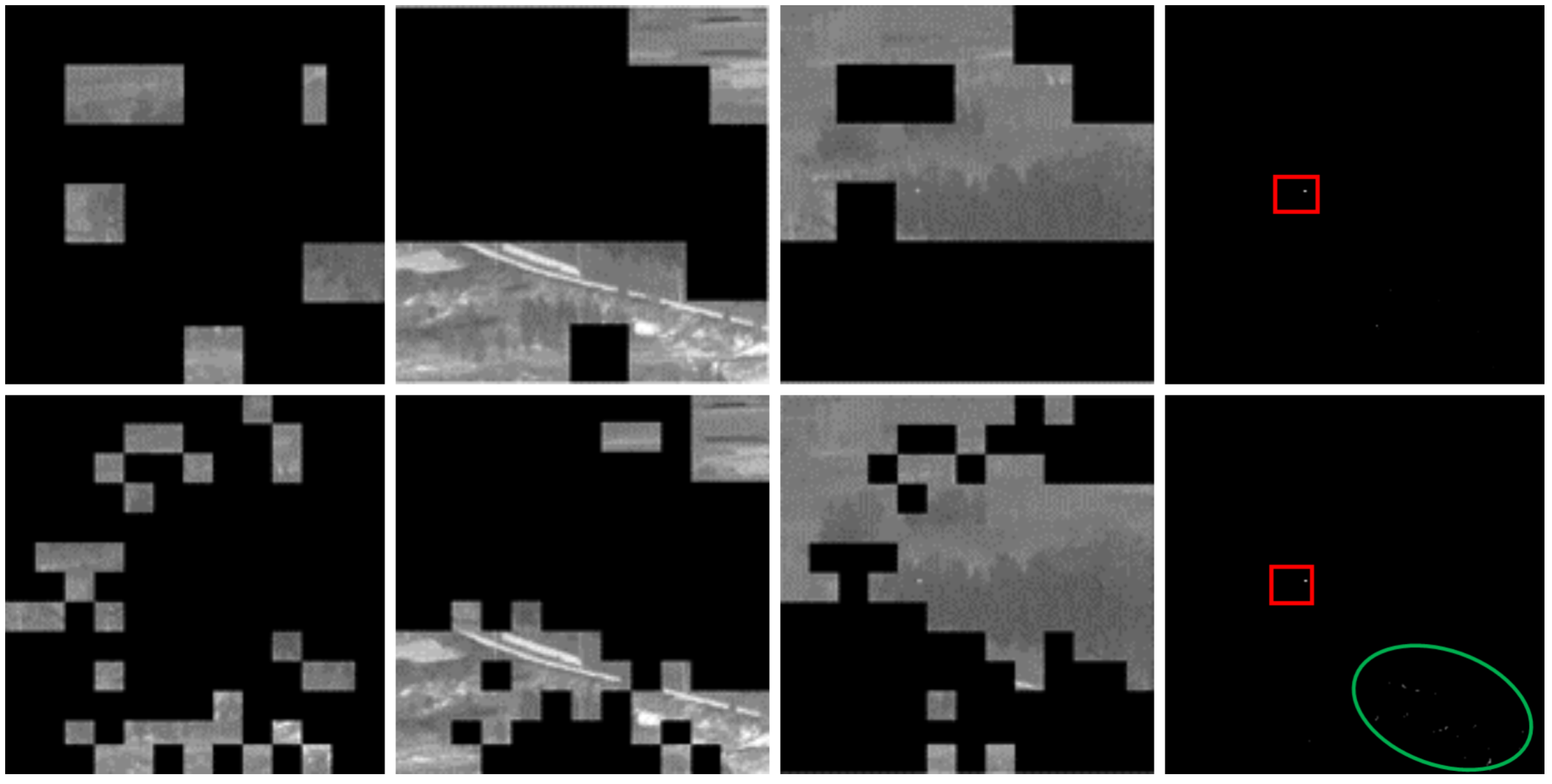
As shown in the first row of Figure 2, the size of the sliding window used in the first row is 40 × 40; the target image only contains the target, and the background residual of strong edges is completely removed. The size of the sliding window used in the second row is 20 × 20, and the background residual exists in the target image, which increases the likelihood of false alarms. In order to illustrate this problem, statistical analysis is carried out on two image sequences. The target size in the two image sequences is the same, meaning that the sliding window size to achieve optimal performance of the two sequences should be similar; however, the ROC curve in Figure 3 show that this is not the case. For the first sequence, the optimum is achieved when the sliding window is set to 50, while for the second sequence the effect is poor when the sliding window is set to 50; thus, it is obvious that the first sequence is more sensitive to the sliding window than the second one. The fundamental reason behind this result is that the grouping method is based on the probability of the block image belonging to a certain feature; thus, the size of the sliding window affects which group the block image is divided into. The method of using a fixed-size sliding window to intercept pixels does not consider the integrity of local features in the image, leading to a complete object being divided into several parts, which are divided into different groups. Therefore, a more reasonable segmentation method is needed to more accurately describe the characteristics of the block image in order to maintain the integrity of the local features of the image.
Superpixels are irregular regions composed of pixels with similar features. These small areas retain the relevant information of the local area; furthermore, because of the settings in the algorithm, the boundary information in the object is usually well preserved and is not destroyed. Therefore, superpixels are widely used in image preprocessing, object detection, image classification, and other fields. Among the available methods, Simple Linear Iterative Clustering (SLIC) [52] has the advantages of simplicity and efficiency, and has attracted the attention of many scholars. For an input image, the main idea of the SLIC algorithm is as follows: first, the image is divided into an S × S regular grid; in order to avoid the edge parts or noisy points in the image becoming the center of the current superpixel, the cluster center is taken as the minimum gradient position in its 3 × 3 neighborhood during each calculation, then different features are selected as the similarity measure. As shown in Figure 4, the similarity value is usually computed by searching in the neighborhood of 2S × 2S from the center of superpixel, and it is assigned to the nearest cluster center. Finally, after iteration, when the residual of the cluster center in the last iteration is less than the threshold, the iteration is stopped and the final superpixel segmentation result is obtained. Because infrared images do not have color information, the gray distance and spatial distance are selected as similarity measures in this paper. For a cluster center C i = l i x i y i , the Euclidean distance D between it and each pixel in its neighborhood is calculated as follows:
d c = l p l q 2
d s = x p x q 2 + y p y q 2
D = d c 2 + α d s S 2
where d c represents the grayscale distance, d s represents the spatial distance, and α is a constant.
As shown in Figure 4, irregular regions are obtained after superpixel segmentation, and the size of image blocks needs to be consistent during tensor calculation. Therefore, we take the maximum size of the region obtained by superpixel segmentation as the uniform size of the image block when constructing the tensor, and expand the region smaller than this size from the center to the periphery to fill with the original pixel. Thus, the construction of the tensor is completed.

3.2. Description of Features Exploiting the Structure Tensor

The structure tensor, in contrast to the gradient, enhances local structural characteristics by employing a smoothing procedure and assessing the coherence of the spatial orientations surrounding each pixel. Assuming that D represents the original image, we can calculate the conventional structure tensor with a linear configuration as described in Equation (5) [53,54]:
J = K ρ D σ D σ = K ρ I x 2 K ρ I x I y K ρ I x I y K ρ I y 2 = J 11 J 12 J 21 J 22
where K ρ represents a kernel function with a Gaussian distribution and variance ρ , while D σ denotes a Gaussian smoothing filter with variance σ applied to the original image. The gradients of D σ with respect to x and y , denoted as I x = D σ / x and I y = D σ / y , respectively, are obtained through a convolution operation. The gradient operator is represented by ∇, and the Kronecker Product is used. It should be noted that the structure tensor has dimensions of 2 × 2. The local image features can be enhanced by employing principal axis transformation in the structure tensor, thereby improving their discriminative power and facilitating more accurate analysis:   
J = S T Λ S = m λ m j m j m T
where S = j 1 , j 2 T and j 1 j 2 is the structure tensor J characteristic vector, while Λ = diag λ m is a diagonal matrix of eigenvalues. The computation of the structure tensor’s two eigenvalues is performed through
λ 1 , λ 2 = J 11 + J 22 ± J 22 J 11 2 + 4 J 12 2 .
The characteristics of the image can be represented by the top two eigenvalues of the structure tensor under various conditions involving λ 1 and λ 2 . First, λ 1 λ 2 0 , indicating a corner region. It can be observed that the partial derivative amplitude is similar in two vertical directions; however, there is a noticeable difference in their respective orientations. This discrepancy indicates a variation in the location of this performance, particularly towards the corner. Second, λ 1 λ 2 0 , indicating an edge region. This implies that the partial derivative at this particular position exhibits a minimal change in one direction, approaching zero, while displaying a substantial variation in the perpendicular direction. This pronounced dissimilarity signifies a distinct orientation, thereby indicating a high likelihood of the point being situated on an edge. Third, λ 1 λ 2 0 , indicating a flat region. This implies that the partial derivative at this particular position exhibits minimal variation in all directions, approaching zero. Consequently, the grayscale transition occurs gradually, indicating a high likelihood of the point being situated within a flat region.
Although both the RIPT model [30] and PSTNN model [32] utilize the structure tensor, they do not simultaneously incorporate all three types of feature points; instead, only one or two of them are utilized. In order to maximize the utilization of these three types of features, we have devised the following functions to depict the characteristics exhibited in infrared images:
ω a = 1 2 e λ 1 λ 2 + 0.003 1 e λ 1 λ 2 λ 1 + e λ 2 λ 2 λ 1 , ω b = e λ 1 λ 2 + 0.003 1
where ω b serves as a measure of the amplification factor indicating the difference between λ 1 and λ 2 . When ω a approaches infinity, this indicates that a pixel lies in an edge region and should be categorized as a line feature. Conversely, when ω a approximates 1, it can be regarded as a flat feature while considering other parts of the initial area as point features. Nevertheless, careful selection of suitable threshold values becomes crucial due to noise interference and potential over-amplification caused by ω b . The decision-making process for thresholds can be summarized accordingly:
class p = a 1 max ( P ) , class f = a 2 min ( P )
class p 1 = a 3 min ( Q ) , class f 1 = a 4 min ( Q )
where a 1 , a 2 , a 3 , and a 4 are fixed values, while P and Q denote the remaining elements obtained by removing infinity from sets ω a and ω b , respectively. By conducting an exploration to satisfy the aforementioned criteria
ω a ( x , y ) > Class p and ω b ( x , y ) Class p 1 , ( x , y ) point ω a ( x , y ) = and ω b ( x , y ) > Class p 1 , ( x , y ) line ω a ( x , y ) Class f and ω b ( x , y ) Class f 1 , ( x , y ) flat
the (x, y) coordinates represent the pixel position. The corner region contains point features, the edge region contains line features, and the flat region contains flat features.

3.3. The Cluster 4D-FCTN Model

3.3.1. Four-Dimensional Infrared Image Tensor Model

IR small target detection models based on low-rank and sparse decomposition generally assume the presence of target, noise, and background in the original image. This assumption allows for an approximate modeling of the image, as follows:
f D = f B + f T + f N
where f D , f B , f T , and f N represent the initial image, backdrop image, desired image, the noise image, respectively. The IPI model represents an optimal approach for maximizing the utilization of this characteristic, as illustrated below:
D = B + T + N
where T, B, N, and D represent the target, background, noise, and the original infrared image.
The presence of spatial correlation between adjacent pixel data in the image is disrupted by employing the “pulling vector” approach for each image block in the image block matrix method, leading to a decline in detection performance. Conversely, utilizing the “pulling vector” technique for each image patch within the image patch matrix method disrupts this spatial correlation and results in a decrease in detection performance. To enhance the model’s performance, we introduce a novel approach called image patch tensor (IPT). This method shares similarities with the IPI model, and is represented in Equation (14):
D = B + T + N
where D , B , T , N R m 1 m 2 m 3 stand for the original image tensor, the background tensor, the target tensor, and the noise tensor, respectively.
However, both methods exhibit limited effectiveness in complex infrared environments. Moreover, the computational complexity is further exacerbated by the need for restacking after tensor generation, hindering the efficiency of execution. In order to boost local correlation and retain temporal data, Wu [38] recently presented a novel 4D infrared tensor model that eliminates the need for restacking and enhances the tensor order, enabling effective extraction of spatial–temporal information through high-order decomposition-based optimization. Consequently, the proposed formulation of the 4D infrared tensor D 4 D can be expressed as follows:
D 4 D = B 4 D + T 4 D + N 4 D
where D 4 D , B 4 D , T 4 D , and N 4 D R M 1 × M 2 × M 3 × M 4 . Here, M 3 represents the number of consecutive frames in an image sequence, while M 1 and M 2 are patch sizes ( M 1 = M 2 ), Additionally, we define both the sliding step M s and window size M 1 to have equal values. Lastly, we use M 4 to indicate the total quantity of generated patches.
It is possible to place a constraint on D 4 D by taking advantage of the low-rank feature of the 4D background tensor [38]:
rank B 4 D r
where the complexity of the background is denoted by a positive constant r.
Usually, spatially sparse distributions characterize tiny infrared targets which occupy a limited area. Despite environmental fluctuations occurring rapidly, these targets only cover a small fraction of their trajectory zone over time. As a result, they maintain their sparsity even within temporal patch volumes. This property guarantees that the 4D target tensor T 4 D satisfies the following condition:
T 4 D α
where the value of α is determined by the characteristics and number of the targets. Subsequently, the low-ranking background and sparse target can be effectively separated through TRPCA modeling:
min B 4 D , T 4 D rank B 4 D + λ 1 T 4 D 0 s . t . D 4 D = B 4 D + T 4 D + N 4 D
where the weighting parameter λ 1 regulates the overall tradeoff between the target patch-tensor T 4 D and the background patch-tensor B 4 D .
However, the fourth dimension of the 4D tensor constructed by the algorithm does not fully maintain the spatial continuity and correlation of patches, that is, all patches are arranged into a row to form the fourth dimension, which destroys the spatial structure of the patches.

3.3.2. ISTD Based on C4D-FCTN

Based on the problems of the ordinary 4D tensor model, we propose a feasible classification and combination of 3D patch tensors to form several kinds of more relevant 4D tensors to solve such limitations.
In a complex background, strong edges sometimes only occupy a small portion of the image with distinct edge characteristics. However, more blocks may be required to adequately capture the low-rank property of the background in such cases. To address this issue, we propose modeling and grouping similar feature blocks that satisfy the low-rank property within their respective spaces. This approach aligns better with the low-ranking nature of the background and enables parallel computation through block grouping, thereby reducing computational time.
The infrared image features can be clustered into three groups based on the tensor feature description, which is the foundation for calculating the probability of belonging to each group within a block. The image patches exhibiting significant similarities are naturally grouped together. The probability of the i-th patch belonging to the three features can be computed as follows:
P i ( point , line , flat ) = k i ( piont , line , flat ) max k point , k line , k flat
where k i (point, line, flat) represents the number of pixels belonging to point features, line features, and flat features in the i-th image patch, while k point , k line , and k flat represent the number of pixels belonging to point features, line features, and flat features in all image patches.
After grouping the block images, we tested the low-rank property of tensors in each cluster and performed singular value decomposition on them. The results are presented in Figure 5, where (a) denotes the original image, (b) represents the singular value curve of the point feature cluster tensor, (c) shows the singular value curve of the line feature cluster tensor, and (d) displays the singular value curve of the flat feature cluster tensor. It is evident that different clusters possess their own intra-cluster low-rank properties; hence, the background can be modeled on this basis.
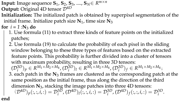
After the completion of the aforementioned clustering process, instead of stacking the spatial tensor patches in series, we rearrange the 3D patches with the same feature type into the same cluster to form the 4D tensor (that is, the four dimensions of the 4D tensor are the length of the sliding window, width of the sliding window, sequence index, and sliding window index within a cluster). Specifically, as described in Algorithm 1, the initialized patch is obtained by adaptively selecting the sliding window size through superpixel segmentation of the initial frame. Subsequently, the feature detection function in Formula (11) is used to extract three kinds of feature points on the initialized patch. The clustering criterion in Formula (19) is then applied to calculate the probability of each pixel in the sliding window belonging to these three types of features based on the extracted feature points. This probability is further divided into a cluster of tensors with maximum probability, resulting in three 3D tensors: D 3 D p , D 3 D l , and D 3 D f . Subsequently, each patch in the N 3 frames are classified as the corresponding patch at the same position as the initial frame, thereby stacking the image patches into three 4D tensors: D 4 D p , D 4 D l , and D 4 D f .
The stacking is performed in the order of the third-order coordinates of the frame index N 3 , and the patch index N 4 is used as the fourth-order axis. The patches with the same feature type in the third dimension patch of a 4D tensor are rearranged into the same cluster to form three 4D tensors. Using MATLAB, we start by utilizing sliding window techniques to produce N 1 localized patches from a single image (the starting frame) for the purpose of constructing sub-three-way tensors. Subsequently, we utilize the operator for multidimensional arrays to accomplish the stacking process of the 4D tensor.
Algorithm 1: The process of building the 4D infrared image tensor for clustering
Remotesensing 16 00034 i001
A recent investigation [51] has unveiled the efficacy of the FCTN-based TRPCA technique in handling high-dimensional data, providing an accurate estimation of tensor rank. In comparison to alternative tensor decompositions, FCTN decomposition demonstrates superior performance when addressing challenges related to tensor completion. This advantage arises from its inherent ability to flexibly capture correlations among different modes. In this study, we propose a novel Cluster 4D-FCTN model that employs a new FCTN nuclear norm as a convex surrogate for quantifying mode correlations within our 4D model. For an Nth-order tensor X R M 1 × M 2 × × I N , we formulate the FCTN nuclear norm as follows:
B 4 D 4 D F C T N = k = 1 L β k B k n 1 k ; n 2 k *
where the weighting factors β k satisfy the condition k = 1 L β k = 1 , which are all positive, n k is the k-th rearrangement of the vector [ 1 , 2 , , N ] , n 1 k = n 1 : N / 2 k , n 2 k = n N / 2 + 1 : N k , and L = C N N / 2 .
To ensure low rank within clusters while maintaining each cluster’s independence from the others and global sparsity of targets, our proposed Cluster 4D Fully-Connected Tensor Network model (C4D-FCTN) is
min B 4 D , T 4 D , N 4 D i = 1 3 ( B i 4 D 4 D F C T N + λ 1 T 4 D 1 + λ 2 N 4 D F 2
s . t . D 4 D = B 4 D + T 4 D + N 4 D .
Our proposed method effectively utilizes the low-rank characteristics of the background and the sparse properties of the target, with the positive penalty parameter λ 2 responsible for regulating noise and B i 4 D denoting the background tensor of cluster i.
min B 4 D , T 4 D , N 4 D k = 1 L k = 1 3 β k B k n 1 k : n 2 k i * + λ 1 T 4 D 1 + λ 2 N 4 D F 2 s . t . D 4 D = B 4 D + T 4 D + N 4 D E = T 4 D B k = B 4 D

3.4. Resolution of the Proposed Model

We have developed the Cluster 4D-FCTN model for representing IR images. Subsequently, an Alternating Direction Method of Multipliers (ADMM) approach is employed to effectively address the provided optimization problem as a resilient tensor recovery task. By introducing auxiliary variables, Equation (22) is reformulated as follows:
L B 4 D , T 4 D , N 4 D , E , B k , X k , U , V = k = 1 i = 1 N k 3 β k B k n 1 k : n 2 k i * + < X k , B k i B i 4 D > + ω k 2 B k i B i 4 D F 2 + λ 1 T 4 D 1 + λ 2 N 4 D F + < U , F > + σ 2 F F 2 + < V , E T 4 D > + γ 2 E T 4 D F 2
s . t . F = D 4 D B 4 D T 4 D N 4 D
where the variables ω k , σ , and γ represent penalty parameters and where X k , U , and V denote Lagrangian multipliers. According to the ADMM framework [55], B k , E , B 4 D , and T 4 D can be divided into two subsets, with the variables in each subset being updated alternately.
B k t + 1 , E t + 1 = arg min B k , E L i = 1 3 B i 4 D t , T 4 D t , E , B k , X k t , U t , V t
B 4 D t + 1 , T 4 D t + 1 = arg min B 4 D , T 4 D L i = 1 3 B i 4 D , T 4 D , S t + 1 , B k t + 1 , X k t , U t , V t
Next, we provide additional information regarding each individual subproblem.
(1) Update B k . The formulation of subproblem B k (where k = 1, 2, …, L) can be readily converted into an equivalent representation:
B k t + 1 = arg min B k α k i = 1 3 B i k n 1 k ; n 2 k * + < X k , B k B 4 D > + ω k 2 B k B 4 D F 2 = arg min B k α k i = 1 3 B i k n 1 k ; n 2 k k + ω k 2 B k n 1 k ; n 2 k B 4 D t X k t ω k n 1 k ; n 2 k F 2
and the given equation possesses a closed-form solution
B k n 1 k ; n 2 k t + 1 = U Σ β k / ω k V T
where B 4 D t X k t ω k n 1 k ; n 2 k = U Σ V T , Σ β k / ω k = diag max Σ r , r β k / ω k , 0 and Σ r , r is the rth singular value of Σ . B k t + 1 = Y B k t + 1 .
(2) Update E . The E -subproblem is
E t + 1 = arg min E λ E 1 + V t , E T 4 D t + γ 2 E T 4 D t F 2 = arg min E λ E 1 + σ 2 E T 4 D t + V t γ F 2 ,
which can be solved analytically using the following formula:
E t + 1 = soft λ / σ T 4 D t V t σ
where the operator soft λ / σ represents a soft shrinkage operation using a threshold value of  λ / σ .
(3) Update B 4 D t , T 4 D t . This subproblem ( B 4 D t , T 4 D t ) can be formulated as a problem of minimizing the sum of squared residuals:
B 4 D ( t + 1 ) , T 4 D ( t + 1 ) = arg min B i 4 D , T 4 D k = 1 L X k , B k B 4 D + ω k 2 B k B 4 D F 2 + < U , F > + γ 2 F F 2 + < V , E T 4 D > + σ 2 E T 4 D F 2 = arg min B 4 D , T 4 D k = 1 L ω k 2 B k t + 1 B 4 D + X k t ω k F 2 + σ 2 D 4 D ( t + 1 ) B 4 D T 4 D + U t σ F 2 + γ 2 E t + 1 T 4 D + V t σ F 2 .
and is acquired through
B 4 D ( t + 1 ) = σ K t ( σ + γ ) J t / σ 2 k = 1 L ω k + σ ( γ + σ )
and
T 4 D ( t + 1 ) = σ J t k = 1 L ω k + σ K t / σ 2 k = 1 L ω k + σ ( γ + σ ) ,
where J t = k = 1 L ω k B k 4 D ( t + 1 ) + X k t / ω k + σ D 4 D ( t + 1 ) + U t / σ and K t = σ ( D 4 D ( t + 1 ) + U t / σ ) + γ ( S t + 1 + V t / γ )
(4) Update the multipliers. The Lagrangian multipliers are modified using the following procedure:
X k t + 1 = X k t + α ω k B 4 D ( t + 1 ) B k t + 1 , k = 1 , 2 , , L U t + 1 = U t + α γ D 4 D B 4 D T 4 D V t + 1 = V t + α σ T 4 D E
where α is the step length.
The comprehensive procedural overview of the ADMM-based method for addressing the Cluster 4D-FCTN is presented in Algorithm 2.
Algorithm 2: Algorithm utilizing ADMM to solve the 4D-FCTN clustering problem.
  Input: Original infrared tensor D 4 D . parameter λ 1 , λ 2 , τ .
  Output: Background tensor B 4 D , target tensor T 4 D , and noise tensor N 4 D .
  Initialization: B 4 D = D 4 D , T 4 D , N 4 D , Multiplier of the Lagrangian function X k 0 ( k = 1 , 2 , , L ) , U , V , parameters ω k ( k = 1 , 2 , , L ) , γ .
  Update B k t + 1 by Formula (27);
  Update E t + 1 by Formula (29);
  Update B 4 D t + 1 and T 4 D t + 1 by Formulas (31) and (32);
  Update Lagrangian multiplies by Formula (33);
  Verify the condition of convergence: D 4 D B 4 D * T 4 D * N 4 D * F / D 4 D F < τ ;
  Should the convergence criteria not be satisfied, increment t by 1 and proceed to Step 1.
In summary, Figure 6 depicts the comprehensive process of identifying infrared targets through the proposed model. The subsequent stages are expounded upon as follows:
(1)
For a sequence of original images consisting of N frames, denoted as { S 1 , S 2 , , S N R m × n } , we create three Cluster 4D infrared image tensors D 4 D p , D 4 D l , and D 4 D f R N 1 × N 2 × N 3 × N 4 by organizing a sequence of N 3 frames in the correct temporal sequence using Algorithm 1, as described in Step 1 of Figure 6.
(2)
For the three obtained 4D tensors, each is decomposed into target 4D tensors T 4 D , background 4D tensors B 4 D , and noise 4D tensors N 4 D obtained through D 4 D by Cluster 4D-FCTN decomposition using Algorithm 2, as described in Step 2 of Figure 6.
(3)
We reconstruct the target images S 1 T , S 2 T , S 3 T , , S N 3 T R m × n from the 4D target tensor of the point feature ( T 4 D ) p , the 4D target tensor of the line feature ( T 4 D ) l , and the 4D target tensor of the flat feature ( T 4 D ) f using the reverse process outlined in Algorithm 1, as described in Step 3 of Figure 6.
Figure 6. Overall procedure of the Cluster 4D-FCTN model.
Remotesensing 16 00034 g006

3.5. Complexity Analysis

This section briefly touches upon the computational complexities associated with our proposed approach. To ensure uniformity, we denote the true dimensions of our 4D tensor as M 1 × M 2 × M 3 × M 4 . For Algorithm 2, we establish the constant x i as x i = i = 1 l M n i , y i as y i = i = l + 1 N M n i , l = N / 2 , and n as the rearrangement of vector ( 1 , 2 , , N ) . Thus, the update complexity of B k is O i = 1 L x i y i min x i , y i n , and the updating of B 4 D , T 4 D , and N 4 D are within the complexity of O i = 1 N M i . In addition, the computing complexity of X k , U , and V are O i = 1 N M i .

4. Experiment and Results

The effectiveness of the proposed the Cluster 4D-FCTN method is assessed in this section through a series of experiments. Initially, we present the experimental setup, which includes evaluation criteria, datasets, and baseline techniques. Subsequently, various crucial parameters are examined and the resilience of our model is evaluated. Additionally, a comparative analysis is conducted between our method and other competitive approaches. Lastly, a series of ablation studies demonstrates that techniques elevating the dimensionality to 4D and conducting clustering computations yield more favorable outcomes compared to analogous methods based on 3D data and 4D approaches without clustering. This section additionally encompasses a discussion on limitations and future directions.

4.1. Data and Experiment Settings

To provide a more objective assessment of the Cluster 4D-FCTN model’s performance and facilitate comparisons with other models, we performed trials on five different sets of images captured in diverse environments, as listed in Table 1. The dataset utilized in our research comprised infrared images, as suggested by Hui et al. [56]. Figure 7 exhibits representative images captured from these sequences, featuring expanded target regions showcased in the upper right-hand corner of every picture. Sequences 1 and 2 exhibit significant local contrast variations while featuring background consisting of trees and man-made structures, posing a moderate detection challenge. Sequence 3 presents low contrast levels and noticeable background radiation, making it particularly challenging to detect targets. In Sequence 4, several radiation sources emitting high-intensity levels in the surrounding environment can significantly increase false alarm rates. On the other hand, Sequence 5 is relatively straightforward; however, it encompasses a large target area that necessitates algorithms capable of preserving target integrity.

4.2. Evaluation Metrics and Baselines

In this study, a performance assessment of infrared target detection algorithms employing five prevalent metrics is presented. These measurements include the ROC curve for receiver operating characteristic, the SCRG, which represents the signal-to-clutter ratio gain, the LSNRG, which denotes the local signal-to-noise ratio gain, the BSF, indicating the background suppression factor, and CG, which represents the contrast gain:
SCRG = SCR out SCR in , BSF = σ out σ in
where SCR in and SCR out are the SCR values of the original image and the recovered target image. Similarly, the standard deviations between the original image and the reconstructed target image are represented by σ out and σ in . The ROC curves are depicted based on the false alarm ratio (Fa) and the probability of detection (Pd), as outlined below:
Fa = the quantity of identified false targets the total number of pixels throughout the entire image .
Pd = the quantity of detected true targets the aggregate count of authentic targets .
where Fa represents the abscissa and Pd denotes the ordinate.
In addition, we employ the LSNRG for evaluating the ability to enhance the target, quantified as follows:
LSNRG = LSNR out LSNR in
where LSNR out and LSNR in denote the respective LSNR values of the initial image and the modified image,
LSNR = P T P B
where P T and P B denote the highest pixel values of the surrounding area and the target, respectively. Lastly, we present the CG, which is expressed as follows:
CG = CON out CON in
where CON out and CON in represent the contrast of the initial and modified image, respectively, with CON defined as
CON = σ in σ out ,
where σ in and σ out have identical values to those in Equation (34).
In our comparative analysis, we incorporated six state-of-the-art ISTD methods as benchmarks. Specifically, these methods included a matrix-based IPI approach [29], a tensor-singleframe-based RIPT technique [30], a PSTNN algorithm [32], a tensor sequence-based ECASTT method [35], an MFSTPT model [36], and SRSTT, a sparse regularization-based twist tensor model [37]. The detailed parameter configurations are presented in Table 2.

4.3. Parameter Settings

The λ 1 parameter affects the resilience of different scenarios. A larger λ 1 is required to reduce false alarms in the target image, while a smaller λ 1 is needed to enhance the rate of identification for the target image. To evaluate the influence of λ 1 on the detection accuracy, we conducted tests and plotted ROC curves for different values of λ 1 , which are presented in the second column of Figure 8. The results indicate that there is an initial improvement in detection ability as λ 1 increases, and that this trend reverses beyond a certain threshold. Thus, we imposed a constraint on the upper limit of λ 1 when it reached 2. We correlated it with the number of image patches to establish the following:
λ 1 = min L N p N p l N p N p p , 2
where N p is the total number of patches, N p l is the number of patches of line type, and N p p is the number of patches of point type.
According to the findings presented in the third column of Figure 8, the ROC curves achieve their peak initial value when L is set at 0.6. Consequently, we opted for this value for L. The empirical setting for λ 2 was established as 100, following [35]. It has been documented that penalty factors escalate with the number of iterations. Consequently, we decide to set ω k * as σ ω k and γ * as σ γ , where ρ represents a numerical constant and its value corresponds to σ = 1.2. Furthermore, in our experiments both ω k and γ were assigned a value of 1 × 10 4 .

4.3.1. Patch Size N 1

Traditional algorithms may need to test the size of the sliding window and the sliding step in order to choose an appropriate size. In order to enhance the robustness of the sliding window size and sliding step length, in this paper we propose an algorithm that draws inspiration from superpixel segmentation. This algorithm uses a specific sliding step size, and only requires initialization of the mesh size S. As depicted in the first column of Figure 8, images were individually tested with grid initialization sizes ranging from 5–50 using a uniform selection of ten parameters. It is evident from the ROC curve that this algorithm is not sensitive to variations in grid initialization size, even when scaling the horizontal coordinate down to the 105 differences observed among the ROC curves under different initialization sizes. This finding confirms that utilizing superpixel segmentation enhances the algorithm’s resilience towards changes in window size.

4.3.2. Temporal Size N 3

The temporal dimension N 3 plays a crucial role in the construction and optimization of 4D tensors. Insufficient frames can lead to the loss of low-rank features and inefficient utilization of time domain data, while an excessive number of frames may result in increased time complexity, redundancy, repetition, and diminished time sparsity. To address this issue, we conducted experiments with varying values of L (10, 20, 30, and 40). The results are presented in the final column of Figure 8. Our findings indicate that G4D−FCTN performs optimally when N 3 is set to 20. Consequently, we chose N 3 as 20 for subsequent experiments.

4.4. Robustness of Scene Perception in Real-World and Synthetic Noisy Environments

In this section, we assess the robustness of the Cluster 4D-FCTN model across diverse environments and varying noise intensities.

4.4.1. Robustness in Diverse Environmental Conditions

The first row (a)–(f) of Figure 9 displays four infrared (IR) images depicting different scenes and sizes: 320 × 240, 256 × 172, 252 × 213, 256 × 256, 320 × 240, and 320 × 240, respectively. Figure 9a,b represent sky scenes, Figure 9c,d depict land scenes, and Figure 9e,f show ocean scenes. The second row (g)–(l) corresponds to the test results for these images; red boxes have been used to highlight all objects. The clustered 4D-FCTN model accurately detects small targets across various scenes while effectively suppressing background interference. This observation underscores the versatility of this model in adapting to diverse scenarios and datasets of different sizes.

4.4.2. Robustness against Noise

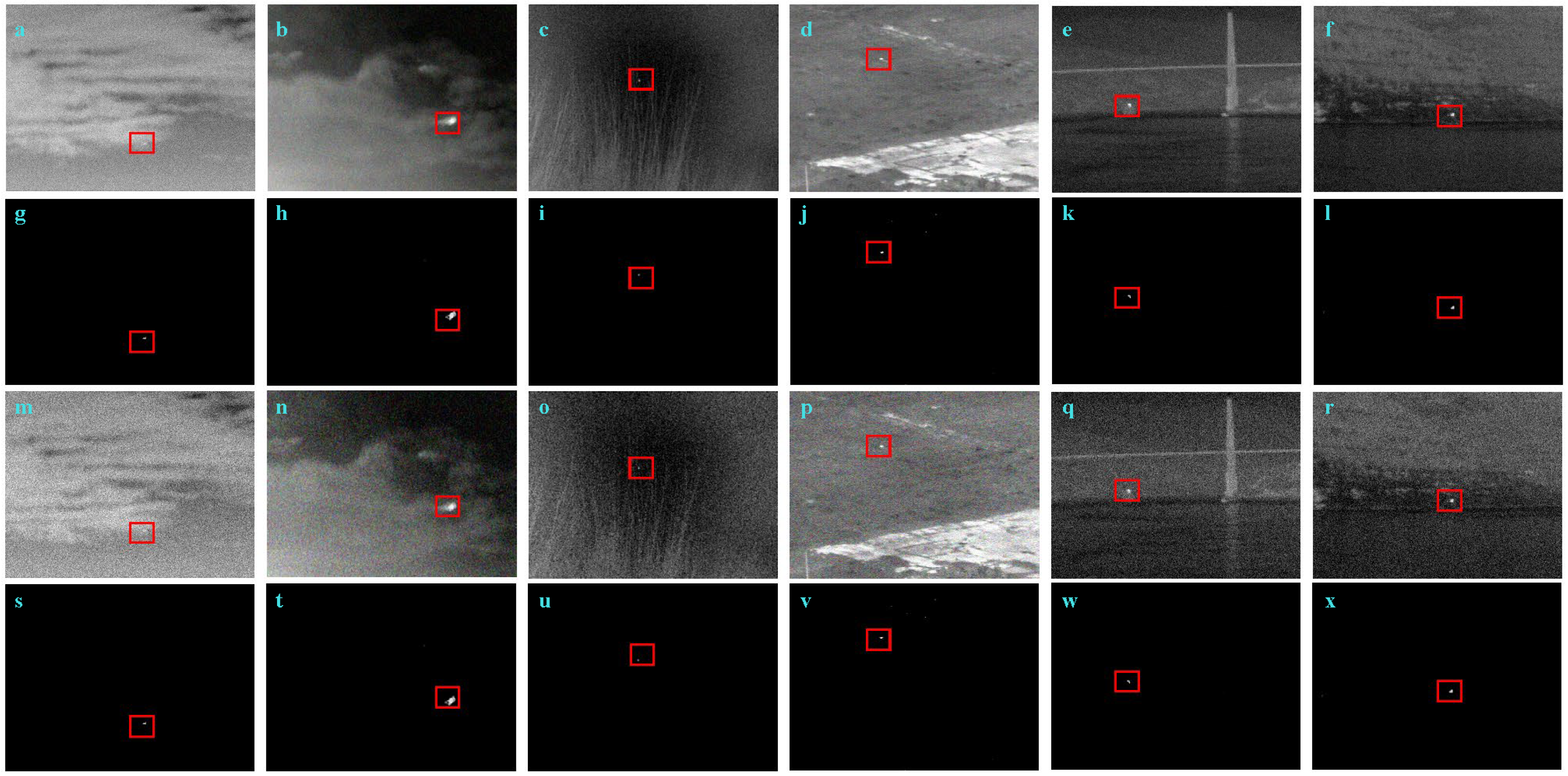
The application may result in noise presence within the acquired IR images, thereby necessitating the implementation of a test to evaluate the model’s ability to cope with such noise. To address this, we extracted six images from Figure 9 and injected Gaussian white noise with standard deviations of 10 and 20. This led to the generation of the corresponding noise maps presented in the first and third rows of Figure 10a–f. The second and fourth rows of Figure 10g–l display the recovered target images, which were obtained by applying the Cluster 4D-FCTN model to these noise maps. It is evident that the introduction of noise significantly exacerbates image blurriness, making it increasingly challenging to discern target features. Nonetheless, in spite of these obstacles, our Cluster 4D-FCTN model demonstrates robust detection capabilities while maintaining overall stability throughout various robustness tests conducted on single-frame images alone. Moreover, the employment of image sequences yields even more accurate detection results, as demonstrated by these experiments. Consequently, it can be concluded that the Cluster 4D-FCTN algorithm is able to effectively process single-frame images.

4.5. Comparison with Other Typical Methods

4.5.1. Visual Comparison

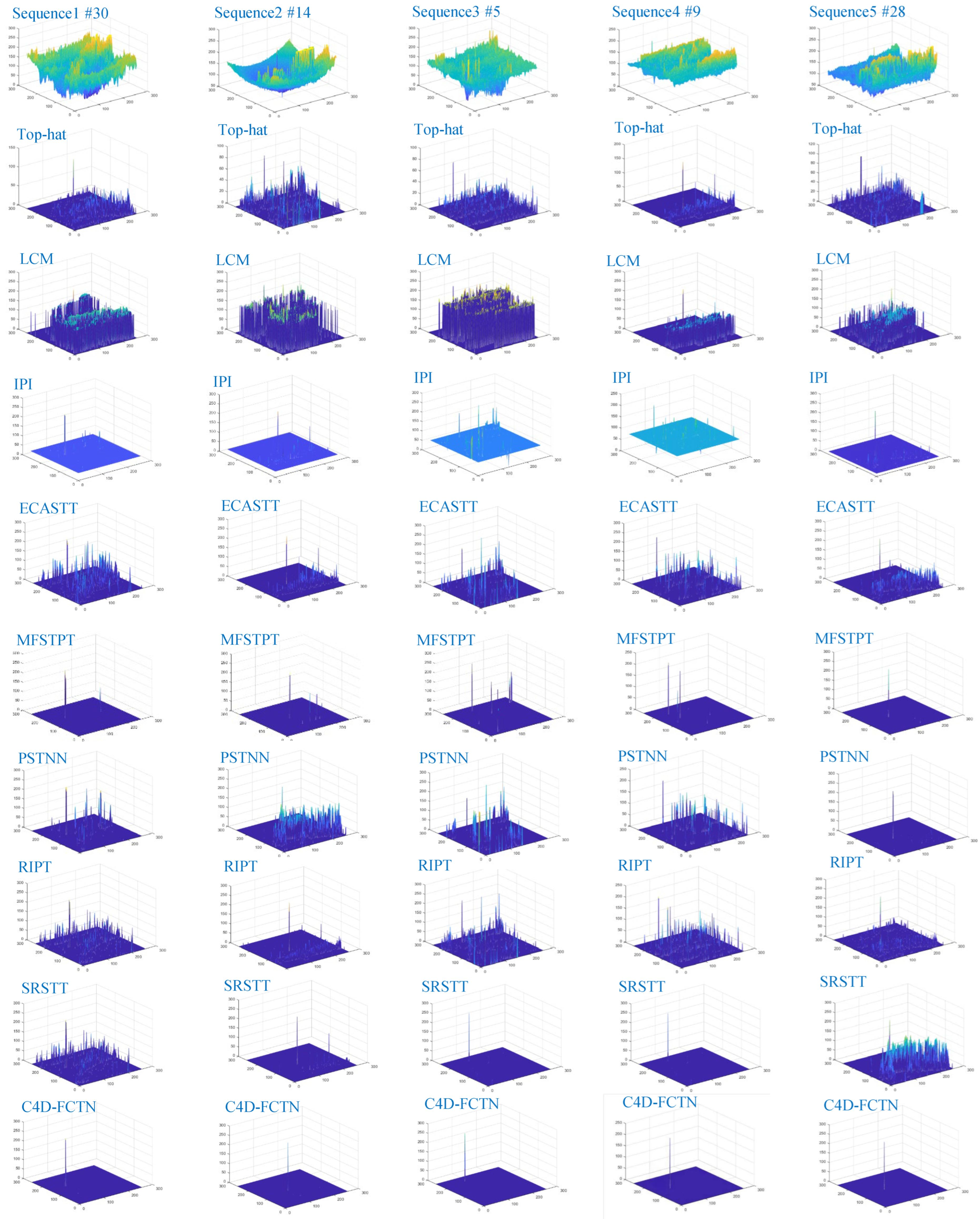
To provide a more objective performance evaluation of the Cluster 4D-FCTN model, we conducted tests employing various comparative algorithms on five distinct sequences of infrared images. Figure 11 displays the outcome images via three-dimensional surfaces.Additionally, the results for Sequences 1–5, which were not subjected to threshold segmentation, are presented in Figure 12. In the upper right corner, a magnified view (scaled by a factor of 2) accentuates the target zone, which is represented by a purple rectangle. Moreover, instances of failed detection are indicated by a dotted purple box. The IPI model demonstrates effectiveness in detecting targets across various sequences while maintaining their shapes; however, it encounters challenges with non-smooth backgrounds, resulting in images with pronounced edge residuals. The reason of this problem is that the nuclear norm is not accurate enough to constrain the strong edge background; treating all singular values equally leads to uniform shrinking, thereby compromising crucial details of these backgrounds. Consequently, strong edges are incorporated into the detected target images. In comparison to matrix-based methods, the RIPT and PSTNN tensor-based models exhibit superior ability to suppress complex backgrounds; however, they struggle with accurately reconstructing target shapes, especially when faced with scenarios such as Sequences 1–5, which contain numerous sparse objects within the backgrounds. Notably, neither PSTNN nor RIPT could detect any targets in Sequence 4. Sequence-based methods exhibit superior ability to suppress the background in intricate environments compared to single-frame approaches. ECASTT, MFSTPT, and SRSTT exhibit better preservation of the target’s edge shape. As observed in Sequences 1–3 and Sequence 4, the algorithms demonstrate accurate target detection. However, because of the relatively expansive size of the compact objectives in this series, the detected results partially suppress or magnify the targets. Moreover, MFSTPT and SRSTT fail to detect the target in Sequence 4. Our model and the IPI model exhibit the highest level of target shape retention integrity. Detecting artificial road structures in Sequences 1, 4, and 5 presents a challenge, in particular the presence of high-brightness background radiation in Sequence 2, which results in several methods retaining these backgrounds in their detection results. Among Sequences 1–5, only the Cluster 4D-FCTN model effectively suppresses clutter and noise across all frames. Sequence 4 poses the greatest difficulty, involving a small target with low contrast; the RIPT, PSTNN, and MFSTPT methods fail to detect the target, while the IPI and ECASTT methods retain significant noise areas. In contrast, our model effectively eliminates radiation sources with high-intensity background while striving to preserve the target’s integrity. In general, our model exhibits exceptional performance in detecting targets and suppressing background in all five sequences.

4.5.2. Qualitative Analysis

We conducted a quantitative assessment of the detection outcomes of the aforementioned methods across five sets of sequences utilizing the average values of SCRG, BSF, LSNRG, and CG calculated for each sequence. The resulting metric values are presented in Table 3, with the maximum value for each metric on each sequence highlighted in bold. It should be emphasized that if a single frame exhibits an Inf test value, this can result in an Inf average value for the entire sequence, encompassing the detection impact of other frames. Consequently, when calculating SCRG and BSF, we only consider them as Inf if the algorithm exhibits Inf values throughout the entire sequence; otherwise, we compute only the average of non-Inf values. Furthermore, Sequence 4 does not have targets detected by the PSTNN, RIPT, SRSTT, and MFSTPT methods; hence, they are excluded from the calculations. By definition, BSF evaluates the effectiveness of an algorithm in suppressing background across the entire image, while SCRG and CG assess its ability to enhance target presence and suppress background within local regions. Notably, the Cluster 4D-FCTN model demonstrates remarkably high BSF and SCRG values across all test sequences, indicating its exceptional capability to effectively remove background structures both locally and globally. Compared to its remarkable capacity for background suppression, our Cluster 4D-FCTN model demonstrates slightly inferior performance in target enhancement. The SRSTT model exhibits impressive outcomes in CG, particularly for Sequences 3–4. Nevertheless, when considering all algorithms across time, the Cluster 4D-FCTN model surpasses others in terms of overall evaluation based on the CG and LSNRG metrics. By integrating these three evaluation metrics, it becomes evident that the proposed Cluster 4D-FCTN model achieves superior outcomes by effectively suppressing background and enhancing targets, particularly in terms of background suppression.
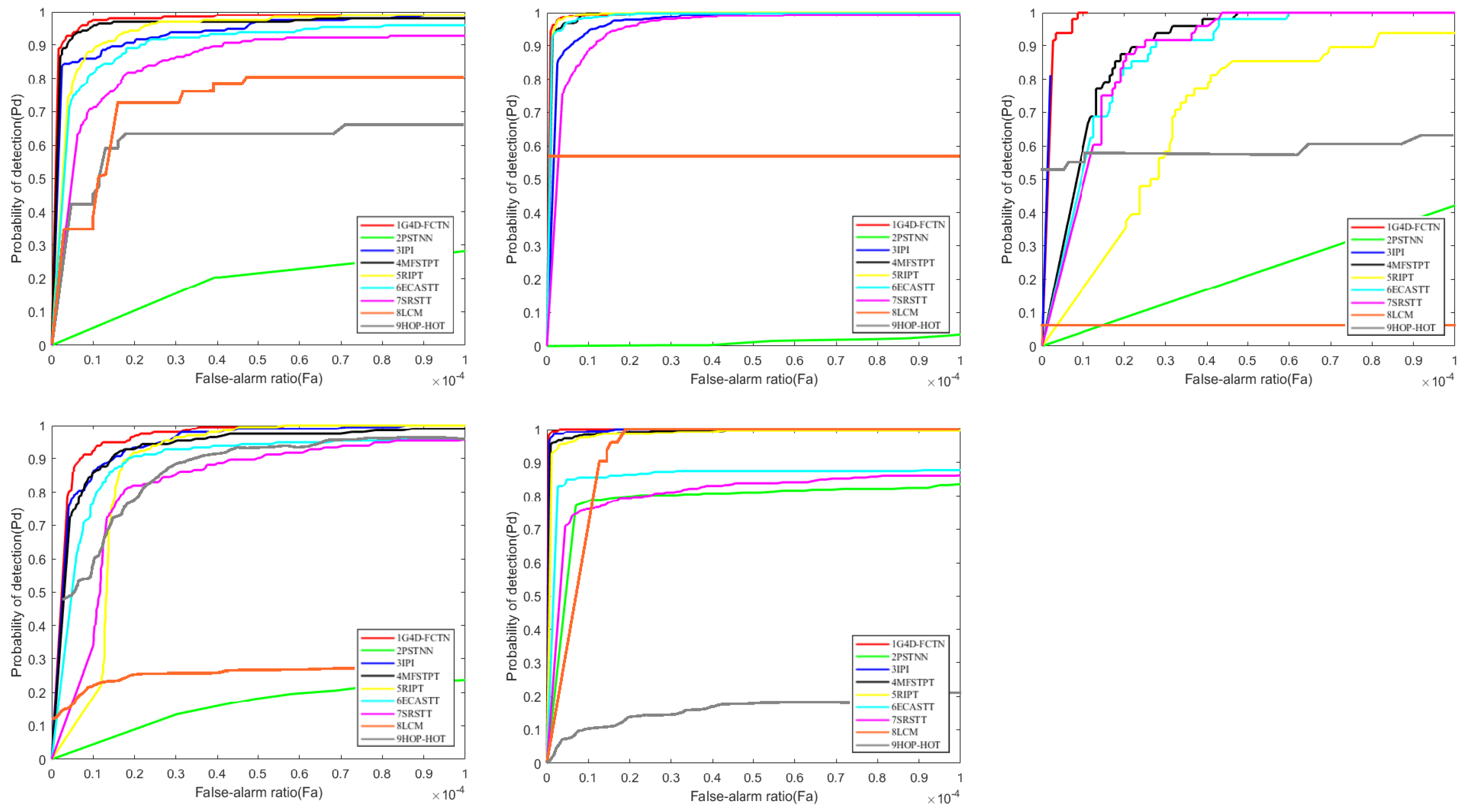
The performance evaluation of our algorithm in complex and noisy scenarios is illustrated by the five representative ROC curves shown in Figure 13, corresponding to Sequence 1 to 5. Our C4D-FCTN method consistently produces stable results even under challenging scenes, positioning itself relatively close to the top left corner, particularly evident in Sequence.4 and Sequence.5 where the presence of target-like objects may result in high false positive rates. Notably, single-frame methods such as RIPT and PSTNN fail when dealing with dark and small targets. In contrast, multi-frame methods outperform their single-frame counterparts across all sequences (Sequence.1–Sequence.5), highlighting the significance of temporal information for background noise suppression and object detection within sequence-based approaches. Nevertheless, some multi-frame methods like SRSTT and MFSTPT exhibit detection failures due to suboptimal utilization of time domain information, further emphasizing the effectiveness of our four-dimensional clustering tensor construction approach.
Figure 12 illustrates the assessment of various algorithms in intricate and turbulent surroundings (Sequences 1 through 5), with all of them exhibiting acceptable performance in simple scenarios. Our method consistently generates stable results in demanding situations, positioning itself proximate to the uppermost left corner, particularly in Sequences 4 and 5 in locations with objects resembling the target that might elevate false positive rates. Certain single-frame techniques, such as RIPT and PSTNN, manifest commendable detection outcomes on Sequences 1 and 2. Nonetheless, when confronting dim and small targets, strategies based on multiple frames surpass their single-frame counterparts on Sequence 3 to 5, precisely where our proposed technique outperforms them. This finding suggests that incorporating temporal information bolsters sequence-based methods in reducing background noise and augmenting target detection capabilities.

4.5.3. Comparison of Time Required for Computation

The runtime (per frame) of the seven algorithms across the five sequences is presented in Table 4. PSTNN emerges as the most proficient tensor-based method. Our approach exhibits a reduced computational time in the spatial–temporal tensor-domain.

4.6. Ablation Study

To demonstrate the efficacy and value of our dimensionality expansion and clustering strategies, we conducted an ablation study to evaluate the contributions of the Cluster 4D-FCTN model. We compared it to two other approaches: a spatial–temporal tensor construction-based 3D model (3DST-TCTN) akin to [57], and a model constructed by spatial–temporal tensor without clustering (4D-FCTN). The experiments were carried out on Sequences 1 to 5 with individually optimized parameter settings. As illustrated in Figure 14, the detection performance of Cluster 4D-FCTN surpasses both comparative methods in terms of ROC performance. Moreover, although 4D-FCTN achieves notable results across most datasets, the overall performance of Cluster 4D-FCTN outperforms both it and the 3D-based spatial–temporal tensor models. In conclusion, the integration of four-dimensional tensors provides enhanced detection capability in four-dimensional fields; however, our cluster four-dimensional tensor model demonstrates superior handling of ISTD tasks. Therefore, this experiment provides compelling evidence indicating that the employment of clustering calculations on four-dimensional data is both practical and highly effective.

5. Discussion

Infrared detection systems exhibit superior stealth capabilities and robust anti-jamming resistance, making them extensively applicable in both the military and civilian sectors. Infrared dim and small target detection constitutes a crucial component of these detection systems, and has emerged as a focal point of current research.
Considering that the background of infrared images has nonlocal autocorrelation and that the target occupies only a small number of pixels, scholars have proposed the application of low-rank sparse decomposition to the field of infrared small target detection. In this approach, the low rank of the background and the sparsity of the target are used to transform the target detection problem into a mathematical optimization problem to restore low-rank components and sparse components. This can satisfy the global prior of a low-rank sum target that is sparse in both simple and complex backgrounds. In recent years, a method of fusing local prior and temporal information to construct a low-rank sparse decomposition model that can effectively suppress false alarms has been developed. This method based on low-rank sparse decomposition is more suitable for complex and changeable scenes, and has better detection performance than other methods.
Although infrared dim and small target detection algorithms based on low-rank sparse decomposition have achieved a series of promising research results, there are several challenges that demand further study, mainly reflected in the following four aspects:
  • The method based on low-rank sparse decomposition involves many parameters, such as the size of the sliding window, the moving step of the sliding window, the weight coefficient in the objective function, and more. These parameters have an important impact on the performance of the algorithm.
  • At present, the construction of the tensor is relatively simple, generally using the sliding window to traverse the original infrared image or multi-frame sequence images to construct the tensor directly, which involves a large amount of redundant information that has nothing to do with the target.
  • The background tensor rank approximation is not accurate.
  • When utilizing time-domain information, existing algorithms based on low-rank sparse decomposition mainly fuse the time domain information into the image matrix or tensor data, and use multi-frame images instead of the original single-frame images to construct new data. However, the sequence information between the frames is not fully mined.

6. Conclusions

To address the issues related to sensitivity of sliding window size, inadequate utilization of time series data, and imprecise approximation of tensor rank in current methods for detecting infrared dim and small targets, this study introduces a novel approach based on superpixel segmentation and statistical clustering to construct a four-dimensional tensor model. Our model diverges from existing approaches that rely solely on information within the spatial domain at either a local or global level. Instead, our method utilizes both temporal and spatial information, and uses their correlation to construct a new model. By organizing 3D patches with the same feature type into the same group, we effectively exploit temporal characteristics; moreover, we connect local patches in sequential order to further capitalize on these temporal properties.
In addition, we propose a new tensor decomposition, called the Fully Connected Tensor Network (FCTN) decomposition, which facilitates the decomposition of an nth-order tensor into a sequence of low-dimensional nth-order factors. It breaks through the limitation that the exclusive role of TT and TR decomposition lies in the disclosure of the operation limited to two consecutive factors rather than the connection between any two factors, resulting in limited ability to measure the correlation. These issues are effectively resolved by leveraging the ADMM framework. In this paper, we extensively evaluate our methods on several datasets containing infrared sequences, employing five cutting-edge algorithms. Our results showcase superior detection accuracy and robustness in diverse scenarios compared to existing approaches. Moreover, a series of ablation studies demonstrate that the proposed techniques elevating the dimensionality to 4D and conducting clustering computations yield more favorable outcomes compared to analogous methods based on 3D data and 4D approaches without clustering. Finally, the Section 5 encompasses a discussion on limitations and future directions. Notably, the algorithm occasionally detects target-like items in fast-moving complex environments due to the absence of constraints on prior information regarding the target. Therefore, our future work aims to incorporate the prior knowledge of objects contained in the spatiotemporal features in order to facilitate object detection and mitigate false positives.

Author Contributions

W.W. was responsible for the conception and design of the experiments. W.W. conducted the experiments and drafted the manuscript. T.M. critically reviewed the manuscript and made revisions. M.L. provided guidance and edited the manuscript. H.Z. contributed computational resources and revised the manuscript. All authors have read and agreed to the published version of the manuscript.

Funding

This research received no external funding.

Data Availability Statement

Bingwei Hui et al., “A dataset for infrared image dim-small aircraft target detection and tracking under ground/air background”. Science Data Bank, 28 October 2019. Available Online: https://doi.org/10.11922/sciencedb.902 (accessed on 2 December 2022).

Conflicts of Interest

The authors declare no conflict of interest.

References

  1. Zhou, F.; Wu, Y.; Dai, Y.; Wang, P.; Ni, K. Graph-regularized laplace approximation for detecting small infrared target against complex backgrounds. IEEE Access 2019, 7, 85354–85371. [Google Scholar] [CrossRef]
  2. Ren, X.; Wang, J.; Ma, T.; Zhu, X.; Bai, K.; Wang, J. Review on infrared dim and small target detection technology. J. Zhengzhou Univ. (Nat. Sci. Ed.) 2020, 52, 1–21. [Google Scholar]
  3. Bai, X.; Bi, Y. Derivative entropy-based contrast measure for infrared small-target detection. IEEE Trans. Geosci. Remote Sens. 2018, 56, 2452–2466. [Google Scholar] [CrossRef]
  4. Li, J.; Zhang, P.; Wang, X.; Huang, S. Infrared small-target detection algorithms: A survey. J. Image Graph. 2020, 25, 1739–1753. [Google Scholar]
  5. Jinhui, H.; Yantao, W.; Zhenming, P.; Qian, Z.; Yaohong, C.; Yao, Q.; Nan, L. Infrared dim and small target detection: A review. Infrared Laser Eng. 2022, 51, 20210393-1. [Google Scholar]
  6. Liu, C.; Wang, H. Research on infrared dim and small target detection algorithm based on low-rank tensor recovery. J. Syst. Eng. Electron. 2023, 34, 861–872. [Google Scholar]
  7. Yang, W.P.; Shen, Z.K. Small target detection and preprocessing technology in infrared image sequences. Infrared Laser Eng. 1998, 27, 23–28. [Google Scholar]
  8. Deshpande, S.D.; Er, M.H.; Venkateswarlu, R.; Chan, P. Max-mean and max-median filters for detection of small targets. In Signal and Data Processing of Small Targets 1999 Denver, CO, United States; SPIE: Bellingham, DC, USA, 1999; Volume 3809, pp. 74–83. [Google Scholar]
  9. Yu, N.; Wu, C.Y.; Tang, X.Y.; Li, F.M. Adaptive background perception algorithm for infrared target detection. Acta Electonica Sin. 2005, 33, 200. [Google Scholar]
  10. Liu, Y.; Tang, X.; Li, Z. A new top hat local contrast based algorithm for infrared small target detection. Infrared Technol. 2015, 37, 544–552. [Google Scholar]
  11. Bi, Y.; Chen, J.; Sun, H.; Bai, X. Fast detection of distant, infrared targets in a single image using multiorder directional derivatives. IEEE Trans. Aerosp. Electron. Syst. 2019, 56, 2422–2436. [Google Scholar] [CrossRef]
  12. Lu, R.; Yang, X.; Li, W.; Fan, J.; Li, D.; Jing, X. Robust infrared small target detection via multidirectional derivative-based weighted contrast measure. IEEE Geosci. Remote. Sens. Lett. 2020, 19, 7000105. [Google Scholar] [CrossRef]
  13. Dong, L.; Wang, B.; Zhao, M.; Xu, W. Robust infrared maritime target detection based on visual attention and spatiotemporal filtering. IEEE Trans. Geosci. Remote Sens. 2017, 55, 3037–3050. [Google Scholar] [CrossRef]
  14. Han, J.; Liu, C.; Liu, Y.; Luo, Z.; Zhang, X.; Niu, Q. Infrared small target detection utilizing the enhanced closest-mean background estimation. IEEE J. Sel. Top. Appl. Earth Obs. Remote Sens. 2020, 14, 645–662. [Google Scholar] [CrossRef]
  15. Yang, L.; Yang, J.; Yang, K. Adaptive detection for infrared small target under sea-sky complex background. Electron. Lett. 2004, 40, 1. [Google Scholar] [CrossRef]
  16. Qi, S.; Ma, J.; Li, H.; Zhang, S.; Tian, J. Infrared small target enhancement via phase spectrum of quaternion Fourier transform. Infrared Phys. Technol. 2014, 62, 50–58. [Google Scholar] [CrossRef]
  17. Sheng, Z.; Jian, L.; Jinwen, T. Research of SVM-based infrared small object segmentation and clustering method. Signal Process. 2005, 21, 515–519. [Google Scholar]
  18. Dong, X.; Huang, X.; Zheng, Y.; Bai, S.; Xu, W. A novel infrared small moving target detection method based on tracking interest points under complicated background. Infrared Phys. Technol. 2014, 65, 36–42. [Google Scholar] [CrossRef]
  19. Zhao, J.; Tang, Z.; Yang, J.; Liu, E. Infrared small target detection using sparse representation. J. Syst. Eng. Electron. 2011, 22, 897–904. [Google Scholar] [CrossRef]
  20. Liu, D.; Li, Z.; Liu, B.; Chen, W.; Liu, T.; Cao, L. Infrared small target detection in heavy sky scene clutter based on sparse representation. Infrared Phys. Technol. 2017, 85, 13–31. [Google Scholar] [CrossRef]
  21. Xu, K.; Hu, W.; Zhou, W.; Zheng, H. Target detection based on the artificial neural network technology. In Proceedings of the 2006 9th International Conference on Control, Automation, Robotics and Vision, Orlando, FL, USA, 15–19 May 2006; pp. 1–5. [Google Scholar]
  22. Ma, Q.; Zhu, B.; Cheng, Z.; Zhang, Y. Detection and recognition method of fast low-altitude unmanned aerial vehicle based on dual channel. Acta Opt. Sin. 2019, 39, 105–115. [Google Scholar]
  23. Hou, Q.; Wang, Z.; Tan, F.; Zhao, Y.; Zheng, H.; Zhang, W. RISTDnet: Robust infrared small target detection network. IEEE Geosci. Remote Sens. Lett. 2021, 19, 1–5. [Google Scholar] [CrossRef]
  24. Dai, Y.; Wu, Y.; Zhou, F.; Barnard, K. Attentional local contrast networks for infrared small target detection. IEEE Trans. Geosci. Remote Sens. 2021, 59, 9813–9824. [Google Scholar] [CrossRef]
  25. Zhang, X.; Ren, K.; Wan, M.; Gu, G. Infrared small target tracking based on sample constrained particle filtering and sparse representation. Infrared Phys. Technol. 2017, 87, 72–82. [Google Scholar]
  26. Fan, X.; Li, J.; Chen, H.; Min, L.; Li, F. Dim and small target detection based on improved hessian matrix and F-Norm collaborative filtering. Remote Sens. 2022, 14, 4490. [Google Scholar] [CrossRef]
  27. Liu, D.; Li, Z.; Wang, X.; Zhang, J. Moving target detection by nonlinear adaptive filtering on temporal profiles in infrared image sequences. Infrared Phys. Technol. 2015, 73, 41–48. [Google Scholar] [CrossRef]
  28. Fan, X.; Li, J.; Min, L.; Feng, L.; Yu, L.; Xu, Z. Dim and Small Target Detection Based on Energy Sensing of Local Multi-Directional Gradient Information. Remote Sens. 2023, 15, 3267. [Google Scholar] [CrossRef]
  29. Gao, C.; Meng, D.; Yang, Y.; Wang, Y.; Zhou, X.; Hauptmann, A.G. Infrared patch-image model for small target detection in a single image. IEEE Trans. Image Process. 2013, 22, 4996–5009. [Google Scholar] [CrossRef] [PubMed]
  30. Dai, Y.; Wu, Y. Reweighted infrared patch-tensor model with both nonlocal and local priors for single-frame small target detection. IEEE J. Sel. Top. Appl. Earth Obs. Remote Sens. 2017, 10, 3752–3767. [Google Scholar] [CrossRef]
  31. Wang, X.; Peng, Z.; Kong, D.; Zhang, P.; He, Y. Infrared dim target detection based on total variation regularization and principal component pursuit. Image Vis. Comput. 2017, 63, 1–9. [Google Scholar] [CrossRef]
  32. Zhang, L.; Peng, Z. Infrared small target detection based on partial sum of the tensor nuclear norm. Remote Sens. 2019, 11, 382. [Google Scholar] [CrossRef]
  33. Cao, Z.; Kong, X.; Zhu, Q.; Cao, S.; Peng, Z. Infrared dim target detection via mode-k1k2 extension tensor tubal rank under complex ocean environment. ISPRS J. Photogramm. Remote Sens. 2021, 181, 167–190. [Google Scholar] [CrossRef]
  34. Kong, X.; Yang, C.; Cao, S.; Li, C.; Peng, Z. Infrared small target detection via nonconvex tensor fibered rank approximation. IEEE Trans. Geosci. Remote Sens. 2021, 60, 1–21. [Google Scholar] [CrossRef]
  35. Zhang, P.; Zhang, L.; Wang, X.; Shen, F.; Pu, T.; Fei, C. Edge and corner awareness-based spatial–temporal tensor model for infrared small-target detection. IEEE Trans. Geosci. Remote Sens. 2020, 59, 10708–10724. [Google Scholar] [CrossRef]
  36. Hu, Y.; Ma, Y.; Pan, Z.; Liu, Y. Infrared dim and small target detection from complex scenes via multi-frame spatial–temporal patch-tensor model. Remote Sens. 2022, 14, 2234. [Google Scholar] [CrossRef]
  37. Li, J.; Zhang, P.; Zhang, L.; Zhang, Z. Sparse Regularization-Based Spatial–Temporal Twist Tensor Model for Infrared Small Target Detection. IEEE Trans. Geosci. Remote Sens. 2023, 61, 1–17. [Google Scholar] [CrossRef]
  38. Wu, F.; Yu, H.; Liu, A.; Luo, J.; Peng, Z. Infrared Small Target Detection Using Spatio-Temporal 4D Tensor Train and Ring Unfolding. IEEE Trans. Geosci. Remote Sens. 2023. [Google Scholar]
  39. Sun, Y.; Yang, J.; Long, Y.; An, W. Infrared small target detection via spatial–temporal total variation regularization and weighted tensor nuclear norm. IEEE Access 2019, 7, 56667–56682. [Google Scholar] [CrossRef]
  40. Liu, H.K.; Zhang, L.; Huang, H. Small target detection in infrared videos based on spatio-temporal tensor model. IEEE Trans. Geosci. Remote Sens. 2020, 58, 8689–8700. [Google Scholar] [CrossRef]
  41. Liu, Y.Y.; Zhao, X.L.; Song, G.J.; Zheng, Y.B.; Huang, T.Z. Fully-connected tensor network decomposition for robust tensor completion problem. arXiv 2021, arXiv:2110.08754. [Google Scholar] [CrossRef]
  42. Vaswani, N.; Bouwmans, T.; Javed, S.; Narayanamurthy, P. Robust subspace learning: Robust PCA, robust subspace tracking, and robust subspace recovery. IEEE Signal Process. Mag. 2018, 35, 32–55. [Google Scholar] [CrossRef]
  43. Lu, C.; Feng, J.; Chen, Y.; Liu, W.; Lin, Z.; Yan, S. Tensor robust principal component analysis with a new tensor nuclear norm. IEEE Trans. Pattern Anal. Mach. Intell. 2019, 42, 925–938. [Google Scholar] [CrossRef] [PubMed]
  44. Grasedyck, L.; Hackbusch, W. An introduction to hierarchical (H-) rank and TT-rank of tensors with examples. Comput. Methods Appl. Math. 2011, 11, 291–304. [Google Scholar] [CrossRef]
  45. Wang, W.; Aggarwal, V.; Aeron, S. Efficient low rank tensor ring completion. In Proceedings of the IEEE International Conference on Computer Vision, Venice, Italy, 22–29 October 2017; pp. 5697–5705. [Google Scholar]
  46. Liu, J.; Musialski, P.; Wonka, P.; Ye, J. Tensor completion for estimating missing values in visual data. IEEE Trans. Pattern Anal. Mach. Intell. 2012, 35, 208–220. [Google Scholar] [CrossRef]
  47. Lu, C.; Feng, J.; Chen, Y.; Liu, W.; Lin, Z.; Yan, S. Tensor robust principal component analysis: Exact recovery of corrupted low-rank tensors via convex optimization. In Proceedings of the IEEE Conference on Computer Vision and Pattern Recognition, Las Vegas, NV, USA, 26 June–1 July 2016; pp. 5249–5257. [Google Scholar]
  48. Oseledets, I.V. Tensor-train decomposition. SIAM J. Sci. Comput. 2011, 33, 2295–2317. [Google Scholar] [CrossRef]
  49. Yu, J.; Li, C.; Zhao, Q.; Zhao, G. Tensor-ring nuclear norm minimization and application for visual: Data completion. In Proceedings of the ICASSP 2019—2019 IEEE International Conference on Acoustics, Speech and Signal Processing (ICASSP), Brighton, UK, 12–17 May 2019; pp. 3142–3146. [Google Scholar]
  50. Huang, H.; Liu, Y.; Long, Z.; Zhu, C. Robust low-rank tensor ring completion. IEEE Trans. Comput. Imaging 2020, 6, 1117–1126. [Google Scholar] [CrossRef]
  51. Zheng, Y.B.; Huang, T.Z.; Zhao, X.L.; Zhao, Q.; Jiang, T.X. Fully-connected tensor network decomposition and its application to higher-order tensor completion. In Proceedings of the AAAI Conference on Artificial Intelligence, Virtually, 2–9 February 2021; Volume 35, pp. 11071–11078. [Google Scholar]
  52. Achanta, R.; Shaji, A.; Smith, K.; Lucchi, A.; Fua, P.; Süsstrunk, S. SLIC superpixels compared to state-of-the-art superpixel methods. IEEE Trans. Pattern Anal. Mach. Intell. 2012, 34, 2274–2282. [Google Scholar] [CrossRef] [PubMed]
  53. Di Zenzo, S. A note on the gradient of a multi-image. Comput. Vision Graph. Image Process. 1986, 33, 116–125. [Google Scholar] [CrossRef]
  54. Förstner, W.; Gülch, E. A fast operator for detection and precise location of distinct points, corners and centres of circular features. In Proceedings of the ISPRS Intercommission Conference on Fast Processing of Photogrammetric Data, Interlaken, Switzerland, 2–4 June 1987; Volume 6, pp. 281–305. [Google Scholar]
  55. Boyd, S.; Parikh, N.; Chu, E.; Peleato, B.; Eckstein, J. Distributed optimization and statistical learning via the alternating direction method of multipliers. Found. Trends Mach. Learn. 2011, 3, 1–122. [Google Scholar] [CrossRef]
  56. Hui, B.; Song, Z.; Fan, H.; Zhong, P.; Hu, W.; Zhang, X.; Lin, J.; Su, H.; Jin, W.; Zhang, Y.; et al. A dataset for infrared image dim-small aircraft target detection and tracking under ground/air background. Sci. Data Bank 2019, 5, 12. [Google Scholar]
  57. Wang, G.; Tao, B.; Kong, X.; Peng, Z. Infrared small target detection using nonoverlapping patch spatial–temporal tensor factorization with capped nuclear norm regularization. IEEE Trans. Geosci. Remote Sens. 2021, 60, 5001417. [Google Scholar] [CrossRef]
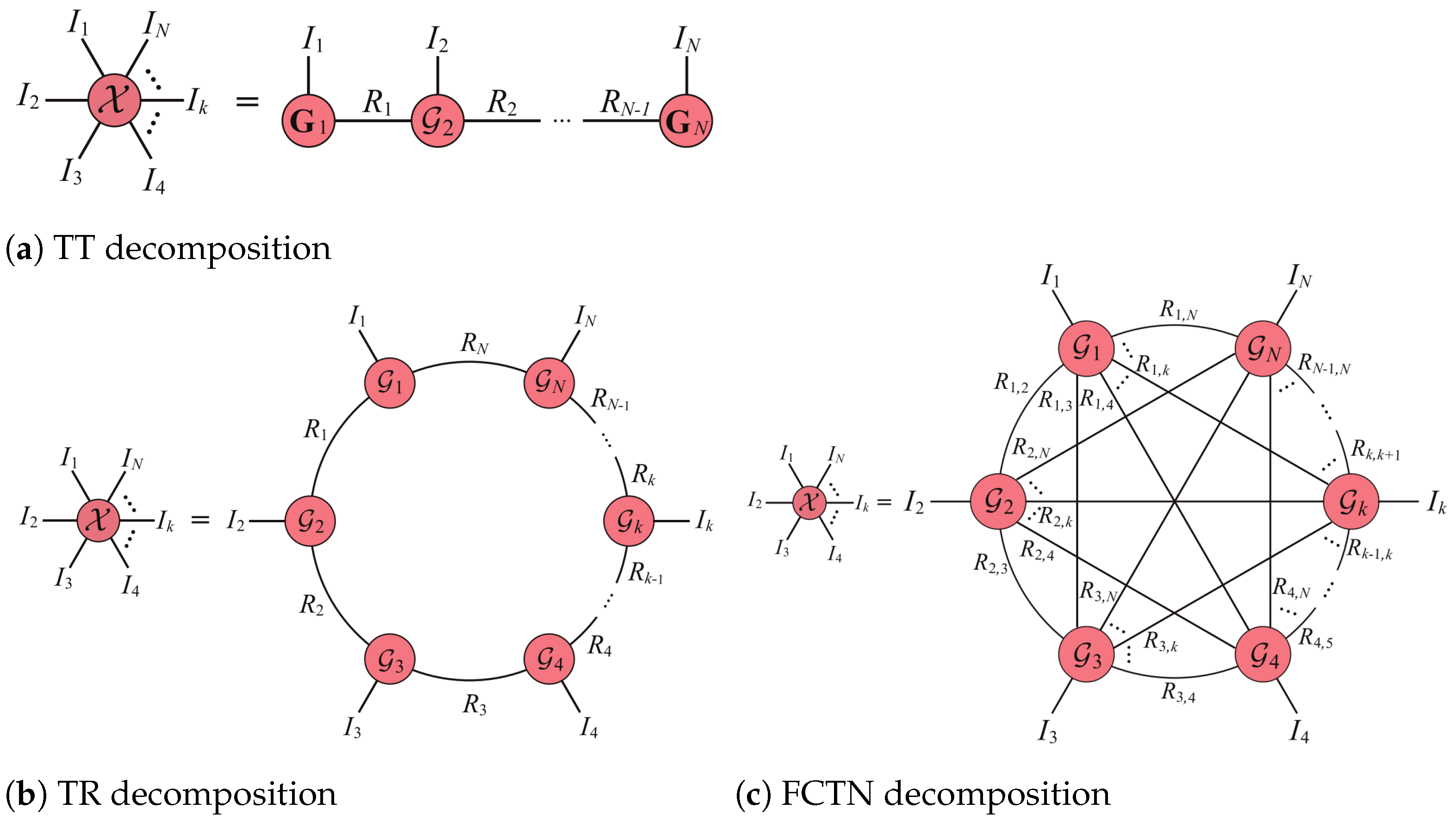
Figure 1. Depiction of tensor network decomposition.
Remotesensing 16 00034 g001
Figure 2. Clustering and separated target images obtained using different patch sizes.
Remotesensing 16 00034 g002
Figure 3. Illustration of the sensitivity of the detection results to the sliding window size: (a) two original images with similar complexity(b) results of superpixel segmentation and (c) ROC curves obtained with sliding windows of different sizes.
Remotesensing 16 00034 g003
Figure 4. The whole process of sliding window selection for adaptive superpixel segmentation.
Remotesensing 16 00034 g004
Figure 5. Intra-cluster low-rank properties of different clusters (a) represents the original image, (b) represents the singular value curve of the point feature group tensor, (c) represents the singular value curve of the line feature group tensor, and (d) represents the singular value curve of the flat feature group tensor.
Remotesensing 16 00034 g005
Figure 7. Images (ae) represent five real sequences employed in the experiments.
Remotesensing 16 00034 g007
Figure 8. ROC curves for Sequences 1 and 4 with respect to varying parameters. The first row corresponds to Sequence 1, while the second row represents Sequence 4. Column 1 pertains to patch size N 1 , Column 2 encompasses different λ 1 values, Column 3 shows various L values, and Column 4 concerns the temporal size N 3 .
Remotesensing 16 00034 g008
Figure 9. Different scenes (af) and results (gl).
Remotesensing 16 00034 g009
Figure 10. Scenarios and outcomes related to noise. (af) represents the white Gaussian noise image with standard deviation 10 added, and (gl) represents its corresponding object detection results using the C4D-FCTN method. (mr) represents the white Gaussian noise image with standard deviation 10 added, and (sx) represents its corresponding object detection results using the C4D-FCTN method.
Remotesensing 16 00034 g010
Figure 11. Different testing methods were employed to detect the results on Sequences 1 to 5 in the three-dimensional surface.
Remotesensing 16 00034 g011
Figure 12. Detection outcomes for Sequences 1 to 5 employing seven different testing methodologies. The target is represented by a purple box, while a detection failure is indicated by a dotted box.
Remotesensing 16 00034 g012
Figure 13. ROC curves of the compared and proposed methods on different sequences.
Remotesensing 16 00034 g013
Figure 14. Detection results of the ablation study, showing ROC curves for 3DST-TCTN, 4D-FCTN, and C4D-FCTN on Sequences 1 to 5.
Remotesensing 16 00034 g014
Table 1. Data description (sizes in pixels).
Seq.Image SizeFramesAverage SCRTarget DescriptionBackground Description
1256 × 2563000.83Single, tiny, low nonlocal contrastArtifical structures, clutter
2256 × 2562006.08Small, slow-moving airplaneVillage, reflective road, forest
3256 × 2561000.71Small, slow-moving airplanevillage, reflective road, forest
4256 × 25630014.52Single, slow-moving airplaneForest, bright rock, noise
5256 × 2562007.55Small, dim, regular shapeRiver, noise, heavy clutter
Table 2. Parameter settings of the seven comparison methods.
MethodParameters
IPIPatch size: m 1 × n 1 : 50 × 50, sliding size: 10, λ = 1 / min m , n , ε = 1 × 10 7
RIPTPatch size: m × n : 30 × 30, sliding size: 10, λ = 1 / min m 1 , n 1 , ε = 1 × 10 7
PSTNNPatch size: m 1 × n 1 : 40 × 40, sliding size: 40, λ = 1 / max m 1 , n 1 n 3 , ε = 1 × 10 7
ECASTT β = 0.1 , t = 3, λ 1 = 0.009 , λ 2 = 5 / min ( m , n ) × t , λ 3 = 100 , ε = 1 × 10 7
MFSTPTPatch size: m 1 × n 1 : 60 × 60, sliding size: 60, λ = 1 / max ( n 1 , n 2 ) n 3
SRSTTL = 30, λ 1 = 0.05 , λ 2 = 0.1 , λ 3 = 100 , ε = 1 × 10 7 , μ = 0.01
OursPatch size: N 1 × N 2 , temporal size: N 3 = 20 , ε = 1 × 10 7
Table 3. Performance comparison of seven methods in terms of SCGR, BSF, CG, and LSNRG.
MethodSeq1Seq2Seq3Seq4Seq5
SCRGBSFSCRGBSFSCRGBSFSCRGBSFSCRGBSF
IPI7.632.388.637.635.302.8710.625.6225.647.17
ECASTT60.1615.8115.2923.4711.9126.4911.349.7584.6414.45
MFSTPT24.6019.96102.79295.1413.51207.241.020.6934.6812.45
PSTNN26.1723.300.9559.5582.4910.75274.3711.266.4525.45
RIPT6.711.3210.412.184.614.219.421.9215.149.65
SRSTT56.96262.48346.98245.78206.9794.5249.0998.9764.52246.54
Ours70.17221.32408.551330.8860.65301.44767.19374.3956.96285.62
MethodSeq1Seq2Seq3Seq4Seq5
CGLSNRGCGLSNRGCGLSNRGCGLSNRGCGLSNRG
IPI1.272.7519.541.431.101.221.902.731.2317.08
ECASTT032.671.351.301.211.1202.871.624.44
MFSTPT1.571.031.074.601.092.311.5701.0528.38
PSTNN0.112.870.180.070.030.050.1100.840.86
RIPT2.312.871.402.041.251.432.3001.314.27
SRSTT2.8347.081.2820.012.812.892.8701.568.36
Ours3.7568.452.2535.641.140.982.3247.081.604.62
Table 4. Comparison of average computing time (in seconds) of the seven methods.
MethodSeq1Seq2Seq3Seq4Seq5
IPI10.5311.70612.27217.34123.929
ECASTT9.20514.82315.00616.08713.821
MFSTPT0.9561.1031.0351.3240.998
PSTNN0.1130.1250.2130.3410.245
RIPT2.8002.3412.5152.6413.069
SRSTT18.62517.63319.56220.06517.326
Ours0.3510.2470.6500.3240.231
Disclaimer/Publisher’s Note: The statements, opinions and data contained in all publications are solely those of the individual author(s) and contributor(s) and not of MDPI and/or the editor(s). MDPI and/or the editor(s) disclaim responsibility for any injury to people or property resulting from any ideas, methods, instructions or products referred to in the content.