Abstract
Increasing evidence has shown that marine heatwaves (MHWs) have destructive impacts on marine ecosystems, and understanding the causes of these events is beneficial for mitigating the associated adverse effects on the provision of ecosystem services. During the 2019/20 boreal winter, a long-lasting extreme MHW event was recorded (over 90 days) in the Yellow Sea (YS). Observations and numerical experiments revealed that the unprecedented winter MHW event was initiated and sustained by a significant decrease in ocean heat loss in the YS, which may be associated with the pronounced weakening of the Siberian high system induced by an extreme positive Arctic Oscillation (AO) event. A weakened northerly wind is the essential prerequisite, while the extreme AO event is only a trigger for the winter MHW in the YS. It was also found that the extreme winter MHW event is likely to substantially affect the seasonal evolution of the vertical thermal structure, which may have a great impact on the whole ecosystem in the YS. This study provides new insights for the prediction of winter MHWs in the YS, as well as their effects on marine ecosystems in a changing climate.
1. Introduction
A marine heatwave (MHW) event is generally recognized as the prolonged abnormal or extreme warming of water temperature in the ocean [1]. An increasing occurrence of MHW events has been recorded in the past two decades and is predicted to continue globally under the current climate change [2]. The occurrence of MHW events results in substantial changes in the physical structure, biogeochemical cycling and species composition [3,4,5] and may even induce ecological catastrophes, such as coral bleaching, harmful algal blooms and fish deaths [6,7], threatening the biodiversity and health of ocean ecosystems and their services to human society. Understanding the formation mechanism of the MHW and its long-lasting impact would help improve its prediction and marine ecosystem management.
In recent years, an increasing number of MHW events have also been observed in the North Pacific Ocean. One particular event is “The Blob”, which occurred in the northeast of the Pacific Ocean off southern California during 2014–2015, which persisted for multiple years and caused extreme fish mortality and reproductive failure [8]. After half a decade, “The Blob” resurged, causing unprecedented upper ocean warming near the Gulf of Alaska in the summer of 2019 [9]. MHWs are also frequent visitors in the northwestern North Pacific. In the shelf seas of East Asia, MHWs occurred in three consecutive summers from 2016 to 2018 [10]. In the open ocean, extensive marine heatwaves were detected in the summer of 2021, which were the largest since 1982 in the context of intensity and extent [11].
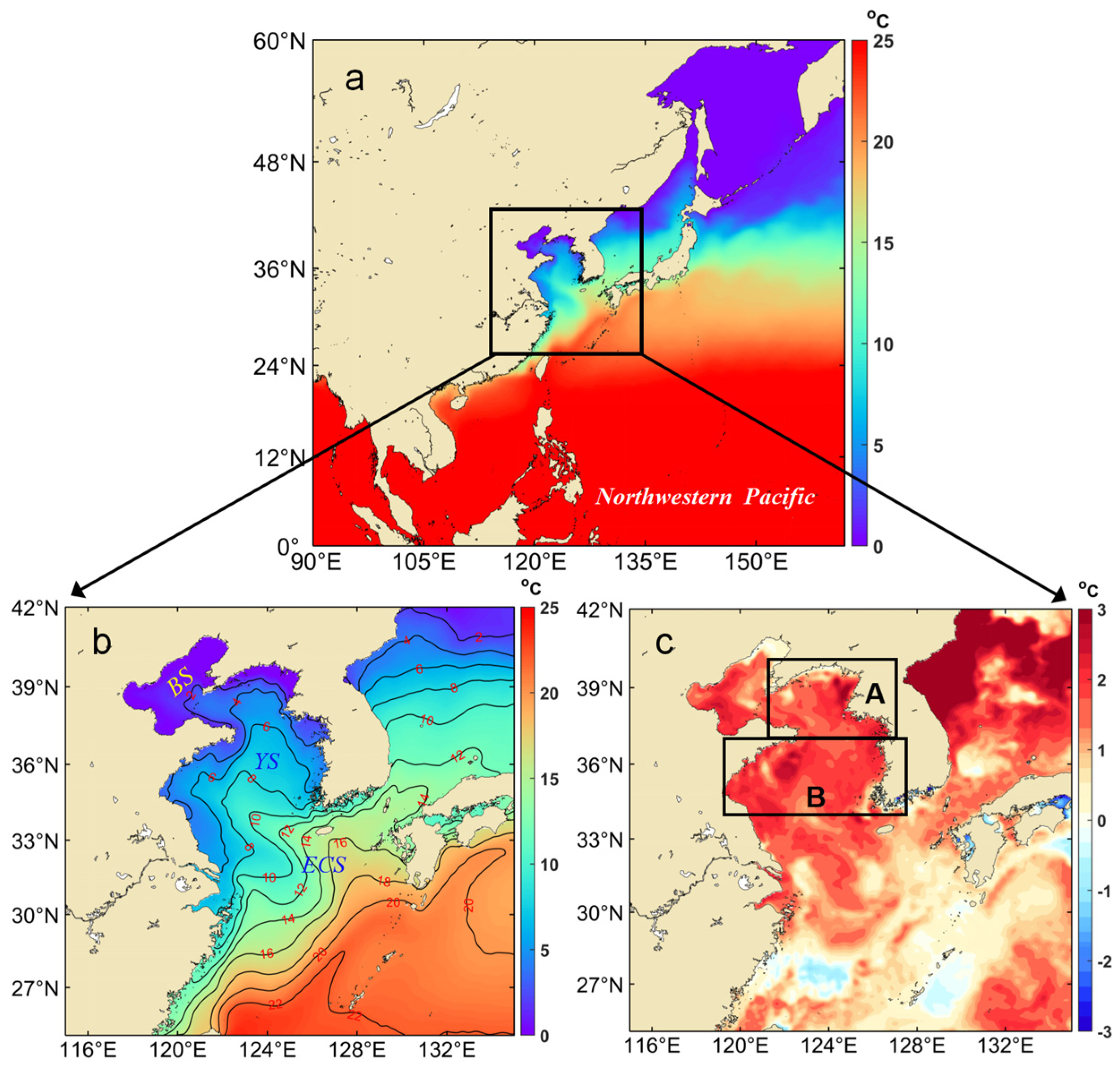
In the 2019/20 boreal winter, an extreme positive Arctic Oscillation (AO) event occurred and was found to be associated with multiple record-breaking phenomena in the polar and midlatitude regions. During or after the extreme AO, record ozone depletion in the Arctic was observed [12]. Siberia experienced an extreme heat wave with monthly air temperature anomalies over 6 °C in the following several months, and consequently, fires related to the extreme warming event burned an unprecedentedly large area of the Siberian Arctic since records began [13,14]. In East Asia, both the highest air temperature and sea surface temperature (SST) were found in the winter of 2019/20 [15]. Specifically, the winter mean SST anomaly reached over 1.5 ℃ in the Yellow Sea (hereafter referred to as the YS, Figure 1b). By MHW diagnosis, we identified that this is an extreme MHW event that lasted over 3 months.
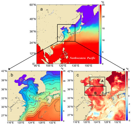
Figure 1.
(a) 40−year (1982–2021) averaged SST in February in the Northwest Pacific. (b) Same as (a) but for the shelf seas of East Asia, including the Bohai Sea (BS), Yellow Sea (YS) and East China Sea (ECS). (c) The monthly SST anomaly (relative to the 40 yr climatological mean) in February 2020. Black boxes A and B indicate the northern and southern YS, respectively. See Section 2.1 for a detailed data description.
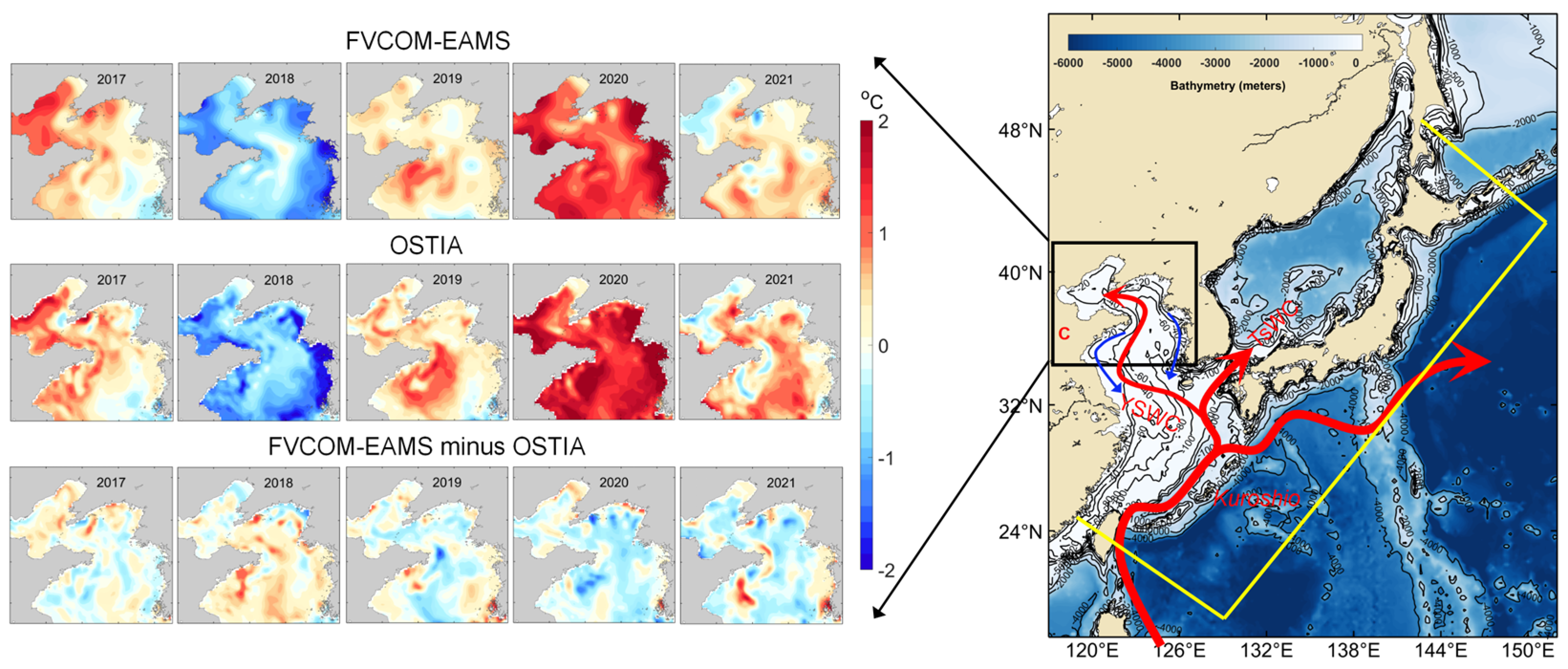
Due to shallow water depth (~44 m) and enhanced vertical mixing in winter, the oceanic water mass in the YS is vertically well-mixed. Therefore, two possible mechanisms can generally be used to explain the formation of extreme MHW events in the YS. One is the horizontal advection-induced heat transport by the Yellow Sea Warm Current (YSWC, Figure 2). The YSWC is a northward flow that can transport a large amount of warm water west of Cheju Island to the YS, contributing to a tongue-shaped warm water structure and its interannual variations [16,17]. Anomalous warm water transport may thus induce the abnormal warming of water temperature in the YS. Local air–sea interaction is another possible explanation for the formation of MHWs. For example, Yeh and Kim [18] demonstrated that the decreased latent and sensible heat flux induced by a weakened northerly wind was the main driver of the warming of winter SST during 1950–2008.
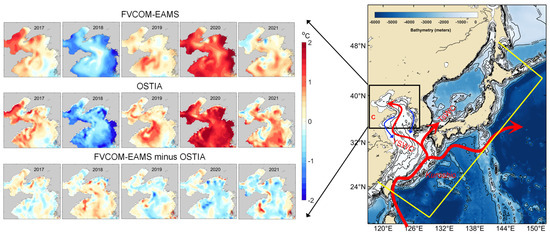
Figure 2.
(Right) Bathymetry (contours) and main currents (red and blue curves with arrows) in the model domain. YSWC and TsWC indicate the Yellow Sea Warm Current and Tsushima Warm Current, respectively. The blue curves with arrows represent the coastal currents. The area enclosed by the yellow lines represents the model domain. (Left) Comparison of FVCOM-EAMS monthly modeled SST anomaly with that of OSTIA in February in our study area (Right, c).
How was this extreme MHW event formed and would it have a long-lasting influence on the seasonal evolution of the water mass? By numerical simulation and diagnosis analysis, the dominant factors inducing the extreme winter MHW in the YS and its impact on the seasonal evolution of water temperature are investigated and discussed in this study. In Section 2, we introduce the data and methods. The characteristics, formation mechanism and consequences of this MHW event are demonstrated in Section 3. The evolution of MHWs and their potential impact on marine ecosystems, as well as their linkage with basin-scale climate variability, are discussed in Section 4. Our findings are summarized in Section 5.
2. Materials and Methods
2.1. Water Temperature and Meteorological Data
2.1.1. SST Data
In this study, the daily SST from the Operational SST and Sea Ice Analysis (OSTIA, [19], https://doi.org/10.48670/moi-00168, accessed on 11 November 2022) system is used for model validation and identification of MHW events in the YS. It is a Level-4 reprocessed product using in situ and satellite data with a 0.05° × 0.05° horizontal grid resolution. The temporal extent is from 1 January 1982 to 31 December 2021. The OSTIA SST data have been shown to be more accurate than other SST products in the YS [20].
2.1.2. Sea Bottom Temperature Data
The observed bottom water temperatures in the eastern YS from the Korea Oceanographic Data Center (KODC, https://www.nifs.go.kr/kodc/eng/eng_soo_list.kodc, accessed on 11 November 2022) are also used for model validation and analysis. The KODC provides the observed bottom water temperature 6 times/year (Feb., Apr., Jun., Aug., Oct., and Dec.), and observations from stations of Lines 307–311 (refer to Figure 3c) during 2012–2021 are used to validate the model performance in bottom temperature modeling.
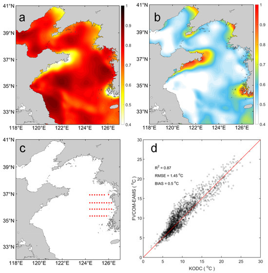
Figure 3.
(a) Correlation coefficients between the modeled monthly SST anomaly and that of OSTIA in the YS. (b) Same as (a) but for root mean square errors (RMSE). (c) Observation stations from the KODC. (d) Comparison of the modeled bottom temperature and that from KODC observations.
2.1.3. Meteorological Data
Meteorological data, including sea-level pressure (SLP), air temperature, precipitation, evaporation, wind speed, and heat flux, are compiled from 6-hourly products of the Climate Forecast System Reanalysis (CFSR and CFSv2, Saha et al., 2011) provided by the National Center for Environmental Prediction (NCEP) to drive the hydrodynamic model and to explain the MHW events. The temporal extent of the CFSR outputs is from 1 January 1982 to 31 December 2021. The horizontal grid resolution of the CFSR outputs ranges from 0.205° × 0.205° to 1.0° × 1.0°, which is distinct for each meteorological component.
2.2. Model Configuration and Validation
A hydrodynamic model named FVCOM-EAMS (Finite Volume Community Ocean Model applied in East Asian Marginal Seas) was used to derive the water temperature and current evolution that were used for further analysis. The bathymetry, computational domain and triangular grid design of FVCOM-EAMS can be seen in Yu et al. [21]. The horizontal resolution of the model grids is approximately 10 km in the YS, and 31 terrain-following sigma layers are designated in the vertical direction. The water temperature and salinity from HYCOM daily outputs (https://www.hycom.org/dataserver/gofs-3pt0/analysis, accessed on 11 November 2022) are interpolated into the FVCOM-EAMS triangular grids to generate the initial thermohaline conditions. The forcing in the open boundary includes subtidal sea surface height, temperature, salinity and currents, which are also derived from HYCOM outputs. Meanwhile, the hourly tidal fluctuations derived from the Tidal Model Driver (TMD, [22]) with 8 main tidal constituents (M2, S2, O1, K1, P1, Q1, N2, K2) are used for tidal forcing in the open boundary. For atmospheric forcing, the CFSR meteorological data are used to drive FVCOM-EAMS, including air pressure, precipitation, evaporation, wind stress and heat flux. The background vertical mixing coefficient is 1.0 × 10⁻⁵, and we use the Mellor and Yamada level 2.5 turbulent closure scheme for vertical mixing and the Smagorinsky turbulent closure scheme for horizontal mixing. Different from our previous work [21], no data assimilation techniques are implemented. The model was run from 1 January 2010 to 1 January 2022, and the model outputs from 2012 to 2021 were used for analysis. Figure 2 shows the comparison of the OSTIA- and FVCOM-EAMS-modeled monthly SST anomaly (relative to the 10 yr mean from 2012 to 2021) distribution in February in the YS. It is clear that the FVCOM-EAMS model can reproduce the interannual variability in winter SST well in the YS, especially for the higher SST during the 2019/2020 extreme MHW event. Additionally, the correlation coefficients between the modeled and observed monthly SST anomalies are higher than 0.7, and the RMSE is lower than 0.6 ℃ in most areas of the YS, except for some coastal regions (Figure 3a,b) in which the higher modeled errors may be induced by the imperfect parameterization scheme. Overall, the FVCOM-EAMS can well reproduce the interannual variation in SST in the YS. In addition, the modeled bottom water temperature corresponds well with the KODC observations (Figure 3d).
2.3. Definition of an MHW Event
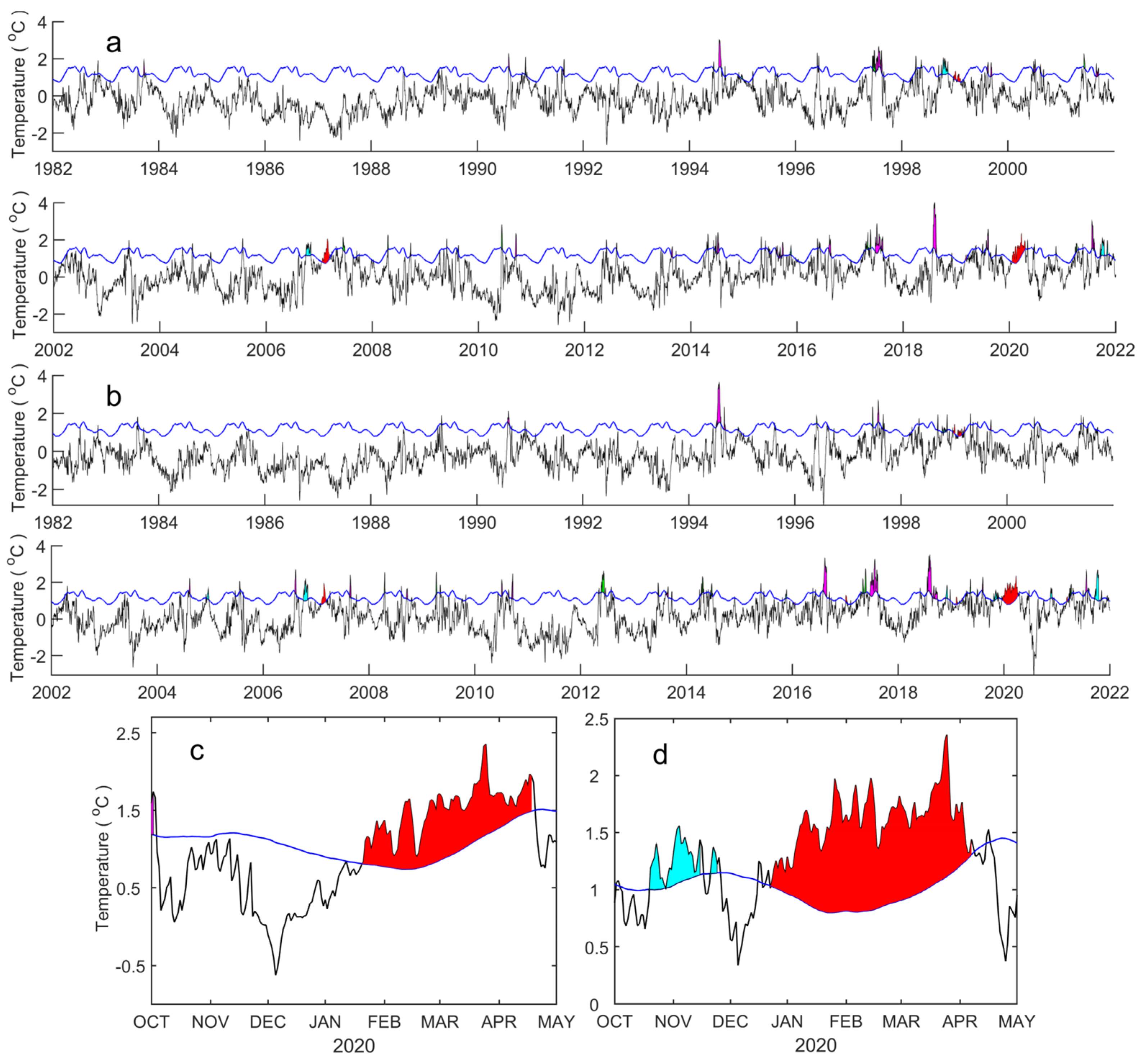
An MHW event is quantitatively described as a period in which the temperature continuously exceeds the 90th percentile of the daily temperature variations for at least 5 days over a period of 40 years (1982–2021) within an 11-day window centered on a specific date [1]. Based on the definition of Hobday et al. [1], three MHW metrics were adopted to further investigate their variations, including the duration (days between the start and end dates), the maximum intensity (maximum SST anomalies during a single event) and the cumulative intensity (sum of daily SST anomalies). The MHW events were detected using the averaged SST in boxes A and B, respectively.
2.4. Diagnosis Analysis
2.4.1. Temperature Change Induced by the Horizontal Advection Anomaly
As described above, horizontal advection and local heat flux are two main possible drivers influencing the interannual variability in winter water temperature in the YS. We first separate the whole YS into two parts (boxes A and B) to identify whether the mechanisms are the same for different regions. Considering that it is a long-lasting MHW event, we used a temperature budget method similar to Gao et al. [10] to investigate the influence of horizontal advection on the interannual variation in monthly water temperature in boxes A and B. For box A, the advection-induced temperature change can be described as
where represents the averaged water temperature change in box A solely induced by horizontal advection, is the water volume of box A, and represent the south and west boundaries of box A and and are the daily averaged meridional and zonal currents at the south and west boundaries, respectively. and are the daily average temperatures at the southern and western boundaries, respectively, and is the daily average temperature in box A. Similarly, the advection-induced temperature change in box B can be described as
where is the north boundary, represents the daily averaged meridional current at the north boundary and is the daily averaged temperature at the north boundary. The formulae are integrated for the whole water column in the vertical direction. We then calculated the cumulative daily and anomalies for further analysis, which represent the temperature change induced by the horizontal advection anomaly in boxes A and B.
2.4.2. Temperature Change Induced by Net Heat Flux Anomaly
The temperature change induced by the heat budget can be described as
where and are the density and specific heat capacity of sea water, respectively. represents the net heat flux, which is the summation of shortwave radiation absorbed in the whole water column , longwave radiation , sensible heat flux and latent heat flux . and are the water depth and area, respectively. The cumulative daily anomaly representing the temperature change induced by the net heat flux anomaly is then used for diagnosis analysis. After that, the interannual fluctuation of net heat flux as well as its components in the YS are detected, including solar radiation, longwave radiation and latent and sensible heat flux. The linkage of the net heat flux with basin-scale climate variability is then investigated.
3. Results
3.1. Characteristics of the Winter MHW Event in the YS
We first detected the MHWs based on the OSTIA data. Overall, the number of MHW events that occurred in winter (December to March) was much lower than that in summer. In the southern YS, 14 winter MHW events were detected during 1982–2021 (Table 1). Comparatively, only eight winter MHW events were identified in the northern YS (Table 2). Taking the duration and cumulative intensity into consideration, the winter 2019/2020 MHW event broke the record in both the northern and southern YS. The durations of this extreme MHW event in the northern and southern YS are 90 and 107 days, respectively (Figure 4). Meanwhile, two other strong MHW events, which occurred simultaneously in the northern and southern YS, were identified in the 1998/1999 (from December to March) and 2007 (from January to March) winters (Table 1 and Table 2).

Table 1.
Duration, maximum and cumulative intensity of the winter MHWs for box B.

Table 2.
Same as Table 1 but for Box A.
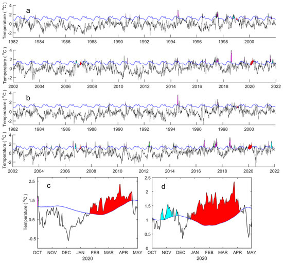
Figure 4.
(a) Time-varying MHWs in the northern YS (box A in Figure 1c) during 1982−2021. (b) Same as (a) but for the southern YS (box B in Figure 1c). The black and blue lines indicate SST anomalies and 90th percentile seasonally varying thresholds relative to the climatological daily mean. The color-filled areas represent MHWs (red for winter, green for spring, magenta for summer and cyan for autumn). (c,d) are the same as (a,b) but for the magnified SST anomalies from Oct 2019 to May 2020, respectively. Detailed information on the MHWs can be seen in Table 1 and Table 2.
3.2. Dominant Factors/Processes of Extreme MHWs in the YS
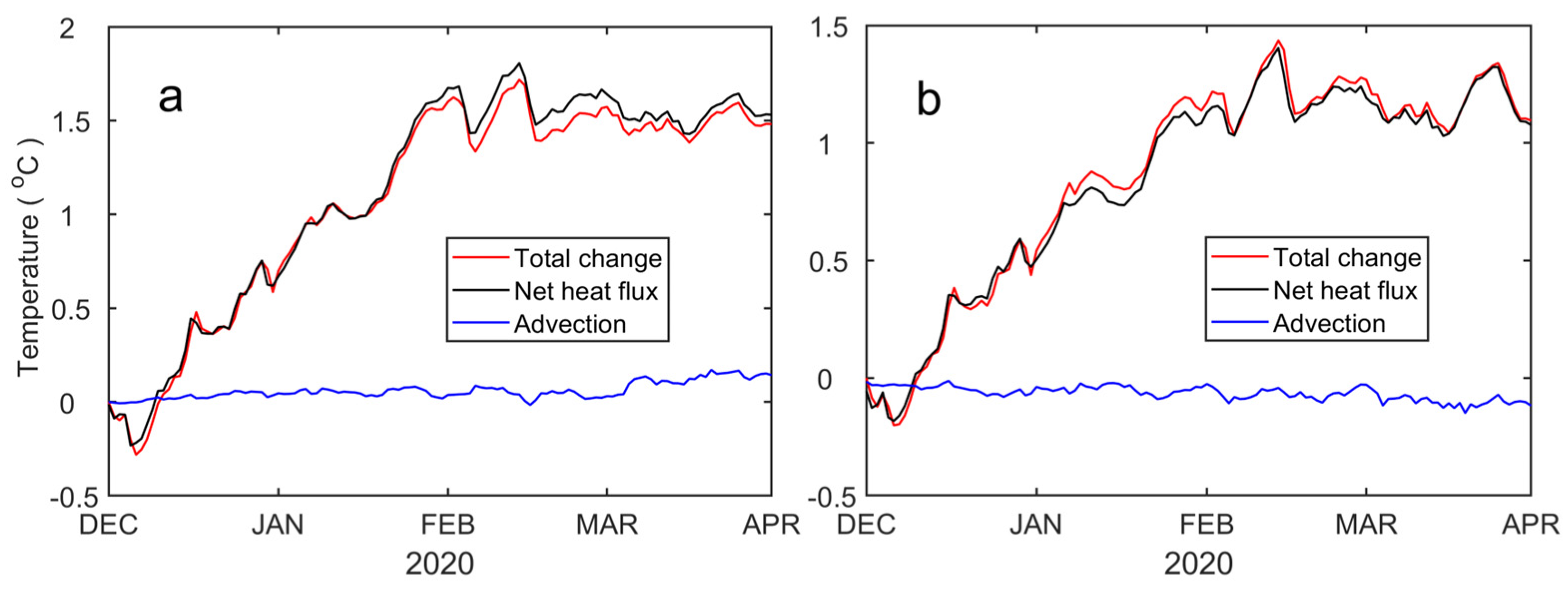
Figure 5 shows the time evolution of the modeled water temperature anomaly and that induced by the net heat flux and advection anomaly derived from diagnosis analysis. The modeled temperature anomaly grew from early December 2019 and reached its peak in early February 2020, which is consistent with the temperature anomaly induced by the net heat flux. It is clear that the local surface heat flux is the major cause of the water temperature anomaly during the boreal winter 2019–2020, while the effect of horizontal advection induced by the YSWC anomaly is negligible. Therefore, it can be concluded that local air–sea interaction determined the extreme MHW event in the YS.
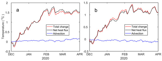
Figure 5.
(a) Time evolution of the modeled water temperature anomaly (red line) and cumulative water temperature changes (relative to 1 December 2019) caused by the net heat flux anomaly (black line) and horizontal advection anomaly (blue line) in box A. These anomalies are relative to the 10 yr mean value during 2012−2021. (b) Same as (a) but for box B.
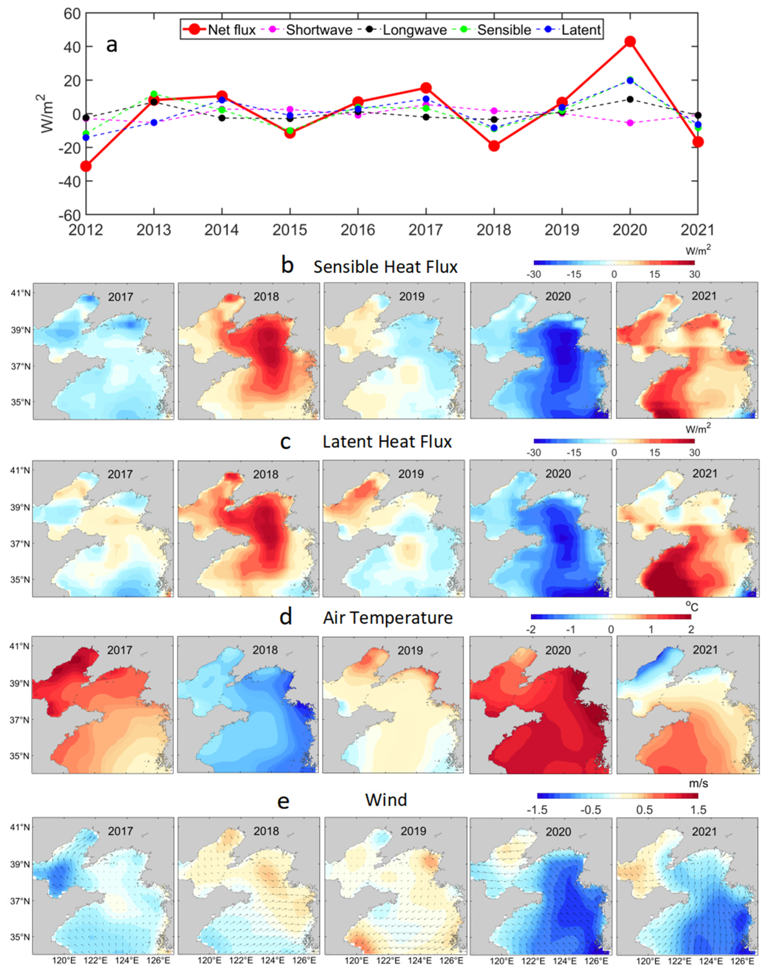
Interannual variations in the winter net heat flux and its components in the YS (Figure 6) were then detected. Obviously, the shortwave and longwave radiations did not show any considerable interannual variation. However, the net heat flux and sensible and latent heat fluxes in the 2019/20 winter were all higher than those in other years (Figure 6a). The decreased sensible and latent heat loss (Figure 6b,c) associated with the weakened winter monsoon and higher air temperature (Figure 6d,e) imply that more heat would be retained in the ocean, resulting in the extreme MHW event in the YS in winter 2019/20.
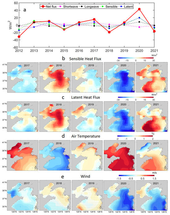
Figure 6.
(a) Interannual variation in the spatially averaged winter (December, January and February) mean net heat flux anomalies and their components in the YS during 2012−2021. Positive (negative) values indicate that more (less) heat is retained in the ocean. (b) Winter mean sensible heat flux (from ocean to atmosphere) during 2017−2021. (c–e) are the same as (b) but for latent heat flux, 2 m air temperature and 10 m wind, respectively.
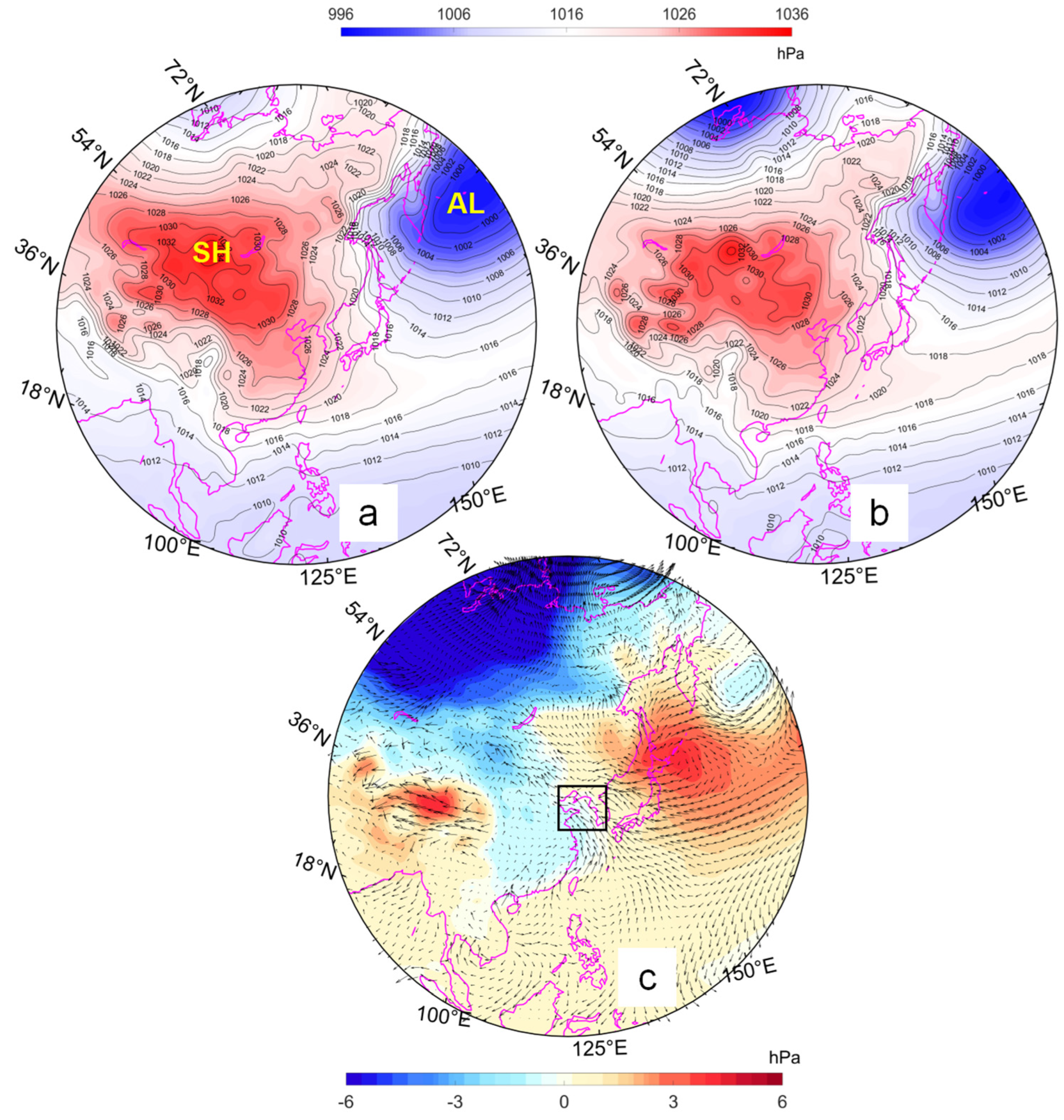
Figure 7 shows that the SLPs in the polar region, Siberia and eastern China during the extreme AO event were much lower in winter 2019/20. Specifically, the intensity of the Siberian high was significantly decreased. In contrast, the SLPs in the North Pacific and Japan in winter 2019/20 were higher than the 40 yr averaged winter SLPs. The dipole-like SLP anomaly pattern decreased the SLP gradient between Siberia and the shelf seas of East Asia, leading to the weakened northerly monsoon and the reduced cold advection from the continent in winter 2019/20.

Figure 7.
(a) 40−year winter (December, January and February during 1982–2021) mean SLP in East Asia. SH and AL represent the Siberian high and Aleutian low, respectively. (b) Same as (a) but for the 2019/2020 winter. (c) SLP (color fill) and wind (vectors) anomalies in the 2019/20 winter. The black box indicates the YS.
3.3. Impact of the Extreme MHW Event on the Seasonal Evolution of Water Temperature
As described in Figure 3d, FVCOM-EAMS can well reproduce the evolution of bottom water temperature. We then compared the observed and modeled bottom temperatures in the eastern YS. Generally, the observed mean bottom temperature during normal years (2012–2019, 2021) was lower than that in 2020 (Figure 8a). Note that the bottom temperatures in some survey stations in August and October in 2020 were relatively lower, which may be associated with the lower temperature in the upper ocean in summer (Figure 8c). Overall, the observed bottom temperatures in 2020 were more than 1℃ higher than those in normal years in all seasons (Table 3). For the FVCOM-EAMS model results, all the bottom temperatures in 2020 were relatively higher than those in normal years (Figure 8b). Despite that, since the differences between KODS and the FVCOM-EAMS model (Table 3) are several times less than the differences between normal and MHW years, the FVCOM-EAMS can well reproduce the warming of the bottom temperature, as well as its seasonal evolution in the YS.
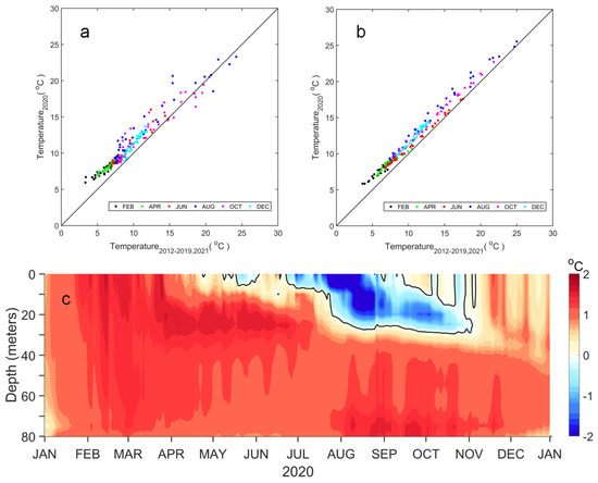
Figure 8.
(a) Observed mean bottom temperature of normal years (2012–2019, 2021) versus the observed bottom temperature in 2020. Each dot indicates the observation at each station in Figure 3c in a specific month. (b) Same as (a) but for model results. (c) The FVCOM–EAMS–derived seasonal evolution of the vertical thermal structure anomaly in 2020 in the southern YS (box B).

Table 3.
Averaged bottom temperature anomaly for KODC stations in 2020.
Figure 8c shows the FVCOM-EAMS-derived seasonal evolution of the vertical thermal structure anomaly in southern YS in 2020. The temperature of the whole water column during January–March 2020 was higher than that of normal years. The temperature of the upper ocean became normal in early April, while that in the subsurface and bottom layers was still warmer than that in normal years. Comparatively, the warming of the subsurface water temperature was greater than that of bottom water during April–July. During July–October, the water temperature at the surface (20 m) was lower than that of normal years, especially in July and August. However, the bottom temperature anomalies became much higher during August–October than those in winter and spring. Overall, the warmer subsurface and bottom water that formed during the MHW event may have contributed a lot to the higher water temperature in the subsurface and bottom layers during its seasonal evolution. As the following winter comes, the higher bottom temperature will contribute to a relatively warmer SST due to strong vertical mixing in winter.
4. Discussion
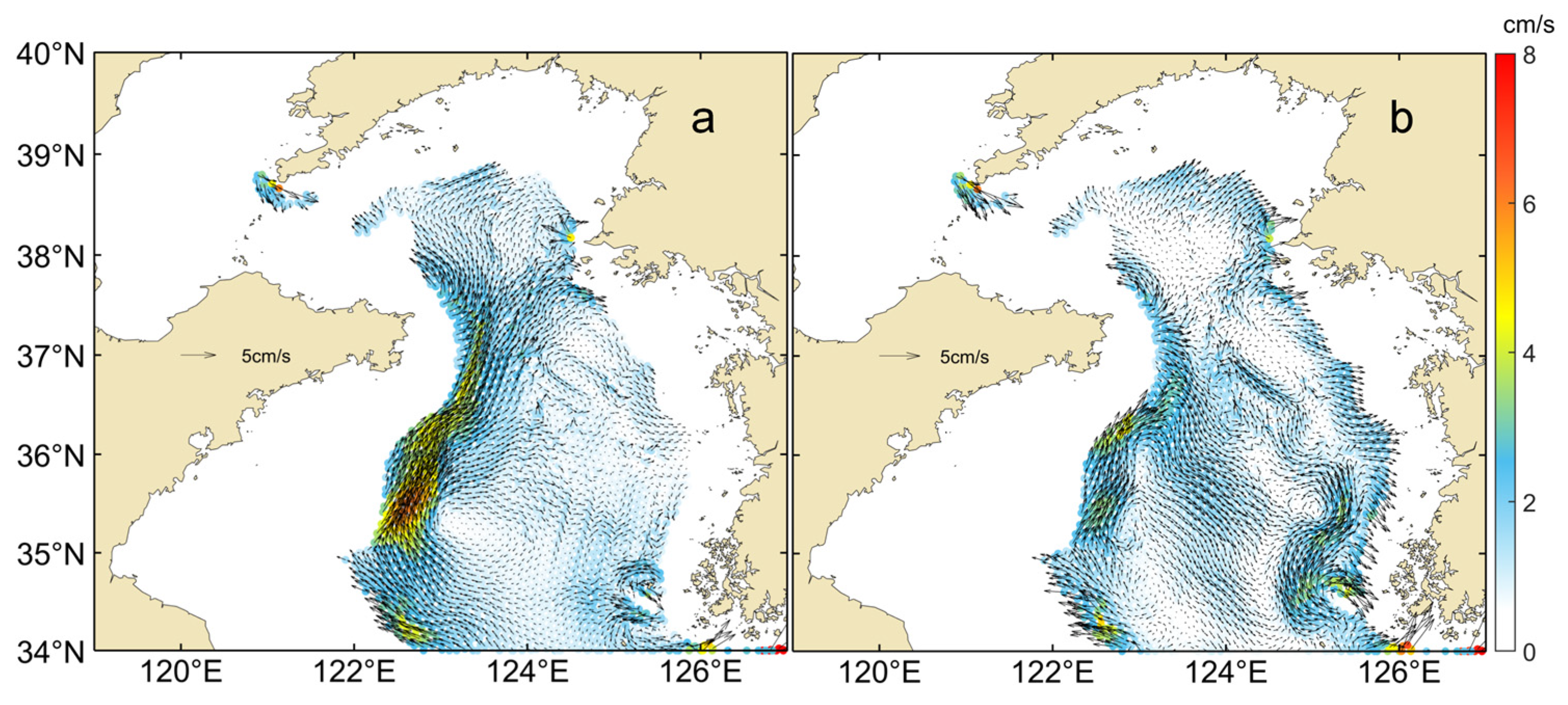
The FVCOM-EAMS model can also well reproduce the YSWC pathway compared with the observations [23], and it seems that the YSWC became weak during 2019/20 winter (Figure 9). Despite that, by diagnosis analysis, it was found that the air–sea heat flux plays an important role in winter temperature evolution, while the role of the YSWC is negligible, although the YSWC generally contributes to the winter SST distribution in the YS [17]. It can then be inferred that the interannual variation in winter SST was strongly associated with climate variability. This study provides a typical example for this inference, as we proved that the weakened wind that is associated with large-scale climate variability would help retain more heat in the ocean, which triggered the extreme MHW event in the YS. The degradation of the MHW event may be related to a large amount of latent heat release in April [24]. In contrast to winter seasons, however, horizontal advection may play a more important role in SST variations and the formation of MHW events in summer [10,25], indicating that the physical mechanisms of MHWs in the YS are somewhat different in different seasons.

Figure 9.
(a) The modeled 10 yr winter (December, January and February) with 50 m mean currents. (b) Same as (a) but for 2020.
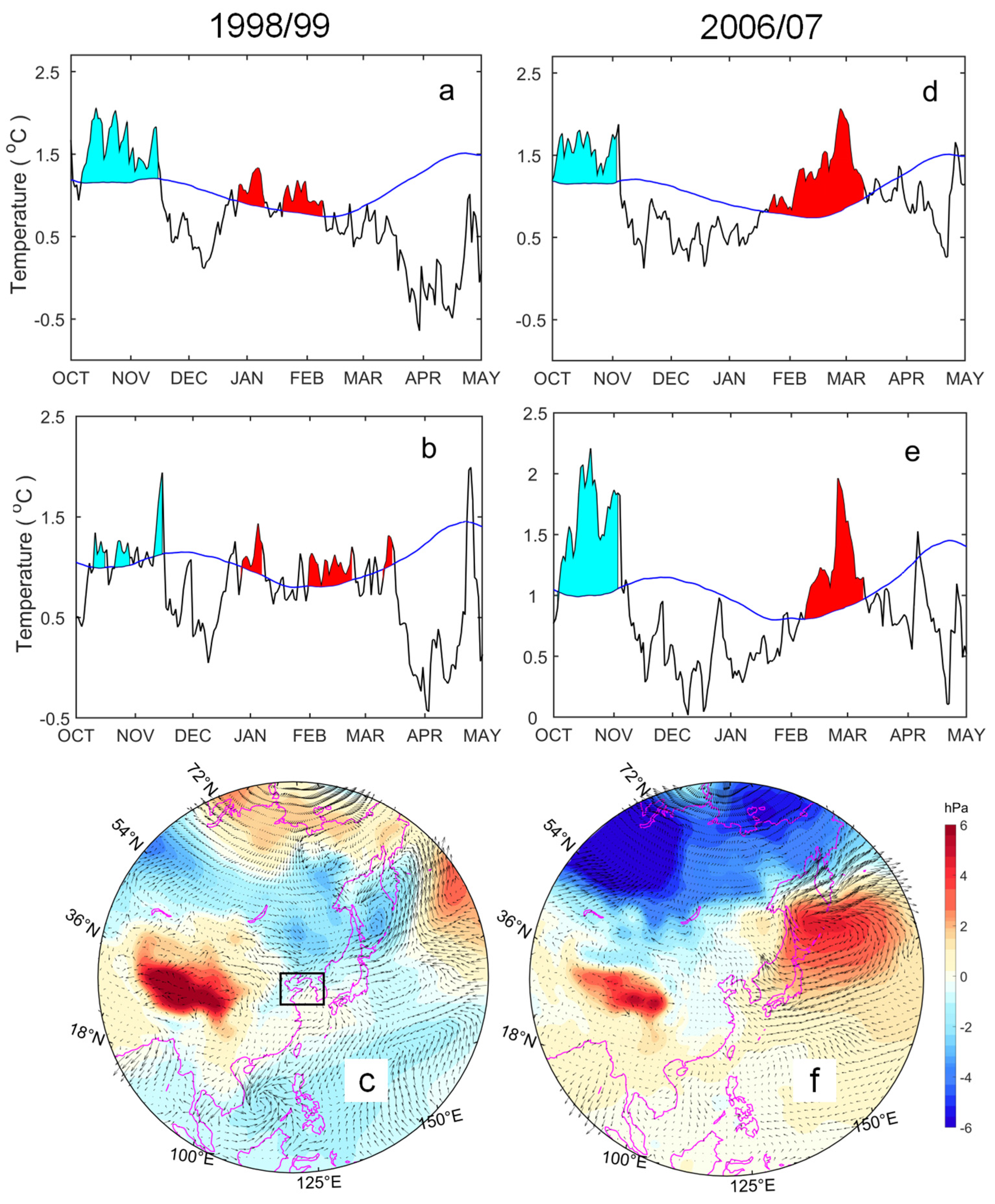
A previous study proved that an extreme AO event contributed a lot to the higher air and water temperature in winter 2019/20 in East Asia [15]. In the 1998/99 and 2007 winters, the YS also experienced two striking MHW events, and similarly, the wind in these two winters was also weakened (Figure 9). However, their linkages with anomalous large-scale atmospheric circulation are different. In winter 1998/99, an anomalous anticyclone emerged in the YS, resulting in a decreased wind speed in the YS (Figure 10c). In contrast, the weakened northerly wind in winter 2007 may have resulted from an extreme AO event, which was similar to that in winter 2019/20 (Figure 10f). It should be noted that not all extreme AO events can trigger an MHW event in the YS. For instance, an extreme AO event occurred in winter 1988/89, but the winter SST in the YS was not as high as expected (Figure 11a,b). An anomalous cyclone occurred in the YS in winter 1988/89, which seems to have been associated with the weakened Aleutian low (Figure 11c). The relationships between large-scale atmospheric circulation and local wind in the YS should be further investigated to clarify the underlying mechanisms of winter MHWs in the YS in a changing climate.
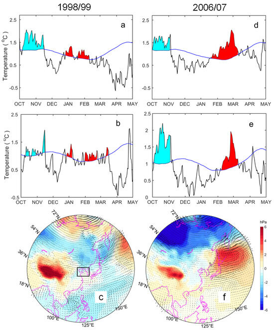
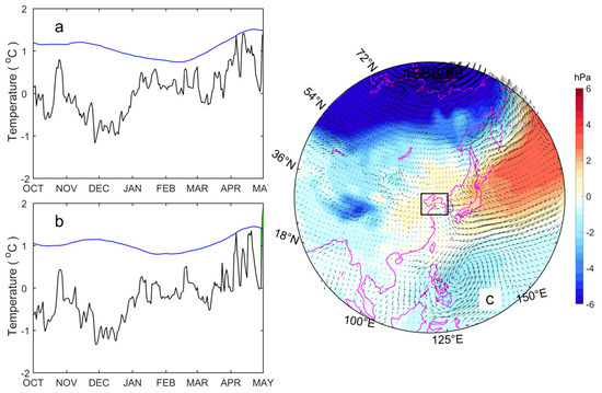
Figure 11.
(a–c) Same as Figure 10 (a–c) but for winter 1988/89. The black box indicates the YS.
The extreme MHW in winter 2019/20 in the YS resulted in a substantial change in the seasonal evolution of the vertical thermal structure in 2020, which may provide a precondition for some striking ecological phenomena in the following spring and summer. For example, Kim et al. [24] reported that the warm temperature in winter and enhanced release of latent heat fluxes in spring contribute to the unprecedented retardation of spring water temperature rise in the northern YS, inducing weakened vertical stratification and further delaying and suppressing spring phytoplankton blooms. Although Yoon et al. [26] demonstrated that the decline in phytoplankton biomass (~30%) during February–May 2020 was related to the decreased atmospheric nutrient deposition associated with the COVID-19 lockdown, the weakened stratification may also have played a significant role in suppressing primary production. A physical–ecological model may help identify the influence of human activities and climate-induced MHWs on marine ecosystems.
5. Conclusions
An extreme MHW event that lasted over 90 days was identified in the YS in winter 2019/20, and it was successfully reproduced by a hydrodynamic model. By diagnosis analysis, we demonstrated that the significantly decreased air–sea heat flux led to this MHW event rather than heat transport by the YSWC. The decreased air–sea heat flux (i.e., sensible and latent heat flux) was associated with the weakened wind speed, which may be related to the pronounced weakening of the Siberian high system and the extreme AO event. However, the extreme AO event was not an essential prerequisite for the winter MHW in the YS, while all of the extreme winter MHW events in the YS were associated with the significantly decreased northerly wind speed. This extreme MHW event induced a substantial change in the seasonal evolution of the vertical thermal structure, which may have contributed to the striking suppression of phytoplankton spring blooms in the YS in 2020.
Author Contributions
Conceptualization, H.Y. and L.J.; methodology, H.Y. and Q.X.; software, H.Y. and Q.X.; validation, H.W., L.J. and J.M.; formal analysis, H.Y.; investigation, L.J. and H.Y.; resources, L.J., H.W. and J.M.; data curation, H.Y. and Q.X.; writing—original draft preparation, H.Y.; writing—review and editing, H.W., L.J. and J.M.; visualization, H.Y.; supervision, H.W.; funding acquisition, L.J. and J.M. All authors have read and agreed to the published version of the manuscript.
Funding
This research was jointly funded by Shandong Provincial Natural Science Foundation (ZR2022QD041; ZR202211130079), the National Natural Science Foundation of China (42141001) and the China Postdoctoral Science Foundation (2021T140674).
Data Availability Statement
The OSTIA SST data can be freely obtained through https://data.marine.copernicus.eu/product/SST_GLO_SST_L4_REP_OBSERVATIONS_010_011/services (accessed on 11 November 2022). The observed Sea bottom temperature data were obtained from the Korea Oceanographic Data Center (KODC) at https://www.nifs.go.kr/kodc/eng/eng_soo_list.kodc (accessed on 11 November 2022). The meteorological data were provided by The National Centers for Environmental Prediction (NCEP) Climate Forecast System (CFS), which can be downloaded at https://rda.ucar.edu/datasets/ds094.0/index.html#!cgi-bin/datasets/getSubset?dsnum=094.0&action=customize&_da=y (accessed on 11 November 2022). The FVCOM simulation output and computing codes used in this study are available on request to the authors.
Conflicts of Interest
The authors declare no conflict of interest.
References
- Hobday, A.J.; Alexander, L.V.; Perkins, S.E.; Smale, D.A.; Straub, S.C.; Oliver, E.C.; Benthuysen, J.A.; Burrows, M.T.; Donat, M.G.; Feng, M.; et al. A hierarchical approach to defining marine heatwaves. Prog. Oceanogr. 2016, 141, 227–238. [Google Scholar] [CrossRef]
- Plecha, S.M.; Soares, P.M. Global marine heatwave events using the new CMIP6 multi-model ensemble: From shortcomings in present climate to future projections. Environ. Res. Lett. 2020, 15, 124058. [Google Scholar] [CrossRef]
- Schaeffer, A.; Roughan, M. Subsurface intensification of marine heatwaves off southeastern Australia: The role of stratification and local winds. Geophys. Res. Lett. 2017, 44, 5025–5033. [Google Scholar] [CrossRef]
- Frölicher, T.L.; Laufkötter, C. Emerging risks from marine heat waves. Nat. Commun. 2018, 9, 650. [Google Scholar] [CrossRef] [PubMed]
- Hayashida, H.; Matear, R.J.; Strutton, P.G. Background nutrient concentration determines phytoplankton bloom response to marine heatwaves. Glob. Chang. Biol. 2020, 26, 4800–4811. [Google Scholar] [CrossRef] [PubMed]
- Roberts, S.D.; Van Ruth, P.D.; Wilkinson, C.; Bastianello, S.S.; Bansemer, M.S. Marine heatwave, harmful algae blooms and an extensive fish kill event during 2013 in South Australia. Front. Mar. Sci. 2019, 6, 610. [Google Scholar] [CrossRef]
- Couch, C.S.; Burns, J.H.; Liu, G.; Steward, K.; Gutlay, T.N.; Kenyon, J.; Eakin, C.M.; Kosaki, R.K. Mass coral bleaching due to unprecedented marine heatwave in Papahānaumokuākea Marine National Monument (Northwestern Hawaiian Islands). PLoS ONE 2017, 12, e0185121. [Google Scholar] [CrossRef] [PubMed]
- Piatt, J.F.; Parrish, J.K.; Renner, H.M.; Schoen, S.K.; Jones, T.T.; Arimitsu, M.L.; Kuletz, K.J.; Bodenstein, B.; García-Reyes, M.; Duerr, R.S.; et al. Extreme mortality and reproductive failure of common murres resulting from the northeast Pacific marine heatwave of 2014–2016. PLoS ONE 2020, 15, e0226087. [Google Scholar] [CrossRef]
- Amaya, D.J.; Miller, A.J.; Xie, S.P.; Kosaka, Y. Physical drivers of the summer 2019 North Pacific marine heatwave. Nat. Commun. 2020, 11, 1903. [Google Scholar] [CrossRef]
- Gao, G.; Marin, M.; Feng, M.; Yin, B.; Yang, D.; Feng, X.; Ding, Y.; Song, D. Drivers of marine heatwaves in the East China Sea and the South Yellow Sea in three consecutive summers during 2016–2018. J. Geophys. Res. Ocean. 2020, 125, e2020JC016518. [Google Scholar] [CrossRef]
- Kuroda, H.; Setou, T. Extensive marine heatwaves at the sea surface in the northwestern Pacific Ocean in summer 2021. Remote Sens. 2021, 13, 3989. [Google Scholar] [CrossRef]
- Lawrence, Z.D.; Perlwitz, J.; Butler, A.H.; Manney, G.L.; Newman, P.A.; Lee, S.H.; Nash, E.R. The remarkably strong Arctic stratospheric polar vortex of winter 2020: Links to record-breaking Arctic oscillation and ozone loss. J. Geophys. Res. Atmos. 2020, 125, e2020JD033271. [Google Scholar] [CrossRef]
- Overland, J.E.; Wang, M. The 2020 Siberian heat wave. Int. J. Climatol. 2021, 41, E2341–E2346. [Google Scholar] [CrossRef]
- Descals, A.; Gaveau, D.L.; Verger, A.; Sheil, D.; Naito, D.; Peñuelas, J. Unprecedented fire activity above the Arctic Circle linked to rising temperatures. Science 2022, 378, 532–537. [Google Scholar] [CrossRef] [PubMed]
- Kim, S.H.; Kryjov, V.N.; Ahn, J.B. The roles of global warming and Arctic Oscillation in the winter 2020 extremes in East Asia. Environ. Res. Lett. 2022, 17, 065010. [Google Scholar] [CrossRef]
- Ma, J.; Qiao, F.; Xia, C.; Kim, C.S. Effects of the Yellow Sea Warm Current on the winter temperature distribution in a numerical model. J. Geophys. Res. Ocean. 2006, 111. [Google Scholar] [CrossRef]
- Wan, X.; Liu, S.; Ma, W. Numerical simulation of double warm tongues related to the bifurcation of the Yellow Sea warm current. Cont. Shelf Res. 2022, 236, 104680. [Google Scholar] [CrossRef]
- Yeh, S.W.; Kim, C.H. Recent warming in the Yellow/East China Sea during winter and the associated atmospheric circulation. Cont. Shelf Res. 2010, 30, 1428–1434. [Google Scholar] [CrossRef]
- Good, S.; Fiedler, E.; Mao, C.; Martin, M.J.; Maycock, A.; Reid, R.; Roberts-Jones, J.; Searle, T.; Waters, J.; While, J.; et al. The current configuration of the OSTIA system for operational production of foundation sea surface temperature and ice concentration analyses. Remote Sens. 2020, 12, 720. [Google Scholar] [CrossRef]
- Kwon, K.; Choi, B.J.; Kim, S.D.; Lee, S.H.; Park, K.A. Assessment and improvement of global gridded sea surface temperature datasets in the yellow sea using in situ ocean buoy and research vessel observations. Remote Sens. 2020, 12, 759. [Google Scholar] [CrossRef]
- Yu, H.; Yu, H.; Ito, S.I.; Tian, Y.; Wang, H.; Liu, Y.; Xing, Q.; Bakun, A.; Kelly, R.M. Potential environmental drivers of Japanese anchovy (Engraulis japonicus) recruitment in the Yellow Sea. J. Mar. Syst. 2020, 212, 103431. [Google Scholar] [CrossRef]
- Padman, L.; Erofeeva, S. Tide Model Driver (TMD) Manual; Earth and Space Research: Seattle, WA, USA, 2005. [Google Scholar]
- Lin, X.; Yang, J.; Guo, J.; Zhang, Z.; Yin, Y.; Song, X.; Zhang, X. An asymmetric upwind flow, Yellow Sea warm current: 1. New observations in the western Yellow Sea. J. Geophys. Res. Ocean. 2011, 116, C04026. [Google Scholar] [CrossRef]
- Kim, G.U.; Lee, K.; Lee, J.; Jeong, J.Y.; Lee, M.; Jang, C.J.; Ha, K.J.; Nam, S.; Noh, J.H.; Kim, Y.S. Record-breaking slow temperature evolution of spring water during 2020 and its impacts on spring bloom in the Yellow Sea. Front. Mar. Sci. 2022, 9, 824361. [Google Scholar] [CrossRef]
- Wang, B.; Wu, L. Sea surface temperature (SST) anomalies of the Yellow and East China Seas in July of 2020. In E3S Web of Conferences; EDP Sciences: Les Ulis, France, 2021; Volume 228, p. 02006. [Google Scholar]
- Yoon, J.E.; Son, S.; Kim, I.N. Capture of decline in spring phytoplankton biomass derived from COVID-19 lockdown effect in the Yellow Sea offshore waters. Mar. Pollut. Bull. 2022, 174, 113175. [Google Scholar] [CrossRef]
Disclaimer/Publisher’s Note: The statements, opinions and data contained in all publications are solely those of the individual author(s) and contributor(s) and not of MDPI and/or the editor(s). MDPI and/or the editor(s) disclaim responsibility for any injury to people or property resulting from any ideas, methods, instructions or products referred to in the content. |
© 2023 by the authors. Licensee MDPI, Basel, Switzerland. This article is an open access article distributed under the terms and conditions of the Creative Commons Attribution (CC BY) license (https://creativecommons.org/licenses/by/4.0/).

