Article

Estimation of Oak Leaf Functional Traits for California Woodland Savannas and Mixed Forests: Comparison between Statistical, Physical, and Hybrid Methods Using Spectroscopy

1
ONERA/DOTA, Université de Toulouse, F-31055 Toulouse, France
2
Faculty of Geo-Information Science and Earth Observation (ITC), University of Twente, 7522 NH Enschede, The Netherlands
3
Institute of the Environment, University of California Davis, Davis, CA 95616, USA
*
Author to whom correspondence should be addressed.
Remote Sens. 2024, 16(1), 29; https://doi.org/10.3390/rs16010029
Submission received: 4 October 2023 / Revised: 12 December 2023 / Accepted: 14 December 2023 / Published: 20 December 2023

Abstract

:
Key leaf functional traits, such as chlorophyll and carotenoids content (Cab and Cxc), equivalent water thickness (EWT), and leaf mass per area (LMA), are essential to the characterization and monitoring of ecosystem function. Spectroscopy provides access to these four leaf traits by relying on their specific spectral absorptions over the 0.4–2.5 µm domain. In this study, we compare the performance of three categories of estimation methods to retrieve these four leaf traits from laboratory directional-hemispherical leaf reflectance and transmittance measurements: statistical, physical, and hybrid methods. To this aim, a dataset pooling samples from 114 deciduous and evergreen oak trees was collected on four sites in California (woodland savannas and mixed forests) over three seasons (spring, summer and fall) and was used to assess the performance of each method. Physical and hybrid methods were based on the PROSPECT leaf radiative transfer model. Physical methods included inversion of PROSPECT from iterative algorithms and look-up table (LUT)-based inversion. For LUT-based methods, two distance functions and two sampling schemes were tested. For statistical and hybrid methods, four distinct machine learning regression algorithms were compared: ridge, partial least squares regression (PLSR), Gaussian process regression (GPR), and random forest regression (RFR). In addition, we evaluated the transferability of statistical methods using an independent dataset (ANGERS Leaf optical properties database) to train the regression algorithms. Thus, a total of 17 estimations were compared. Firstly, we studied the PROSPECT leaf structural parameter N retrieved by iterative inversions and its distribution over our oak-specific dataset. N showed a more pronounced seasonal dependency for the deciduous species than for the evergreen species. For the four traits, the statistical methods trained on our dataset outperformed the PROSPECT-based methods. More particularly, statistical methods using GPR yielded the most accurate estimates (RMSE = 5.0 µg·cm−2; 1.3 µg·cm−2; 0.0009 cm; and 0.0009 g·cm−2 for Cab, Cxc, EWT, and LMA, respectively). Among the PROSPECT-based methods, the iterative inversion of this model led to the most accurate results for Cab, Cxc, and EWT (RMSE = 7.8 µg·cm−2; 2.0 µg·cm−2; and 0.0035 cm, respectively), while for LMA, a hybrid method with RFR (RMSE = 0.0030 g·cm−2) was the most accurate. These results showed that estimation accuracy is independent of the season. Considering the transferability of statistical methods, for the four leaf traits, estimation performance was inferior for estimators built on the ANGERS database compared to estimators built exclusively on our dataset. However, for EWT and LMA, we demonstrated that these types of statistical methods lead to better estimation accuracy than PROSPECT-based methods (RMSE = 0.0016 cm and 0.0013 g·cm−2 respectively). Finally, our results showed that more differences were observed between plant functional types than between species or seasons.

1. Introduction

Oak trees from the Quercus genus comprise around 500 species, including both deciduous and evergreen species. They are mostly distributed in the Northern Hemisphere from cool temperate to tropical climates, and their numbers are the greatest in North America and China. According to the Red List of Oak 2020 report and analyses of over 430 species studied worldwide, about 31% of oak species are estimated to be threatened and globally, 41% are considered to be of conservation concern [1]. They are mainly endangered by land use change due to agriculture and urbanization expansion, as well as logging and global climate change, which is leading to a decrease in water availability and increase in fires, pests, and diseases. However, oak trees are of high ecological and economic importance since they provide food (acorns) and habitat for fauna, serve as carbon sinks, and are used for timber, furniture, fuel, dyes, and tannins [2]. They are present in 18 out of the 36 biodiversity hotspots recognized by the Critical Ecosystem Partnership Fund (CEPF), which feature a rich biodiversity but experience severe habitat loss. About 89 oak species exist in the United States and 20 are present in California, of which 7 are endemic [3]. Oak trees are distributed between oak woodland savannas and oak forest ecosystems, the former representing about 50,000 km2 while the latter 27,000 km2 [4]. Most are threatened due to population increase and demand for wood and fuel; management plans have been drawn up for the six regions of California to preserve oak resources, promote stand regeneration, and prevent fire propagation [5].
Optical remote sensing is a widely used technology to observe large-scale terrestrial landscapes with high temporal revisit. Remote sensing has been used to observe oak ecosystems: for instance, for monitoring the spatio-temporal land cover change of a cork oak forest due to anthropogenic disturbance [6], for assessing the post-fire recovery of a mixed pine–oak forest [7], for estimating tree cover over an evergreen oak woodland [8], and for identifying pest-infected oak trees [9]. The remotely sensed signal acquired at the top of a tree canopy is to a certain extent influenced by canopy structure, but primarily by leaf reflectance and transmittance. These optical properties have been demonstrated to be the expression of plant functions and strategies [10]. The latter can be explained through the definition of plant traits and plant functional traits, which can be upscaled from the individual to the ecosystem level. A plant trait is any morphological, physiological, or phenological feature measurable without reference to the environment, while a functional trait is any trait that impacts fitness indirectly via its effects on growth, reproduction, and survival [11].
Among the optically relevant traits at the leaf level, chlorophyll a and b content (Cab), carotenoid content (Cxc), equivalent water thickness (EWT), and leaf mass area (LMA) are often studied since they have been proven to be valuable indicators to assess vegetation health and stress levels [12].
Due to their biochemical (Cab, Cxc, EWT) or morphological nature (LMA), they have become fundamental for monitoring environmental function and structure in order to improve our understanding of physiological vegetation processes and global biogeochemical cycles [13]. Monitoring leaf traits would also provide insight into vegetation resilience against the increased impact of global climate change. As such, their accurate and quantitative estimation is targeted for a precise monitoring of essential biodiversity variables over space and time [14]. Cab and Cxc are leaf photosynthetic pigments that intervene in light harvesting and its conversion into chemical energy. Cxc include xanthophylls and carotenes, and also contribute to photoprotection [13,15,16]. EWT is correlated with the amount of water per leaf area and thus with water management by plant tissues. EWT is therefore a determining factor for thermal regulation, drought resistance, and flammability [17]. LMA is the inverse of the specific leaf area (SLA) and is a key indicator of resource allocation and plant strategies since it aggregates a wide range of organic compounds that can be separated into nitrogen-based constituents (proteins) and carbon-based constituents (including cellulose, lignin, hemicellulose, starch, and sugars) [18,19]. All of these four traits have specific spectral absorption features over the visible and near-infrared to short-wave infrared range (VSWIR) or 0.4–2.5 µm range [20]: pigments absorb light mainly in the visible range from 400 to 750 nm, while both EWT and LMA absorb light in the near-infrared (NIR) and more strongly in the short-wave infrared range (SWIR).
In situ and laboratory measurements provide the most accurate estimations of leaf traits. However, considering the high costs and time consumption of laboratory analysis and the spatial limitations of field leaf sampling, estimating these traits using these techniques over large ecosystems is unrealistic. An alternative that has been increasingly and broadly used is leaf spectroscopy with the measurement of leaf optical properties (LOPs: leaf reflectance and transmittance) from VSWIR spectroradiometers [20]. In general, these estimation methods can be classified into three main categories: statistical methods, physical methods, and hybrid methods [21]. The first category uses a training dataset composed of concurrent leaf traits and LOP measurements to build regression models with a machine learning regression algorithm (MLRA). Applying the trained regression model upon LOP enables estimating the associated leaf trait values. Physical methods rely on LOP measurements and LOP simulations from radiative transfer models (RTMs) which relate leaf traits to LOP with a mechanistic description of the physical scattering processes that drives interactions between light and leaf constituents. Then, an inversion method is performed to estimate leaf traits by finding the best fit between the measured and simulated LOP among strategies including iterative optimization based on minimization algorithms [22] or look-up table (LUT) building [23]. The last category, called hybrid methods, combines aspects of both statistical and physical strategies. Hybrid methods build an inverse model with an MLRA trained on a synthetic dataset constituted by LOP simulations generated with an RTM [24]. On the one hand, physical and hybrid methods are RTM-based methods, i.e., they depend on the ability of the RTM to accurately simulate the physical processes by which LOPs are derived from leaf traits. On the other hand, statistical methods mainly depend on the properties of the training dataset and the MLRA fitting protocol.
Several RTMs with different levels of complexity to model leaf structure exist: from simplified 1D descriptions to very accurate 3D ones. The PROSPECT model is the most widely used leaf-scale RTM and has numerous versions, accounting for a large variety of leaf compounds (see ref. [25] for the original version, ref. [26] for versions 4 and 5, ref. [27] for version D, and ref. [18] for version PRO). It simulates directional-hemispherical LOPs from biochemical and morphological variables (including Cab, Cxc, EWT, and LMA) and a unique structure parameter based on the generalized plate model (structure parameter N) [28]. Many research studies have used the PROSPECT model to estimate leaf traits for trees with computational efficiency from many optical databases and over a large variety of worldwide species [22,29,30]. Most studies have focused on leaf trait retrieval from mature and sunlit leaves at peak vegetation growth, but few do so throughout the whole phenological cycle, tackling seasonal variations and vertical crown heterogeneity, which affects plant light conditions [31,32,33,34] and which depends on the plant functional type, which for trees is either deciduous or evergreen [13]. Also, studies have mainly been conducted on a diversity of tree genera and a mix of species either in one particular ecosystem type [35] or in as many ecosystems worldwide as possible [30], in order to draw global conclusions on performance accuracy. Generally, this work has been conducted using one leaf trait estimation method category but little research has been conducted using all the three aforementioned categories [33] or on species from the same genus for comparison purposes [36]. This is because complete datasets encompassing all these variation sources (e.g., leaf position, seasonality, species, functional group, geographical areas, etc.) are complex to collect, and choosing the most appropriate estimation method requires having representative datasets. In addition, assessing the transferability of these methods trained on one dataset and applied to an independent one continues to be challenging and still requires research to achieve a global mapping of leaf traits. This has been recently investigated by Wang et al. [30], who demonstrated a good transferability of PROSPECT-based estimation methods in contrast to statistical methods based on partial least squares regressions. Moreover, to our knowledge, hybrid methods have not been tested and compared to physical or statistical methods, although they could provide more stable inverse models than physical methods. Also, several studies have highlighted the need for prior information on the N leaf structure parameter for PROSPECT to achieve better leaf trait estimation performance [37]. The seasonal and intra-/interspecific variability in this parameter has been poorly studied but has been demonstrated to change between species and between different strategies for light environments (i.e., sun or shade), even within a single functional type [34]. The correlation of N with leaf thickness has already been emphasized [31], but previous studies have not yielded much knowledge on the cause of N discrepancy. Indeed, N simulates several optical effects occurring inside the leaf but does not represent a single concrete physical parameter of leaves. Hence, the interpretation of its value and variations is a thorny issue since cause–effect relationships cannot be clearly identified. Interpreting the variations in N, one is restricted to making assumptions based on the correlations of N with other variables. Secondly, we study the variations in N between species and seasons to provide a more detailed distribution of N. These more detailed distributions could be used in future studies as prior knowledge on N for simulating accurate optical properties, or to estimate leaf traits with LUT-based methods or hybrid methods, both at the leaf and canopy scales. For oak trees, some or all of the four traits (mainly Cab) have been estimated for a given species [34,38,39], a selection of species [40], or a large variety of species within the genus [36] at the leaf level, while some have been estimated at the canopy level [24,41]. But to our knowledge, no study has simultaneously estimated all the four traits at the leaf level for several oak species, compared the three estimation method categories between seasons and sites sharing the same ecosystem type, and investigated variations in N.
Thus, the present study aims to estimate four leaf traits (Cab, Cxc, EWT, and LMA) of oak trees by comparing statistical and PROSPECT-based methods (physical and hybrid) with the use of a unique dataset collected over three seasons (spring, summer and fall), measuring leaves of four oak species (including both deciduous and evergreen functional types) present in two ecosystems (woodland savannas and mixed broadleaf/conifer forests) along an elevation and a latitudinal gradient in the Sierra Nevada Range, California, USA. More specifically, the tackled scientific goals are (1) to study the distribution of the PROSPECT structural parameter N’s values in our oak-specific dataset and its seasonal, intra- and interspecific variability; (2) to compare all the estimation methods and identify the most suitable one for each trait and for all of them; and (3) to explore the transferability of the statistical approach when trained on an independent dataset (here, the freely available ANGERS dataset [42], which expands the data to trees others than oaks). Finally, this study will bring new insights into the most appropriate estimation methods and their retrieval performance achieved for trees within the same genus (here, Quercus), and how these results can potentially be transferred to other oak species in comparison to more generalized datasets such as ANGERS.
Section 2 describes the datasets and further details the tested methods. Results are shown in Section 3 and are followed by discussions in Section 4.

2. Materials and Methods

2.1. Experimental Dataset

2.1.1. Oak Species and Study Sites

Four endemic Californian oak species were selected for our study, namely blue oak (Quercus douglasii), interior live oak (Quercus wislizeni), black oak (Quercus kelloggii), and canyon live oak (Quercus chrysolepis) [3]. More information, including their spatial distribution, leaf characteristics, and their respective acronyms (QUWI(e), QUKE(d), QUCH(e), QUDO(d)) that will be used throughout this article, is given in Figure 1, and on the websites of the California Native Plant Society (https://calscape.org; accessed on 18 September 2023) and UC Jepson eFlora (https://ucjeps.berkeley.edu/eflora; accessed on 18 September 2023). Superscript (d) (respectively (e)) in the species acronyms denote if the species is deciduous (respectively evergreen). QUDO(d), commonly called blue oak, is a broadleaf deciduous tree up to 18 m tall that is generally found in a ring bordering the Central Valley, in the lower reaches of the Sierra Nevada foothills, the San Francisco Bay Area, and both the Northern and Southern Coast Range, at between 150 m and 600 m elevation. QUDO(d) is distributed on dry and well-drained slopes, prefers full sun exposure, and is drought-tolerant. Its dull blue-green deciduous leaves are oblong (length from 3 to 8 cm), with wavy or slightly lobed margins, and are pubescent below. QUWI(e), commonly called interior live oak, is a broadleaf evergreen tree, up to 22 m tall, present in foothills and hot/dry canyons, being most abundant in the lower elevations of the Sierra Nevada but also widespread in the Pacific Coast Ranges at an elevation from sea level to 1500 m. Its evergreen alternate leaves are thick, leathery, small (2–5 cm), flat, generally elliptical, but shiny, lighter green below, and may have either toothed or smooth margins. QUCH(e), called canyon live oak, grows up to 30 m tall and is the most widely distributed oak in California. QUCH(e) is a broadleaf evergreen species and occurs in mountainous regions at an elevation from 30 m to 2800 m, growing close to creeks and drainage swales, in moist cool microhabitats (Sierra Nevada, Coast Ranges, etc.). Its leaves are flat, elliptical to oblong extending to an acute leaf tip (length from 2.5 to 8 cm), green dark and glossy above with spines, dull golden and hairy below. QUKE(d), commonly known as the California black oak, is a broadleaf deciduous tree growing up to 35 m in height. It is found in pure or mixed stands, growing in a wide range of mixed evergreen forests, oak woodlands, and coniferous forests distributed from the foothills and lower mountains of California to elevations between 30 m and 2600 m. Its wide deciduous leaves are deeply lobed (length from 10 to 20 cm) with acute tips, dark and shiny green on top and pale and noticeably fuzzy underneath.
The study sites and their associated data collections between 2013 and 2014 are part of NASA’s HyspIRI Preparatory Science initiative [44] and were collected by the CSTARS lab (University of California, Davis, CA, USA). The four sites are located at lower to medium elevations on the west side of the Sierra Nevada mountains and their foothills, in California, USA, with latitudes varying between 37° and 39° (250 km separate the most distant sites) and an elevation gradient between 200 m and 1500 m above sea level (Figure 1): Tonzi Ranch site (TONZ), San Joaquin Experimental Range site (SJER), Blodgett Forest site (BLOF) and Soaproot Saddle site (SOAP). They are highly instrumented sites and belong to the Ameriflux network (https://ameriflux.lbl.gov/; US-Ton, US-CZ1, US-Blo, US-xSP). TONZ and SJER are grass–oak–pine woodland savannas composed mainly of two vegetated active layers (excluding the presence of occasional shrubs): an understory of annual grass species and an overstory dominated by QUDO(d) (40% cover) with sparse gray pines (Pinus sabiniana; 3 trees/ha) for TONZ and a mix of QUDO(d), QUWI(e), and gray pines for SJER. Both TONZ and SJER experience cattle grazing, TONZ on privately owned land and SJER on state-owned land managed jointly by the California State University’s Agricultural Foundation and the US Forest Service. The major difference is that TONZ is classified as a woody savanna in the IGBP (International Geosphere–Biosphere Programme) ecosystem surface classification since its mean forest canopy cover is between 30% and 60% (specifically 47%), while SJER is classified as a savanna since its cover is lower (equal to 30%). Their mean annual temperature and precipitation are 15.8 °C and 559 mm and 16.5 °C and 485 mm, respectively [45]. BLOF is mainly covered by a productive mixed conifer forest and to a lesser extent by an oak forest. BLOF is managed by UC Berkeley from the Blodgett Forest Research Station to improve the understanding and management of commercial forest types. The temperature ranges from 0 °C to 9 °C in winter and from 14 °C to 32 °C in summer, with an average annual precipitation of 1651 mm [46]. SOAP is part of the US Forest Service’s Major Land Resource Area. SOAP is composed of mixed mid-elevation conifer forests over a complex terrain of coarse hills, steep slopes, and narrow drainage basins. The SOAP overstory is dominated by ponderosa pine (Pinus ponderosa) and incense cedar (Calocedrus decurrens), with co-dominant QUCH(e) and QUKE(d). The annual temperature and rainfall average 13.4 °C and 900 mm, respectively [47]. Finally, all sites experience a Mediterranean-type climate with hot and dry summers, with precipitation occurring mainly from October to May.

2.1.2. Leaf Sampling

The dataset contains a total of 114 leaf samples collected during 5 field campaigns in 2013 and 2014 over 3 seasons (i.e., spring, summer and fall) (Table 1). The number of sampled trees per site and per season is given in Table 2. QUDO(d) is the species with the highest number of samples, with 44 trees, followed by QUKE(d) with 31 trees. QUCH(e) and QUWI(e) are only present on one site and therefore fewer trees were sampled (circa 20 trees).
Around 4 to 10 plots were distributed along each study site to cover the full variation in species composition and canopy density. Species and plots sampled during each season varied by site. Plots dominated by deciduous species were measured in all three seasons in order to analyze the temporal evolution of the vegetation while plots dominated by evergreen species were measured at most during two seasons.
In each plot, a representative tree (not too big, not too small) with accessible leaves was selected. Two sets of leaves were collected from the upper and sunlit portion of the canopy from five selected individuals per species (five samples) with a tree trimmer. For evergreen species, new leaves were not collected with the assumption that previous years’ leaves made up the majority of the canopy regardless of the season. The first set of leaves was placed in a sterilized and previously weighed plastic bag for water and dry matter content estimation, while the second set of leaves was placed in foil packets (to avoid the light from reaching them) for spectral measurements and pigment extraction. Both sets were stored on blue ice in coolers until they arrived at the lab, where they were placed in a lab refrigerator. Leaf measurements were conducted less than 48 h after they were removed from the plant.

2.1.3. Leaf Spectral Measurements

From the second set of leaves, leaf directional-hemispherical reflectance and transmittance [48] were measured in five randomly selected leaves from each individual (or sample) using an ASD FieldSpec Pro (1–2 nm sampling interval, with 3–10 nm resolution) attached to a Licor 1800-12 integrating sphere with a 6 V 10 W 3100 K illumination source [49]. The spectra were collected in radiance from 350 to 2500 nm. The protocol also involved the measurements of the reference material illumination Ir and stray radiation illumination Id. Reflectance Rs and transmittance Ts of samples were derived using the equation provided by the manufacturer and described below [49]. The manufacturer also provides the intrinsic reflectance of the sphere reference material Rr.
R s = I s I d R r I r I d
T s = I s R r I r
where Is is the measured sphere output when the sample is illuminated and Ir is the measured sphere output when the reference material is illuminated.
The five processed spectra per sample were averaged. Then, a Savitzky–Golay filter was applied to smooth the SWIR part of the spectrum (1600–2500 nm).

2.1.4. Leaf Trait Measurements

Cab, Cxc, EWT, and LMA are four leaf functional traits expressed as the mass contained per unit of leaf area. Therefore, the measurement protocol of leaf traits involves measuring the leaf area and the respective mass of each family of compounds.
To derive leaf area (further noted A), in both leaf sets, all the leaves were scanned with 150 dpi using a white background to amplify the contrast between the leaves and the background. The leaves were placed far enough apart to avoid overlapping or contact between them. A supervised classification was then applied using the support vector machine implemented in ENVI 5.0 software. Two ROIs (regions of interest) were used to define the training areas. One ROI represents the white background, and the other ROI represents the leaf. The results from the leaf class were converted to a vector shapefile, each vector representing an individual leaf. Finally, the area of each vector (i.e., each leaf) was estimated using ArcGIS 10.1 software. Additionally, leaf thickness was measured with a caliper.
To determine the mass of leaf pigments from the second set of leaves, leaf samples were frozen in liquid nitrogen immediately after the spectral measurements. They were stored frozen for a short time and then lyophilized. Pigment extraction was conducted with 90% acetone (14 mL) for 48 h. Each vial contained one sample (5 leaves from one individual). Three replicates were taken from each vial. A PerkinElmer Lambda 25 UV/Vis spectrophotometer was used with concentrations of chlorophylls and carotenoids of 23 mg/mL and 8 mg/mL (PerkinElmer, Waltham, MA, USA). A detailed explanation of the lab protocol is explained in the work of Lichtenthaler et al. [50,51]. Then, the mass of chlorophylls a and b ( m c h l o r o p h y l l s ) and the mass of carotenoids ( m c a r o t e n o i d s ) were derived from concentrations measured in the solutions and used with leaf area A to compute the Cab and Cxc values following Equations (3) and (4).
C a b = m c h l o r o p h y l l s A           [ µ g · cm 2 ]
C x c = m c a r o t e n o i d s A           [ µ g · cm 2 ]
To derive EWT and LMA from the first set of leaves, ziplock bags with leaf water samples were weighed empty and then they were weighed again with leaves. Leaves were dried at 60 °C for a minimum of 48 h in an oven. Dry and fresh weights (respectively, m d r y and m f r e s h ) were used with leaf area A to compute LMA and EWT following Equations (5) and (6).
E W T = m f r e s h m d r y A ρ w a t e r           [ cm ]
L M A = m d r y A           [ g · cm 2 ]
One could notice that the density of water ( ρ w a t e r ) is a factor in the computation of EWT. Therefore, EWT is expressed as a length, its values are given in cm, and for this very reason, EWT is actually an equivalent thickness.
Mean statistics for each leaf trait are given in Table 3 and more detailed distributions per species are given in Figure 2. Globally, evergreen species tend to have higher values of leaf traits than deciduous species (Figure 2). Interspecies discrepancy is particularly visible for LMA, where each species appears to have a specific range of values. Table 4 gives the correlation between leaf trait values, all species considered. Cab and Cxc show the highest correlation (0.92) and are both correlated to LMA (over 0.5). EWT is the least correlated to other leaf traits (around 0.25 with pigments-related traits and 0.43 with LMA).
Average leaf thickness, regardless of species, is 0.29 mm, although it shows discrepancies between species, similar to LMA. Indeed, average leaf thickness per species follows the same trend as LMA; the smallest values are those for QUKE(d) (0.24 mm) followed by QUDO(d) (0.28 mm), QUWI(e) (0.32 mm), and QUCH(e) (0.35 mm). In fact, leaf thickness is slightly correlated to LMA (0.68), but with a higher correlation than EWT (0.56). As expected, leaf thickness is even more correlated to leaf surface weight (sum of LMA and EWT; 0.73), which represents the quantity of matter per unit area of leaf, all types of compounds included.
Finally, our dataset is further named the CSTARS dataset and comprises both leaf spectra and leaf traits.

2.2. Supplementary Dataset

ANGERS is a dataset collected at INRA in June 2003 in Angers (France) [26,42]. ANGERS contains 276 samples from 43 plant species. Samples contain joint measurements of leaf biochemistry (including Cab, Cxc, EWT, and LMA) and spectral measurements (directional-hemispherical reflectance and transmittance between 400 and 2450 nm). ANGERS is freely available on the Opticleaf website (http://opticleaf.ipgp.fr/index.php?page=database; accessed on 1 September 2023). In ANGERS, 4 oak samples are present: 2 from Quercus palustris (deciduous) and 2 from Quercus ilex L. (evergreen). These data were used as a reference to calibrate the specific absorption coefficients of chlorophylls and carotenoids in PROSPECT (versions 5 and D) [26,27]. The main statistics computed for leaf traits (Table 3) are compared with those of our dataset.

2.3. Estimation Methods

Two strategies were selected for the physical category (Section 2.3.2): iterative optimization (Section 2.3.2.1 Iterative Optimization Inversion) and LUT-based inversions (Section 2.3.2.2 LUT-Based Inversion). Statistical strategies are presented in Section 2.3.3 and hybrid strategies in Section 2.3.4. The organization chart of all tested methods is given in Figure 3.
For both statistical and hybrid strategies, the same four MLRAs were used. These MLRAs are presented in Section 2.3.3: ridge regression (Section 2.3.3.1), partial least squares regression (Section 2.3.3.2), Gaussian process regression (Section 2.3.3.3), and random forest regression (Section 2.3.3.4). All estimation strategies were implemented in Python language. Version D of PROSPECT [27] was used for PROSPECT-based methods (physical and hybrid methods) implemented in Python language (https://github.com/jgomezdans/prosail (accessed on 1 September 2023); DOI: 10.5281/zenodo.2574925).
All the methods estimate the traits separately, except IO-PROSPECT. The IO-PROSPECT method uses all the spectral bands in the 400 2500 nm range (see Section 2.3.2.1 Iterative Optimization Inversion). For all the other methods, leaf traits are estimated separately, and prior selection of spectral ranges from LOPs is important since only parts of the spectrum are sensitive to the targeted leaf traits. The selection of spectral ranges is further explained in Section 2.3.1.

2.3.1. Selection of Spectral Ranges Adapted for Each Leaf Trait

Sun et al. [52] conducted a sensitivity analysis to determine which spectral ranges are altered by a given trait. Cab have a dominant effect between 500 and 750 nm. Cxc alters reflectance and transmittance spectra only between 450 and 550 nm and plays a dominant role in an even narrower band around 500 nm. EWT dominates leaf spectra variations at wavelengths above 1400 nm. EWT also alters leaf reflectance and transmittance at shorter wavelengths between 900 and 1400 nm since liquid water has absorption bands around 950 nm and 1200 nm. LMA alters leaf reflectance and transmittance in the near-infrared and short-wave infrared regions, although its effects are never dominant at wavelengths in the optical domain. Thus, in our study we used the following spectral ranges: 450 760 nm for Cab, 450 560 nm for Cxc, 900 2400 nm for EWT, and 750 2400 nm for LMA.

2.3.2. Physical Methods

2.3.2.1. Iterative Optimization Inversion

The inversion of PROSPECT based on iterative optimization consists in minimizing the residual error between measured and PROSPECT predicted spectra. This method is further named IO-PROSPECT.
This minimization is performed through cost function C and an optimization algorithm that explores the input parameter space of the PROSPECT model. As an optimization algorithm, we used the modified Powell’s algorithm [53] implemented in the scipy.optimize Python module. Cost function C is here defined as the Euclidean distance between spectra and the computed sum of the squared error for all considered n wavelengths λ .
C = λ = λ 1 λ n R p r e d ,   λ R m e a s ,   λ 2 + T p r e d ,   λ T m e a s , λ 2
Five parameters are considered as inputs by the optimization algorithm during the minimization process: the four leaf traits (Cab, Cxc, EWT, LMA) and the structural parameter N. Thus, for IO-PROSPECT, and only for this method in our study, the four leaf traits and the structural parameter N are estimated simultaneously. Moreover, to keep all parameters in a realistic range of values during the optimization process, we added constraints to parametrize Powell’s algorithm. We considered the following minimal and maximal values in the minimization process: 0 5 for N, 0.0 50.0 µg·cm−2 for Cab, 0.0 50.0 µg·cm−2 for Cxc, 0.00 0.07 cm for EWT, and 0.00 0.07 g·cm−2 for LMA. Powell’s algorithm was initialized with known average values of leaf traits: 1.8 for N, 40 µg·cm−2 for Cab, 10 µg·cm−2 for Cxc, 0.015 cm for EWT, and 0.015 µg·cm−2 for LMA.
In the minimization process, all the wavelengths available between 400 nm and 2400 nm were considered. Although the cost function can include wavelength-dependent weights [37], we chose to grant the same weights for all the wavelengths.

2.3.2.2. LUT-Based Inversion

LUT synthetic spectra were generated with PROSPECT-D following two sampling schemes as already described in previous studies [54].
  • Sampling #1: In this first approach, parameter values are generated through a Latin hypercube (LH) sampling scheme built with pyDOE Python library. LH sampling enables generating random samples that are evenly distributed over the parameter space. LH sampling maintains the properties of a uniformly distributed sampling but has the advantage of requiring a much smaller sample number than simple uniform random sampling to cover all the considered space. For each variable, we define a specific sampling range: 0.8 3.5 for N, 0.0 100.0 µg·cm−2 for Cab, 0.0 30.0 µg·cm−2 for Cxc, 0.00 0.05 cm for EWT, and 0.00 0.05 g·cm−2 for LMA.
  • Sampling #2: In this second approach, the four leaf trait values (Cab, Cxc, EWT, and LMA) are generated as a Gaussian vector (GV). This approach aims to take into account actual correlations between the constituents. The traits are sampled as a Gaussian random vector where the mean vector is derived from the empirical average in Table 4 and the covariance matrix between four variables is derived from an empirical covariance matrix of the measured samples (Table 3). This sampling scheme is designed to reduce the number of unrealistic optical properties that are likely simulated with LH (sampling #1). This sampling scheme introduces prior information on the values of the parameters. To keep the sampled values in a realistic range, we truncated the multivariate Gaussian with the following bounds: 0.0 100.0 µg·cm−2 for Cab, 0.0 30.0 µg·cm−2 for Cxc, 0.00 0.05 cm for EWT, and 0.00 0.05 g·cm−2 for LMA. Samples were drawn from the truncated law with the acceptance–rejection method. N parameter values were drawn from a uniform law between 0.8 and 3.5 and independent from the multivariate Gaussian law of leaf traits.
For both sampling schemes, the number of PROSPECT simulations is 10,000.
The LUT-based approach consists in finding the trait values that minimize the distance function between the measured spectrum and the computed spectra in the LUT. Two functions are used as distance measures to retrieve the optimal solution within the LUT: the mean square error (MSE) and spectral angle mapper (SAM). Both distances are computed for all the n = 2101 wavelengths λ between λ 1 = 400   n m and λ n = 2400   n m . The distances are computed separately between measured reflectance R m e a s and computed reflectance R s i m u and between measured transmittance T m e a s and computed transmittance T s i m u .
The mean square error is defined for two vectors as the normalized squared Euclidean norm of their difference as in Equation (8) below.
M S E = 1 2 n λ = λ 1 λ n R s i m u , λ R m e a s , λ 2 + T s i m u , λ T m e a s , λ 2
The SAM between two vectors is defined from their dot product. As described in Equation (9), we sum the SAM for reflectance and for transmittance as the distance measure.
S A M = λ = λ 1 λ n R s i m u , λ R m e a s , λ λ = λ 1 λ n R s i m u , λ 2 λ = λ 1 λ n R m e a s , λ 2 + λ = λ 1 λ n T s i m u , λ T m e a s , λ λ = λ 1 λ n T s i m u , λ 2 λ = λ 1 λ n T m e a s , λ 2  
LUT-based methods are further named LUT-SS-FFF, where SS is the sampling scheme used (LH or GV) and FFF the distance function (MSE or SAM).
This inversion problem is ill posed, meaning that multiple sets of PROSPECT parameters can yield similar spectra. To alleviate this ill-posedness and increase estimation robustness, the mean trait values corresponding to the set of q best-matching spectra were considered as the final solution.
The optimal number of best-matching cases q * used for the inversion was determined on a per-variable basis. q * is the value of q that minimizes the RMSE between field data and estimations. Therefore, inversions were performed considering several values for q :
1,2 , 3,5 , 8,10,15,20,30,50,75,100,150,200,300,500 ,   750,1000,1500,2000
The optimal values obtained for each sampling method and distance function are given in Table 5.

2.3.3. Statistical Methods

Statistical methods differ by training dataset and MLRA used to build the statistical relationship between LOPs and reference leaf trait values. In this study, we focus on the comparison of four MLRAs, namely Gaussian process regression (GPR), partial least square regression (PLSR), random forest regression (RFR), and ridge regression (Ridge). We consider two training datasets, namely ANGERS and CSTARS. The training and evaluation strategies are slightly different for the ANGERS or CSTARS datasets and are detailed in Section 2.3.3.5 Training Strategies. These methods are further named STAT-DDDDDD-Algo where DDDDDD is the dataset used as training data (ANGERS or CSTARS) and Algo is the MLRA used (GPR, PLSR, RFR or Ridge). We implement the statistical methods from the Python scikit-learn library.

2.3.3.1. Ridge Regression

Ridge regression is a regularized ordinary least squares linear regression. Ridge regression is a parametric model that finds a linear relationship between the input and the output: y i = w T x i . To address the overfitting issue, cost function is regularized by the L2 norm of the model weights w , as detailed in Equation (10):
C = Y w T X 2 2 + α w 2 2
where α is the regularization hyperparameter. α controls the amount of shrinkage for the model weights. Ridge uses an L2 norm, while other regularized algorithms such as LASSO use an L1 norm. Penalization with an L1 norm would result in a sparse model with few non-zero coefficients, equivalent to a selection of spectral bands. However, in this study, we want to keep most of the coefficients as non-zero values to obtain a model that accounts for all the spectral band information and is more robust to wavelength-independent noise.

2.3.3.2. Partial Least Squares Regression

PLSR is a linear parametric model [55]. The PLSR algorithm is designed and well suited for problems where there is multicollinearity among the features and is thus widely used in chemometrics, particularly to quantify relationships between biochemicals and their spectral properties. The algorithm seeks to maximize the covariance between inputs and target values projecting the inputs onto l orthogonal components (also called latent vectors). Like ridge regression, PLSR is a form of regularized linear regression where the strength of regularization is controlled by the number of components l . If too many components are kept, PLSR can overfit the training data. Thus, the number of components l is determined with cross-validation (see Section 2.3.3.5 Training Strategies).

2.3.3.3. Gaussian Process Regression

Gaussian Process Regression (GPR) is a kernel-based machine learning algorithm [56]. GPR is a Bayesian approach and a non-parametric algorithm, meaning that it does not make any assumptions about the functional form of the underlying relationship between the input and output variables.
With GPR, the approximation of the target function is built with a Gaussian stationary process, with prior covariance specified by a kernel object. In the fitting process, the Gaussian process is then constrained from the training samples optimizing the kernel hyperparameters by maximizing the log marginal likelihood.
We used an implementation based on Algorithm 2.1 from [56]. As the kernel, we used the sum of a radial basis function (RBF) kernel and a white kernel. The first kernel helps to deal with non-linearity while the latter specifies the noise level in the targets.
The RBF kernel is defined for two samples x i and x j by length scale parameter γ following Equation (11).
K R B F x i , x j = exp x i x j 2 2 2 γ 2
The white kernel is defined for two samples x i and x j by noise level parameter σ following Equation (12).
K w x i , x j = σ     if   x i = x j   else   0
γ and σ are the two parameters that are optimized during the fitting of GPR.

2.3.3.4. Random Forest Regression

Random forest regression (RFR) is an ensemble method derived from a decision tree algorithm [57]. With RFR, a set of n t r e e s decision trees are built from a bootstrap sampling of the training data. The prediction of the ensemble is given as the averaged prediction of all the individual decision trees. This strategy injects randomness into the fitting process and leads to more robust predictions than decision trees.
Here, we chose n t r e e s = 500 , which is considered enough to reach a good prediction accuracy but is not the optimal number of trees.

2.3.3.5. Training Strategies

The model training and fitting processes were the same for both the STAT-CSTARS and STAT-ANGERS categories. For all algorithms, a different final calibrated model was built for each leaf trait, accounting for all the spectral bands included in the spectral range, which is trait-dependent (see Section 2.3.1). Reflectance and transmittance measurements were scaled by removing the mean and scaling to unit variance. For PLSR and ridge regression, the optimal values of their respective hyperparameters were determined with a five-fold cross validation (5-CV) and using an exhaustive grid search (for ridge: α 2 16 ; 2 15 ; ; 2 10 , for PLSR: l 1 ; 15 ).
Evaluation strategies differed for STAT-CSTARS and STAT-ANGERS. For STAT-ANGERS, all the data were used for training. Then, for the test, the trained model was applied on the full CSTARS dataset to estimate leaf trait values and compute the validation metrics (see Section 2.4). For STAT-CSTARS, data were randomly split into train (75%) and test (25%) datasets. This process was repeated 10 times in order to build 10 trained models for each of the 4 studied MLRAs. Each time, we evaluated the trained model on the remaining 25% of the CSTARS dataset to compute the validation metrics (Section 2.4). Finally, for each validation metric, the 10 values were averaged to compute their expected values.

2.3.4. Hybrid Methods

The tested hybrid methods use MLRAs presented in the previous subsection (Section 2.3.3: GPR, PLSR, RFR, or ridge). For the hybrid methods, MLRAs were trained on synthetic datasets generated with the PROSPECT-D model. Here, the synthetic dataset was built using a GV random sampling scheme (Sampling #2) in order to minimize the number of unrealistic sets of traits and to cover the subspace of realistic parameter values with fewer points.
MLRAs were trained using the training protocol detailed in Section 2.3.3.5 for the ANGERS dataset.
To train the MLRAs, the influence of training dataset size was tested by considering several sizes of the synthetic training dataset (250, 500, 1000, 1500, 2000, 2500, 5000, and 10,000 samples). The trained MLRAs were then tested on another independently generated GV-sampled PROSPECT-D synthetic dataset comprising 1000 samples. These preliminary results showed that with more than 1000 samples, there was no additional significant improvement in RMSE. Therefore, we only used 1000 samples from the synthetic dataset, which constituted a reasonable trade-off between computation time and performance estimation.
The hybrid methods are further named Hybrid-Algo where Algo is the MLRA used (GPR, PLSR, RFR, or Ridge).

2.4. Validation Metrics

The performance of the calibrated models on the CSTARS dataset was evaluated using the coefficient of determination (R2), root mean squared error (RMSE), and bias (BIAS).
If v denotes the vector of n measured values and v ^ is the vector of n estimated values, these scoring metrics can be computed with Equations (13)–(15).
R M S E v ^ ,   v = 1 n i = 1 n v ^ i v i 2
R 2 ( v ^ , v ) = 1 i = 1 n v ^ i v i 2 i = 1 n v i v _ 2 = 1 R M S E V a r v
B I A S ( v ^ ,   v ) = 1 n i = 1 n v ^ i v i

3. Results

3.1. Variability in PROSPECT N Structural Parameter

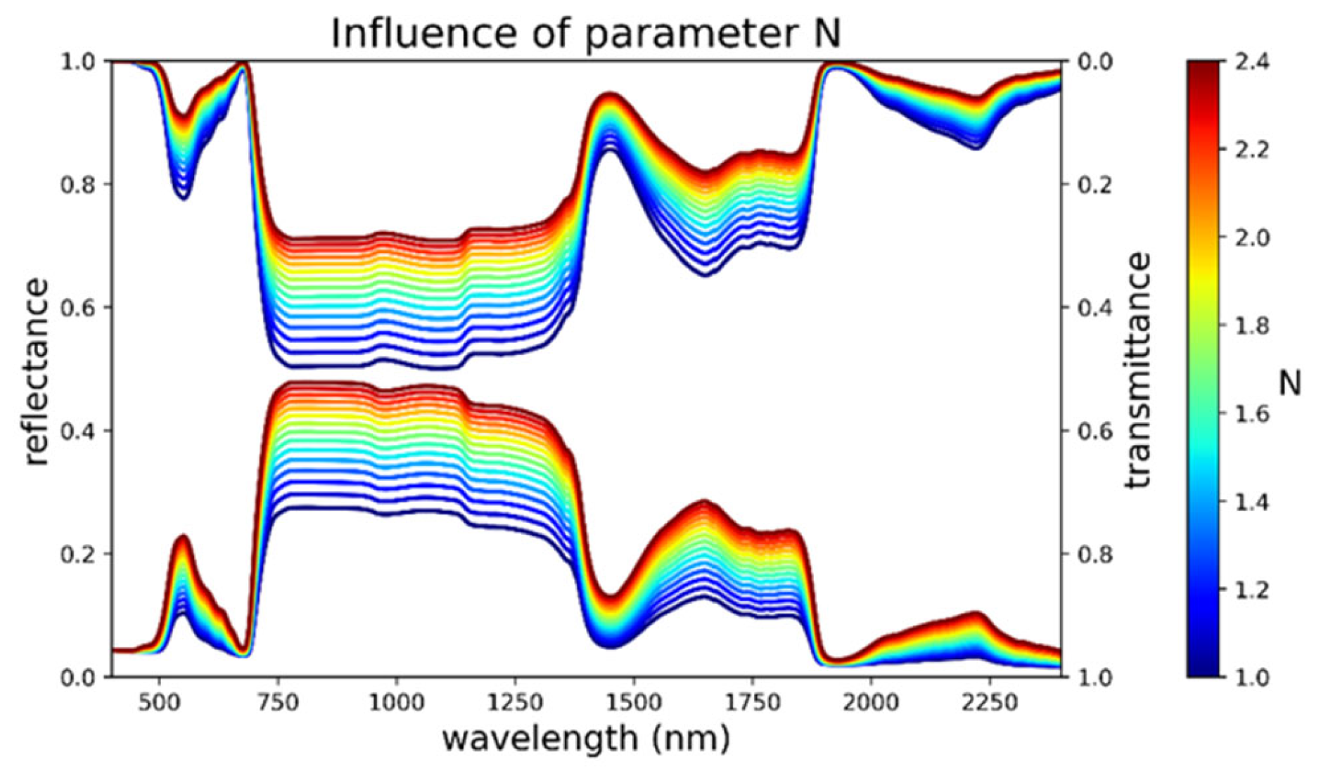
The parameter N has a major influence on LOPs simulated by the PROSPECT model since an increase in N tends to increase leaf reflectance and lower leaf transmittance. For example, Figure 4 highlights that a variation of 0.5 in N implies an increase in reflectance of 0.1 in the NIR region.
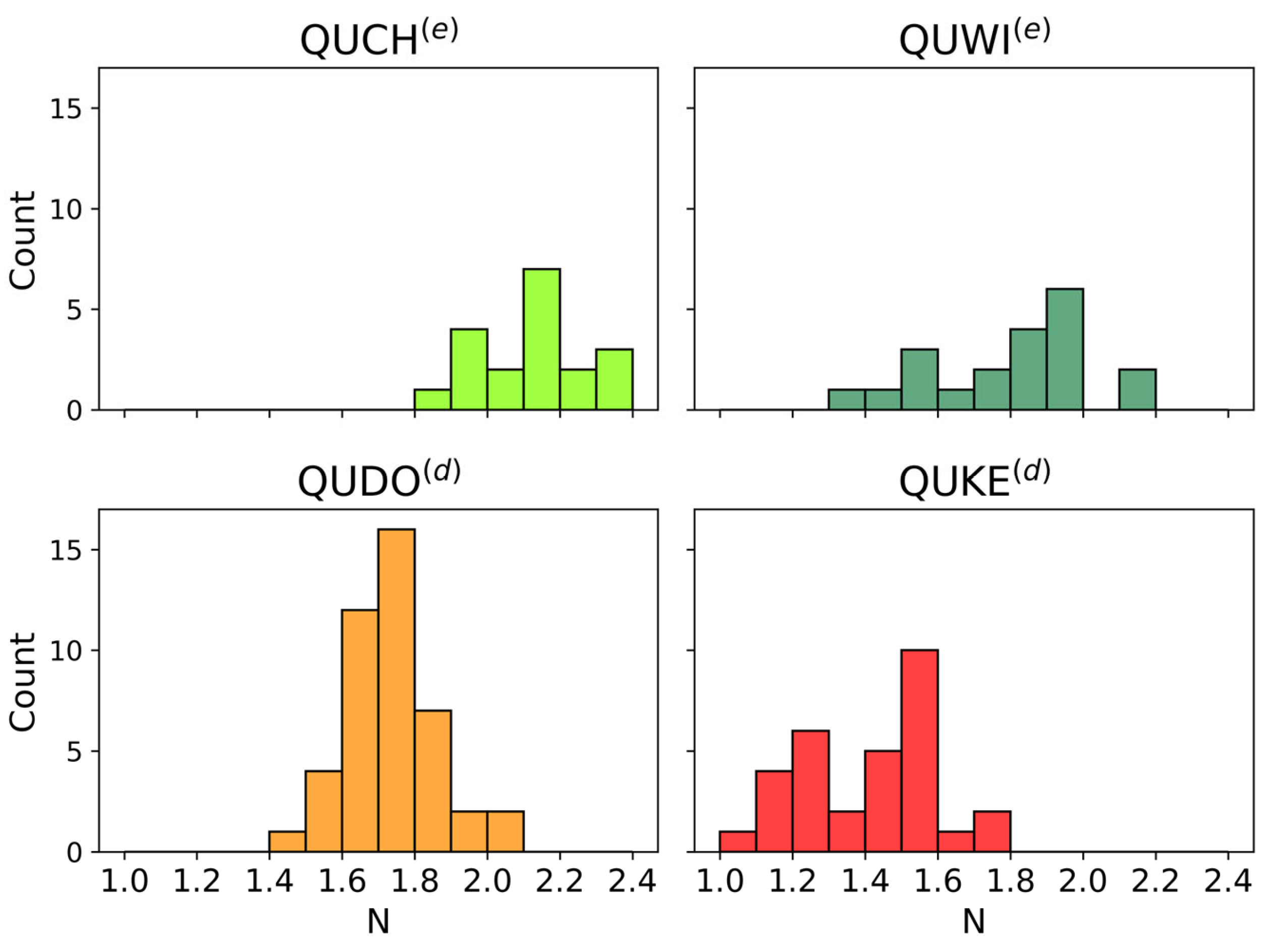
All estimated N values for each sample (i.e., tree) in the CSTARS dataset are within the range 1.0–2.4 (Figure 5). Globally, QUKE(d) has the lowest N median value while QUCH(e) has the highest N, with an absolute difference of 0.6. In comparison, QUDO(d) and QUWI(e) have comparable median values. The range of N values for QUKE(d) and QUWI(e) is 0.8, whereas it is 0.6 for QUDO(d) and QUCH(e). These results show the inter- and intraspecies variability in N can be larger than 0.5 and would be mirrored by the variability in LOPs. No site dependency is observed for N for the QUKE(d) and QUDO(d) species (Table 6).
For deciduous species, N has a seasonal influence since its value increases from spring to fall. But it is small for QUDO(d), with median N values from 1.67 in spring to 1.76 in the fall. In contrast, it is large for QUKE(d), with median variations from 1.22 to 1.60 (Figure 6). For evergreen species, no seasonal trend is clearly noticeable, mainly due to the lack of data in summer for QUCH(e) and spring for QUWI(e).
Estimated values of N are highly correlated with LMA (Pearson correlation coefficient equals 0.82; see Figure 7). For comparison, the three other leaf traits (Cab, Cxc, and EWT) show less correlation with estimated N (respectively, 0.39, 0.56, and 0.25). Moreover, estimated N is less correlated with leaf thickness (0.59) and leaf surface weight (sum of EWT and LMA; 0.69) than with LMA.

3.2. Leaf Trait Estimations

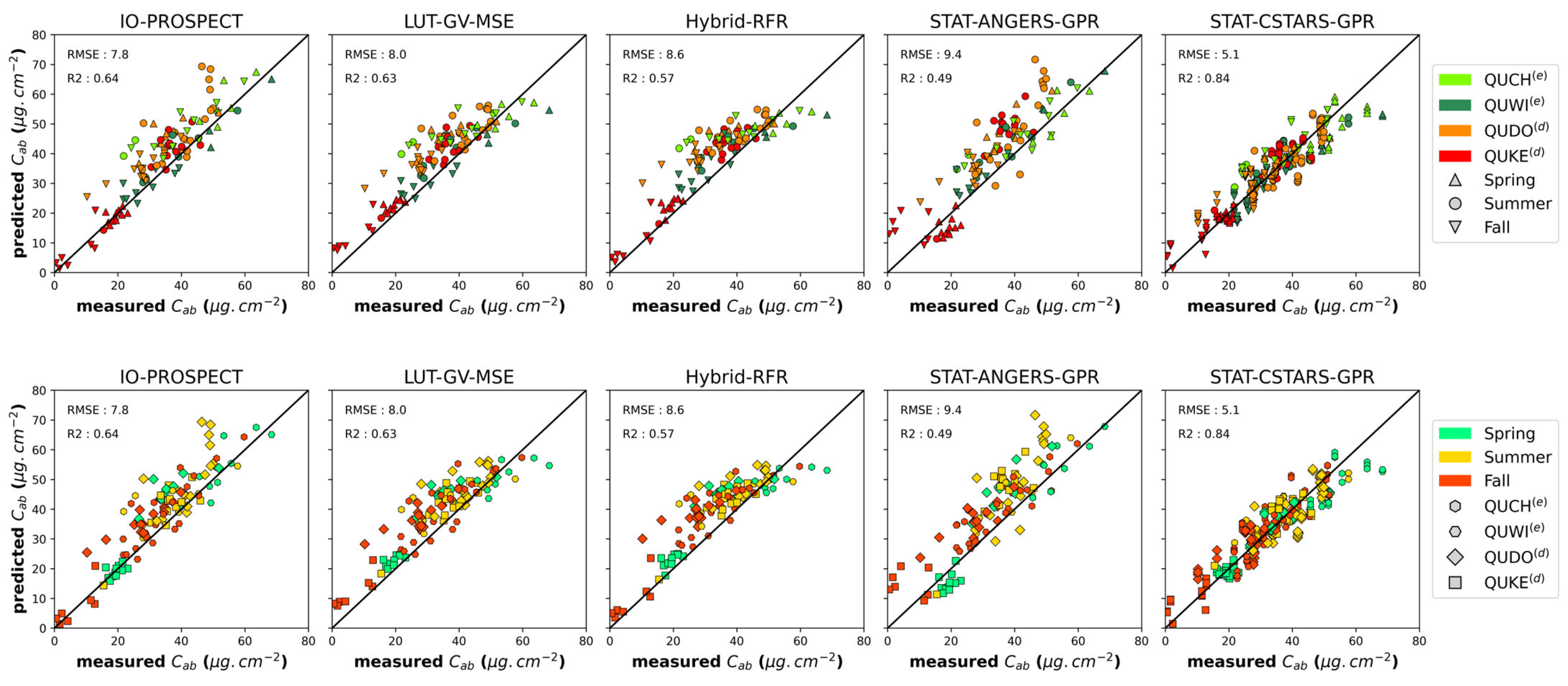
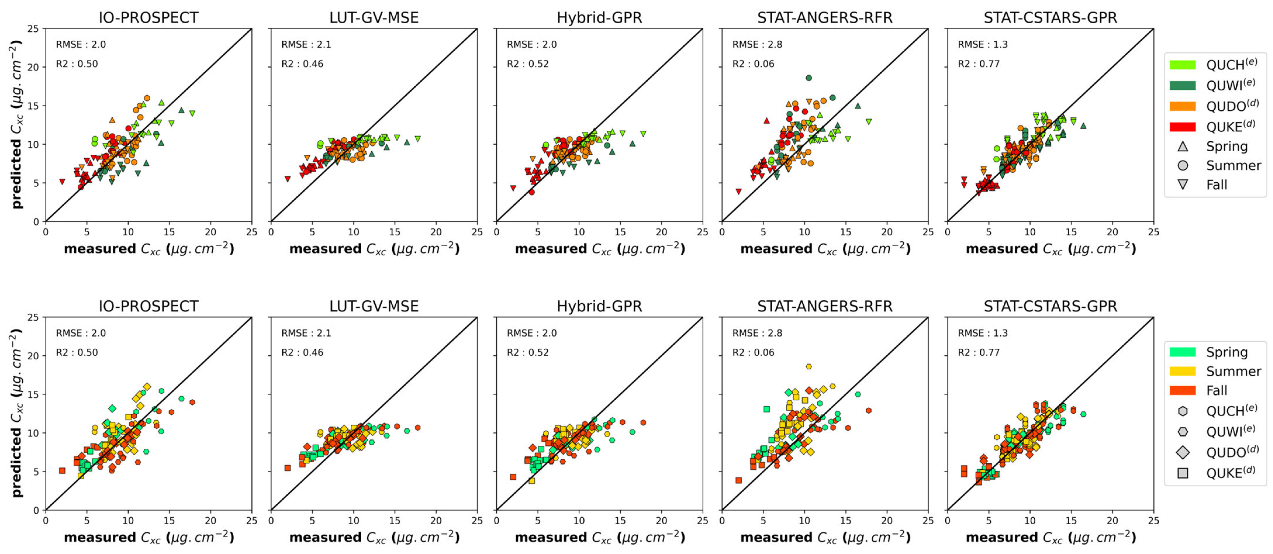
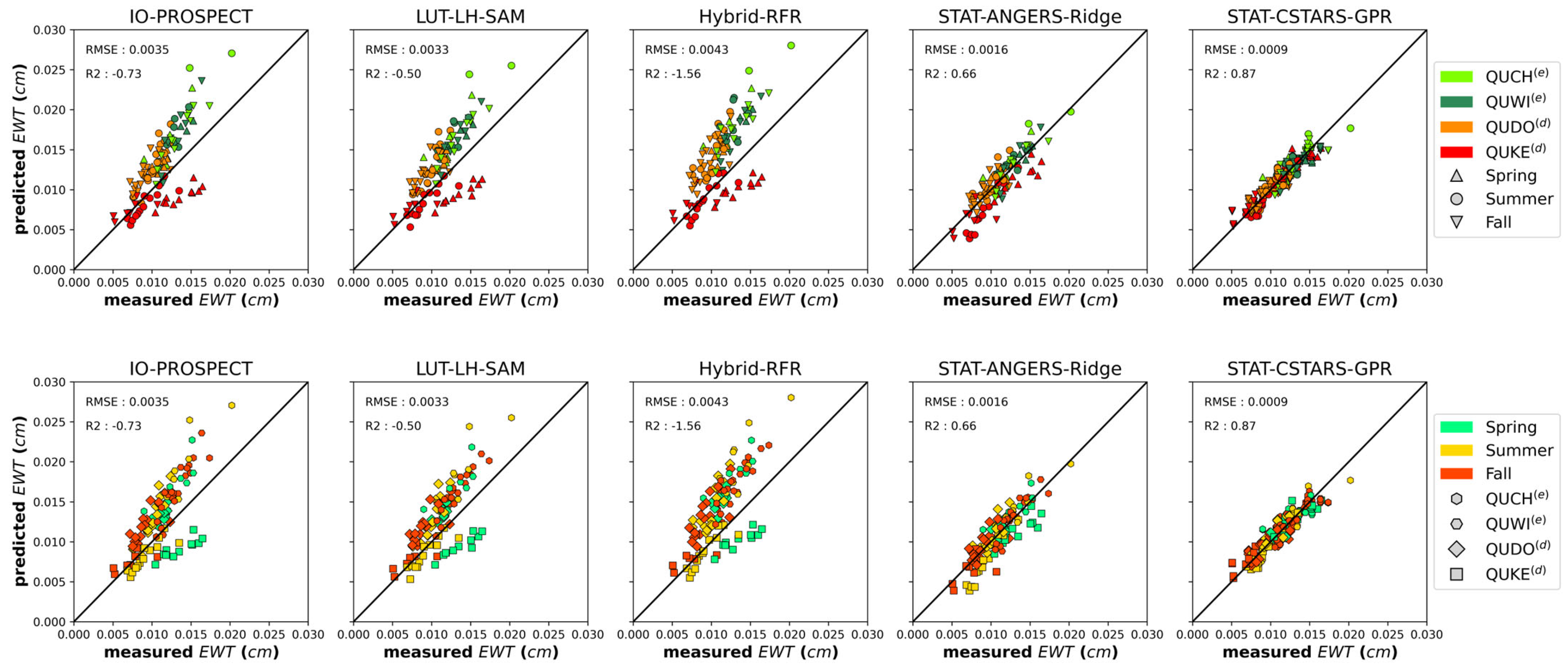
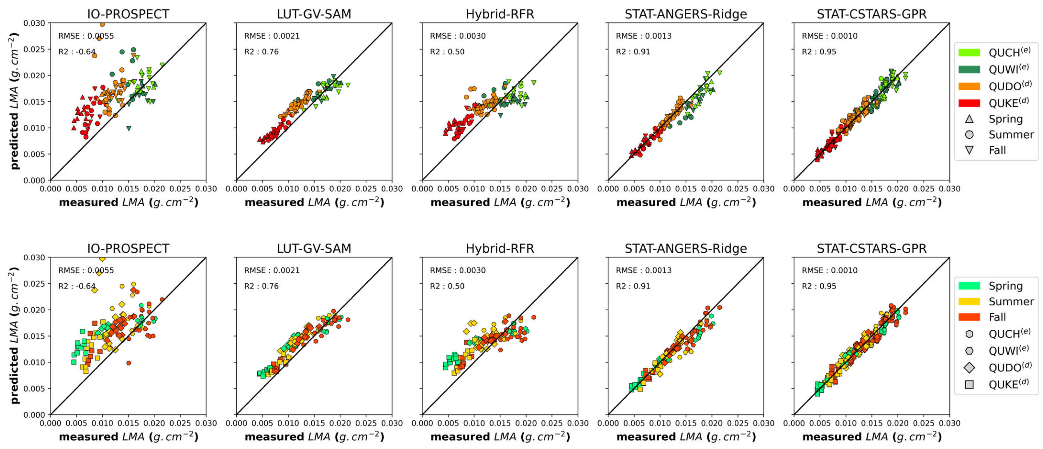
This section is divided into four subsections, each one describing the results for one leaf trait. For each leaf trait, all the accuracy metrics of all methods are compared for the whole CSTARS dataset. Detailed metric values by species and season are given for the two methods with the best accuracy (with the exception of Cxc due to comparable performance of two methods). Additionally, scatterplots compare estimates to measured leaf trait values for the most accurate method within each subcategory (cf. gray blocks in Figure 3). Two representations are chosen to display these scatterplots, the first by species and the second by season, in order to highlight potential specific or seasonal trends.

3.2.1. Chlorophyll Content

Higher accuracy was obtained for the STAT-CSTARS category, regardless of the chosen MLRA, with mean performance giving an RMSE equal to 5.7 µg/cm2, R2 around 0.77, and a bias under 0.3 µg/cm2 (Table 7). In this category, STAT-CSTARS-GPR yielded the most accurate estimates. For STAT methods, using the ANGERS dataset instead of CSTARS worsened RMSE performance by a factor of two on average.
For PROSPECT-based methods, IO-PROSPECT was the second best among all the methods considered, with bias still under 5.0 µg/cm2. LUT-based and hybrid inversions led to mitigating results. The accuracy of LUT-based methods was sensitive to the sampling strategy used to build the LUT (average RMSE for GV of 8.9 µg/cm2, average RMSE for LH of 14.5 µg/cm2). For hybrid methods, similar accuracy was obtained using non-linear methods (GPR, RFR) on the one hand and linear methods (PLSR, ridge) on the other, the former achieving better performance.
The influence of species and seasons on the results of the two most accurate methods (STAT-CSTARS and IO-PROSPECT) is analyzed in Table 8. For IO-PROSPECT, evergreen oaks (QUCH(e), QUWI(e)) deliver the best estimates whatever the season and have a low absolute bias (less than 2 µg/cm2). On the contrary, performance for deciduous oaks is inferior by a factor of two in terms of RMSE and has a significant bias. This plant functional type trend is not observed for STAT-CSTARS-GPR, which presents excellent biases whatever the species and season, under 2 µg/cm2 globally. Spring and fall have a better performance than summer for both methods. In general, QUDO(d) and QUCH(e) estimates are overestimated whatever the method, except for STAT-CSTARS (Figure 8). For fall and QUKE(d), particularly low Cab contents are observed and not correctly estimated (either over- or underestimated), except for IO-PROSPECT (Figure 8). This may highlight the limitations of PROSPECT in some cases and those of the training datasets (ANGERS, CSTARS) when dealing with extreme values.

3.2.2. Carotenoid Content

Same as Cab, STAT-CSTARS methods perform better than all other methods regardless of the chosen MLRA, with mean performances of RMSE = 1.4 µg/cm2, R2 around 0.71, and a bias under 0.1 µg/cm2 (Table 9). STAT-CSTARS-GPR yields the most accurate estimates for Cxc. Then, both IO-PROSPECT and non-linear hybrid methods provide the second most accurate results (RMSE around 2.0 µg/cm2, R2 around 0.5, bias around 0.5 µg/cm2). Like for Cab, non-linear hybrid methods perform better than linear ones. LUT-based inversions perform the worst (RMSE higher than 3.2 µg/cm2, GV still better than LH). STAT-ANGERS RMSE performance is inferior by a factor of more than 2 compared to STAT-CSTARS methods and by a factor of 1.5 compared to hybrid methods. Results are highly dependent on MLRA: they are better for non-linear methods (RMSE lower than 3.0 µg/cm2) than for linear ones (RMSE over 5.0 µg/cm2). Whatever the MLRA, estimates are biased (bias ranging from 1.5 to 5.1 µg/cm2).
Analyzing the three most accurate methods, STAT-CSTARS-GPR, HYBRID-GPR, and IO-PROSPECT, their species-dependent performance is less obvious in comparison with Cab (Table 10). On the one hand, when using HYBRID-GPR, there are more non-linear variations in Cxc estimates for evergreen oaks, with underestimations of Cxc above 13 µg/cm2 (Figure 9). A similar comment can be made for LUT-GV-MSE. On the other hand, STAT-CSTARS-GPR seems to have more homogeneous and robust variations whatever the species, which is indicated by R2 values between 0.5 and 0.7 while those of HYBRID-GPR are globally lower than 0.2 (Figure 9, Table 10). IO-PROSPECT behaves similarly to STAT-CSTARS-GPR, except that the absolute bias and RMSE are higher. Seasonally, HYBRID-GPR and IO-PROSPECT have similar performance. Taking into account R2 and bias, the three methods all had the worst results in summer.

3.2.3. Equivalent Water Thickness

Accurate estimates and excellent performance are obtained with STAT-CSTARS (RMSE < 0.0015 cm), without bias, while STAT-ANGERS is second best, also with a very low bias (<0.0007 cm in absolute values) except for when RFR is used (RMSE ≤ 0.0018 cm) (Table 11). Unexpectedly, for both STAT-ANGERS and STAT-CSTARS, GPR, ridge, and PLSR achieved quite similar results. Thus, it can be inferred that the relationship between spectral data and EWT is almost linear. IO-PROSPECT, LUT-based, and hybrid methods give RMSE estimations which are half as accurate as those provided by statistical methods (0.0033–0.0070 cm) and with higher biases (0.0018–0.0063 cm). Globally, IO-PROSPECT and LUT-based methods perform similarly for EWT. Hybrid methods delivered the highest biases.
The two best methods, STAT-CSTARS-GPR and STAT-ANGERS-Ridge, are further compared in Table 12. For STAT-CSTARS-GPR, RMSE is in the range 0.009–0.0015 cm, with a bias less than 0.0006 cm in absolute value. The highest RMSE is obtained for QUCH(e), and the highest bias is obtained for QUDO(d). One can note that the R2 of QUWI(e) is much lower (0.31). For STAT-ANGERS-Ridge, QUDO(d), QUCH(e), and QUWI(e) estimates have a similar RMSE (~0.0013 cm) with a bias less than 0.006 cm. In comparison, performance for QUKE(d) is inferior by almost a factor of two and with a larger bias (−0.0018 cm) when using the STAT-ANGERS-Ridge model. As such, non-specific species dependency is observed for the two methods. Then, considering each method by season, their RMSEs are similar and bias performance is low, with the spring season performing a bit worse.
All methods that rely on PROSPECT (physical and hybrid) seem to have a multiplicative bias whatever the species (Figure 10). The same trend is present for three species (QUCH, QUDO(d), and QUWI(e)), leading to an overestimation of EWT as EWT values increase. For QUKE(d) only, EWT is underestimated for values over 0.010 cm and under this threshold, EWT is accurately estimated. Notice that the cases with EWT over 0.010 cm are almost exclusively samples collected in spring. In contrast, statistical methods have almost no bias, which is more of an additive nature.

3.2.4. Dry Matter Content

Consistent with EWT estimations, STAT-CSTARS provides the most accurate estimates, followed by STAT-ANGERS with the use of GPR, PLSR, and ridge (RMSE = 0.0009 g/cm2, R2 = 0.95, and no bias for the former; mean RMSE = 0.0014 g/cm2, mean R2 = 0.9, and mean bias 0.0005 g/cm2 for the latter; Table 13). For STAT-ANGERS, PLSR and ridge have a lower RMSE, but PLSR is more reliable since it reduces the bias by a factor of two compared to ridge. The use of RFR leads to the lowest performances. For STAT-ANGERS, RMSE is increased by a factor of three and bias is five times greater than in the case of the other MLRAs. IO-PROSPECT, LUT-based, and hybrid methods yielded more biased estimations (bias is always higher than 0.0020 g·cm−2, except for hybrid-RFR, for which it was 0.0014 g/cm2) and lower accuracy than statistical methods (RMSE is around two times higher for the most accurate PROSPECT-based methods). For LUT-based methods, choosing SAM as a cost function instead of MSE improves accuracy (RMSE is reduced by a factor of two).
For deciduous species (QUDO(d) and QUKE(d)), both the STAT-CSTARS-GPR and STAT-ANGERS-Ridge methods showed similar performance, with better estimates than global RMSE (RMSE < 0.0009 g·cm−2; Table 14). In contrast, for evergreen species, the performance of STAT-CSTARS-GPR and STAT-ANGERS-Ridge is worse. Moreover, evergreen species exhibit poorer performance in terms of RMSE and R2. LMA for evergreen species is underestimated with STAT-ANGERS-Ridge (Figure 11) and estimates show a negative bias over 0.001 g·cm−2. No specific seasonal trend is noticed for both methods.
Globally, for statistical methods, linear MLRAs (ridge and PLSR) produce similar or better estimations than the two non-linear methods (GPR, RFR), and there are fewer significant differences between linear and non-linear methods with the use of the CSTARS dataset (STAT-CSTARS category).

4. Discussion

4.1. Variability in the PROSPECT Structure Parameter N

Considering the estimated N values, our study highlights the high interspecific and intraspecific variability in N. N has also a seasonal evolution in the four species of the same genus. Estimated global values of N range between 1 (minimum value for QUKE(d)) and 2.4 (maximum value for QUCH(e)), which is in line with previous studies. Indeed, Jacquemoud et al. [25] mentioned that, for dicotyledon leaves, N is usually in the range of 1.5–2.5 in experimental datasets and Spafford et al. [37] found a range of 1–2.5 for PROSPECT simulations in order to encompass a large variety of species. Below, variations in N are further discussed based on their interspecific variability (Section 4.1.1), intraspecific variability (Section 4.1.2), and influence on PROSPECT LOP simulations and leaf trait estimations (Section 4.1.3).

4.1.1. Interspecific Variability in N

In our results, intraspecific variations in N are noticeable. Evergreen oak species (QUWI(e) and QUCH(e)) exhibit higher N values than deciduous oaks regardless of the season. Particularly, QUKE(d) has a much lower mean N (1.42) compared to other species (1.74, 1.81, and 2.13 for QUDO(d), QUWI(e), and QUCH(e), respectively).
Analyzing the statistical link between N values and measurable parameters provides more interpretability of N variability. Indeed, the interspecific trend of N follows the interspecific trend of LMA exactly (2.1.3). This trend is confirmed by the high correlation between N and LMA (Pearson’s R = 0.82; Figure 7). While Demarez et al. [31] emphasized that N is correlated to leaf thickness, we found that N is less correlated to this latter parameter (Pearson’s R = 0.59) than to LMA. Moreover, compared to LMA, N shows less correlation to leaf surface weight (0.69) while this latter factor is more strongly linked to leaf thickness. Considering this, interspecific variations in N may be driven by LMA variations. And particularly, N being more correlated to LMA than to thickness means that N may be more related to the nature of leaf material than to its quantity.
The specificity of leaf surface, such as the presence of wax or a complex cuticle structure, is not simulated in the PROSPECT model. Therefore, we question whether the structural parameter N can compensate for effects due to cuticles and pubescence when modeling leaf reflectance. In our dataset, evergreen oaks QUWI(e) and QUCH(e) have a hard cuticle, leading to high specular reflection (as seen in Figure 1), and QUCH(e) leaves are pubescent on the abaxial side. QUDO has a quite hard leaf compared to QUKE(d), which is consistent with plant adaptation strategies for hot, low foothill habitats (i.e., woodland savannas). Considering these properties, N values might be higher for QUCH(e), QUWI(e), and QUDO(d) compared to QUKE(d) to compensate for their complex surface properties.

4.1.2. Intraspecific Variability in N

We also observe intraspecific variations in N. N dynamic range is 0.6 for QUCH(e) and QUDO(d) and reaches 0.8 for QUKE(d) and QUWI(e). Several factors can drive these intraspecific variations and are discussed hereafter.
The N parameter is expected to change over the course of the year following the phenological evolutions of a given species. Our dataset, collected at three different phenophases during the year, provides insight into this evolution. However, few studies actually provide information that can be compared with our results about N distribution for a given species and even less throughout a phenological cycle. Considering deciduous plants, phenological variations in N show an increase from spring to fall, as observed in forests [31,34] and crops [58]. For instance, Noda et al. [34] found that N ranges between 1 (from budburst in mid-May) and 1.4 (before leaf fall at the end of October) for leaves of Quercus Crispula. In our oak dataset, the same seasonal tendencies were observed for QUDO(d) (from 1.67 to 1.76) and QUKE(d) (from 1.22 to 1.60).
For evergreen species, QUCH(e) and QUWI(e), we found no particular seasonal trend for N with our dataset. However, during field sampling, priority was not given to evergreen species due to their smaller variations in leaf functional traits, and therefore we lack data throughout the year for QUCH(e) and QUWI(e) (respectively, in summer and spring). Moreover, for evergreen species, new leaves that grew in the years of sampling were not collected due to the assumption that previous years’ leaves make up the majority of the canopy. Therefore, during the leafing out period of evergreen oaks in spring, when one could expect the highest discrepancy compared to previous year’s generation, the new leaf generation was not sampled. This may explain why QUCH(e) and QUWI(e) show similar values of N and leaf traits in spring, summer, and fall. However, the two generations of leaves are less distinguishable in summer, and some new-generation leaves might have been collected in summer. This could explain why QUWI(e) N values are more variable for summer.
Jacquemoud et al. [22] provided a hypothesis to explain the increase in N from spring to fall, which was at least observed in deciduous species [31,34]. They stated that N estimated for dry leaves is higher than N estimated for fresh ones, probably due to an increase in multiple scattering due to the loss of water. However, our results show that N is strongly correlated to LMA. In addition, N exhibited almost no correlation with EWT and particularly leaves with lower N values could have high EWT values, around the average (e.g., QUKE(d) leaves in spring, see Figure 12). Therefore, N variations throughout the phenological cycle may be driven by the content of dry matter, which only increases during the leaf’s lifetime and may not be driven by water loss. Furthermore, other intraspecific variabilities in N that were observed might only be compelled by factors of LMA variation.
In addition, other sources of variations in the N parameter include leaf position within the highly heterogeneous vertical profile of the tree canopy and if the leaf developed in the shade or in the sun [31,34]. This could lead to a 5–10% rise in intraspecific variability [31]. In our dataset, it was sometimes impossible to collect leaves at the very top of the canopy, so for some of the 20 m and taller trees, leaves were collected from a part of the canopy that received less sunlight instead. Thus, this is another factor of N variation in our study that could have artificially increased intra- and interspecific variabilities in N.

4.1.3. Limitations of the PROSPECT Structure Parameter N and Its Impact on Leaf Trait Estimations

Generally, the N parameter has a substantial influence on the spectral shape of LOPs (cf. Figure 4). Ceccato et al. [59] conducted a sensitivity study showing that the N parameter can explain about 40% of the output. Thus, a precise estimation of N may therefore be required to accurately estimate leaf traits. In addition, assessing the performance of PROSPECT for leaf trait estimation at the extremes of the observed N values (close to 1 or 3) has not been explored; therefore, limitations of the PROSPECT model for these values remain partially unknown.
Spafford et al. [37] assessed the impact of retrieving the N value prior to estimating leaf traits with a method similar to IO-PROSPECT. They developed a correlation function between N and reflectance in the NIR band (wavelengths where pigments do not absorb) and used this correlation to accurately estimate the N parameter in isolation. Leaf traits were estimated with better accuracy than without the prior retrieval of the N value. However, their conclusion stated that with the knowledge of both leaf directional-hemispherical reflectance and transmittance, the use of optimized spectral subdomains yielded better accuracy without using the prior estimation of N. In our study, we did not use any previously estimated N value. Despite this fact, our results highlighted a large intraspecific variability in this parameter; therefore, one should not use a single previously estimated N value by species but rather estimate N each time, as in [37].
Moreover, Pacheco-Labrador et al. [60] found better estimations for the pigments and EWT of Quercus Ilex leaves with IO-PROSPECT by removing trichomes from the surfaces of the leaves. Their work indicates qualitatively that leaf surface impacts the leaf trait estimation accuracy of PROSPECT-based methods. In fact, the PROSPECT model does not simulate any specificity of leaf surface, while most plant leaves display a waxy surface or a complex cuticle structure. This shortcoming has been emphasized by several studies. Furthermore, for Cab estimation with PROSPECT, taking into account leaf surface reflection by adding an additional surface layer into the PROSPECT model or changing pigment-specific absorption coefficients demonstrated better performance, especially for leaves covered by heavy wax or hard cuticles [61,62]. But these results have barely been investigated for other leaf traits (i.e., Cxc, EWT, and LMA) and the concurrent impact of N values has not been studied to our knowledge.
In our dataset, QUWI(e) and QUCH(e) have a hard cuticle, leading to high specular reflection (as seen in Figure 1). In particular, QUCH(e) leaves are pubescent on the abaxial side. However, despite the fact that these features (presence of hairs, hard cuticle, asymmetry between adaxial and abaxial leaf surfaces) are not taken into account in the PROSPECT model, our estimations for all leaf traits are quite acceptable because they are globally only slightly poorer than those obtained for deciduous oaks (Figure 8, Figure 9, Figure 10 and Figure 11) by PROSPECT-based methods. Even though QUKE(d) possesses waxy leaf surfaces on the upper side (adaxial; as seen in Figure 1), QUKE(d) samples in spring exhibited low N values, between 1 and 1.4. In this range, a variation in N implies higher changes in simulated spectral variations in NIR and SWIR (Figure 4) where EWT is spectrally sensitive. These may be the two main reasons explaining the inaccurate estimations of EWT we obtained for QUKE(d) spring samples (see Figure 12 and Section 4.2 for further discussions on EWT estimation).

4.2. Comparison of Leaf Trait Estimation Methods

Estimation methods were tested for four leaf traits and to varying degrees, trends in the results are specific for each leaf trait. However, it is possible to identify trends common to all four leaf traits and to draw general conclusions; these are discussed below in Section 4.2.1. The specificity of results related to leaf pigment contents, EWT, and LMA are further discussed in Section 4.2.2, Section 4.2.3, and Section 4.2.4 respectively.

4.2.1. Estimation Method Considerations Common to All Four Variables

Globally, STAT-CSTARS methods showed greater accuracies, as expected, since the training and test data came from the same dataset which potentially included the same specific errors and bias. However, the four selected MLRAs yielded different estimation accuracies, with GPR providing the most accurate estimates for all the traits. Its performance is further used as a reference as it achieved the greatest retrieval performance in comparison with the other methods.
PROSPECT-based methods estimated leaf traits with less accuracy than STAT-CSTARS methods. Compared with STAT-ANGERS methods, the advantage of statistical methods is less clear, particularly for pigment content estimation. The transferability of statistical methods is further discussed in Section 4.3.
IO-PROSPECT was globally more accurate than the other PROSPECT-based methods. In our study, IO-PROSPECT presented limitations only in LMA estimation, which are discussed further in Section 4.2.4. For Cab, Cxc, and EWT, LUT-based and HYBRID methods yielded equally or less accurate estimates. Our assumption is that LUT-based and HYBRID methods are both built on synthetic datasets generated with PROSPECT and are therefore dependent on the sampling strategy used. This is particularly noticeable when comparing LUT-GV and LUT-LH used for the same trait. Conversely, IO-PROSPECT and other iterative inversions of PROSPECT use direct simulations with only the required parameter values. Moreover, LUT-based methods are difficult to calibrate since they involve three main parameters (sampling scheme, distance function, and q ) whose effects remain unclear. For example, the optimal q was selected from our dataset, but this could be considered overfitting, and the results we obtained with LUT-based methods should be considered less reliable. In addition, LUT-based methods are not clearly more efficient than IO-PROSPECT, particularly when using a LUT with many samples. Thus, we consider that iterative inversions of PROSPECT should be chosen over LUT-based methods. HYBRID methods build estimators from an MLRA and a synthetic dataset. They can overfit on synthetic data and become less resilient to noise or other spectral measurements errors.
In our study, for both statistical and hybrid methods, we compared estimators built with four MLRAs: ridge, PLSR, GPR, RFR. However, it may not be possible to draw an unambiguous conclusion regarding the most appropriate choice of MLRA. For statistical methods, Yang et al. [63] compared different MLRAs trained on leaf reflectance only (SVR, PLSR, RFR and K-Nearest Neighbors) for the estimation of EWT and LMA. Overall, their results show that EWT was more accurately estimated with SVR. For LMA, results were not unequivocal and mostly depended on the training dataset. In contrast, for EWT and LMA, we obtained an accurate estimation with linear MLRAs (ridge and PLSR), highlighting that the relationship between LOPs and EWT/LMA is approximately linear. These two MLRAs were followed by GPR. GPR also provided good results for Cab and Cxc (only RFR stayed one step ahead for Cxc). While choosing an MLRA for statistical methods, GPR may be the best compromise, since it is more versatile and able to deal with linear and non-linear problems. For hybrid methods, RFR obtained the best accuracy for Cab, EWT, and LMA and a very good accuracy for Cxc compared to other MLRAs. Therefore, RFR may provide more robust estimators to cope with the transition from synthetic data to measured data.
Each method includes numerous parameters that could be optimized. However, the idea of our study is to investigate a wide range of methods; therefore, we choose to optimize only major parameters which were always considered in previous studies. In contrast, some studies specifically tackled the optimization of other parameters whose effects are not evaluated in our work. Firstly, defining a trait-specific spectral range is a thorny question for all estimation methods. Some previous studies tackle this issue and search for optimal ranges of several leaf traits. But these investigations focus on iterative inversions of PROSPECT, such as those developed by Féret et al. [29] or Spafford et al. [37], who found optimized spectral subdomains for the four leaf traits (Cab: 0.7–0.72 µm, Cxc: 0.52–0.56 µm, and EWT/LMA: 1.7–2.4 µm). It is not clear if using these spectral subdomains for statistical or hybrid methods would yield more accurate estimates. In our study, we used the same spectral ranges for statistical, hybrid, and LUT-based methods (Cab: 0.45–0.76 µm, Cxc: 0.45–0.56 µm, EWT: 0.9–2.4 µm, and LMA: 0.75–2.4 µm) and they were built on sensitivity analysis results. These ranges differ from the optimal ranges found for iterative inversions of PROSPECT [29,37]. They also differ from those already used at the canopy level for oaks (Cab: 0.5–0.75 µm and Cxc: 0.5–0.55 µm with a LUT-based method [64]; EWT/LMA: 1.5–2.4 µm with hybrid PLSR [24]). Nevertheless, despite potential for future improvements, good performance was obtained for each leaf trait of these four oak species.
Moreover, transformations of spectral data could be used in statistical and hybrid methods to extract features or reduce their number for MLRA inputs. Particularly, Yang et al. [63] compared statistical methods based on reflectance or spectral indices. They found that estimation accuracy was improved (reduced by 5.7%) when using spectral indices rather than reflectance. However, all our tested approaches were LOP-based and we did not apply transformations such as spectral indices or dimensionality reductions.

4.2.2. Estimation of Leaf Pigments

For leaf pigments, IO-PROSPECT was the best method after STAT-CSTARS-GPR with a higher accuracy for Cab (RMSE of 7.8 and 5.0 µg·cm−2, respectively) than for Cxc (2.0 and 1.3 µg·cm−2). In particular, STAT-CSTARS-GPR estimates had a very low bias for both pigments (both 0.1 µg·cm−2) compared to IO-PROSPECT (4.9/0.4 µg·cm−2 for Cab/Cxc). Generally, in the literature, IO-PROSPECT is the most widely used inversion method [26,30,31,62]. For Cab, the results are in the same order of magnitude when compared to other studies. Demarez et al. [31] found an RMSE of 7.3 µg·cm−2 over phenological variations of oaks, beeches, and hornbeams. They had a bias that increased with crown leaf position: from 2 µg·cm−2 for sunlit leaves to 19 µg·cm−2 for shaded leaves for oaks. In comparison, we obtained a bias of 4.9 µg·cm−2. Qiu et al. [62] obtained an RMSE of 8.9 µg·cm−2 for broadleaf leaf samples by accounting for leaf surface reflection. Wang et al. [30] produced an RMSE of 13.1 and 10.9 µg·cm−2 for two large datasets including trees, shrubs, and grass from USA and China and from temperate to tropical climates. Féret et al. [26] reported an RMSE of 9.0 µg·cm−2 among several available datasets and [32] provided an RMSE of 6.3 µg·cm−2 for a temperate forest with vertical variability within the canopy. For Cxc, our results are also in line with previous studies ([26]: RMSE = 3 µg·cm−2; [30]: RMSE = 3.5/5.3 µg·cm−2).
Then, evaluating seasonal variations in estimation performance for Cab, Gara et al. [32], using a LUT-based method, noticed that the lowest accuracy corresponds to the summer period when they pooled all leaf samples collected from the upper canopy (spring/summer/fall: RMSE = 7.1/7.3/5.8 µg·cm−2). The same tendency occurred in our dataset (spring/summer/fall: RMSE = 7.0/9.2/7.0 µg·cm−2) and was also reported by Zhang et al. [65]. This can possibly be explained by a reorganization of the chloroplast (which contains the pigments) in the leaf cytoplasm from being clumped during peak vegetative growth to being more uniformly distributed when leaves start being senescent [32]. However, we also found that a statistical method such as PLSR [66] produced better estimations for summer than other seasons. For Cxc, we did not find a particular seasonal trend compared to Cab (spring/summer/fall: RMSE = 2.2/2.0/1.9 µg·cm−2). To our knowledge, no study exists in the literature with which to compare our findings for Cxc. Differentiating by species and plant functional types, we observed better results for evergreen species for Cab (RMSE twice lower, R2 very significantly higher, low biases) but the opposite was found for Cxc to a lesser extent (higher RMSE and R2, similar biases).
At the canopy level, using the same dataset as ours combined with AVIRIS airborne hyperspectral images, Miraglio et al. [24,64] found that leaf pigments were correctly estimated with a LUT-based method for QUDO(e) at the TONZ site (Cab: RMSE = 5.2 µg·cm−2; Cxc: RMSE = 1.34 µg·cm−2) and with a statistical method for QUDO(d) and QUWI(e) at both the TONZ and SJER sites (Cab: RMSE ≈ 7.91 µg·cm−2; Cxc: RMSE ≈ 1.73 µg·cm−2). This demonstrates that our results have potential for upscaling from the leaf to canopy level for oak woodland savannas. But in contrast to the leaf level, canopy estimations for Cab during summer periods did not produce particularly worse results than those made for fall samples [64].

4.2.3. Estimation of Leaf Water Content

For EWT, statistical methods yielded more accurate estimates than PROSPECT-based methods. RMSE was reduced by 50% with STAT-ANGERS-Ridge compared to IO-PROSPECT or LUT-LH-SAM. On the other hand, Féret et al. [29] reached the opposite conclusion and showed that PROSPECT inversions could outperform statistics-based methods (using SVM as the MLRA) using an optimized spectral subdomain (1700 to 2400 nm).
PROSPECT inversions for EWT estimation lead to an RMSE of 0.0035 cm, which is similar to that obtained by Asner et al. [35] for heterogeneous humid tropical forests using an 800–2400 nm spectral range. However, regardless of the PROSPECT-based method, our estimates exhibit two major deficient trends: a multiplicative bias and underestimation for some QUKE(d) samples.
Firstly, EWT is estimated with multiplicative bias, which is particularly noticeable for QUDO(d), QUWI(e), and QUCH(e) samples, which have higher EWT. While such multiplicative bias was not systematically reported by previous studies, one can find some hints of such bias in the work of Gara et al. [32]. Indeed, using a LUT-based method, Gara et al. [32] found that higher values of EWT were overestimated, which reveals a similar multiplicative bias. However, EWT values in Gara et al. [32] only reach 0.012 cm; therefore, the bias is less noticeable than in our experiment, where some EWT values are over 0.015 cm. Similarly, a multiplicative bias was found by Pacheco-Labracor et al. [60] for IO-PROSPECT, which in their study tended to underestimate EWT. This bias was attenuated by removing leaf trichomes from Quercus Ilex prior to spectral measurement. Conversely, Wang et al. [30] did not find the same tendency in large datasets using PROSPECT iterative inversion and they obtained unbiased estimates of EWT with high accuracy (R2 = 0.74/0.77, RMSE = 0.0022/0.0036). Different sources of errors could explain the bias observed in our results when using PROSPECT. On the one hand, the Quercus species present in our sites are not considered in the calibration databases used to set some parameters of PROSPECT-D (surface scattering, unique value of refractive index, etc.). On the other hand, some bias could exist in the leaf optical measurements [29].
Secondly, EWT is underestimated for some samples. These latter samples originate from QUKE(d) oaks, almost exclusively from spring 2014 collections. Inaccurate estimations for QUKE(d) in spring can have multiple sources of origin. (i) Most of the samples that exhibit an underestimation of EWT were collected at the BLOF site in the 2014 spring campaign. Measurements from this campaign could have been biased. (ii) QUKE(d) leaves are larger compared to those of the other species, which may have led to a poor representativeness of LOPs when considering the whole leaf area. Lastly, (iii) these samples also exhibited low N values (Figure 12). This range of values for N has not been fully studied, and in this range, N has more impact in NIR and SWIR (Figure 4) where EWT is spectrally sensitive.
However, both issues (multiplicative bias and underestimation for QUKE(d) spring samples with low N) are not observed in estimates from statistics-based methods, including STAT-ANGERS methods (see Figure 12). This may also indicate that these estimation issues come from inaccurate modeling of PROSPECT for oak EWT and suggest that PROSPECT is not fully suited for our dataset.

4.2.4. Estimation of Leaf Dry Matter Content

Estimating LMA using PROSPECT, Asner et al. [35] found similar orders of magnitude as in our results (0.0033 g·cm−2), although the forest types in their study are very different. Nevertheless, our statistical methods, including STAT-ANGERS methods, outperform PROSPECT-based methods. Similar to EWT, this leads to opposite conclusions than those made by Féret et al. [29]. However, results obtained with IO-PROSPECT are surprising since this method yielded equally or more accurate estimates than other PROSPECT-based methods for the other three leaf traits. In the case of LMA, LUT-based methods provided more accurate estimates. Particularly, using SAM as the distance function for LUT-based methods led to better result; with MSE, this difference was not as noticeable for other leaf traits. Considering hybrid methods, using RFR as the MLRA yielded more accurate estimates. Indeed, the difference between RFR and other MLRAs was more pronounced for LMA than for other leaf traits.
Generally, our estimation results showed global overestimations of LMA using PROSPECT-based methods (bias over 0.0014 g·cm−2) while statistical methods showed lower bias. Gara et al. [32] found underestimations regardless of the season. They found no particular seasonal trend in their dataset (spring/summer/fall: R2 = 0.67/0.82/0.78, RMSE = 0.0014/0.0013/0.0014 g·cm−2; global: R2 = 0.76, RMSE = 0.0014 g·cm−2). More particularly for evergreen oaks, Gonzáles-Cascón et al. [38] estimated the LMA of Quercus Ilex leaves with high performance (R2 = 0.90) by using a PLSR statistical method. For comparison, for QUCH and QUWI, we obtained a mean R2 of 0.62 and RMSE of 0.0012 g·cm−2 with STAT-CSTARS-GPR.

4.3. Transferability of Statistical Methods Trained on an Independent Dataset

Considering the transferability of statistical methods, similar trends are observed for all leaf traits when comparing STAT-ANGERS to STAT-CSTARS. The lowest RMSE obtained with STAT-ANGERS methods is around twice the value obtained by STAT-CSTARS-GPR for Cab, Cxc, and EWT. For LMA, the difference is less important: the RMSE obtained with STAT-ANGERS-Ridge is around 1.3 times the size of the RMSE obtained with STAT-CSTARS-Ridge. The same trend is observed in the work of Wang et al. [30]. They evaluated the transferability of a PLSR statistical method to retrieve foliar traits across two datasets collected in a tropical and subtropical forest in China and a temperate and subtropical forest in the United States. Wang et al. demonstrated that their PLSR-based method yielded a lower accuracy when applied to an independent dataset, unused in training data. Similarly to our results, they found that a lower relative RMSE difference was reached for LMA (around 35%).
Féret et al. [29] and Yang et al. [30] evaluated the transferability of statistics-based methods for EWT and LMA. They performed a cross-dataset validation using two independent training and test datasets. They showed that the results are highly dependent on both the training and test datasets. Moreover, Féret et al. (2019) demonstrated that combining several datasets for training in order to increase the size of the training set improves the results. Consequently, the order of magnitude we found when comparing the RMSE obtained with STAT-CSTARS and STAT-ANGERS depends on our datasets, and it is very likely that different RMSE variations would be observed using other datasets.
Both Féret et al. [29] and Wang et al. [30] also compared statistical methods to PROSPECT-based methods similar to our IO-PROSPECT. Wang et al. [30] estimated the same four leaf traits as in our study, while Féret et al. focused on EWT and LMA. In the work of Wang et al., the transferred PLSR-based method achieved better accuracy than their equivalent to our IO-PROSPECT method for LMA and Cxc. Féret et al. obtained better accuracy for LMA with statistical methods for half of the cases they studied, but these results were highly dependent on the datasets used for training and testing. These results are in line with the accuracy we obtained for LMA. However, both studies reached better accuracy with improved versions of IO-PROSPECT and demonstrated that our IO-PROSPECT method is not perfectly suited for the estimation of EWT and LMA. Therefore, the opposite conclusions could be drawn if we modified the IO-PROSPECT method.

5. Conclusions

This work aimed to compare several statistical, physical, and hybrid estimation methods for four foliar traits of leaves of California oak species collected from four sites in three different seasons.
We showed that the structural parameter N in PROSPECT depends little on the season for evergreen species, which was not the case for deciduous species. Our estimation methods had no prior knowledge of the N parameter, although trait estimates were obtained with good accuracy.
In conclusion, the most accurate estimation methods for all leaf traits are statistical methods built on a dataset that include the same species composition and are measured with the same protocol. Among the four MLRAs tested, GPR enabled the development of the most accurate estimator (i.e., STAT-CSTARS-GPR). However, we noticed that statistical linear methods deliver better results for EWT and LMA. On the contrary, non-linear ones are better for leaf pigments. However, deriving such data is very demanding in terms of time and resources (for instance, to account for seasonality and geographic sampling) and requires high laboratory measurement costs (e.g., for pigments).
Other than that, physical inversion methods yield more accurate estimates for leaf pigment contents. Indeed, this class of methods delivers a similar performance. We recommend using IO-PROSPECT for pigments and EWT because it estimates these traits with good accuracy and performs a joint estimation of the leaf traits. For LMA, HYBRID-RFR is the most powerful method.
We used our dataset to evaluate the transferability of statistical methods trained on an independent dataset (ANGERS). For EWT and LMA, we demonstrated that this type of statistical methods leads to better estimation accuracy than PROSPECT-based methods. Particularly, statistical methods using linear models (STAT-ANGERS-PLSR or -Ridge) provided more accurate estimates. The performance of STAT-ANGERS methods was inferior compared to physical methods for pigments. In particular, results for Cxc were inferior by 50%, but for Cab, this occurred to a lesser extent. Therefore, we emphasize that statistical methods are promising estimation methods and a better understanding of their functioning could improve their transferability.
Considering the impact of seasons on each trait and its associated most accurate estimation method, estimation errors in terms of RMSE were similar. Estimation performance did not depend particularly on species but on plant functional type (evergreen or deciduous).
Finally, trait estimates were obtained from spectra averaged over several leaves and compared to the mean biochemical composition of this set of leaves. This constitutes an intermediary scale between the single-leaf and the canopy scales. Thus, this work provides insights into the upscaling of leaf trait estimation at the canopy level using imaging spectroscopy.

Author Contributions

Conceptualization, T.G., K.A., S.U. and X.B.; methodology, T.G.; software, T.G.; validation, T.G.; formal analysis, T.G.; investigation, T.G.; resources, M.H., K.A. and S.U.; data curation, T.G. and M.H.; writing—original draft preparation, T.G., K.A., M.H. and X.B.; writing—review and editing, T.G., K.A., M.H., S.U. and X.B.; visualization, T.G.; supervision, S.U. and X.B.; project administration, S.U. and X.B.; funding acquisition, K.A., S.U. and X.B. All authors have read and agreed to the published version of the manuscript.

Funding

This work was funded by CNES (Centre National d’Études Spatiales), Région Occitanie, and by ONERA (Office National d’Études et de Recherches Aerospatiales).

Data Availability Statement

Restrictions apply to the availability of these data. Data was obtained from CSTARS, University of California, Davis, and are available from the author with the permission of CSTARS, University of California, Davis.

Acknowledgments

The authors are grateful to the CSTARS team (University of California, Davis) for collecting and processing the field data as part of the HyspIRI Preparatory Science Campaign (S.L. Ustin PI, NASA grant #NNX12AP87G, “Identification of Plant Functional Types by Characterization of Canopy Chemistry”).

Conflicts of Interest

The authors declare no conflict of interest.

References

  1. Carrero, C.; Jerome, D.; Beckman, E.; Byrne, A.; Coombes, A.J.; Deng, M.; Rodríguez, A.G.; Van Sam, H.; Khoo, E.; Nguyen, N.; et al. The Red List of Oaks 2020; The Morton Arboretum: Lisle, IL, USA, 2020. [Google Scholar]
  2. Stavi, I.; Thevs, N.; Welp, M.; Zdruli, P. Provisioning Ecosystem Services Related with Oak (Quercus) Systems: A Review of Challenges and Opportunities. Agrofor. Syst. 2022, 96, 293–313. [Google Scholar] [CrossRef]
  3. Nixon, K.C. The Oak (Quercus) Biodiversity of California and Adjacent Regions; USDA Forest Service General Technical Report PSW-GTR-184; USDA Forest Service: Washington, DC, USA, 2002; pp. 3–20. [Google Scholar]
  4. Gaman, T. California’s Oaks in the 21st Century: Mapping Oak Woodlands and Forests. californiaoaks.org 2022. Available online: https://californiaoaks.com (accessed on 1 September 2023).
  5. Gaman, T.; Firman, J. Oaks 2040: The Status and Future of Oaks in California; California Oak Foundation: Oakland, CA, USA, 2006. [Google Scholar]
  6. Dib, T.; Ait Said, S.; Krouchi, F. Monitoring Long-Term Cork Oak Forest Spatio-Temporal Dynamics Based on Aerial Photographs: A Case Study of Kiadi Corks Oak Forest in Akfadou Mountain (Algeria). Analele Univ. Din Oradea Ser. Geogr. 2022, 32, 26–38. [Google Scholar] [CrossRef]
  7. Meng, R.; Wu, J.; Zhao, F.; Cook, B.D.; Hanavan, R.P.; Serbin, S.P. Measuring Short-Term Post-Fire Forest Recovery across a Burn Severity Gradient in a Mixed Pine-Oak Forest Using Multi-Sensor Remote Sensing Techniques. Remote Sens. Environ. 2018, 210, 282–296. [Google Scholar] [CrossRef]
  8. Carreiras, J.M.B.; Pereira, J.M.C.; Pereira, J.S. Estimation of Tree Canopy Cover in Evergreen Oak Woodlands Using Remote Sensing. For. Ecol. Manag. 2006, 223, 45–53. [Google Scholar] [CrossRef]
  9. Yousefi, S.; Haghighian, F.; Naghdyzadegan Jahromi, M.; Pourghasemi, H.R. Chapter 26—Pest-Infected Oak Trees Identify Using Remote Sensing-Based Classification Algorithms. In Computers in Earth and Environmental Sciences; Pourghasemi, H.R., Ed.; Elsevier: Amsterdam, The Netherlands, 2022; pp. 363–376. ISBN 978-0-323-89861-4. [Google Scholar]
  10. Kattenborn, T.; Schmidtlein, S. Radiative Transfer Modelling Reveals Why Canopy Reflectance Follows Function. Sci. Rep. 2019, 9, 6541. [Google Scholar] [CrossRef] [PubMed]
  11. Violle, C.; Navas, M.-L.; Vile, D.; Kazakou, E.; Fortunel, C.; Hummel, I.; Garnier, E. Let the Concept of Trait Be Functional! Oikos 2007, 116, 882–892. [Google Scholar] [CrossRef]
  12. Lausch, A.; Erasmi, S.; King, D.J.; Magdon, P.; Heurich, M. Understanding Forest Health with Remote Sensing -Part I—A Review of Spectral Traits, Processes and Remote-Sensing Characteristics. Remote Sens. 2016, 8, 1029. [Google Scholar] [CrossRef]
  13. Croft, H.; Chen, J.M.; Wang, R.; Mo, G.; Luo, S.; Luo, X.; He, L.; Gonsamo, A.; Arabian, J.; Zhang, Y.; et al. The Global Distribution of Leaf Chlorophyll Content. Remote Sens. Environ. 2020, 236, 111479. [Google Scholar] [CrossRef]
  14. Pereira, H.M.; Ferrier, S.; Walters, M.; Geller, G.N.; Jongman, R.H.G.; Scholes, R.J.; Bruford, M.W.; Brummitt, N.; Butchart, S.H.M.; Cardoso, A.C.; et al. Essential Biodiversity Variables. Science 2013, 339, 277–278. [Google Scholar] [CrossRef]
  15. Gamon, J.A.; Qiu, H.-L.; Sanchez-Azofeifa, A. Ecological Applications of Remote Sensing at Multiple Scales. In Functional Plant Ecology; CRC Press: Boca Raton, FL, USA, 2007; pp. 655–684. [Google Scholar]
  16. Ustin, S.; Asner, G.; Gamon, J.; Huemmrich, K.; Jacquemoud, S.; Schaepman, M.; Zarco-Tejada, P. Retrieval of Quantitative and Qualitative Information about Plant Pigment Systems from High Resolution Spectroscopy. In Proceedings of the 2006 IEEE International Symposium on Geoscience and Remote Sensing, Denver, CO, USA, 31 July–4 August 2006; pp. 1996–1999. [Google Scholar]
  17. Colombo, R.; Busetto, L.; Meroni, M.; Rossini, M.; Panigada, C. Optical Remote Sensing of Vegetation Water Content. In Hyperspectral Indices and Image Classifications for Agriculture and Vegetation; CRC Press: Boca Raton, FL, USA, 2018; ISBN 978-1-315-15933-1. [Google Scholar]
  18. Féret, J.-B.; Berger, K.; de Boissieu, F.; Malenovský, Z. PROSPECT-PRO for Estimating Content of Nitrogen-Containing Leaf Proteins and Other Carbon-Based Constituents. Remote Sens. Environ. 2021, 252, 112173. [Google Scholar] [CrossRef]
  19. Gara, T.W.; Rahimzadeh-Bajgiran, P.; Darvishzadeh, R. Forest Leaf Mass per Area (LMA) through the Eye of Optical Remote Sensing: A Review and Future Outlook. Remote Sens. 2021, 13, 3352. [Google Scholar] [CrossRef]
  20. Jacquemoud, S.; Ustin, S. Leaf Optical Properties; Cambridge University Press: Cambridge, UK, 2019. [Google Scholar]
  21. Verrelst, J.; Malenovský, Z.; Van der Tol, C.; Camps-Valls, G.; Gastellu-Etchegorry, J.-P.; Lewis, P.; North, P.; Moreno, J. Quantifying Vegetation Biophysical Variables from Imaging Spectroscopy Data: A Review on Retrieval Methods. Surv. Geophys. 2019, 40, 589–629. [Google Scholar] [CrossRef] [PubMed]
  22. Jacquemoud, S.; Ustin, S.L.; Verdebout, J.; Schmuck, G.; Andreoli, G.; Hosgood, B. Estimating Leaf Biochemistry Using the PROSPECT Leaf Optical Properties Model. Remote Sens. Environ. 1996, 56, 194–202. [Google Scholar] [CrossRef]
  23. Ali, A.M.; Darvishzadeh, R.; Skidmore, A.K.; Duren, I.V.; Heiden, U.; Heurich, M. Estimating Leaf Functional Traits by Inversion of PROSPECT: Assessing Leaf Dry Matter Content and Specific Leaf Area in Mixed Mountainous Forest. Int. J. Appl. Earth Obs. Geoinf. 2016, 45, 66–76. [Google Scholar] [CrossRef]
  24. Miraglio, T.; Adeline, K.; Huesca, M.; Ustin, S.; Briottet, X. Assessing Vegetation Traits Estimates Accuracies from the Future SBG and Biodiversity Hyperspectral Missions over Two Mediterranean Forests. Int. J. Remote Sens. 2022, 43, 3537–3562. [Google Scholar] [CrossRef]
  25. Jacquemoud, S.; Baret, F. PROSPECT: A Model of Leaf Optical Properties Spectra. Remote Sens. Environ. 1990, 34, 75–91. [Google Scholar] [CrossRef]
  26. Féret, J.-B.; François, C.; Asner, G.P.; Gitelson, A.A.; Martin, R.E.; Bidel, L.P.R.; Ustin, S.L.; le Maire, G.; Jacquemoud, S. PROSPECT-4 and 5: Advances in the Leaf Optical Properties Model Separating Photosynthetic Pigments. Remote Sens. Environ. 2008, 112, 3030–3043. [Google Scholar] [CrossRef]
  27. Féret, J.-B.; Gitelson, A.A.; Noble, S.D.; Jacquemoud, S. PROSPECT-D: Towards Modeling Leaf Optical Properties through a Complete Lifecycle. Remote Sens. Environ. 2017, 193, 204–215. [Google Scholar] [CrossRef]
  28. Allen, W.A.; Gausman, H.W.; Richardson, A.J.; Wiegand, C.L. Mean Effective Optical Constants of Thirteen Kinds of Plant Leaves. Appl. Opt. 1970, 9, 2573–2577. [Google Scholar] [CrossRef]
  29. Féret, J.-B.; le Maire, G.; Jay, S.; Berveiller, D.; Bendoula, R.; Hmimina, G.; Cheraiet, A.; Oliveira, J.C.; Ponzoni, F.J.; Solanki, T.; et al. Estimating Leaf Mass per Area and Equivalent Water Thickness Based on Leaf Optical Properties: Potential and Limitations of Physical Modeling and Machine Learning. Remote Sens. Environ. 2019, 231, 110959. [Google Scholar] [CrossRef]
  30. Wang, Z.; Féret, J.-B.; Liu, N.; Sun, Z.; Yang, L.; Geng, S.; Zhang, H.; Chlus, A.; Kruger, E.L.; Townsend, P.A. Generality of Leaf Spectroscopic Models for Predicting Key Foliar Functional Traits across Continents: A Comparison between Physically- and Empirically-Based Approaches. Remote Sens. Environ. 2023, 293, 113614. [Google Scholar] [CrossRef]
  31. Demarez, V. Seasonal Variation of Leaf Chlorophyll Content of a Temperate Forest. Inversion of the PROSPECT Model. Int. J. Remote Sens. 1999, 20, 879–894. [Google Scholar] [CrossRef]
  32. Gara, T.W.; Darvishzadeh, R.; Skidmore, A.K.; Wang, T.; Heurich, M. Evaluating the Performance of PROSPECT in the Retrieval of Leaf Traits across Canopy throughout the Growing Season. Int. J. Appl. Earth Obs. Geoinf. 2019, 83, 101919. [Google Scholar] [CrossRef]
  33. Lu, B.; He, Y. Evaluating Empirical Regression, Machine Learning, and Radiative Transfer Modelling for Estimating Vegetation Chlorophyll Content Using Bi-Seasonal Hyperspectral Images. Remote Sens. 2019, 11, 1979. [Google Scholar] [CrossRef]
  34. Noda, H.M.; Muraoka, H.; Nasahara, K.N. Phenology of Leaf Optical Properties and Their Relationship to Mesophyll Development in Cool-Temperate Deciduous Broad-Leaf Trees. Agric. For. Meteorol. 2021, 297, 108236. [Google Scholar] [CrossRef]
  35. Asner, G.P.; Martin, R.E.; Tupayachi, R.; Emerson, R.; Martinez, P.; Sinca, F.; Powell, G.V.N.; Wright, S.J.; Lugo, A.E. Taxonomy and Remote Sensing of Leaf Mass per Area (LMA) in Humid Tropical Forests. Ecol. Appl. 2011, 21, 85–98. [Google Scholar] [CrossRef] [PubMed]
  36. Cavender-Bares, J.; Meireles, J.E.; Couture, J.J.; Kaproth, M.A.; Kingdon, C.C.; Singh, A.; Serbin, S.P.; Center, A.; Zuniga, E.; Pilz, G.; et al. Associations of Leaf Spectra with Genetic and Phylogenetic Variation in Oaks: Prospects for Remote Detection of Biodiversity. Remote Sens. 2016, 8, 221. [Google Scholar] [CrossRef]
  37. Spafford, L.; le Maire, G.; MacDougall, A.; de Boissieu, F.; Féret, J.-B. Spectral Subdomains and Prior Estimation of Leaf Structure Improves PROSPECT Inversion on Reflectance or Transmittance Alone. Remote Sens. Environ. 2021, 252, 112176. [Google Scholar] [CrossRef]
  38. González-Cascón, R.; Pacheco-Labrador, J.; González-González, I.; Martín, M.P. Temporal Analysis of Fresh Leaf Spectroscopy and Chemical Properties in Quercus Ilex Trees. 2013. Available online: https://digital.csic.es/handle/10261/141147 (accessed on 1 September 2023).
  39. Niinemets, Ü. Is There a Species Spectrum within the World-Wide Leaf Economics Spectrum? Major Variations in Leaf Functional Traits in the Mediterranean Sclerophyll Quercus Ilex. New Phytol. 2015, 205, 79–96. [Google Scholar] [CrossRef]
  40. Raddi, S.; Giannetti, F.; Martini, S.; Farinella, F.; Chirici, G.; Tani, A.; Maltoni, A.; Mariotti, B. Monitoring Drought Response and Chlorophyll Content in Quercus by Consumer-Grade, near-Infrared (NIR) Camera: A Comparison with Reflectance Spectroscopy. New For. 2022, 53, 241–265. [Google Scholar] [CrossRef]
  41. Chlus, A.; Townsend, P.A. Characterizing Seasonal Variation in Foliar Biochemistry with Airborne Imaging Spectroscopy. Remote Sens. Environ. 2022, 275, 113023. [Google Scholar] [CrossRef]
  42. Pavan, G.; Jacquemoud, S.; De Rosny, G.; Rambaut, J.; Frangi, J.; Bidel, L.; François, C. Ramis: A New Portable Field Radiometer to Estimate Leaf Biochemical Content. In Proceedings of the Seventh International Conference on Precision Agriculture and Other Precision Resources Management, Minneapolis, MN, USA, 25–28 July 2004; pp. 25–28. [Google Scholar]
  43. Herrig, J. Preserving California’s Oak Trees: An Evaluation of Factors Impacting Oak Woodlands. Available online: https://ic.arc.losrios.edu/~veiszep/24fall2010/Herrig/G350_Herrig_Project.htm (accessed on 1 September 2023).
  44. NASA. HyspIRI Preparatory Airborne Activities and Associated Science and Applications Research—Abstracts of Selected Proposals (NNH11ZDA001N—HYSPIRI); NASA: Washington, DC, USA, 2011. [Google Scholar]
  45. Ma, S.; Baldocchi, D.; Wolf, S.; Verfaillie, J. Slow Ecosystem Responses Conditionally Regulate Annual Carbon Balance over 15 Years in Californian Oak-Grass Savanna. Agric. For. Meteorol. 2016, 228–229, 252–264. [Google Scholar] [CrossRef]
  46. Blodgett Forest Research Station. Available online: https://forests.berkeley.edu/forests/blodgett (accessed on 8 September 2023).
  47. Soaproot Saddle NEON. Available online: https://www.neonscience.org/field-sites/soap (accessed on 8 September 2023).
  48. Schaepman-Strub, G.; Schaepman, M.E.; Painter, T.H.; Dangel, S.; Martonchik, J.V. Reflectance Quantities in Optical Remote Sensing—Definitions and Case Studies. Remote Sens. Environ. 2006, 103, 27–42. [Google Scholar] [CrossRef]
  49. LI-COR, Inc. LI-1800-12 Integrating Sphere Instruction Manual; LI-COR, Inc.: Lincoln, NE, USA, 1983. [Google Scholar]
  50. Lichtenthaler, H.K. Chlorophylls and Carotenoids: Pigments of Photosynthetic Biomembranes. In Methods in Enzymology; Plant Cell Membranes; Academic Press: Cambridge, MA, USA, 1987; Volume 148, pp. 350–382. [Google Scholar]
  51. Lichtenthaler, H.K.; Buschmann, C. Chlorophylls and Carotenoids: Measurement and Characterization by UV-VIS Spectroscopy. Curr. Protoc. Food Anal. Chem. 2001, 1, F4.3.1–F4.3.8. [Google Scholar] [CrossRef]
  52. Sun, J.; Shi, S.; Yang, J.; Du, L.; Gong, W.; Chen, B.; Song, S. Analyzing the Performance of PROSPECT Model Inversion Based on Different Spectral Information for Leaf Biochemical Properties Retrieval. ISPRS J. Photogramm. Remote Sens. 2018, 135, 74–83. [Google Scholar] [CrossRef]
  53. Powell, M.J.D. An Efficient Method for Finding the Minimum of a Function of Several Variables without Calculating Derivatives. Comput. J. 1964, 7, 155–162. [Google Scholar] [CrossRef]
  54. Féret, J.-B.; François, C.; Gitelson, A.; Asner, G.P.; Barry, K.M.; Panigada, C.; Richardson, A.D.; Jacquemoud, S. Optimizing Spectral Indices and Chemometric Analysis of Leaf Chemical Properties Using Radiative Transfer Modeling. Remote Sens. Environ. 2011, 115, 2742–2750. [Google Scholar] [CrossRef]
  55. Wold, S.; Sjöström, M.; Eriksson, L. PLS-Regression: A Basic Tool of Chemometrics. Chemom. Intell. Lab. Syst. 2001, 58, 109–130. [Google Scholar] [CrossRef]
  56. Rasmussen, C.E.; Williams, C.K.I. Gaussian Processes for Machine Learning; Adaptive Computation and Machine Learning Series; MIT Press: Cambridge, MA, USA, 2005; ISBN 978-0-262-18253-9. [Google Scholar]
  57. Breiman, L. Random Forests. Mach. Learn. 2001, 45, 5–32. [Google Scholar] [CrossRef]
  58. Boren, E.J.; Boschetti, L.; Johnson, D.M. Characterizing the Variability of the Structure Parameter in the PROSPECT Leaf Optical Properties Model. Remote Sens. 2019, 11, 1236. [Google Scholar] [CrossRef]
  59. Ceccato, P.; Flasse, S.; Tarantola, S.; Jacquemoud, S.; Grégoire, J.-M. Detecting Vegetation Leaf Water Content Using Reflectance in the Optical Domain. Remote Sens. Environ. 2001, 77, 22–33. [Google Scholar] [CrossRef]
  60. Pacheco-Labrador, J.; González-Cascón, R.; Hernández-Clemente, R.; Martín, M.P.; Melendo de la Vega, J.R.; Zarco-Tejada, P. Impact of Trichomes in the Application of Radiative Transfer Models in Leaves of Quercus Ilex. In Proceedings of the VII Spanish Forestry Congress, Plasencia, Spain, 26 June 2017. [Google Scholar]
  61. Barry, K.M.; Newnham, G.J.; Stone, C. Estimation of Chlorophyll Content in Eucalyptus Globulus Foliage with the Leaf Reflectance Model PROSPECT. Agric. For. Meteorol. 2009, 149, 1209–1213. [Google Scholar] [CrossRef]
  62. Qiu, F.; Chen, J.M.; Croft, H.; Li, J.; Zhang, Q.; Zhang, Y.; Ju, W. Retrieving Leaf Chlorophyll Content by Incorporating Variable Leaf Surface Reflectance in the PROSPECT Model. Remote Sens. 2019, 11, 1572. [Google Scholar] [CrossRef]
  63. Yang, B.; Lin, H.; He, Y. Data-Driven Methods for the Estimation of Leaf Water and Dry Matter Content: Performances, Potential and Limitations. Sensors 2020, 20, 5394. [Google Scholar] [CrossRef] [PubMed]
  64. Miraglio, T.; Adeline, K.; Huesca, M.; Ustin, S.; Briottet, X. Monitoring LAI, Chlorophylls, and Carotenoids Content of a Woodland Savanna Using Hyperspectral Imagery and 3D Radiative Transfer Modeling. Remote Sens. 2020, 12, 28. [Google Scholar] [CrossRef]
  65. Zhang, Y.; Chen, J.M.; Thomas, S.C. Retrieving Seasonal Variation in Chlorophyll Content of Overstory and Understory Sugar Maple Leaves from Leaf-Level Hyperspectral Data. Can. J. Remote Sens. 2007, 33, 406–415. [Google Scholar] [CrossRef]
  66. Yang, X.; Tang, J.; Mustard, J.F.; Wu, J.; Zhao, K.; Serbin, S.; Lee, J.-E. Seasonal Variability of Multiple Leaf Traits Captured by Leaf Spectroscopy at Two Temperate Deciduous Forests. Remote Sens. Environ. 2016, 179, 1–12. [Google Scholar] [CrossRef]
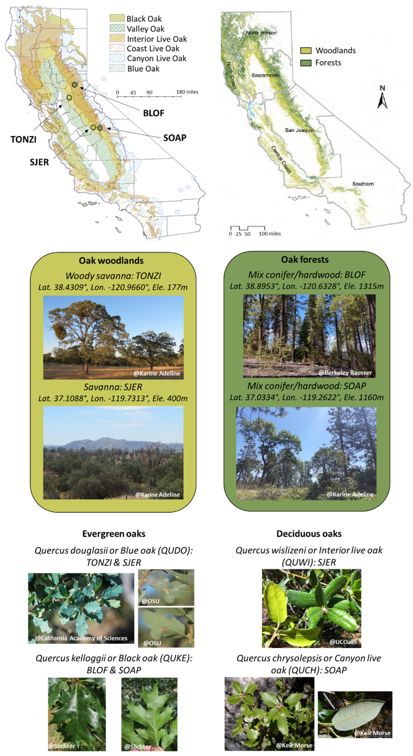
Figure 1. (Top): distribution map of six endemic California oak species (adapted from [43]) and oak ecosystem types, woodlands (including savannas) and forests (adapted from [4]). (Middle): descriptive photos of the four study sites with their geographic coordinates. (Bottom): photos of the leaves (adaxial and abaxial side) of the four studied oaks with their scientific name, common name, acronym in brackets (following the USDA Plant Database, https://plants.usda.gov/), and sites where they were sampled.
Remotesensing 16 00029 g001
Figure 2. Boxplot of leaf trait values pooled by tree species. Whiskers indicate minimal and maximal values.
Remotesensing 16 00029 g002
Figure 3. Organization chart of methods. For detailed description of the used acronyms, please refer to the following subsections.
Remotesensing 16 00029 g003
Figure 4. Influence of the leaf structural parameter N on PROSPECT simulations for the following leaf composition: Cab = 33 µg·cm−2, Cxc = 8.7 µg·cm−2, EWT = 0.015 cm, and LMA = 0.015 g·cm−2.
Remotesensing 16 00029 g004
Figure 5. Histograms of estimated PROSPECT leaf structural parameter N values for each species and per plant functional type (light and dark green: evergreen, orange and red: deciduous).
Remotesensing 16 00029 g005
Figure 6. Boxplot representation of PROSPECT leaf structural parameter N distribution for all species. Whiskers depict minimal and maximal values.
Remotesensing 16 00029 g006
Figure 7. Comparison between measured LMA and estimated values of PROSPECT leaf structural parameter N.
Remotesensing 16 00029 g007
Figure 8. Validation plots for Cab for the methods highlighted in Table 7: per species (top) and per season (bottom).
Remotesensing 16 00029 g008
Figure 9. Validation plots for Cxc for the methods highlighted in Table 9: per species (top) and per season (bottom).
Remotesensing 16 00029 g009
Figure 10. Validation plots for EWT for the methods highlighted in Table 11: per species (top) and per season (bottom).
Remotesensing 16 00029 g010
Figure 11. Validation plots for LMA for the methods highlighted in Table 13: per species (top) and per season (bottom).
Remotesensing 16 00029 g011
Figure 12. Validation plots for EWT for IO-PROSPECT, STAT-ANGERS-Ridge, and STAT-CSTARS-GPR. Color indicates the value of PROSPECT structural parameter N estimated through PROSPECT-IO. Spring leaves of QUKE(d) with a value of N below 1.2 are clearly identifiable in the IO-PROSPECT method plot.
Remotesensing 16 00029 g012
Table 1. Dates of field campaigns (format DD/MM).
Site20132014
SummerFallSpringSummerFall
BLOF-30/0922/0402/0604/11
SJER19/0607/1111/0411/0621/10
SOAP16/0609/1112/0414/0628/10
TONZ11/0624/0917/0406/0606/10
Table 2. Sample distribution for each species, season, and site.
BLOFSJERSOAPTONZTotal
SpeciesSeason
QUKE(d)Spring6-5-11
Summer4-9-13
Fall--7-7
Total10-21-31
QUCH(e)Spring--5-5
Summer--2-2
Fall--12-12
Total--19-19
QUDO(d)Spring-5-510
Summer-9-817
Fall-8-917
Total-22-2244
QUWI(e)Spring-3--3
Summer-8--8
Fall-9--9
Total-20--20
TOTAL114
Table 3. Basic statistics of CSTARS dataset (ours) compared to ANGERS dataset for the four leaf traits.
ANGERS/CSTARSCab (µg·cm−2)Cxc (µg·cm−2)EWT (cm)LMA (g·cm−2)
Mean33.6/33.98.7/8.70.0112/0.01160.0124/0.0052
Standard Dev.13.2/21.72.8/5.10.0026/0.00490.0043/0.0036
Min.0.8/0.50.0/2.00.0044/0.00500.0017/0.0045
Max.106.7/68.425.3/17.80.0340/0.02020.0331/0.0215
Table 4. Correlation matrix for the four leaf traits obtained by pooling all species, sites, and seasons.
CabCxcEWTLMA
Cab1.000.920.240.52
Cxc 1.000.260.66
EWT 1.000.43
LMA 1.00
Table 5. Optimal q * values of LUT-based strategies for each sampling scheme and distance function.
CabCxcEWTLMA
LUT-GV-MSE20075031000
LUT-GV-SAM5001500350
LUT-LH-MSE8322000
LUT-LH-SAM15020002200
Table 6. Basic statistics of estimated PROSPECT leaf structural parameter N by species and sites.
SpeciesQUCH(e)QUWI(e)QUKE(d)QUDO(d)
SiteSOAP
(n = 19)
SJER
(n = 20)
BLOF
(n = 10)
SOAP
(n = 21)
All
(n= 31)
SJER
(n = 22)
TONZ
(n = 22)
All
(n = 44)
Mean2.131.811.271.481.421.791.681.74
Std.0.140.230.170.150.180.110.110.12
Med.2.121.851.211.581.461.781.691.73
Min.1.851.371.041.191.041.621.461.46
Max.2.362.181.541.771.772.051.932.06
Table 7. Performance of methods for the estimation of Cab (in each subcategory, the most accurate method is highlighted in bold).
CategoryMethodRMSE (µg/cm2)R2Bias
(µg/cm2)
PhysicalIO-PROSPECT7.80.644.9
LUT-GV-MSE8.00.634.9
LUT-GV-SAM8.00.635.5
LUT-LH-MSE13.5−0.0511.5
LUT-LH-SAM14.3−0.1912.4
HybridHybrid-Ridge11.30.269.2
Hybrid-PLSR11.80.199.5
Hybrid-GPR9.00.535.8
Hybrid-RFR8.60.575.8
StatisticalSTAT-ANGERS-Ridge12.90.0411.7
STAT-ANGERS-PLSR10.30.398.7
STAT-ANGERS-GPR9.40.496.3
STAT-ANGERS-RFR11.50.247.0
STAT-CSTARS-Ridge6.40.710.3
STAT-CSTARS-PLSR5.80.760.2
STAT-CSTARS-GPR5.00.83b
STAT-CSTARS-RFR5.70.780.1
Table 8. Detailed results of STAT-CSTARS-GPR/IO-PROSPECT for Cab.
RMSE
(µg/cm2)
R2Bias
(µg/cm2)
SpeciesQUCH(e)6.4/4.30.71/0.881.0/0.6
QUWI(e)4.6/4.50.80/0.870.9/1.8
QUDO(d)4.6/9.90.76/−0.201.1/8.1
QUKE(d)3.0/9.40.73/0.360.3/7.1
SeasonSpring3.7/7.00.93/0.78−1.2/3.4
Summer5.8/9.2−0.02/−0.151.2/6.2
Fall4.8/7.00.81/0.732.1/4.7
Table 9. Performance of methods for the estimation of Cxc (in each subcategory, the most accurate method is highlighted in bold).
CategoryMethodRMSE (µg/cm2)R2Bias
(µg/cm2)
PhysicalIO-PROSPECT2.00.50.4
LUT-GV-MSE2.10.460.3
LUT-GV-SAM2.70.080.7
LUT-LH-MSE4.7−1.754.3
LUT-LH-SAM3.6−0.562.4
HybridHybrid-Ridge2.30.360.5
Hybrid-PLSR2.30.370.0
Hybrid-GPR2.00.520.1
Hybrid-RFR2.00.520.6
StatisticalSTAT-ANGERS-Ridge5.0−2.134.6
STAT-ANGERS-PLSR5.6−2.835.1
STAT-ANGERS-GPR3.0−0.092.0
STAT-ANGERS-RFR2.80.061.5
STAT-CSTARS-Ridge1.40.700.1
STAT-CSTARS-PLSR1.40.690.1
STAT-CSTARS-GPR1.30.750.1
STAT-CSTARS-RFR1.40.700.1
Table 10. Detailed results of STAT-CSTARS-GPR/HYBRID-GPR/IO-PROSPECT for Cxc.
RMSE
(µg/cm2)
R2Bias
(µg/cm2)
SpeciesQUCH(e)1.9/2.6/2.30.47/0.19/0.370.8/−0.8/0.3
QUWI(e)1.3/2.5/2.20.69/0.17/0.320.2/−1.4/−1.5
QUDO(d)1.0/1.4/1.90.63/0.23/−0.460.4/0.1/0.5
QUKE(d)0.7/1.8/1.80.75/0.12/0.160.0/1.6/1.5
SeasonSpring1.1/2.2/2.20.90/0.60/0.620.1/−0.1/0.9
Summer1.5/1.7/2.00.21/0.18/−0.170.6/0.3/0.9
Fall1.2/2.0/1.90.72/0.57/0.620.5/0.0/−0.4
Table 11. Performance of methods for the estimation of EWT (in each subcategory, the most accurate method is highlighted in bold).
CategoryMethodRMSE
(cm)
R2Bias
(cm)
PhysicalIO-PROSPECT0.00350.730.0018
LUT-GV-MSE0.0037−0.900.0020
LUT-GV-SAM0.0034−0.630.0019
LUT-LH-MSE0.0034−0.660.0017
LUT-LH-SAM0.00330.500.0018
HybridHybrid-Ridge0.0070−5.930.0063
Hybrid-PLSR0.0069−5.660.0061
Hybrid-GPR0.0052−2.840.0030
Hybrid-RFR0.00431.560.0029
StatisticalSTAT-ANGERS-Ridge0.00160.660.0001
STAT-ANGERS-PLSR0.00180.52−0.0007
STAT-ANGERS-GPR0.00180.530.0004
STAT-ANGERS-RFR0.0048−2.290.0036
STAT-CSTARS-Ridge0.00090.870.0001
STAT-CSTARS-PLSR0.00100.830.0000
STAT-CSTARS-GPR0.00090.870.0001
STAT-CSTARS-RFR0.00150.620.0000
Table 12. Detailed results of STAT-CSTARS-GPR/STAT-ANGERS-Ridge for EWT.
RMSE
(cm)
R2Bias
(cm)
SpeciesQUCH(e)0.0015/0.00140.76/0.71−0.0002/0.0004
QUWI(e)0.0010/0.00120.31/0.350.0003/0.0004
QUDO(d)0.0009/0.00120.58/0.330.0006/0.0006
QUKE(d)0.0012/0.00220.83/0.52−0.0003/−0.0018
SeasonSpring0.0013/0.00170.67/0.220.0002/−0.0006
Summer0.0010/0.00170.88/0.570.0002/−0.0001
Fall0.0010/0.00130.86/0.780.0003/0.0001
Table 13. Performance of methods for the estimation of LMA (in each subcategory, the most accurate method is highlighted in bold).
CategoryMethodRMSE (g/cm2)R2Bias
(g/cm2)
PhysicalIO-PROSPECT0.0055−0.640.0038
LUT-GV-MSE0.00380.200.0017
LUT-GV-SAM0.00210.760.0014
LUT-LH-MSE0.0049−0.290.0037
LUT-LH-SAM0.00300.520.0026
HybridHybrid-Ridge0.0071−1.720.0071
Hybrid-PLSR0.0069−1.610.0041
Hybrid-GPR0.0062−1.120.0038
Hybrid-RFR0.00300.50.0014
StatisticalSTAT-ANGERS-Ridge0.00130.91−0.0006
STAT-ANGERS-PLSR0.00130.91−0.0003
STAT-ANGERS-GPR0.00160.860.0005
STAT-ANGERS-RFR0.0044−0.04−0.0024
STAT-CSTARS-Ridge0.00090.950.0000
STAT-CSTARS-PLSR0.00090.950.0000
STAT-CSTARS-GPR0.00090.950.0000
STAT-CSTARS-RFR0.00130.900.0000
Table 14. Detailed results of STAT-CSTARS-GPR/STAT-ANGERS-Ridge for LMA.
RMSE
(g/cm2)
R2Bias
(g/cm2)
SpeciesQUCH(e)0.0011/0.00170.60/0.20−0.0001/−0.0012
QUWI(e)0.0012/0.00230.64/−0.04−0.0003/−0.0020
QUDO(d)0.0008/0.00070.79/0.810.0002/−0.0001
QUKE(d)0.0007/0.00070.82/0.80−0.0000/−0.0002
SeasonSpring0.0008/0.00130.98/0.940.0001/−0.0005
Summer0.0009/0.00140.92/0.830.0001/−0.0006
Fall0.0011/0.00130.91/0.89−0.0001/−0.0007
Disclaimer/Publisher’s Note: The statements, opinions and data contained in all publications are solely those of the individual author(s) and contributor(s) and not of MDPI and/or the editor(s). MDPI and/or the editor(s) disclaim responsibility for any injury to people or property resulting from any ideas, methods, instructions or products referred to in the content.