Abstract
Owing to the dependence of algorithms on the measurement of ship soundings and geophysical parameters, the accuracy and coverage of topography still need to be improved. Previous studies have mostly predicted topography using gravity or gravity gradient, However, there is a relative lack of integrated research combining or comparing gravity and gravity gradient. In this study, we develop observation equations to predict topography based on vertical gravity anomalies (VG; also called gravity anomalies) and vertical gravity gradient (VGG) anomalies generated by a rectangular prism. The sources of interference are divided into medium- to high-frequency errors and low-frequency errors, and these new methods reduce these errors through regularization and error equations. We also use numerical simulations to test the efficiency of the algorithm and error-reduction method. Statistics show that VGG anomalies are more sensitive to topographic fluctuations; however, the linear correlation between VG anomalies and topography is stronger. Additionally, we use the EIGEN-6C4 model of VG and VGG anomalies to predict topography in shallow and deep-sea areas, with maximum depths of 2 km and 5 km, respectively. In the shallow and deep-sea areas, the root mean square (RMS) errors of VGG anomalies prediction are 93.8 m and 233.8 m, and the corresponding accuracies improved by 7.3% and 2.3% compared with those of VG anomaly prediction, respectively. Furthermore, we use cubic spline interpolation to fuse ship soundings and improve the accuracy of the final topography results. We develop a novel analytical algorithm by constructing an observation equation system applicable to VG and VGG anomalies. This will provide new insights and directions to refine topography prediction based on VG and VGG anomalies.
1. Introduction
Since the release of the first version of the global elevation product ETOPO-5 by the National Oceanic and Atmospheric Administration (NOAA) in 1998, major institutions worldwide have been refining and releasing global topography models. For example, the Technical University of Denmark (DTU) has released a global topography model with a resolution of 1 arcmin in 2010 [1]. Recently, the International Hydrographic Organization (IHO) released global topography GEBCO-2021 with a resolution of 15 arcseconds by combining high-precision gravity and abundant ship soundings data. However, the topography is obtained by interpolation in most sea areas with low accuracy [2]. Although direct measurement has the advantages of high resolution and accuracy, the time and financial costs are impractical [3]. Some deep seas and sea areas cannot be covered by ship surveys, because of the harsh environmental conditions. Therefore, using satellite data is an effective approach to the prediction of topography.
Currently, methods of topography prediction have mostly employed vertical gravity (VG) anomalies data, and the algorithms are primarily based on the gravity–geologic method (GGM) and frequency method based on Parker’s formula [4,5,6,7,8,9,10]. The GGM separates short-wave signals from the VG anomalies, fits the optimal functional relationship between the ship soundings data and VG anomalies, and adjusts the density constant to achieve the best fitting effect [11,12]. However, VG anomalies are mainly obtained from altimetry satellites [13,14,15], and relatively large errors occur in the nearshore and island reefs. To rectify this problem, the ICESat series of lidar satellites and the Sentinel series of optical imaging satellites are mainly used to predict shallow water depths, especially those at nearshore regions and island reefs [16,17,18]. Moreover, for water depths below 40 m, the root mean square (RMS) error of the prediction results was generally less than 1 m [19,20]. Additionally, Hsiao et al. used the GGM combined with satellite image data to improve the accuracy of topography prediction near 41 islands and reefs by 50% to 97% in the South China Sea [5]. Similarly, Rasheed et al. combined image satellites and topography models to refine the topography of the Maldives, in what was a robust attempt at multi-source data fusion [21]. Moreover, by relying on Parker’s potential Fourier expansion formula, the relationship between VG anomalies and seabed depth was established in the frequency domain [22]. This method considers the selection of various geophysical parameters and wavebands of the gravitational field in the study sea area. Dixon et al. have suggested that topography and geoid height are highly correlated in the wavelength range of 50–300 km [23]. Combined with results of previous studies, Smith and Sandwell used more accurate VG anomaly data to show that topography and VG anomalies may exhibit a linear correlation in the range of wavelengths between 15–160 km [24].
A number of studies have used vertical gravity gradient (VGG) anomalies to predict topography, as VGG anomalies are more sensitive to topographic fluctuations than VG anomalies. The least-squares method was used to predict topography using VGG anomalies by Wang [25]; however, it was limited only to the derivation of theoretical formulas. Nagy et al. derived an analytical expression for the gravitational field generated by a rectangular prism and highlighted its potential applications in Earth sciences [26]. Based on Nagy’s research, Yang et al. used a simulated annealing method, combined with VGG anomalies, to form an algorithm for the statistical analysis of VGG anomalies data, which in turn was used to predict topography [27]. Yu et al. used the VGG anomalies formula generated by a rectangular prism to establish an observation equation between VGG anomalies and sea depth to predict topography [28].
Although a variety of global topography models have been developed using gravity anomalies [29,30,31,32], insufficient ship soundings data, resolution and error of gravity field models, etc., restrict the accuracy of current global topography models [33]. Therefore, the Surface Water and Ocean Topography (SWOT) satellite altimetry plan aims to improve the resolution and accuracy of marine gravity anomalies to 1 km and 1 mGal, respectively, and the corresponding accuracy of topography can reach 70 m [34,35]. Additionally, Seabed 2030, a joint project between the Nippon Foundation and the General Bathymetric Chart of the Oceans (GEBCO), aims to improve the resolution of their topography model from below 3000 m to within 200 m by enhancing ship soundings data [36]. In summary, VG anomalies and ship soundings data are the primary sources for current topographic prediction. A new method for predicting topography, combined with other gravity field data, especially VGG anomalies, should be further studied to refine the global topography model.
Accordingly, we used the analytical formulas of VG and VGG anomalies generated by a rectangular prism to establish the observation equation between sea depth and VG and VGG anomalies to predict topography in Section 2.1. Due to the existence of errors, we further refine the sources of the interference errors, quantitatively analyze their magnitude through numerical simulations and investigate methods to reduce corresponding errors in Section 2.2. In Section 2.3, we use a cubic spline algorithm to fuse ship-sounding. Subsequently we apply the algorithm to actual predictions in Section 3. Furthermore, we use cubic spline interpolation to fuse ship soundings and prediction topography to obtain the final topography results. Our algorithm does not heavily rely on ship soundings data and is able to predict topography with any resolution of VG and VGG anomaly models, providing new ideas and methods for the improvement of global topography models in the future.
2. Method and Theory
In this section, based on VG and VGG anomalies generated by a single prism, we establish the theory and method of predicting topography. Then, the source of interference error is refined and the corresponding algorithm proposed, and the cubic spline algorithm is used to fuse ship-sounding.
2.1. Establishment of Observation Equations
The topography can be approximately discretized into multiple rectangular prisms as shown Figure 1, so we obtain the height of each prism to predict topography. The local coordinate system is shown in Scheme A1 (Appendix A.1), where the length, width and height of the rectangular Ω are 2a, 2b and H − h respectively, thus the gravitational potential generated by Ω at point P can be expressed as
where G is the gravitational constant (), is the density of Ω, and is the integral variable. Based on previous work [26,37,38], the VG and VGG generated by Ω at point P can be expressed as
where .
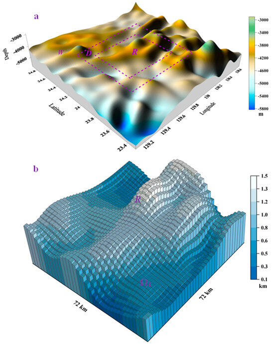
Figure 1.
(a) Simulated topography from ETOPO-1 and (b) schematic diagram of the study area R after 2 km gridding.
Thus, the expression of VG and VGG generated by Ω at any point P is obtained.
The above discussion is based on a single prism. Determining the sea depth of each prism can help obtain the topography. Therefore, we assume that is a square area on the sea surface (such as Figure 1b), and is the corresponding topography, where is the height from the top of Ω1 to the sea surface. Because the methods of constructing observation equations using VG and VGG anomalies are similar, this section will mainly derive from VG anomalies generated by Ω1.
The step length is set as t, and the interval is divided into 2N equal parts. Thus, the area R can be gridded, and the typical sub-grid areas are , , . If the t is small enough, in the sub-grid area Rij can be regarded as a constant . From Appendix A.2, using Equations (A1) and (A2) and the principle of superposition, the VG generated by Ω1 at sea level can be expressed as
Removing the influence of sea water from Equation (4), the VG anomalies generated at P in the sea area R can be rewritten as
where , and are the densities of bedrock and seawater, respectively. If the observed value of VG anomalies in the sea area R can be obtained in advance, we have
where is the observation point in sea surface R, and .
Thus, Equation (6) of topography is established from VG anomalies, and is the average depth of sub-grid . In Equation (6), the number of equations is and that of unknowns is , thus, the solvable condition is theoretically satisfied. As Equation (6) is nonlinear with respect to , it can be solved by the Newton iterative method after obtaining the initial value . Combined with Equation (A4) in Appendix A.2, the kth iteration equation is expressed as follows:
Using the same construction method in combination with Appendix A.3, the observation equations for VGG anomalies are as follows:
Equations (7) and (8) are final iterative equations for solving topography from VG and VGG anomalies. Consequently, when the VG and VGG anomalies are provided in advance, we can predict topography by solving Equations (7) or (8). The above discussion refers to the case of no error interference. Nevertheless, the impact of errors cannot be ignored. Therefore, we will study the source of errors and reduce the sources of them in the next section.
2.2. Identification and Reduction Interference Errors
Section 2.1 focuses only on the rectangular prism or the study sea area; however, the actual topography is more complicated. In this section, the error sources are mainly divided into boundary and far areas, and the magnitude of effects is estimated through simulations. We consider the topography model shown in Figure 1a as an example (the topography model is from ETOPO-1 and is also chosen as the case study for comparison in Section 3), wherein R is the study area. Nevertheless, the topographic fluctuation outside R impacts on the observation data of VGG anomalies at R. The influence of topographic fluctuations 10 km away from R on the observed VGG anomalies at R is a low-frequency characteristic [28]. Therefore, we divided the area outside R into boundary areas D and far area W (shown in Figure 1a). The boundary area D is 10 km adjacent to R, and the distance beyond 10 km is called the far area W.
Figure 1a shows the simulated topography of an area of 160 km × 160 km, where R has an area of 72 km × 72 km, the adjacent 10 km represents D, and the area outside D is W. The 2 km ×2 km grid of R is shown in Figure 1b. Using forward computations in Equations (2) and (3), the VG and VGG anomalies generated by R above the sea level are shown in Figure 2a,b. Figure 2b shows that the VGG anomalies are more similar to the topography than the VG anomalies; in other words, the VGG anomalies are more sensitive to deep mass change, and previous studies have also confirmed this conclusion [39,40].
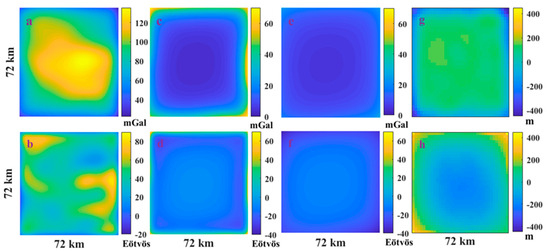
Figure 2.
(a,b) VG and VGG anomalies generated from the study area R, (c,d) VG and VGG anomalies generated by the boundary area D in the study area R, (e,f) VG and VGG anomalies generated by the far area W in the study area R, (g,h) error distribution for simulated prediction results using VG and VGG anomalies.
The VG and VGG anomalies obtained by forward computations are used to solve the VG and VGG observation equations—Equations (7) and (8), respectively. The RMS error of the prediction results is reduced to 10−5 m, and the RMS error curve corresponding to the number of iterations is shown in Figure 3a. Figure 3a shows that Equations (7) and (8) are convergent. However, the convergence rate of Equation (8) is significantly better than that of Equation (7). That is, the convergence of the observation equation established by the VGG anomalies is better.
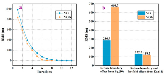
Figure 3.
(a) Diagram of the iteration number and RMS error for the VG and VGG observation equation. (b) RMS errors of prediction results using different processing methods for VG and VGG anomalies.
In the above section, we verify the observation equations in Equations (7) and (8) without errors; simultaneously, the influence of D and W on the VG and VGG anomalies above R cannot be ignored. The VG anomalies generated by D on R are shown in Figure 2c, and its range is 67.9 mGal, as shown in Table 1 (the maximum and minimum values are 71.3 mGal and 3.4 mGal at the boundary and center, respectively, as shown in Figure 2c), indicating that the VG anomalies generated by D on R show obvious boundary effects. The VG anomalies generated by W on R is relatively flat (shown in Figure 2e); this is evident from the decrease in standard deviation (SD) from 14.5 mGal to 4.1 mGal (presented in Table 1).

Table 1.
Statistical results of VG and VGG anomalies generated in study area R.
We directly use VG and VGG anomalies in R as the observation values (including three parts: the study area R, boundary area D and far area W). Subsequently, D and W can be regarded as interference errors, which result in the lack of convergence of the solutions of Equations (7) and (8). Through numerous simulations, we finally use the regularization algorithm and introduce an error equation to deal with D and W, respectively.
The regularization algorithm of this study is as follows: we use only the simulated VGG anomaly data of R to solve the topography of R and D, and then the topography of D is then removed, and only that of R is reserved as the final prediction result.
Thus, Equation (6) can be rewritten as
where M is the number of grids at D, as the distance of D is selected as 10 km relative to the five grids, that is, . Subsequently, Equation (9) has a total of (4N + 1)2 equations. Similar to Equation (7), Equation (9) can be linearized, and the linearized equations can be simplified to Ah = b, where A is the matrix of (4N + 1)2 × (2N + 5)2, h is the (2N + 5)2 order vector of the unknown depth to be solved, and b is the VGG anomalies observation matrix of the (4N + 1)2 order vector. As all of the observation points are in R, the linearized equation Ah = b may produce a singularity. To ensure the solvability of Equation (9), the regularization equations are introduced as follows
where E is the identity matrix of the (2N + 5)2 × (2N + 5)2 order, and is the regularization parameter.
As , there is always a unique solution for Equation (10) with respect to h.
Therefore, after iteratively solving Equation (10), can be solved.
Figure 2e,f show that the VG and VGG anomalies generated by W in R exhibits low-frequency characteristics. Therefore, the low-frequency error generated by W is regarded as a constant, and is introduced into Equation (10), and the observation equations are then rewritten with error terms as follows:
Equation (11) is the observation equation to deal with D and W.
Through Equations (10) and (11), the statistical RMS error of the simulated prediction results are shown in Figure 3b. Using only the regularization algorithm to process the influence of D, the RMS errors of the VG and VGG anomalies are estimated as 286.9 m and 660.7 m, respectively. Compared with the non-convergence results obtained by directly solving Equations (7) and (8), the regularization algorithm can significantly improve the accuracy; however, the simulated prediction results of VG anomalies are more effective and their resistance to low-frequency errors is better (because the solution obtained using only regularization does not consider the influence of far area W). When solving Equation (11), the RMS errors corresponding to VG and VGG anomalies are 132.5 m and 118.2 m respectively, which improves the accuracy by 53.8% and 82.1%, respectively, and indicates that the simulated prediction results using VGG anomalies will be better. Compared with that of the simulated results of Equations (10) and (11), the interference of W has a greater impact on the simulated prediction results when using VGG anomalies. This is mainly ascribed to the lower signal-to-noise ratio of the VGG anomalies: from the mean value presented in Table 1, the VG and VGG anomalies generated by W account for 10.8% (9.9 mGal/91.4 mGal) and 41.5% (16.9 Eötvös/40.7 Eötvös) of that generated by the R itself. Additionally, the simulated error distributions when dealing with D and W are shown in Figure 2g,h. The larger errors are mainly distributed at the boundary, and the error gradually decreases toward the center. For an obvious boundary effect, a larger area is usually solved, and the boundary is intercepted to improve the accuracy of the results.
2.3. Cubic Spline Interpolation Algorithm for Fusing Ship Soundings
Although topography can be predicted independently by solving the equation—Equation (11)—established using gravity data, its accuracy is lower than the ship soundings. In this section, we will combine the cubic spline interpolation algorithm to fuse the prediction results and ship soundings. Notably, the use of gravity data to predict topography is not only to completely replace ship soundings, but to also fill in the blank areas left by ship soundings to improve the accuracy and resolution of topography model.
The expression of the cubic spline basis function is:
The split point is , where , and h is the step size. The interpolation condition function is:
At this time, the expression of cubic spline interpolation is:
Combining Equations (13) and (14), we have:
Rewriting Equation (15) in matrix form, we obtain:
where matrix B is the two-dimensional array corresponding to array c that is arranged out.
For ship soundings, the interpolation condition function is as follows:
Similarly, the following equations can be obtained:
Equation (18) in matrix form is as follows:
where c is still the vector to be solved formed by the interpolation coefficients of Equation (14), and the matrix B1 is formed using in Equation (18).
Combining Equations (16) and (19), we have:
where the vector c must be solved. Finally, the least-square method is used to solve Equation (20), which involves determining the coefficients of Equation (14) such that Equation (14) can be obtained. This enabled us to generate various images of the fused surfaces.
In Equation (20), the matrices B and B1 are equally weighted. However, in actual calculations, Equations (18) or (19) are obtained from ship soundings, and the corresponding weight coefficients can be attributed, then Equation (20) can be rewritten as
Equation (21) is the cubic spline interpolation fusion equation using gravity data to predict topography results and ship soundings. In Section 3.4, we use Equation (21) to fuse ship soundings with different proportions and different weights w.
3. Application to Different Sea Depths
We select two sea areas to compare the difference between VG and VGG when predicting topography, to evaluate the prediction results, and to fuse ship soundings by cubic spline interpolation algorithm.
3.1. VG and VGG Anomalies Data
The previous sections have demonstrated the effectiveness of our algorithm in predicting topography from the VG and VGG anomalies through numerical simulations. In this section, we select two sea areas with different depths to compare and study the VG and VGG anomalies algorithm. The selected VG and VGG anomaly models for Sea Area-1 and Sea Area-2 are EIGEN-6C4 from the German Research Center for Geosciences (GFZ, http://icgem.gfz-potsdam.de/tom_longtime), corresponding to the grid with a resolution of 2 km × 2 km, and are shown in Figure 4(a1,a2,b1,b2). The VG and VGG anomaly model data for the two sea areas are counted as shown in Table 2. The standard deviation (SD) of the VG and VGG anomalies model data for Sea Area-1 is slightly smaller than that for Sea Area-2. We infer that the topography of Sea Area-2 is a more undulating topography, which can also be verified by the final prediction results.
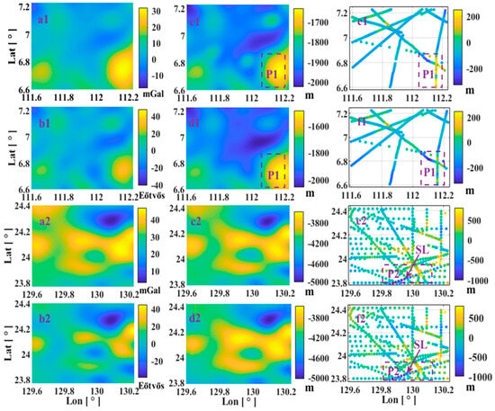
Figure 4.
(a1,b1) VG and VGG anomalies models of Sea Area-1, (c1,d1) the prediction results of the VG and VGG anomalies in Sea Area-1, (e1,f1) the prediction error distribution of the VG and VGG anomalies in Sea Area-1 (compared with the existing ship survey depth). (a2,b2) VG and VGG anomalies models from Sea Area-2, (c2,d2) the prediction results of the VG and VGG anomalies in Sea Area-2, (e2,f2) the prediction error distribution of the VG and VGG anomalies in Sea Area-2 (compared with the existing ship survey depth).

Table 2.
Statistics of the data of VG and VGG anomalies model and final prediction results.
3.2. Ship Soundings Data
The ship soundings data are obtained from NOAA’s National Geophysical Data Center (NGDC, http://www.ngdc.noaa.gov/), and their distribution is shown in Figure 4(e1,e2). There are 381 ship survey points in the selected Sea Area-1, and the deepest, shallowest, and average sea depth are −2050.0 m, −1430.0 m and −1953.4 m, respectively. There are 501 ship survey points in Sea Area-2, and their maximum, minimum and average depths are −5249.0 m, −3280.0 m and −4094.3 m, respectively. As we use grids with resolutions of 2 km, we also grid the ship soundings data of the two sea areas with a resolution of 2 km, and obtain 216 and 398 grids of ship soundings, respectively. The number of grid depths to be solved is 1296 and the existing gridded ship soundings data in Sea Area-1 and Sea Area-2 account for 16.7% (216/1296) and 30.7% (398/1296), respectively. The main objective of topography prediction is to better determine the depth of the sea area without ship soundings data.
3.3. Evaluation of the Results
Based on the VG and VGG anomalies model of EIGEN-6C4, combined with Equation (11) in the simulation experiments, the prediction results for Sea Area-1 and Sea Area-2 are shown in Figure 4(c1,d1) and Figure 4(c2,d2), respectively. Among these, Figure 4(c1,d1) correspond to the topography predicted by VG and VGG anomalies model for Sea Area-1, and the maximum, minimum and mean depths of the corresponding prediction results are given in Table 2. It can be seen that the biggest difference in depth between the VG and VGG predictions is only 147.0 m (−1632.1 m and −1485.1 m) indicating the minimum depth between the VG and VGG predictions. This mainly occurs in Area-P1, as shown in Figure 4(c1,d1). The statistical prediction results suggest that the maximum and minimum errors of VG and VGG anomaly prediction results are also concentrated in Area-P1 of Figure 4(e1,f1). This is because topographic fluctuation is large and adjacent to the boundary area, resulting in large errors. In particular, we use a 2 km × 2 km grid, where the horizontal resolution of the final prediction result is 2 km. Here, the mean depth will be less representative with increasing the topographic fluctuation. However, the accuracy of the VG and VGG anomaly model is restricted and the signal-to-noise ratio is worse with greater topographic fluctuations. However, the RMS errors are 101.2 m and 93.8 m, respectively, indicating that the relative accuracy of topography prediction using VGG anomalies is improved by 7.3% compared with that using VG anomalies.
For Sea Area-2, the difference between the prediction results of the VG and VGG anomalies is within 70 m, which is only 1.7% of the mean depth of 4100 m, indicating that the prediction results of the two are highly consistent. The prediction error statistics presented in Table 2 indicate that the RMS errors of prediction results are 239.4 m and 233.8 m, respectively, and that the relative accuracy of the VGG anomalies increased by 2.3%. The RMS error of Sea Area-2 is significantly larger than the prediction error of Sea Area-1, which is mainly attributed to depth. The accuracy of the VG and VGG anomalies model is limited, and the signal-to-noise ratio is worse with greater topographic fluctuations.
Conversely, the minimum and maximum errors of VG anomaly prediction are −1017.3 m and 760.2 m, respectively, and the larger error is concentrated on the survey line SL in the Area-P2 shown in Figure 4(e2,f2). To analyze the cause of these errors, we intercepted the depth data of the ship in Area-P2 and plot it in Figure 5a. Notably, the depth of SL is significantly greater than that of other survey lines. To investigate further, we plot the cross-section of the survey points on the survey line SL in Figure 5b (the horizontal axis represents the distance from the first measuring point). We select boxes Q1 and Q2 (shown in Figure 5a) that are adjacent to SL with other survey points, the red points indicate the survey points on SL, and the yellow points represent the survey points of the other survey lines. Despite being 251 m and 471 m from SL, the depth differences between boxes Q1 and Q2 are 729 m and 692 m, respectively (shown in Figure 5b). We converted these into slopes of 71° and 56°, respectively. However, from the predicted results (Figure 4(c2,d2)), the topographic fluctuations in Area-Q1 and Area-Q2 are not as significant as indicated by the slopes.
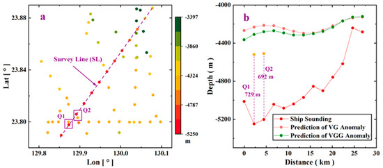
Figure 5.
(a) Distribution map of ship soundings data in Area-P2; (b) ship soundings data along the survey line SL and the prediction result of VG and VGG anomalies.
Additionally, we also plot the depth of VG and VGG anomaly prediction results along SL as the pink and green dotted lines in Figure 5b. The depth of the two prediction results is in good agreement, and the depth of the ship survey along SL is significantly greater than that of the prediction results. However, the predicted depth is closer to those of the other two survey points for Area-Q1 and Area-Q2. Furthermore, we assume that the ship soundings accuracy of SL is higher, which in turn suggests the presence of valleys with fluctuations close to 1 km along this survey line. These large topographic fluctuations can easily be recognized from the VG and VGG anomalies but are not observed in the VG and VGG anomalies model of EIGEN-6C4. Therefore, we suspect a large error in the ship survey depth along SL. It is worth noting that the ship soundings data used in this study are single-beam data from decades ago, and its measurement accuracy may have possessed errors [41]. With the development of multi-beam measurements, this problem can be improved to a certain extent; however, we are unable to obtain the multi-beam data of the predicted sea area in this study.
3.4. Fusion of Ship Soundings
The prediction results from Section 3.3 indicate that the topographic results predicted from VGG anomalies are slightly better than those of VG anomalies. Therefore, based on the results of VGG anomalies prediction in Figure 4(d1,d2), we use the cubic spline interpolation algorithm discussed in Section 2.3 to fuse ship soundings. We vary the proportions of ship soundings, set different weight coefficients w, and the final statistical error results are shown in Appendix A.4.1. Specifically, η1 represents the ratio of ship soundings used for fusion to the grid depth to be solved, η2 is the ratio of ship depth data used for interpolation to the total ship survey data, η3 indicates the improved accuracy of topography results after fusion, and w denotes the selected weight coefficient.
The statistics presented in Appendix A.4.1 demonstrate that increasing the proportion of fused ship soundings η2 and the weight coefficient w results in smaller RMS error for the fused topography results. Moreover, we separately evaluated the RMS error for the ship soundings used in the fusion (RMSFusing) and the remaining ship soundings used as checking (RMSChecking). The results in Appendix A.4.1 reveal that the RMS error of ship soundings involved in the fusion is significantly smaller than that of the remaining ship soundings points. The improvement in the accuracy of the final topographic result is represented by η3. As the weight coefficient w increases, the accuracy of Sea Area-1 increases from 0.06% to 53.20%, whereas that of Sea Area-2 increases from 2.9% to 32.63%.
Furthermore, by setting η2 to 50% and w to 0.6, we draw topography results, shown in Figure 6. Notably, Figure 6a shows that the final fused topography result of Sea Area-1 exhibits obvious ship track banding phenomenon, whereas that of Sea Area-2 appears smoother. This can be attributed to the fact that the maximum fluctuation of Sea Area-1 is only 400 m, resulting in more obvious errors, the maximum fluctuation of Sea Area-2 is around 1500 m, which tends to reduce the fluctuation caused by errors. Additionally, the gravity data model produces smoother results, which results in correspondingly smoother predicted topography results. However, the actual topography is not completely smooth, making it difficult to seamlessly integrate the prediction topography results with ship soundings and resulting in error distribution along the ship survey lines.
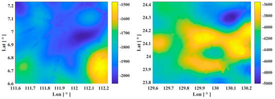
Figure 6.
(left) The topography distribution result of Sea Area-1 when 50% of ship soundings are fused and the weight is set to 0.6. (right) The topography distribution result of Sea Area-2 when 50% of ship soundings are fused and the weight is set to 0.6.
4. Discussion
4.1. Correlation Analysis of Gravity and Topography
Specifically, Figure 7a–c show the distribution of VGG anomalies, VG anomalies and topography prediction from VGG anomalies. Comparing Area-P3 and Area-P4 of VG and VGG anomalies models, VGG anomalies change more noticeably for the same topographic fluctuations indicating that VGG anomalies are more sensitive to topography. Moreover, the range and standard deviation (SD) of the statistical VG and VGG anomalies model data (shown in Appendix A.4.2), indicate that the SD of VG and VGG anomalies in Sea Area-1 are 8.5 mGal and 10.5 Eötvös, respectively, in turn suggesting that the VGG anomaly data have greater volatility. This characteristic may enable VGG anomalies to better identify faint topographic fluctuations.
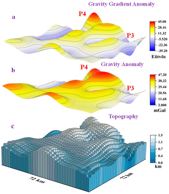
Figure 7.
(a) The VGG anomalies generated by topography, and its maximum and minimum values are 45.00 Eötvös and −39.20 Eötvös, respectively. (b) The VG anomalies generated by topography, and its maximum and minimum value are 2.80 mGal and 47.20 mGal, respectively. (c) The topographic results of VGG anomalies inversion, and its maximum and minimum heights are 1.47 km and 0.01 km, respectively.
The SD of the topographic results of Sea Area-1 predicted from VG and VGG anomalies are 122.9 m and 76.2 m, and those of Sea Area-2 are 245.1 m and 284.8 m, respectively (shown in Appendix A.4.2). This is consistent with the RMS error of the prediction results, indicating that topographic fluctuations significantly affected the accuracy of prediction results. The improved resolution of VG and VGG anomaly data may also reduce the effect of this error, thus improving the accuracy of the final prediction results. We also use numerical simulations to verify this conclusion in Appendix A.5. We simulate two symmetrical conical seamounts and use the resolutions of 4 km and 2 km for prediction respectively. The corresponding RMS errors are 56.1 m and 7.2 m, indicating that the resolution increased by 1 time and the resulting accuracy improved by 7.8 times.
Furthermore, Pearson correlation analysis was performed on the data and was used mainly to measure the strength of linear correlation between the variables. The correlation coefficient r can be calculated by the following formula:
where Xi and Yi represent each data value, and represent the average values, and n represents the data capacity. Results of the use of Equation (22) to count the correlation between topography and VG and VGG anomaly data are shown in Table 3. The correlation coefficient r between topographic results and VG/VGG anomalies ranges from 0.86 to 0.97, indicating a stronger linear correlation between the former pair of variables. The correlation coefficient r between VG anomalies and topography is greater than that of VGG anomalies, which indicates a stronger linear relationship between VG anomalies and topography. This finding supports the theoretical basis of the GGM and S&S algorithms based on Parker’s formula for predicting topography.

Table 3.
Pearson correlation between the topography and gravity models.
4.2. Comparison between Spatial and S&S Algorithm
The current topographic prediction algorithms mainly include GGM and S&S algorithms (purple box in Figure 8). These algorithms improve the accuracy by identifying the optimal band related to VG anomalies and topography. Dixon et al. initially suggested that topography and geoid height are highly correlated in the wavelength range of 50–300 km [23]. Subsequently, this band was refined to a range of 16–160 km, and a recent study has focused on improving filtering methods to enhance prediction accuracy [42]. GGM is a fitting method based on the Bouguer formula. The key to the fitting method is to determine the best fitting function and the optimal parameters. However, the Bouguer formula represents only a first-order function relationship between VG anomalies and topography. Previous studies have attempted to introduce high-order terms; however, the effect was minimal [43]. The density constant and maximum depth are most frequently adjusted variables [12]. However, the final fitted density constant often loses its original physical meaning [11]. According to prior studies, the GGM may have limitations in terms of improving the accuracy of topographic predictions. Considering that the GGM is a fitting method and given the abundance of data, machine learning and deep learning methods may be a potential direction for improvement.
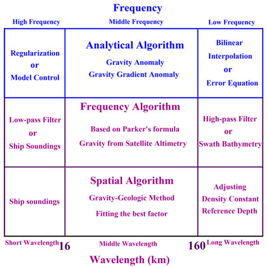
Figure 8.
Comparison of topography prediction algorithms.
Furthermore, relying on Parker’s potential Fourier expansion formula, the relationship between VG anomalies and seabed depth is established in the frequency domain [22,44,45]. However, this method needs to be combined with the deflection theory, and different geophysical parameters need to be selected for different sea areas [46,47]. As an example, the density of seabed bedrock and the thickness and density of the crust are very complex and changeable. In order to improve the accuracy of algorithm prediction, an appropriate filtering method must be chosen to remove the short-wave and long-wave interference signals from VG anomalies [48,49], while also maintaining the middle band of the topographic fluctuation corresponding to VG anomalies.
Apart from the two main methods of its predecessors, the algorithm proposed in this study is shown in the blue box in Figure 8. Based on the VG and VGG anomaly analytical formula generated via rectangular prism, we build the observation equation system for predicting topography and adopt the iterative least-squares algorithm to solve the observation equations. The interference error signals are refined from the frequency, and we mainly use the regularization algorithm, combined with the current topography model, to reduce the influence of the medium- and high-frequency error interference at the boundary of the study sea area. We used the error equation to reduce the influence of low-frequency errors caused by far sea areas and lithospheric deflection.
The line integration approach establishes the theoretical gravity formula produced by a two-dimensional geological body for the VG and VGG anomaly formula of the rectangular prisms [50]. Based on Hubbert’s work [50], Talwani et al. applied this approach to the inversion of the Mendocino submarine fault zone and discovered that the southern fault is 3 km thinner than the northern fault [51]. Subsequently, Talwani and Ewing used the numerical integration method to compute VG anomalies generated by any three-dimensional geological body and applied it to topographic correction [52]. However, this formula has been used in the inversion of density interfaces for decades [53,54,55,56] and has not been fully utilized to predict topography.
4.3. Data Precision and Prediction Algorithm
In this study, the step length of the sea area grid is 2 km, which indicates that the topographic fluctuations within 2 km × 2 km are only represented by an average sea depth, making it challenging to distinguish the topographic fluctuations within 2 km. Although the EIGEN-6C4 and EGM2008 gravity field model can reach a degree of 2160 [57], their spatial resolution is approximately 8 km. Therefore, the resolution of VG anomalies makes it challenging to reflect extreme topographic fluctuations, especially seamounts. To solve this problem, Xu et al. derived a series expression of VG and VGG anomalies generated by cylinders and superimposed the cylinders with different radii to fit the seamounts [58]. Sandwell et al. estimated the locations and shapes of seamounts using the variation characteristics of VGG anomalies generated by the different sizes of seamounts [59]. The algorithm can improve prediction accuracy but is more effective for improving the accuracy of gravity field observation data. Marine gravity anomalies were recovered from Geosat and ERS-1 with an accuracy of about 4–7 mGal [15]. With the development of altimetry satellites, the accuracy of a new marine gravity anomaly can reach about 2 mGal [39]. The next-generation surface water ocean topography (SWOT) satellites may be a revolutionary improvement in marine gravity recovery [60,61], and the SWOT ocean products will also provide 1 km spatial resolution over oceans [35]. Improvements in marine gravity anomalies are critical, while VGG anomalies and geoid height data may also have potential for topography prediction.
The algorithm proposed in this study may also provide a reference for the inversion of density models in geophysics. Similarly, the boundary effect problem of traditional geophysical inversion is generally solved by solving a larger area, but with only the inner area considered as the final result. The regularization method can also be used to address the boundary effect in this study. Additionally, the ship soundings fusion algorithm can be further improved. The use of the spatial relationship between the previous data, combined with deep learning to reduce signal noise [62,63], may be the direction of our future study. However, significant challenges remain in the prediction of topography, such as gravity signal separation and flexural isostatic problems. We performed numerous numerical tests using various filtering techniques and bilinear interpolation until we obtained the current method of reducing interference errors. Although this error reduction method may not be the best in this study, the interference error refinement is a novel idea, one that provides a potential direction for refining future topography predictions. Additionally, with an increase in data volume, our prediction algorithm is worth further research and improvement.
5. Conclusions
In summary, the main results are as follows: (1) we have developed a new analytical algorithm for predicting topography through an iterative solution from VG and VGG anomalies, and the effectiveness of this method is confirmed and verified by simulations and actual applications. (2) We have determined the source of the errors, the mid–high frequency error caused by the boundary area is reduced by regularization, whereas the low-frequency error caused by the far area is reduced by the error equation algorithm. (3) The theoretical method proposed in this study was applied to the two actual sea areas and the RMS errors of the two sea areas predicted from VGG anomalies were 93.8 m and 233.8 m, respectively, with the accuracy improved by a respective 7.3% and 2.3% compared with that of VG anomalies. Simultaneously, we use the cubic spline interpolation algorithm to effectively fuse the prediction results and ship soundings. (4) The statistical results of VG and VGG anomaly and topography prediction show that VGG anomalies are more sensitive to topography fluctuations; however, VG anomalies have a stronger linear correlation with topography, which is the basis for using gravity anomaly data to predict topography by fitting calculation.
Author Contributions
Software, computations for arithmetic examples, analysis for computational results and writing original draft, H.X. and Y.T.; derivations for main formulas, designs of computations and review paper, J.Y. and O.B.A.; analyses for actual seafloor topographies and review paper, Q.W. and Z.S. All authors have read and agreed to the published version of the manuscript.
Funding
This work is funded jointly by the National Nature Science Funds of China (Nos. 41774089, 42274010, 42204009) and the Fundamental Research Funds for the Central Universities (Nos. 2023000540, 2023000407).
Data Availability Statement
The ship soundings data are from NOAA’s National Geophysical Data Center (NGDC, https://www.ncei.noaa.gov/maps/geophysics/), one can obtain the required data by entering the latitude and longitude; VG and VGG anomaly model can be obtained from the German Research Center for Geosciences (GFZ, http://icgem.gfz-potsdam.de/tom_longtime), and the model selected in this study was “EIGEN-6C4”; the topography model can be downloaded from the German Research Center for Geosciences (GFZ, http://icgem.gfz-potsdam.de/calcgrid), one can obtain the required data by entering the latitude and longitude.
Acknowledgments
The authors wish to thank GFZ and NGDC for supplying actual data. Thanks to the anonymous reviewers for their valuable comments on this study. Thanks also go to Feng Wei of Sun Yat-sen University for his valuable suggestions in this study of writing this paper.
Conflicts of Interest
The authors declare no conflict of interest.
Appendix A
Appendix A.1. The Local Coordinate System
As shown in Scheme A1, the length, width and height of the rectangular prism Ω are 2a, 2b, H − h, respectively, where H (the maximum depth, also called the reference depth) is the height from the bottom of Ω to the sea level, and h is the height from the top of Ω to sea level. Assuming P is any point at sea level, then one must calculate the VGG generated by Ω at point P.
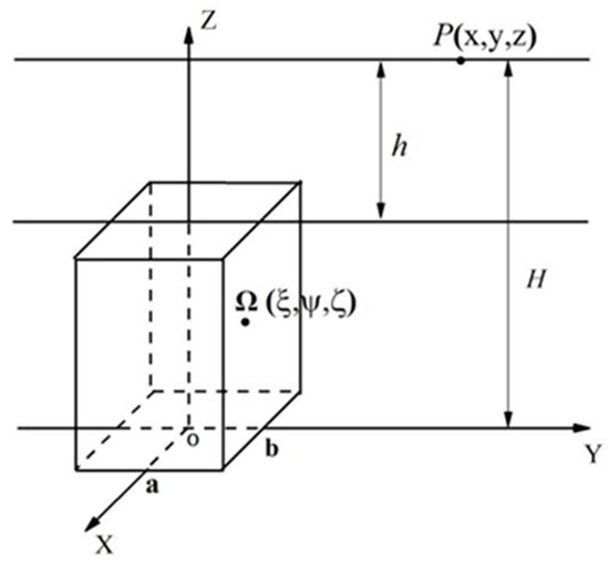
Scheme A1.
Schematic diagram of synthetic cylindrical seamount.
Appendix A.2. The Expansion Expression of VG
Equation (2) can be calculated and simplified as follows:
where can be expressed as:
where:
where and have the same expression, just replacing H with h. Meanwhile, we can calculate the expression for the derivative of with respect to h:
where is given in Equation (A6) in Appendix A.2.
Appendix A.3. Expansion Expression of VGG
Equation (3) can also be written as:
where can be expressed as:
where and have the same expression, replacing H with h. In this study, a Newton iteration is used, and the derivative of with respect to h must be calculated:
Appendix A.4. Statistical Table
Appendix A.4.1. Result Statistics of Ship Sounding Fusion
η1 represents the ratio of ship sounding used for fusion to the grid depth to be solved, η2 is the ratio of ship depth data used for interpolation to the total ship survey data, η3 is the improved accuracy of topography results after fusion, and w represents the selected weight coefficient. We separately count the RMS error of the data points involved in the fusion ship sounding, which is represented by RMSFusing. At the same time, the ship sounding points that are not used for fusion are used as checks, and the corresponding RMS error is expressed as RMSChecking.
| Study Area | η1 | η2 | w | RMSFusing (m) | RMSChecking (m) | RMS (m) | η3 |
| Area-1 | 2.62% | 10.09% | 0.20 | 93.49 | 95.99 | 93.74 | 0.06% |
| 0.40 | 86.16 | 94.58 | 92.76 | 1.11% | |||
| 0.60 | 76.25 | 92.76 | 91.23 | 2.74% | |||
| 0.80 | 65.74 | 90.96 | 88.74 | 5.39% | |||
| 1.00 | 55.88 | 89.40 | 86.61 | 7.67% | |||
| 8.72% | 33.53% | 0.20 | 90.53 | 95.73 | 91.02 | 2.96% | |
| 0.40 | 80.97 | 91.76 | 88.29 | 5.87% | |||
| 0.60 | 69.69 | 87.37 | 81.87 | 12.72% | |||
| 0.80 | 58.86 | 83.48 | 76.12 | 18.85% | |||
| 1.00 | 49.37 | 80.34 | 71.47 | 23.81% | |||
| 13.04% | 50.15% | 0.20 | 92.32 | 92.78 | 92.55 | 1.33% | |
| 0.40 | 80.17 | 88.06 | 84.20 | 10.23% | |||
| 0.60 | 67.18 | 83.27 | 75.63 | 19.37% | |||
| 0.80 | 55.63 | 79.23 | 68.42 | 27.06% | |||
| 1.00 | 46.12 | 76.05 | 62.85 | 33.00% | |||
| 17.28% | 66.47% | 0.20 | 91.70 | 91.13 | 91.51 | 2.44% | |
| 0.40 | 79.18 | 83.99 | 80.82 | 13.84% | |||
| 0.60 | 65.90 | 76.77 | 69.73 | 25.66% | |||
| 0.80 | 54.28 | 70.64 | 60.26 | 35.76% | |||
| 1.00 | 44.82 | 65.77 | 52.78 | 43.73% | |||
| 23.38% | 89.91% | 0.20 | 89.78 | 91.88 | 89.99 | 4.06% | |
| 0.40 | 76.09 | 83.25 | 76.84 | 18.08% | |||
| 0.60 | 62.33 | 74.53 | 63.67 | 32.12% | |||
| 0.80 | 50.72 | 66.88 | 52.58 | 43.94% | |||
| 1.00 | 41.62 | 60.55 | 43.90 | 53.20% | |||
| Area-2 | 3.24% | 10.22% | 0.20 | 205.43 | 229.33 | 227.01 | 2.90% |
| 0.40 | 189.25 | 228.74 | 225.03 | 3.75% | |||
| 0.60 | 167.46 | 228.10 | 222.67 | 4.76% | |||
| 0.80 | 144.40 | 227.61 | 220.57 | 5.66% | |||
| 1.00 | 122.84 | 227.35 | 218.99 | 6.33% | |||
| 10.65% | 33.58% | 0.20 | 216.13 | 229.11 | 224.85 | 3.83% | |
| 0.40 | 198.51 | 226.39 | 217.45 | 6.99% | |||
| 0.60 | 175.56 | 223.26 | 208.50 | 10.82% | |||
| 0.80 | 152.05 | 220.51 | 200.20 | 14.37% | |||
| 1.00 | 130.65 | 218.40 | 193.49 | 17.24% | |||
| 15.90% | 50.00% | 0.20 | 204.18 | 241.40 | 223.56 | 4.38% | |
| 0.40 | 185.68 | 237.67 | 213.26 | 8.79% | |||
| 0.60 | 162.36 | 233.78 | 201.26 | 13.92% | |||
| 0.80 | 139.11 | 230.79 | 190.55 | 18.50% | |||
| 1.00 | 118.38 | 228.88 | 182.21 | 22.07% | |||
| 21.06% | 66.42% | 0.20 | 221.56 | 220.70 | 221.27 | 5.36% | |
| 0.40 | 200.83 | 216.23 | 206.11 | 11.84% | |||
| 0.60 | 176.70 | 212.24 | 189.35 | 19.01% | |||
| 0.80 | 154.23 | 209.56 | 174.73 | 25.27% | |||
| 1.00 | 135.21 | 207.99 | 163.24 | 30.18% | |||
| 28.47% | 89.78% | 0.20 | 220.31 | 209.32 | 219.22 | 6.24% | |
| 0.40 | 198.84 | 205.04 | 199.48 | 14.68% | |||
| 0.60 | 174.53 | 201.27 | 177.44 | 24.11% | |||
| 0.80 | 152.16 | 198.58 | 157.52 | 32.63% | |||
| 1.00 | 133.25 | 196.83 | 141.05 | 39.67% |
Appendix A.4.2. Data statistics of topography and gravity models
| Data Statistics of Topography and Gravity Models | |||||
| Sea Area-1 | Data Category | Min | Max | Range | SD |
| TopoVG1 (m) | −2057.7 | −1485.1 | 572.6 | 122.9 | |
| TopoVGG1 (m) | −2023.9 | −1631.9 | 392 | 76.2 | |
| ModelVG1 (mGal) | −10.7 | 32.0 | 42.7 | 8.0 | |
| ModelVGG1 (Eötvös) | −26.6 | 31.7 | 58.3 | 10.5 | |
| Sea Area-2 | TopoVG2 (m) | −4965.7 | −3587.7 | 1378.0 | 245.1 |
| TopoVGG2 (m) | −5027.5 | −3559.7 | 1468.5 | 284.8 | |
| ModelVG2 (mGal) | 2.9 | 47.0 | 44.1 | 8.8 | |
| ModelVGG2 (Eötvös) | −39.2 | 44.8 | 84.0 | 12.8 | |
Appendix A.5. The Effect of Resolution on Prediction Results
We use the depth of the center point of each grid to represent the depth of the grid. Clearly, there is an error in the method in which one point is used to represent a grid. To better illustrate the error caused by segmentation, Figure A1 below is drawn. The blue surface in Figure A1 represents the topographic fluctuations in a single segment. In this study, the central depth h represents the depth of a single segment. It is clear that, if the fluctuation is smaller, the central depth h is more able to approximate the true depth and generate a smaller prediction error; otherwise, a greater error is produced.
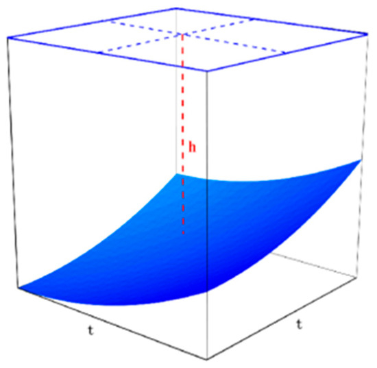
Figure A1.
Schematic diagram of segmentation error.
Therefore, if the selected grid step is shorter, the prediction error will be smaller. However, the resolution of the current gravity anomaly model is insufficient. Regarding the prediction error caused by the selection of different step lengths, this study uses the following simulation experiments to evaluate the accuracy.
The region R is selected as a square sea area of 40 km × 40 km, and four symmetrical conical seamounts are placed directly under R. The radius of the two symmetrical seamounts is 10 km, and the heights are 0.5 km and 1 km, respectively, and they are placed at a depth H of 4 km, as shown in Figure A2a.
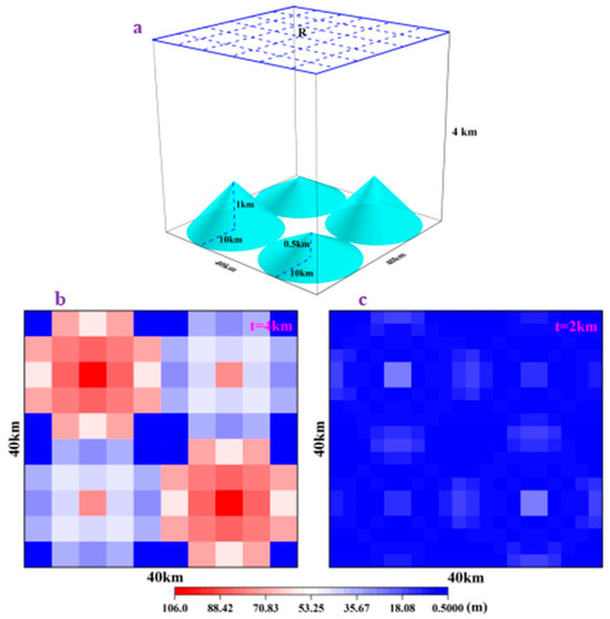
Figure A2.
(a) Schematic diagram of simulated seamount. (b) Inversion error distribution map with 4 km step. (c) Inversion error distribution map with 2 km step.
The VGG anomaly generated by the simulated seamount at the sea level R can be obtained by using the integral formula. Then, choosing two different grid steps of 4 km and 2 km, the depth can be solved iteratively from the observation equation. Figure A2b,c show the error distributions of the prediction results. It can be seen from Figure A2b,c that the error at the center is the largest, the error gradually decreases outward, and the error at the four corners is the smallest. This error characteristic is mainly related to the topographic fluctuations, and the larger the topographic fluctuation, the greater the corresponding error. According to the further statistics, the RMS errors of Figure A2b,c are 56.1 m and 7.2 m, respectively. This shows that the smaller the segmentation step, the smaller the prediction error. That is to say, a more accurate prediction result can be obtained by increasing the resolution of VGG anomalies.
References
- Andersen, O.B.; Knudsen, P. The DTU10 global Mean sea surface and Bathymetry. In Presented EGU-2008; EGU: Vienna, Austria, 2008. [Google Scholar]
- Weatherall, P.; Tozer, B.; Arndt, J.E.; Bazhenova, E.; Bringensparr, C.; Castro, C.; Dorschel, B.; Ferrini, V.; Hehemann, L.; Jakobsson, M.; et al. The GEBCO_2021 Grid—A Continuous Terrain Model of the Global Oceans and Land; British Oceanographic Data Centre NOC: Southampton, UK, 2021. [Google Scholar] [CrossRef]
- Sandwell, D.T.; Smith, W.H.; Gille, S.; Kappel, E.; Jayne, S.; Soofi, K.; Coakley, B.; Géli, L. Bathymetry from space: Rationale and requirements for a new, high-resolution altimetric mission. Comptes Rendus Geosci. 2006, 338, 1049–1062. [Google Scholar] [CrossRef]
- Hwang, C. A Bathymetric Model for the South China Sea from Satellite Altimetry and Depth Data. Mar. Geod. 1999, 22, 37–51. [Google Scholar] [CrossRef]
- Hsiao, Y.S.; Hwang, C.; Cheng, Y.S.; Chen, L.C.; Hsu, H.J.; Tsai, J.H.; Liu, C.L.; Wang, C.C.; Liu, Y.C.; Kao, Y.C. High-resolution depth and coastline over major atolls of South China Sea from satellite altimetry and imagery. Remote Sens. Environ. 2016, 176, 69–83. [Google Scholar] [CrossRef]
- Kim, J.W.; Frese, R.R.B.V.; Lee, B.Y.; Roman, D.R.; Doh, S. Altimetry-derived gravity predictions of bathymetry by gravity-geologic method. Pure Appl. Geophys. 2011, 168, 815–826. [Google Scholar] [CrossRef]
- Ibrahim, A.; Hinze, W.J. Mapping buried bedrock topography with gravity. Groundwater 1972, 10, 18–23. [Google Scholar] [CrossRef]
- Kim, K.B.; Yun, H.S. Satellite-derived Bathymetry Prediction in Shallow Waters Using the Gravity-Geologic Method: A Case Study in the West Sea of Korea. KSCE J. Civ. Eng. 2017, 22, 2560–2568. [Google Scholar] [CrossRef]
- Ramillien, G.; Cazenave, A. Global bathymetry derived from altimeter date of the Ers-1 geodetic mission. J. Geodyn. 1997, 23, 129–149. [Google Scholar] [CrossRef]
- Smith, W.H.F.; Sandwell, D.T. Global sea floor topography from satellite altimetry and ship depth soundings. Science 1977, 277, 1956–1962. [Google Scholar] [CrossRef]
- Kim, K.B.; Hsiao, Y.S.; Kim, J.W.; Lee, B.Y.; Kwon, Y.K.; Kim, C.H. Bathymetry enhancement by altimetry-derived gravity anomaly in the East Sea (Sea of Japan). Mar. Geophys. Res. 2010, 31, 285–298. [Google Scholar] [CrossRef]
- Hwang, C.; Lee, B.Y.; Kim, K.B.; Kim, J.W.; Hsiao, Y.S. Bathymetry estimation using the gravity-geologic method: An investigation of density contrast predicted by the downward continuation method. Terr. Atmos. Ocean. Sci. (TAO) 2011, 22, 347–358. [Google Scholar]
- Hwang, C.; Kao, E.C.; Parson, B. Global derivation of marine gravity anomaly from Seasat, Geosat, ERS-1 and TOPEX/POSEIDON altimeter data. Geophys. J. Int. 1998, 134, 449–459. [Google Scholar] [CrossRef]
- Sandwell, D.T.; McAdoo, D.C. High-accuracy, high-resolution gravity profiles from 2 years of the Geosat exact repeat mission. J. Geophys. Res. Atmos. 1990, 95, 3049–3060. [Google Scholar] [CrossRef]
- Sandwell, D.T.; Smith, W.H.F. Marine gravity anomaly from Geosat and ERS 1 satellite altimetry. J. Geophys. Res. 1997, 105, 10039–10054. [Google Scholar] [CrossRef]
- Armon, M.; Dente, E.; Shmilovitz, Y.; Mushkin, A.; Cohen, T.J.; Morin, E.; Enzel, Y. Determining bathymetry of shallow and ephemeral desert lakes using satellite imagery and altimetry. Geophys. Res. Lett. 2020, 47, e2020GL087367. [Google Scholar] [CrossRef]
- Richard, P.S.; Kristine, H.; Mark, S. Determination of water depth with high-resolution satellite imagery over variable bottom types. Limnol. Oceanogr. 2003, 48, 547–556. [Google Scholar]
- Xu, N.; Ma, X.; Ma, Y.; Zhao, P.; Yang, J.; Wang, X.H. Deriving highly accurate shallow water bathymetry from sentinel-2 and ICESat-2 datasets by a multitemporal stacking method. IEEE J. Sel. Top. Appl. Earth Obs. Remote. Sens. 2021, 14, 6677–6685. [Google Scholar] [CrossRef]
- Caballero, I.; Stumpf, R.P. Towards Routine Mapping of Shallow Bathymetry in Environments with Variable Turbidity: Contribution of Sentinel-2A/B Satellites Mission. Remote. Sens. 2020, 12, 451. [Google Scholar] [CrossRef]
- Li, Y.; Gao, H.; Jasinski, M.F.; Zhang, S.; Stoll, J.D. Deriving High-Resolution Reservoir Bathymetry From ICESat-2 Prototype Photon-Counting Lidar and Landsat Imagery. IEEE Trans. Geosci. Remote. Sens. 2019, 57, 7883–7893. [Google Scholar] [CrossRef]
- Rasheed, S.; Warder, S.C.; Plancherel, Y.; Piggott, M.D. An improved gridded bathymetric data set and tidal model for the maldives archipelago. Earth Space Sci. 2021, 8, e2020EA001207. [Google Scholar] [CrossRef]
- Parker, R.L. The rapid calculation of potential anomaly. Geophys. J. R. Astron. Soc. 1972, 31, 447–455. [Google Scholar] [CrossRef]
- Dixon, T.H.; Naraghi, M.; McNutt, M.K.; Smith, S.M. Bathymetric prediction from SEASAT altimeter data. J. Geophys. Res. Atmos. 1983, 88, 1563–1571. [Google Scholar] [CrossRef]
- Smith, W.H.F.; Sandwell, D.T. Bathymetric prediction from dense satellite altimetry and sparse shipboard bathymetry. J. Geophys. Res. 1994, 99, 803–824. [Google Scholar] [CrossRef]
- Wang, Y.M. Predicting bathymetry from the earth’s gravity gradient anomalies. Mar. Geod. 2000, 23, 251–258. [Google Scholar] [CrossRef]
- Nagy, D.; Papp, G.; Benedek, J. The gravitational potential and its derivatives for the prism. J. Geod. 2000, 74, 552–560. [Google Scholar] [CrossRef]
- Yang, J.J.; Jekeli, C.; Liu, L. Seafloor topography estimation from gravity gradients using simulated annealing. J. Geophys. Res. 2018, 123, 6958–6975. [Google Scholar] [CrossRef]
- Yu, J.; Xu, H.; Wan, X. An analytical method to invert the seabed depth from the vertical gravitational gradient. Mar. Geod. 2021, 44, 306–326. [Google Scholar] [CrossRef]
- Becker, J.J.; Sandwell, D.T.; Smith, W.H.F.; Braud, J.; Binder, B.; Depner, J.; Fabre, D.; Factor, J.; Ingalls, S.; Kim, S.-H.; et al. Global Bathymetry and Elevation Data at 30 Arc Seconds Resolution: SRTM30_PLUS. Mar. Geod. 2009, 32, 355–371. [Google Scholar] [CrossRef]
- Jakobsson, M.; Mayer, L.A.; Bringensparr, C.; Castro, C.F.; Mohammad, R.; Johnson, P.; Ketter, T.; Accettella, D.; Amblas, D.; An, L.; et al. The International Bathymetric Chart of the Arctic Ocean Version 4.0. Sci. Data 2020, 7, 1–14. [Google Scholar] [CrossRef]
- Tozer, B.; Sandwell, D.T.; Smith, W.H.; Olson, C.; Beale, J.R.; Wessel, P. Global bathymetry and topography at 15 arc sec: SRTM15+. Earth Space Sci. 2019, 6, 1847–1864. [Google Scholar] [CrossRef]
- Weatherall, P.; Marks, K.M.; Jakobsson, M.; Schmitt, T.; Tani, S.; Arndt, J.E.; Rovere, M.; Chayes, D.; Ferrini, V.; Wigley, R. A new digital bathymetric model of the world’s oceans. Earth Space Sci. 2015, 2, 331–345. [Google Scholar] [CrossRef]
- Boghosian, A.; Tinto, K.; Cochran, J.R.; Porter, D.; Elieff, S.; Burton, B.L.; Bell, R.E. Resolving bathymetry from airborne gravity along Greenland fjords. J. Geophys. Res. Solid Earth 2015, 120, 8516–8533. [Google Scholar] [CrossRef]
- Fu, L.L.; Alsdorf, D.; Morrow, R.; Rodriguez, E.; Mognard, N. SWOT: The Surface Water and Ocean Topography Mission. 2012. Available online: https://swot.jpl.nasa.gov/system/documents/files/2179_SWOT_MSD_final-3-26-12.pdf (accessed on 18 September 2023).
- Neeck, S.P.; Lindstrom, E.J.; Vaze, P.V.; Fu, L.L. Surface Water and Ocean Topography (SWOT) mission. In Sensors, Systems, and Next-Generation Satellites XVI; SPIE: Washington, DC, USA, 2012. [Google Scholar]
- Mayer, L.; Jakobsson, M.; Allen, G.; Dorschel, B.; Falconer, R.; Ferrini, V.; Lamarche, G.; Snaith, H.; Weatherall, P. The Nippon Foundation—GEBCO Seabed 2030 Project: The Quest to See the World’s Oceans Completely Mapped by 2030. Geosciences 2018, 8, 63. [Google Scholar] [CrossRef]
- Talwani, M. Computer usage in the computation of gravity anomalies. in Geophysics, Methods in Computational Physics: Advances in Research and Applications. Geophysics 1973, 13, 343–389. [Google Scholar]
- Xu, H.; Yu, J. Using an iterative algorithm to predict topography from vertical gravity gradients and ship soundings. Earth Space Sci. 2022, 9, e2022EA002437. [Google Scholar] [CrossRef]
- Sandwell, D.T.; Müller, R.D.; Smith, W.H.F.; Garcia, E.; Francis, R. New global marine gravity model from CryoSat-2 and Jason-1 reveals buried tectonic structure. Science 2014, 346, 65–67. [Google Scholar] [CrossRef] [PubMed]
- Harper, H.; Tozer, B.; Sandwell, D.T.; Hey, R.N. Marine vertical gravity gradients reveal the global distribution and tectonic significance of “seesaw” ridge propagation. J. Geophys. Res. Solid Earth 2021, 126, e2020JB020017. [Google Scholar] [CrossRef]
- Smith, W.H.F. On the accuracy of digital bathymetric data. J. Geophys. Res. 1993, 98, 9591–9603. [Google Scholar] [CrossRef]
- Abulaitijiang, A.; Andersen, O.B.; Sandwell, D. Improved Arctic Ocean bathymetry derived from DTU17 gravity model. Earth Space Sci. 2019, 6, 1336–1347. [Google Scholar] [CrossRef]
- Fan, D.; Li, S.; Meng, S.; Lin, Y.; Xing, Z.; Zhang, C.; Yang, J.; Wan, X.; Qu, Z. Applying Iterative Method to Solving High-Order Terms of Seafloor Topography. Mar. Geod. 2019, 43, 63–85. [Google Scholar] [CrossRef]
- Baudry, N.; Diament, M.; Albouy, Y. Precise location of unsurveyed seamounts in the Austral archipelago area using SEASAT data. Geophys. J. Int. 1987, 89, 869–888. [Google Scholar] [CrossRef]
- Calmant, S.; Baudry, N. Modelling bathymetry by inverting satellite altimetry data:A review. Mar. Geophys. Res. 1995, 18, 123–134. [Google Scholar] [CrossRef]
- Jung, W.Y.; Vogt, P.R. Predicting bathymetry from Geosat-ERM and shipborne profifiles in the South Atlantic Ocean. Tectonophysics 1992, 210, 235–253. [Google Scholar] [CrossRef]
- Watts, A.B.; Sandwell, D.T.; Smith, W.H.F.; Wessel, P. Global gravity, bathymetry, and the distribution of submarine volcanism through space and time. J. Geophys. Res. Solid Earth 2006, 111, B08408. [Google Scholar] [CrossRef]
- McKenzie, D.; Bowin, C. The relationship between bathymetry and gravity in the Atlantic Ocean. J. Geophys. Res. 1976, 81, 1903–1915. [Google Scholar] [CrossRef]
- Sichoix, L.; Bonneville, A. Prediction of bathymetry in French Polynesia constrained by shipboard data. Geophys. Res. Lett. 1996, 23, 2469–2472. [Google Scholar] [CrossRef]
- Hubbert, M.K. A line-integral method of computing the gravimetric effects of two-dimensional masses. Geophysics 1948, 13, 215–225. [Google Scholar] [CrossRef]
- Talwani, M.; Worzel, J.L.; Landisman, M. Rapid gravity computations for two-dimensional bodies with application to the Mendocino submarine fracture zone. J. Geophys. Res. 1959, 64, 49–59. [Google Scholar] [CrossRef]
- Talwani, M.; Ewing, M. Rapid Computation of Gravitational Attraction of Three-Dimensional Bodies of Arbitrary Shape. Geophysics 1960, 25, 203–225. [Google Scholar] [CrossRef]
- Zhdanov, M.S.; Ellis, R.; Mukherjee, S. Three-dimensional regularized focusing inversion of gravity gradient tensor component data. Geophysics 2004, 69, 925–937. [Google Scholar] [CrossRef]
- Martinez, C.; Li, Y.G.; Krahenbuhl, R.; Braga, M.A. 3D inversion of airborne gravity gradiometry data in mineral exploration: A case study in the Quadrilátero Ferrífero, Brazil. Geophysics 2013, 78, B1–B11. [Google Scholar] [CrossRef]
- Geng, M.; Huang, D.N.; Yang, Q.J.; Liu, Y.P. 3D inversion of airborne gravity-gradiometry data using cokriging. Geophysics 2014, 79, G37–G47. [Google Scholar] [CrossRef]
- Qin, P.B.; Huang, D.N. Integrated gravity and gravity gradient data focusing inversion. Chin. J. Geophys. 2016, 56, 2203–2224. (In Chinese) [Google Scholar]
- Pavlis, N.K.; Holmes, S.A.; Kenyon, S.C.; Factor, J.K. An Earth gravitational model to degree 2160: EGM2008. In Proceedings of the 2008 General Assembly of the European Geosciences Union, Vienna, Austria, 13–18 April 2008. [Google Scholar]
- Huan, X.; Jinhai, Y.; Xiaoyun, W.; Lei, L. An expression for gravity generated by an anomalous geological body and its application in bathymetry inversion. J. Geod. Geoinf. Sci. 2021, 4, 63–73. [Google Scholar] [CrossRef]
- Sandwell, D.T.; Goff, J.A.; Gevorgian, J.; Harper, H.; Kim, S.; Yu, Y.; Tozer, B.; Wessel, P.; Smith, W.H.F. Improved Bathymetric Prediction Using Geological Information: SYNBATH. Earth Space Sci. 2022, 9, e2021EA00206. [Google Scholar] [CrossRef]
- Morrow, R.; Fu, L.-L.; Ardhuin, F.; Benkiran, M.; Chapron, B.; Cosme, E.; D’ovidio, F.; Farrar, J.T.; Gille, S.T.; Lapeyre, G.; et al. Global Observations of Fine-Scale Ocean Surface Topography With the Surface Water and Ocean Topography (SWOT) Mission. Front. Mar. Sci. 2019, 6, 232. [Google Scholar] [CrossRef]
- Yu, D.; Hwang, C.; Andersen, O.B.; Chang, E.T.; Gaultier, L. Gravity recovery from SWOT altimetry using geoid height and geoid gradient. Remote. Sens. Environ. 2021, 265, 112650. [Google Scholar] [CrossRef]
- Liu, P.; Wang, M.; Wang, L.; Han, W. Remote-Sensing Image Denoising With Multi-Sourced Information. IEEE J. Sel. Top. Appl. Earth Obs. Remote. Sens. 2019, 12, 660–674. [Google Scholar] [CrossRef]
- Wang, P.; Wang, L.; Leung, H.; Zhang, G. Super-Resolution Mapping Based on Spatial–Spectral Correlation for Spectral Imagery. IEEE Trans. Geosci. Remote. Sens. 2020, 59, 2256–2268. [Google Scholar] [CrossRef]
Disclaimer/Publisher’s Note: The statements, opinions and data contained in all publications are solely those of the individual author(s) and contributor(s) and not of MDPI and/or the editor(s). MDPI and/or the editor(s) disclaim responsibility for any injury to people or property resulting from any ideas, methods, instructions or products referred to in the content. |
© 2023 by the authors. Licensee MDPI, Basel, Switzerland. This article is an open access article distributed under the terms and conditions of the Creative Commons Attribution (CC BY) license (https://creativecommons.org/licenses/by/4.0/).