Abstract
To address the issue of integrity monitoring for a multi-source information fusion navigation system, a theoretical framework of two-level integrity monitoring is proposed. Firstly, at the system level, a system-integrity-monitoring method based on the Kalman filter weighted least-squares form is established to detect and isolate faulty navigation sources. Secondly, at the sensor level, considering the redundancy of the faulty navigation sources, this paper presents the design of a multi-mode comprehensive fault-detection method for non-redundant navigation sources. Additionally, an extended-dimension matrix optimized sensor-fault detection and verification method for redundant navigation sources is proposed. Finally, integrity risk allocation criteria are established based on the effectiveness of navigation sources to calculate the system protection level and trigger integrity alarms. The two-level integrity-monitoring method was tested on a multi-source information fusion navigation system integrated with an inertial navigation system (INS), global positioning system (GPS), BeiDou satellite navigation system (BDS), Doppler velocity log (DVL), barometric altimeter (BA), and terrain-aided navigation (TAN). Test results demonstrate that the proposed method can effectively isolate the faulty navigation source within 10 s. Furthermore, it can detect the faulty sensors within the faulty navigation sources, thereby enhancing the reliability and robustness of the multi-source information fusion navigation system.
1. Introduction
With the introduction and promotion of the “all source navigation” concept, the navigation system is progressively evolving towards diversifying navigation sources, expanding compatibility, and adopting the plug-and-play approach. In routine operational conditions, a multi-source information fusion navigation system, equipped with a substantial number of redundant navigation observations, can deliver high-precision, highly reliable, and interference-resistant navigation services for the carrier. However, in practical applications, various factors such as adverse environmental conditions, human interference, and hardware aging can contribute to the potential failure of any navigation source. If these faults are not promptly detected, the entire navigation system may be compromised by erroneous data, resulting in a reduction in navigation accuracy. In severe cases, such failures can lead to overall breakdown of the navigation system [1,2]. Therefore, establishing an integrity-monitoring method for a multi-source information fusion navigation system is a crucial issue that requires resolution.
Integrity monitoring of navigation systems is crucial for ensuring confidence in positional information, encompassing the system’s ability to promptly alert users when navigation becomes unreliable [3,4]. Early integrity monitoring predominantly targets homogeneous and redundant navigation sources within the global navigation satellite system (GNSS), capable of detecting abnormalities in satellite measurements, receiver hardware, or signal distortions. A widely adopted method is receiver autonomous integrity monitoring (RAIM) [5,6,7]. In recent years, numerous scholars have enhanced and innovated RAIM algorithms. For instance, in reference [8], an integrity-monitoring algorithm is proposed, utilizing the innovation variance of the Kalman filter for fault detection (KF-RAIM). Reference [9] achieved integrity monitoring based on carrier phase observation (CRAIM). Reference [10] introduces an advanced RAIM algorithm (ARAIM) that ensures both horizontal and vertical integrity requirements. Addressing the issue of data delay, reference [11] proposes a relative RAIM algorithm (RRAIM). Furthermore, to account for time variability, reference [12] introduces a time-RAIM algorithm (TRAIM). However, these algorithms are all designed for homogeneous and redundantly equipped GNSS navigation sources. In contrast, non-redundant multi-sensor navigation sources, such as terrain-aided navigation (TAN), have relatively few associated integrity algorithms. For instance, references [13,14,15] propose a terrain-data anomaly detection algorithm based on GPS and radar altimeters. This method involves horizontal consistency detection by estimating and extracting terrain heights, introducing positive and negative vertical deviations on the measured elevation, and stacking horizontal detection results layer by layer to form a spatial envelope. However, this approach heavily relies on the precise positional information provided by satellite navigation systems. The key challenge lies in monitoring terrain data and height-sensor anomalies in the event of a satellite navigation system failure and avoiding mismatches, which is crucial for ensuring the integrity of TAN.
Currently, the focus of integrity monitoring for multi-source information fusion navigation systems is primarily on GNSS/INS fusion navigation systems, with many algorithms still relying on GNSS integrity-monitoring methods. For instance, reference [16] effectively detects slowly increasing errors in satellites by extrapolating and accumulating new information from multiple epochs of the GNSS/INS integrated navigation system. References [17,18,19] employ the least-squares multiple solution separation method to detect faults in navigation sources. However, when constructing the least-squares separation solution in the location domain, the measurement error can be easily submerged, leading to low sensitivity in small-fault detection. References [20,21,22] utilize federated filters to create multiple binary sub-filters and employ fuzzy logic and weighted residual eigenvalues for each sub-filter to achieve fault diagnosis. Although this method can detect and isolate faulty navigation sources, its primary goal is to enhance the system’s fault tolerance and it cannot calculate the system protection level. Additionally, as the number of fused navigation sources increases, the need to establish sub-filters also significantly increases. References [23,24,25,26] proposes a multi-sensor integrity-management model that accomplishes integrity management of multiple sensors by dynamically assigning each sensor to one of four modes: monitoring, validation, calibration, and reconstruction. Although the model has a relatively complete logical structure, as the number of sensors and simultaneously faulty sensors increases, the number of parallel sub-filters that need to be constructed significantly increases, resulting in an escalation of computational load.
In summary, research on integrity-monitoring methods for multi-source information fusion navigation systems is still in its early stages, and the detection of faults in navigation systems is currently limited to a single hierarchical structure of navigation sources or sensors. However, multi-source information fusion navigation systems feature a redundant configuration structure. The impact of sensor faults in a particular navigation source on the entire navigation system exhibits significant hierarchical transmission characteristics. Additionally, diverse types of information sources, varying dimensions of measurement matrices, and distinct characteristics of measurement noise in multi-source information fusion navigation systems present new challenges to integrity monitoring.
In this paper, we propose a two-level integrity method for multi-source information fusion navigation; the structure is shown in Figure 1. This method can detect, isolate, and verify faulty navigation sources and faulty sensors at different levels, and dynamically adjust the fault hypotheses that need to be monitored to calculate the system protection level, so as to realize the integrity monitoring of multi-source information fusion navigation.
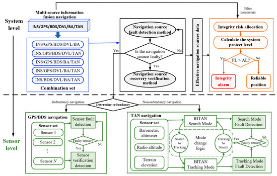
Figure 1.
The two-level integrity monitoring structure.
In detail, the contributions of this paper are as follows:
- (1)
- A two-level integrity-monitoring structure is introduced. Utilizing the loosely coupled filtering model, the structure establishes integrity-monitoring models at both the system and sensor levels. It accomplishes fault detection, isolation, and verification from navigation sources to sensors in a systematic manner.
- (2)
- For the navigation source TAN, based on its working principle, this paper designs search-mode and tracking-mode fault-detection models to achieve integrity monitoring for non-redundant navigation sources.
- (3)
- The proposed integrity-monitoring method adopts the integrity risk dynamic allocation criterion, allowing the dynamic adjustment of monitored fault hypotheses based on the effective navigation sources in the system.
The remainder of this paper is structured as follows. Section 1 introduces the current research status of navigation integrity monitoring. Section 2 elaborates on the system-level integrity-monitoring method. Section 3 focuses on the fault detection methods for two types of navigation sources at the sensor level. Section 4 introduces the integrity risk allocation criteria and protection-level calculation. Section 5 presents the simulation test results of the proposed method. Finally, concluding remarks and future research directions are provided in Section 6.
2. System-Level Integrity-Monitoring Method
At system level, a loosely coupled filtering model is constructed for each navigation source. Therefore, it is necessary to design a fault-detection model to detect and isolate faulty navigation sources. Meanwhile, to ensure fault-detection capability, this paper presents the design of a navigation source recovery verification model to judge whether the isolated navigation source has returned to normal.
2.1. Navigation-Source Fault-Detection Model
Differing from the traditional multiple-solution separation method in the position domain [27], we have designed a multiple residual separation method in the measurement domain.
Since three sets of inertial navigation systems are typically employed in airborne applications to ensure the reliability of inertial navigation, INS faults are not considered in this paper. Subsequently, the remaining navigation sources are ranked to form different combinations. Assuming that the number of simultaneous faulty navigation sources is one, the fusion navigation system INS/GPS/BDS/DVL/BA/TAN has the following five forms of combinations:
Combination 1 (Com1): INS/GPS/BDS/DVL/BA
Combination 2 (Com2): INS/GPS/BDS/DVL/TAN
Combination 3 (Com3): INS/GPS/BDS/BA/TAN
Combination 4 (Com4): INS/GPS/DVL/BA/TAN
Combination 5 (Com5): INS/BDS/DVL/BA/TAN
where represents the position difference between navigation source and INS, represents the velocity difference between the navigation source and INS, represents the altitude difference between BA and INS.
The traditional extended Kalman filter (EKF) [28] mainly comprises two components: state propagation and measurement update. The updated state estimation results from the combined influence of historical states and current measurements. This introduces the possibility of the integrity risk being related to past states. Furthermore, the Kalman filter gain acts as a time-varying matrix, exacerbating the correlation between the two. Therefore, it is essential to establish a direct mapping relationship between the final state and the input. Additionally, the measurement update formula in the classical EKF should be reconstructed into a least-squares form [19], encompassing both system propagation and measurement, as illustrated below:
where k is the time epoch, is a 15-dimensional system state, is the one-step state prediction obtained through the Kalman filter, is the measurement matrix of the Kalman filter, is the noise matrix with the corresponding covariance matrix , as follows:
Yk = CkXk + vzx
Using as the weight matrix, the state estimation solution of Kalman filter weighted least-squares form is:
By setting the partial elements of the weight matrix to zero (the navigation source in which combination c is not contained), the separation residual with covariance matrix of combination c is obtained as follows:
where is the all-measurement vector, is the separation solution, is the weight matrix, is the noise covariance matrix.
The fault detection statistic of combination c is constructed from the Mahalanobis distance of the separation residual, satisfies the chi-square distribution with n degrees of freedom, and its corresponding threshold is calculated as follows:
where is the significance level, which is the probability of integrity risk assigned to the subsystem, represents the chi-square probability distribution function, n is the measurement dimension.
The faulty navigation source can be isolated based on the relationship between and under each combination. For the INS/GPS/BDS/DVL/BA/TAN navigation, the detection results under different fault cases are shown in Table 1, where 1 represents and 0 represents .

Table 1.
The Detection Results under Different Fault Cases.
2.2. Navigation-Source Fault-Detection Model
Previously faulty navigation sources that have returned to normal, such as isolated faulty sensors, can be reintegrated into the fusion positioning solution. However, before re-inclusion, recovery verification is necessary to prevent contaminating the fusion solution.
A least-squares form is constructed that includes measurement information provided by the KF main system state and isolated navigation sources, as follows:
where is the untrusted measurement, is the measurement noise variance matrix, is the measurement matrix, is the estimated state provided by the main filter, is the state error covariance matrix.
This paper uses the w-detection method [29] for verification. If there are multiple navigation source to be verified, parallel verification can be carried out. Therefore, the validation detection statistics and detection thresholds in the least-squares form are:
where ei is the vector with the i-th element (untrusted measurement) 1, and the remaining elements are 0, Pzz is the measurement residual covariance matrix in the LS form, ∇Si represents the critical outlier.
According to Formulas (15) and (16), real-time verification can be performed on isolated navigation sources. If the verification detection is less than the detection threshold five consecutive times, it is judged that the isolated navigation source has returned to normal.
3. Sensor-Level Integrity-Monitoring Method
For non-redundant navigation source systems, isolating a faulty sensor will render the navigation source inoperable. However, a hardware reset or a “heartbeat” reset can be performed on a faulty sensor to restart the navigation source. In the case of redundant navigation sources, they can continue to function normally even after isolating faulty sensors.
3.1. Non-Redundant Navigation Source TAN
Terrain-aided navigation utilizes airborne terrain-elevation databases, barometric altimeters, and radio altimeters to achieve multi-sensor, non-redundant, and heterogeneous fusion navigation. Various TAN algorithms exist, and this paper primarily investigates the integrity monitoring method of the robust BITAN algorithm [30]. The BITAN algorithm encompasses two working modes: search and tracking. Consequently, this paper presents the design of a multi-mode comprehensive fault-detection method.
3.1.1. Search-Mode Fault-Detection Model
From the moment that the system enters the search mode until the epoch that fulfills the search conversion logic, the terrain data at each search location are tallied to compute the sum of the squares of the absolute deviation of the Mahalanobis distance. The fault statistics for the search mode are established as:
where is the number of the time epoch that satisfies the search conversion logic, is the estimated terrain data obtained by barometric altimeter and radio altimeter at time , represents the terrain data in row and column within the search scope, is the standard deviation of absolute deviation error.
The threshold of the search-fault-detection statistic can be obtained by preset probability of false detection, and the value at each position in the search range is compared. Therefore, the search anomaly for the missed detection identifier is as follows. Mapping the to the search area can obtain the abnormal missed detection area :
The search mode is prone to mismatches in the following three situations: (1) When the search filtering position is located outside the abnormal search missed detection area. (2) When the deviation between the search filtering position and the minimum position in is significant. (3) When the area of the missed area in the search for abnormal missed areas is relatively large.
Therefore, through a comprehensive search of the abnormal missed detection area and minimizing position deviation, the design for determining anomalies in the search positioning results is as follows:
where and are the deviations between the minimum position and the search filtering position, is the deviation threshold, represents the maximum value, represents the minimum value, is the proportion of missed detection area, is the threshold for the proportion of missed detection area, indicates that the search is normal, indicates an abnormal search, and needs to be re-searched and filtered.
3.1.2. Tracking-Mode Fault-Detection Model
The measurement residual of the tracking filter is used to construct the fault-detection statistic as follows:
where is the k-th time epoch, represents the measured value, is the measurement matrix, is the estimated state value, is the covariance matrix of state error, is the covariance matrix of measurement noise.
Under fault-free conditions, the tracking anomaly detection statistic follows a central chi-square distribution; under fault conditions, it follows a non-central chi-square distribution. Based on the prior probability of false detection and the measurement of degrees of freedom, the threshold for tracking-fault-detection statistics can be obtained. When Tt is greater than Ttd, there is a fault in the tracking mode, and the system will switch back to search mode.
3.2. Redundant Navigation Source GPS/BDS
3.2.1. Sensor-Fault Detection Model
The redundant navigation source comprises multiple homogeneous sensors. For the fault detection of these sensors, the parallel sub-filter method proposed by Jurado J. D. is effective in identifying faulty sensors. The working principle of this method is summarized as follows: the method firstly creates parallel sub-filters by excluding one sensor measurement in turn. Secondly, it constructs a sliding-window residual Mahalanobis distance as the fault-detection statistics for each sensor in each sub-filter. Then, based on the fault-detection results for each sensor in each sub-filter, the method designs a score vector to sum the fault-detection results of all sensors in each sub-filter. Finally, when there is a unique non-zero value in the score vector, the sensor excluded by the sub-filter corresponding to that non-zero value is the faulty sensor. However, this method presents a delay issue in detecting faults across multiple sensors. Therefore, this paper introduces an expanded-dimension matrix optimization method to enhance multi-fault-detection performance. The design and construction of sensor-fault detection statistics are detailed in reference [23]. In this paper, our focus is on elucidating the construction process of the expanded-dimension matrix.
When the sensor level detects multiple faults or identifies faulty sensors, it becomes necessary to reinitialize and construct a new parallel sub-filter. This process requires a specific sampling interval for the initialized detection model to identify the corresponding fault. However, detection delays may result in undetected fault sensors affecting the accuracy of the navigation solution, and in severe cases, may lead to filtering divergence. This paper addresses these issues by establishing the corresponding relationship between the old sub-filters and new sub-filters to construct the expanded dimension. Subsequently, the new fault-detection statistics are initialized for each sub-filter.
For each old sub-filter, excluding one sensor at a time can yield multiple sensor combinations, forming the expanded dimension. Interestingly, we observe that these combinations are identical to the sensor combinations in the new sub-filter. Consequently, the fault-detection statistics with the same sensor combinations in the expanded dimension are averaged. These averaged values are then assigned to the new sub-filters as initial values. This approach effectively mitigates the impact of adjusting the number of simultaneous faults on the fault-detection time. The calculation formula for the extended-dimension matrix and the new fault-detection statistics is as follows:
where is the number of simultaneous faults in the old sub-filter, is the number of simultaneous faults in the new sub-filter, is the new sub-filter serial number, is the sensor combination in extended-dimension matrix , is the sensor combination of the j-th new sub-filter.
When the extended-dimension matrix detects multiple faults, the reconstructed parallel sub-filter is initialized. Additionally, for the adjustment of the parallel sub-filter after isolating faulty sensors or adding new sensors (after verification), an extended-dimension matrix can also be used for optimized assignment.
3.2.2. Sensor-Recovery Verification Model
The verification filter model is essentially similar to the navigation source filter solution model, with the difference lying in the measurement model. The validation measurement model is constructed from both untrusted sensor measurements and normal sensor measurements within the navigation source. The measurement model is:
where vaild represents the normal sensor, represents the untrusted sensor to be verified.
The validation test statistics are calculated from the measurement residuals of the untrusted sensors during the validation period as follows:
where Rk,v is the covariance matrix of the measurement noise, is the state estimation provided by the verification filter, Pk is the state error covariance matrix, Mv is the verification period.
If the verification detection is below the threshold, the sensor is deemed credible and can be reintegrated into the navigation source solution. Otherwise, the sensor is considered untrusted. Furthermore, when successfully validated sensors are reintroduced into the navigation source solution, it is necessary to adjust the sensor-fault-detection model using the extended-dimension matrix.
4. System-Protection-Level Calculation
4.1. Integrity Risk Allocation Criteria
It is well known that any fault-detection model has a missed-detection probability. In a navigation system, integrity risk is typically defined as the probability that the position error (PE) exceeds the alert limit (AL) and the fault is not detected. To ensure the reliability of the navigation system, the probability that the PE exceeds the AL and the fault is not detected must be less than or equal to the integrity risk probability budget Prisk. The relationship between the integrity risk and the position error [31] can be defined as:
where is the fault detection statistics and is the detection threshold.
For a multi-source information fusion navigation system, the integrity risk can be expressed as the multiple-fault hypothesis. Let represent the fault hypothesis and be the fault-free hypothesis. For each fault hypothesis, its integrity risk can be expressed as:
Because, in practical applications, the true error of the system is unknown but the probability of integrity risk can be budgeted based on carrier requirements, therefore, the ultimate goal of integrity monitoring is to derive the position error bound, commonly known as the protection level (PL), through the integrity risk budget. Subsequently, an integrity alert is sent when the PL exceeds the AL. Therefore, Equation (27) can be further rewritten as:
In a multi-source information navigation system, the prior probability of the occurrence of certain fault hypotheses is lower than the required integrity risk. These fault hypotheses do not need to be monitored. Let be the minimum number of fault hypothesis that need monitoring. The fault hypotheses can be categorized into two classes. One includes the fault hypotheses exceeding (labeled as ). The other comprises the remaining fault hypotheses that need monitoring. The system integrity risk is:
where is the total prior probability of occurrence of fault hypotheses that need not be monitored.
For satellite navigation systems, the ARAIM algorithm report provides a clear value for the integrity risk probability budget, with the prior fault probability of each satellite being equal. However, in a multi-source information fusion navigation system, the prior fault probability of each navigation source is not uniform, and there is no clear definition for the prior fault probability of each navigation source. According to existing research [32], the prior failure probability of GPS and BDS navigation sources is set to , DVL to , BA to , and TAN to . Without considering INS fault, the maximum value of the fault hypothesis is when the TAN is updated and when the TAN is not updated. Therefore, under different fault hypotheses, the system’s ability to meet the integrity risk probability also varies. It is essential to dynamically adjust the fault hypotheses that need monitoring based on the actual effective participation of navigation sources.
For airborne multi-source information fusion navigation systems, the overall integrity risk of the system is set to , in the horizontal direction, and in the vertical direction. For the convenience of observing the satisfaction of integrity risk under different fault assumptions, the logarithmic ratio of the integrity risk level is calculated as:
The logarithm of integrity risks under different fault hypotheses was calculated, as shown in Figure 2a. In Figure 2a, the black dashed line represents the situation when the prior fault probability is assumed to be equal to the integrity risk. A ratio less than 1 indicates that the probability of fault assumption occurrence is greater than the integrity risk, while a ratio greater than 1 indicates that the probability of fault assumption occurrence is less than the integrity risk. Therefore, for the multi-source information fusion navigation system INS/GPS/BDS/DVL/BA/TAN, regardless of whether the TAN system is updated or not, the fault assumptions that need to be monitored are all less than .
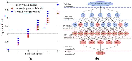
Figure 2.
Schematic diagram of integrity risk allocation. (a) Logarithmic ratio of integrity risk; (b) dynamic monitoring tree for integrity risk.
Additionally, not all combinations of fault hypothesis need to be monitored, and the combinations that require monitoring will also change in real time based on the effective navigation source in the system. Therefore, to facilitate the monitoring of navigation source combinations under different fault hypothesis, this paper establishes a dynamic monitoring tree for integrity risk to monitor fault hypotheses and combinations.
For the INS/GPS/BDS/DVL/BA/TAN system, the integrity risk dynamic monitoring tree under the updated TAN conditions is illustrated in Figure 2b, where the red represents combinations that do not need to be monitored, and the blue represents combinations that need to be monitored. Here, G denotes GPS, B denotes BDS, D denotes DVL, A denotes BA, and T denotes TAN.
4.2. Protection Level Calculation
We derived the protection level under the least-squares method in our previous work [33]. Here, we provide the final protection-level calculation formula as follows:
where is the fault-detection threshold, is the risk factor calculated according to the probability of missed detection, is the standard deviation of position estimation error, is the projection slope from the measurement domain to the positional domain, obtained by the ratio of the square of the mean state error of the fault vector to the non-central parameter of the measurement residual.
where fk is the fault vector, is the pseudo inverse of the observation matrix , .
For each fault hypothesis , there are several combinations that need to be monitored, and the protection levels calculated for each combination reflect the position error. To obtain a more conservative protection limit, the maximum value is selected. Therefore, the protection level under fault hypothesis is:
By combining Formulas (30) and (32), the integrity risk of multi-source information fusion navigation systems can be further expressed as:
where is the protection level under the fault-free hypothesis, and are the standard deviation of estimated position error under the fault-free hypothesis and fault hypothesis, respectively, is the maximum projection slope under the fault hypothesis, is the fault-detection threshold.
The PL can be obtained by solving Equation (36), but solving the above inequality exactly is a complex process. This paper employs the half-interval search method proposed in the ARAIM baseline algorithm to calculate the protection level. The detailed steps of the half-interval search method have been previously described [34,35].
5. Results and Analysis
Using a simulated flight trajectory and real terrain-elevation data (with a resolution of 30 m), the proposed method was tested and validated by constructing a simulated airborne multi-source information fusion navigation system INS/GPS/BDS/DVL/BA/TAN. The specific simulation parameters are shown in Table 2. For the various navigation sources, the respective update periods were set as shown in Table 3.
Table 2.
Simulation Parameter Settings.
Table 3.
Update Period of Different Navigation Sources.
Constant deviation faults and slowly increasing faults were added to the sensor measurements of different navigation sources at different time epochs to construct fault cases and verify the fault-detection ability of the proposed method. The specific fault description is shown in Table 4, where RA represents radio altitude, Vn represents north velocity, SAT represents satellite, GIF represents gradual increase fault, and CBF represents constant bias fault.
Table 4.
Simulation Fault Description.
5.1. Performance of System-Level Integrity Monitoring
This paper analyzes the system-level navigation-fault-detection results under different fault cases without activating sensor-level integrity monitoring, as shown in Table 5. The results include the fault-detection time Tdec, and the RMSE values without fault isolation (FI) and with FI. Using Case 1 and Case 5 as examples, the results of system-level integrity monitoring are illustrated in Figure 3 and Figure 4, respectively. In the fault-detection statistics curve, the upper part represents the result without FI, while the lower part represents the result with FI.
Table 5.
System-Level Fault-Detection Results.
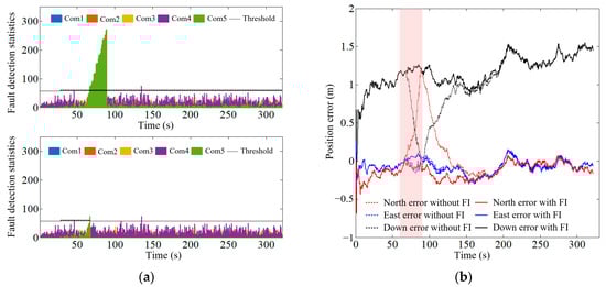
Figure 3.
System-level integrity-monitoring results in Case 1. (a) Fault-detection statistics curve; (b) position error curve.
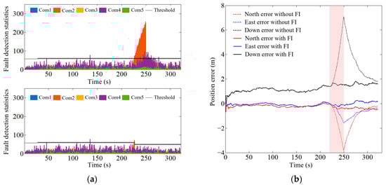
Figure 4.
System-level integrity-monitoring results in Case 5. (a) Fault-detection statistics curve; (b) position error curve.
It can be seen from Figure 3a and Figure 4a that the detection statistics without FI for Com5 and Com2 significantly exceed the threshold, while the fault-detection statistics with FI are less than the threshold. This indicates that the fault-detection model design proposed in this paper can effectively detect the faulty navigation source. Comparing the position error curves without FI and with FI, it can be seen that if the fault is not isolated, the position error curve changes significantly, as shown in the red area in Figure 3b and Figure 4b.
From Table 5, it can be seen that in Case 1, the RMSE values without FI were 0.12 m, 0.28 m, and 1.09 m in the east, north, and down directions, respectively. The RMSE values with FI were 0.11 m, 0.17 m, and 1.18 m in the east, north, and down directions, respectively. Compared with the RMSE values without FI, the RMSE values with FI decreased by 0.01 m and 0.11 m in the east and north directions, respectively, while the RMSE values in the down direction increased by 0.09 m. It can be seen from Figure 3a that under normal conditions, the initial down error was positive. After adding faults, the down error increased in the negative direction, leading to a decrease in the RMSE value. The same situation also occurred in Case 2. For Case 3 to Case 5, taking the east direction as an example, compared with the RMSE without FI, the RMSE values with FI decreased by 0.02 m, 2 m, and 0.35 m, respectively. In addition, from the detection time of the navigation source fault shown in Table 5, it can be seen that for constant deviation and slowly increasing faults, the system-level integrity-monitoring model can detect and isolate the navigation source fault within 6 s.
Taking Case1 to Case3 as examples, the RMSE values with and without navigation source recovery validation function (NRV) are shown in Table 6, including the verification success time Tval.
Table 6.
Navigation Source Recovery Verification Results.
From Table 6, taking the north direction as an example, the RMSE values without the NRV function are 0.17 m, 0.19 m, and 0.16 m in Case 1, Case 2, and Case 3, respectively. The RMSE values with the NRV function are 0.16 m, 0.17 m, and 0.13 m in Case 1, Case 2, and Case 3, respectively. Compared with the RMSE values without NRV function, the RMSE values with the NRV function decreased by 0.01 m, 0.02 m, and 0.03 m in Case 1, Case 2, and Case 3, respectively, indicating a slight improvement in positioning performance.
To further verify the advantages of the method proposed in this paper, based on the faults set in Table 4 (reducing the amplitude of each fault), the multi-combination separation residual method proposed in this paper and the multi-solution separation method proposed in reference [19] were used for navigation-source fault detection. The fault-detection time under different methods is shown in Table 7.
Table 7.
The fault-detection time under different methods.
It can be seen from Table 7, even with reduced fault amplitude, our method can still detect the navigation source faults under five cases, while the method of reference [19] can detect only the BA, DVL, and BDS faults, and missed detecting the TAN and GPS faults. In addition, in the fault cases, both methods can detect navigation-source faults; the detection time of the proposed method is 5 s, 0.5 s and 1.5 s faster than the detection time of the method proposed in reference [19]. Therefore, compared with the multi-solution separation method, the multi-combination separation method has higher sensitivity in fault detection.
5.2. Performance of Sensor-Level Integrity Monitoring
5.2.1. Non-Redundant Navigation Source TAN
The integrity-monitoring method for non-redundant navigation sources TAN, as proposed in this paper, was tested and validated under various working modes of the BITAN algorithm.
(1) Search-mode fault detection (SMFD)
In the search mode of terrain-aided navigation, a faulty sensor is often constrained by the search conversion logic, preventing the system from transitioning to the tracking mode. During such instances, the fault does not pose an integrity risk to the system. However, when the anomaly precisely aligns with the conversion requirements, the provided matching position can significantly deviate from the actual position, impacting the overall positioning performance. Additionally, an incorrect matching position may occur due to the influence of search filtering parameters, if the preset filtering measurement noise variance matrix R parameter is not appropriate. To test and verify the search-mode fault-detection model, this paper described the introduction of anomalies in sensor data and search filtering parameters, creating search anomaly cases. The description of anomaly test cases is presented in Table 8. Table 9 displays the RMSE values of TAN with and without SMFD for different cases. The SMFD results under abnormal search Case 2 are depicted in Figure 5, with the missed detection area highlighted in the red area in Figure 5b.
Table 8.
Description of Abnormal Search Cases.
Table 9.
The RMSE with and without SMFD.
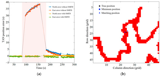
Figure 5.
The SMFD results under abnormal search Case 2. (a) Position error curve; (b) missed detection area.
From Figure 5, it is evident that when a significant deviation occurs between the matching position provided by the search mode and the true value, the search-mode fault-detection model designed in this paper can effectively identify anomalies and reinitialize the search filter. Without SMFD, the TAN performs the tracking filtering based on mismatching positions, leading to incorrect positional information. Table 9 provides an example using north error, revealing that compared with RMSE values of TAN without SMFD, the RMSE values of TAN with SMFD decreased by 36.17 m, 35.16 m, and 107.53 m, respectively. Therefore, the SMFD model proposed in this paper can effectively prevent mismatching, thereby enhancing the reliability of TAN.
(2) Tracking-mode Fault detection (TMFD)
For the tracking mode, as it utilizes single-state Kalman filtering based on height measurement values, a failure in the radio altimeter sensor or barometric altimeter sensor directly impacts the positioning performance. The proposed TMFD model was tested using Case 1 and Case 2 from Table 4. Table 10 displays the fault-detection time and RMSE values for TAN with and without TMFD. Figure 6 illustrates the TMFD results under Case 1, where the fault-detection statistics curve in Figure 6a shows the upper part as the result without TMFD and the lower part as the result with TMFD.
Table 10.
The RMSE with and without TMFD.
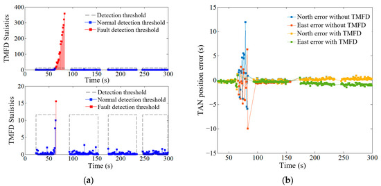
Figure 6.
The TMFD results under Case 1. (a) Fault-detection statistics curve; (b) position error curve.
From Figure 6, it is evident that the tracking-mode fault-detection model proposed in this paper can effectively identify anomalies in the height sensor and promptly switch back to the search mode. Moreover, Table 10 demonstrates a significant reduction in position error with TMFD. Taking the east error as an example, under Case 1 and Case 2, the position error with TMFD decreased by 1.24 m and 0.78 m, respectively, effectively ensuring the reliability of TAN positioning.
5.2.2. Redundant Navigation Source GPS/BDS
Using Case 4 and Case 5 in Table 4 to test the navigation source redundancy integrity-monitoring method, the results of sensor-fault-detection and verification are presented in Table 11. The RMSE value with and without sensor fault isolation (SFI) are provided in Table 12. The navigation source position error curves with and without SFI are plotted as shown in Figure 7.
Table 11.
The Results of Sensor Fault Detection and Verification.
Table 12.
The RMSE without and with SFI.
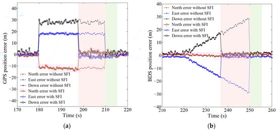
Figure 7.
The navigation source position error curve. (a) GPS navigation; (b) BDS navigation.
It can be observed from Figure 7 and Table 12 that the sensor fault detection and validation model can enhance the positioning accuracy of the navigation source. Taking the GPS navigation source as an example, the RMSE values of GPS without SFI were 5.57 m, 3.74 m, and 8.87 m in the north, east, and down directions, while the RMSE values with SFI were 4.35 m, 3.00 m, and 7.02 m. In comparison to the RMSE values of GPS without SFI, the RMSE values with SFI decreased by 1.22 m, 0.74 m, and 1.85 m, respectively. The sensor integrity monitoring can enhance the positioning accuracy of navigation sources while ensuring the positioning reliability of the multi-source information fusion navigation system.
In addition, sensor integrity monitoring can significantly reduce the duration of navigation source failures, as depicted by the red areas in Figure 7. According to Table 11, the original recovery time of GPS simulation failures was 210 s, and the recognition time for sensor failures was 198 s. By isolating the faulty sensor, the recovery time of the navigation source was reduced by 12 s. The original recovery time of BDS simulation faults was 250 s, and the recognition time for sensor faults was 236.5 s. By isolating the faulty sensor, the recovery time of the navigation source was reduced by 13.5 s. The sensor verification function can rapidly recover the isolated sensor after the fault disappears, as shown in the green areas in Figure 7. The verification success time of the GPS faulty sensor was 215 s, and the verification success time of the BDS faulty sensor was 256 s. Compared with the original recovery time of the simulated faults, the two examples went through verification cycles of 5 s and 6 s, respectively, after the fault disappeared, and the isolated sensor could be reintegrated into the navigation source solution. The corresponding positioning accuracy was restored to the level before the fault.
To verify the performance of the extended-dimension matrix optimization method proposed in this paper, the fault-detection results of the original method and the optimized method were calculated for Case 4, as shown in Table 13, where Tsdec represents the sensor fault detection time and Tsvar represents the sensor verification success time.
Table 13.
The Sensor Fault Detection Results of the Original Method and Optimized Method.
From the fault detection and verification results in Table 13, it can be seen that the original method identified the faulty sensors in 10.5 s, while the optimized method identified the faulty sensors in 7.5 s. Compared with the original method, the optimized method was able to identify faulty sensors faster, and the fault identification time was shortened by 3 s. The sensor validation success time of the original method was 5.5 s, and the sensor validation success time of the optimized method was 5 s. The validation success times of the two methods were basically the same. The RMSE of GPS for the original method was 4.63 m, 3.19 m, and 7.46 m, while the RMSE of GPS for the optimized method was 4.35 m, 3.00 m, and 7.02 m. Compared with the original method, the RMSE values of GPS for the optimized method decreased by 0.28 m, 0.19 m, and 0.44 m, respectively.
5.3. Performance of System-Protection Level
The effectiveness of the protection level calculated in this paper was tested under the simulation faults in Table 4. After the system stabilized, the system-protection-level results within the fault time under different fault cases were calculated, as shown in Table 14. Here, Case 0 represents the fault-free condition, μ represents the mean value, and Max represents the maximum value. Taking Case2 and Case4 as examples, the position error and protection-level curves are illustrated in Figure 8, where the upper part displays the result without FI, and lower part displays the result with FI.
Table 14.
System-Protection-Level Results under Different Fault Cases.
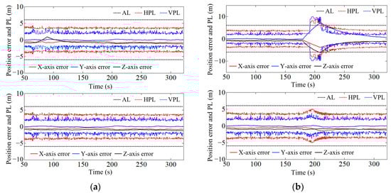
Figure 8.
Position error and protection-level curve. (a) Case 2; (b) Case 4.
Based on the positioning performance and protection level of the multi-source information fusion navigation system under fault-free conditions, the alarm limit for this experiment was tentatively set to 6 m (which needs to be set according to flight conditions in practice). When the alarm limit is exceeded, the system will issue an integrity alarm. It can be observed from Table 14 that for Case1 and Case2, the protection level without FI and with FI is essentially the same. Additionally, it can be seen from Figure 8 that the change in the protection level curve without FI and with FI is relatively small. This is because the positioning error caused by the fault itself is small, and the change mapped to the system protection level is also small.
From Figure 3b and Figure 8a, it is evident that the positioning error without FI actually decreases, causing the protection level not to change significantly. Thus, it is normal for the system not to generate integrity alarms. For Case4, Figure 8b illustrates that during the time period of the fault, the position error and protection level without FI significantly increased, quickly exceeding the set alarm limit, resulting in an integrity alarm. Table 14 corroborates this, showing that the protection level calculated in this paper surpasses the set alarm limit in both horizontal and vertical directions. Taking the vertical direction as an example, the VPLs of Case3 to Case5 exceed the alarm limit by 3.47 m, 6.12 m, and 4.15 m, respectively. Therefore, the system will generate integrity alarms, signifying that the current positioning information has lost its reliability. Additionally, Figure 4b indicates that the fault, when unisolated, will cause significant positioning errors. Considering the current alarm limit, the true position error has exceeded the alarm limit, and an integrity alarm should be issued. Figure 8 demonstrates that after the system correctly detects and isolates the fault navigation source, the system protection level calculated in this paper remains within the normal range during the fault time, and integrity alarms are not triggered.
6. Conclusions
In this paper, we propose a two-level integrity-monitoring method for multi-source information fusion navigation and report simulation tests conducted in an airborne environment. At the system level, the fault and verification model constructed by the loosely coupled Kalman filtered least-squares method can effectively detect and isolate faulty navigation sources. After passing the verification, the isolated sources can be re-incorporated into the fusion model. At the sensor level, suitable fault-detection models were constructed based on the redundancy of faulty navigation sources. Specifically, for the non-redundant navigation source TAN, different fault-detection methods were established according to its working mode to avoid mismatching. For the redundant navigation source GPS/BDS, the traditional method has been enhanced by optimizing the initial value of the fault-detection statistics using the expanded-dimension matrix. This optimization effectively reduces the detection delay caused by sub-filter adjustment. Finally, an integrity-risk dynamic allocation criterion was established to calculate the system-protection level for multi-source information fusion navigation. Simulation test results show that the method proposed in this paper can effectively detect, isolate, and verify faulty navigation sources and sensors. It issues integrity alarms in a timely manner without fault isolation, thereby improving the reliability of the navigation system.
Future works will focus on the following aspects: (1) in-depth investigation of integrity-monitoring methods under various fusion models; (2) further exploration of INS faults; (3) application of the proposed two-level integrity-monitoring structure in diverse scenarios. Additionally, the investigation of various fault-detection methods, such as machine learning, will be undertaken to enhance fault-detection performance.
Author Contributions
Methodology, software, and writing—original draft preparation, R.C.; writing—review and editing, L.Z. All authors have read and agreed to the published version of the manuscript.
Funding
This work was supported in part by the National Natural Science Foundation of China (Grant No. 42274037), the Aeronautical Science Foundation of China (Grant No. 2022Z022051001), the National Key Research and Development Program of China (Grant No. 2020YFB0505804).
Data Availability Statement
Data available on request due to restrictions eg privacy or ethical.
Conflicts of Interest
The authors declare no conflicts of interest.
References
- Sun, Y. Autonomous Integrity Monitoring for Relative Navigation of Multiple Unmanned Aerial Vehicles. Remote Sens. 2021, 13, 1483. [Google Scholar] [CrossRef]
- Wang, Z.; Li, B.; Dan, Z.; Wang, H.; Fang, K. 3D LiDAR Aided GNSS/INS Integration Fault Detection, Localization and Integrity Assessment in Urban Canyons. Remote Sens. 2022, 14, 4641. [Google Scholar] [CrossRef]
- Zhu, N.; Marais, J.; Bétaille, D. GNSS Position Integrity in Urban Environments: A Review of Literature. IEEE Trans. Intell. Transp. Syst. 2018, 19, 2762–2778. [Google Scholar] [CrossRef]
- An, H.; Yan, W.; Bian, S.; Ma, S. Rain Monitoring with Polarimetric GNSS Signals: Ground-Based Experimental Research. Remote Sens. 2019, 11, 2293. [Google Scholar] [CrossRef]
- Lee, Y.C.; Bian, B. Advanced RAIM performance sensitivity to deviation of ISM parameter values. In Proceedings of the 30th International Technical Meeting of The Satellite Division of the Institute of Navigation (ION GNSS+ 2017), Portland, OR, USA, 25–29 September 2017; pp. 2338–2358. [Google Scholar]
- Parkinson, B.W.; Axelrad, P. Autonomous GPS integrity monitoring using the pseudorange residual. Navigation 1988, 35, 255–274. [Google Scholar] [CrossRef]
- Diggelen, F.V.; Brown, A. Mathematical aspects of GPS RAIM. In Proceedings of the 1994 IEEE Position, Location and Navigation Symposium, Las Vegas, NV, USA, 11–15 April 1994; pp. 733–738. [Google Scholar]
- Madrid, P.F. Method for Computing an Error Bound of a Kalman Filter Based GNSS Position Solution; GMV Aerospace and Defense S.A.: Madrid, Spain, 2016. [Google Scholar]
- Feng, S.; Ochieng, W.; Moore, T. Carrier phase-based integrity monitoring for high-accuracy positioning. GPS Solut. 2009, 13, 13–22. [Google Scholar] [CrossRef]
- Blanch, J.; Walter, T.; Enge, P. Advanced RAIM user Algorithm Description: Integrity Support Message Processing, Fault Detection, Exclusion, Protection Level Calculation. In Proceedings of the 25th International Technical Meeting of the Satellite Division of the Institute of Navigation (ION GNSS), Nashville, TN, USA, 17–21 September 2012; pp. 2828–2849. [Google Scholar]
- Lee, Y.C. A position domain relative RAIM method. IEEE Trans. Aerosp. Electron. Syst. 2011, 47, 85–97. [Google Scholar] [CrossRef]
- Gioia, C.; Borio, D. Multi-constellation T-RAIM: An experimental evaluation. In Proceedings of the 30th International Technical Meeting of the Satellite Division of the Institute of Navigation, Portland, OR, USA, 25–29 September 2017; pp. 4248–4256. [Google Scholar]
- Vadlamani, A.; Haag, M. A 3D Spatial Integrity Monitor for Terrain Databases. In Proceedings of the 23rd Digital Avionics Systems Conference, Salt Lake City, UT, USA, 24–28 October 2004; pp. 796–809. [Google Scholar]
- Videmsek, A.; Haag, M. Terrain Referenced Integrity Monitor for An Unmanned Aircraft Systems Precision Approach. In Proceedings of the AIAA/IEEE 39th Digital Avionics Systems Conference (DASC), San Antonio, TX, USA, 11–15 October 2020; pp. 1–10. [Google Scholar]
- Vadlamani, A.; Haag, M. Improved Downward-Looking Terrain Database Integrity Monitor and Terrain Navigation. In Proceedings of the IEEE Aerospace Conference Proceedings, Big Sky, MT, USA, 6–13 March 2004; pp. 1594–1607. [Google Scholar]
- Pan, W.; Zhan, X.; Zhang, X. Fault exclusion method for ARAIM based on tight GNSS/INS integration to achieve CAT-I approach. IET Radar Sonar Navig. 2019, 13, 1909–1917. [Google Scholar] [CrossRef]
- Joerger, M.; Pervan, B. Kalman filter-based integrity monitoring against sensor faults. J. Guid. Control Dyn. 2013, 36, 349–361. [Google Scholar] [CrossRef]
- Hewitson, S.; Wang, J. Extended receiver autonomous integrity monitoring (eRAIM) for GNSS/INS integration. J. Surv. Eng. 2010, 136, 13–22. [Google Scholar] [CrossRef]
- Meng, Q.; Hsu, L.T. Integrity Monitoring for All-Source Navigation Enhanced by Kalman Filter based Solution Separation. IEEE Sens. 2021, 21, 15469–15484. [Google Scholar] [CrossRef]
- Cong, N. Research on Multi-Source Navigation Information Fusion and Fault Detection Algorithms; Harbin Engineering University: Harbin, China, 2021; pp. 89–92. [Google Scholar]
- Cui, Z.B.; Jing, B.; Jiao, X.X. Design of fault-tolerant integrated navigation system based on federated Kalman filter. J. Electron. Meas. Instrum. 2021, 35, 143–153. [Google Scholar]
- Zhang, Q.Q.; Zhao, L.; Zhou, J.H. A resilient adjustment method to weigh pseudorange observation in precise point positioning. Satell. Navig. 2022, 3, 16. [Google Scholar] [CrossRef]
- Jurado, J.D.; Raquet, J.F. Autonomous and Resilient Management of All-Source Sensors. In Proceedings of the ION 2019 Pacific PNT Meeting, Honolulu, HI, USA, 8–11 April 2019; pp. 142–159. [Google Scholar]
- Jurado, J.D.; Raquet, J.F.; Kabban, C. Residual-based multi-filter methodology for all source fault detection, exclusion, and performance monitoring. Navigation 2020, 67, 493–509. [Google Scholar] [CrossRef]
- Jurado, J.D.; Raquet, J.F.; Kabban, C. Single-Filter Finite Fault Detection and Exclusion Methodology for Real-Time Validation of Plug-and-Play Sensors. IEEE Trans. Aerosp. Electron. Syst. 2021, 57, 66–75. [Google Scholar] [CrossRef]
- Sepulveda, L.E. Optimizing a Bank of Kalman Filters for Navigation Integrity; Air Force Institute of Technology: Dayton, OH, USA, 2021; pp. 24–52. [Google Scholar]
- de Oliveira, F.A.C.; Torres, F.S.; García-Ortiz, A. Recent Advances in Sensor Integrity Monitoring Methods—A Review. IEEE Sens. J. 2022, 22, 10256–10279. [Google Scholar] [CrossRef]
- Groves, P.D. Principles of GNSS, Inertial, and Multi Sensor Integrated Navigation Systems; Artech House: London, UK, 2013; pp. 559–615. [Google Scholar]
- Sun, R.; Qiu, M.; Liu, F.; Wang, Z.; Ochieng, W.Y. A Dual w-Test Based Quality Control Algorithm for Integrated IMU/GNSS Navigation in Urban Areas. Remote Sens. 2022, 14, 2132. [Google Scholar] [CrossRef]
- Chen, R.; Zhang, Q.Q.; Zhao, L. Optimal Selection and Adaptability Analysis of Matching Area for Terrain Aided Navigation. IET Radar Sonar Navig. 2021, 15, 1702–1714. [Google Scholar] [CrossRef]
- Zhai, Y.; Zhan, X.; Pervan, B. Bounding Integrity Risk and False Alert Probability Over Exposure Time Intervals. IEEE Trans. Aerosp. Electron. Syst. 2020, 56, 1873–1885. [Google Scholar] [CrossRef]
- Jiang, H.T.; Li, T.; Song, D. An Effective Integrity Monitoring Scheme for GNSS/INS/Vision Integration Based on Error State EKF Model. IEEE Sens. J. 2022, 22, 7063–7072. [Google Scholar] [CrossRef]
- Chen, R.; Zhao, L. Multi-level autonomous integrity monitoring method for multi-source PNT resilient fusion navigation. Satell. Navig. 2023, 4, 21. [Google Scholar] [CrossRef]
- Blanch, J.; Walter, T. Fast Protection Levels for Fault Detection with an Application to Advanced RAIM. IEEE Trans. Aerosp. Electron. Syst. 2021, 57, 55–65. [Google Scholar] [CrossRef]
- Milner, C.; Pervan, B. Bounding Fault Probabilities for Advanced RAIM. IEEE Trans. Aerosp. Electron. Syst. 2020, 56, 2947–2958. [Google Scholar] [CrossRef]
Disclaimer/Publisher’s Note: The statements, opinions and data contained in all publications are solely those of the individual author(s) and contributor(s) and not of MDPI and/or the editor(s). MDPI and/or the editor(s) disclaim responsibility for any injury to people or property resulting from any ideas, methods, instructions or products referred to in the content. |
© 2023 by the authors. Licensee MDPI, Basel, Switzerland. This article is an open access article distributed under the terms and conditions of the Creative Commons Attribution (CC BY) license (https://creativecommons.org/licenses/by/4.0/).