Article

Multi-Level Attention Interactive Network for Cloud and Snow Detection Segmentation

1
Collaborative Innovation Center on Atmospheric Environment and Equipment Technology, Nanjing University of Information Science and Technology, Nanjing 210044, China
2
College of Information Science and Technology, Nanjing Forestry University, Nanjing 210037, China
3
Jiangsu Key Laboratory of Big Data Analysis Technology, Nanjing University of Information Science and Technology, Nanjing 210044, China
*
Author to whom correspondence should be addressed.
Remote Sens. 2024, 16(1), 112; https://doi.org/10.3390/rs16010112
Submission received: 31 October 2023 / Revised: 30 November 2023 / Accepted: 7 December 2023 / Published: 27 December 2023
(This article belongs to the Section Remote Sensing Image Processing)

Abstract

:
The ground is typically hidden by cloud and snow in satellite images, which have a similar visible spectrum and complex spatial distribution characteristics. The detection of cloud and snow is important for increasing image availability and studying climate change. To address the issues of the low classification accuracy and poor generalization effect by the traditional threshold method, as well as the problems of the misdetection of overlapping regions, rough segmentation results, and a loss of boundary details in existing algorithms, this paper designed a Multi-level Attention Interaction Network (MAINet). The MAINet uses a modified ResNet50 to extract features and introduces a Detail Feature Extraction module to extract multi-level information and reduce the loss of details. In the last down-sampling, the Deep Multi-head Information Enhancement module combines a CNN and a Transformer structure to make deep semantic features more distinct and reduce redundant information. Then, the Feature Interactive and Fusion Up-sampling module enhances the information extraction of deep and shallow information and, then, guides and aggregates each to make the learned semantic features more comprehensive, which can better recover remote sensing images and increase the prediction accuracy. The MAINet model we propose performed satisfactorily in handling cloud and snow detection and segmentation tasks in multiple scenarios. Experiments on related data sets also showed that the MAINet algorithm exhibited the best performance.

1. Introduction

Remote sensing satellites conduct long-term observations of the Earth, capturing and characterizing surface information [1,2]. Clouds cover more than half of the Earth’s surface [3], and nearly half of the Northern Hemisphere is covered by snow in winter [4]. Cloud and snow are present in many satellite images, blurring surface objects and reducing the utilization of the observed data [5]. However, in the study of climate–human–environment interactions [6], they play a crucial role in researching climate change, investigating hydrological resources, and issuing snow disaster warnings [7]. Due to the close radiation temperatures and similar properties in the optical wavelengths of snow and clouds, distinguishing between the two during detection tasks is challenging [8].
Researchers have carried out a variety of recognition studies for different satellite image data. Traditional methods primarily detect clouds or both clouds and snow by analyzing variations in the electromagnetic wave reflection or radiation properties between targets [9]. Gladkova et al. [10] proposed an enhanced method for cloud and snow identification and briefly analyzed the classification problem with clouds and snow. Ding et al. [11] proposed an automated discrimination approach for cloud and snow in full-color images using fractal dimensions. Zhu et al. [12] improved the Fmask algorithm using a threshold-detection method based on multispectral bands. After testing the data collected from Landsat8, it was found that the wavelength information in the data could be effectively utilized to identify cloud bands. Wang et al. [13] also used the normalized difference index to extract the features of snow regions in satellite images to realize the identification of each region. The threshold methods used in the above methods all require professionals to perform threshold calibration in advance, and these methods basically extract single features of clouds and snow. Additionally, some machine learning algorithms use trained classifiers to detect clouds and snow [14,15,16,17]. Sun et al. [18] suggested a recognition approach based on various texture features of images, using an SVM classifier with an RBF kernel for detection after extracting texture features. Ghasemian et al. [19] fused multiple features for detection based on two random forest algorithms. Kang et al. [20] suggested a coarse-to-fine approach that extracted the statistical features and performed an SVM operation on the superposition features to produce the initial cloud-detection map, then honed the limits using guided filtering. Detection accuracy can be improved as greater-level features including texture, shape, and contours are used in these methods. However, due to limitations in trainable parameter capacity, some machine learning techniques have proven inferior to Fmask in complex tasks [21].
Deep learning, as a subfield of machine learning, has achieved significant advances in image processing [22,23,24]. The fact that all characteristics are automatically learned from enormous data sets distinguishes deep learning from conventional algorithms the most. Artificial feature extraction relies on experts and is unable to effectively utilize the benefits of large data, while deep learning can swiftly learn efficient representations to extract features from images, improving accuracy, reasoning speed, and generalization ability [25]. Meanwhile, CNNs have been used in numerous detection studies with successful results [26,27]. Zhan et al. [28] suggested the method based on the FCN framework [29] employing satellite images in three visible wavelengths for recognition. Xie et al. [30] proposed a method that combines clustering and a CNN. First, superpixels are obtained by improving SLIC clustering, and then, the CNN extracts features from the superpixels, which can obtain relatively accurate cloud boundary information, but cannot achieve end-to-end cloud detection. Chai et al. [21] proposed SegNet for detection in Landsat images with an encoder–decoder structure, but the problem of misjudgment caused by the lack of understanding of global semantic information exists. Zhang et al. [31] proposed CSD-Net with multi-scale feature fusion for the detection inpictures from different sensors.
There are currently many types of remote sensing images, among which the increasing number of medium- and high-spatial resolution images at the visible and near-infrared wavelengths has greatly promoted research in the field of snow and cloud discrimination. Although there are many ways to achieve this task, the detection results still have certain shortcomings. First of all, due to the limited feature extraction capabilities, traditional methods cannot automatically extract the high-order semantic features of cloud and snow areas and ignore some valuable features, resulting in poor generalization capabilities and robustness. Secondly, existing deep learning methods cannot detect the tiny areas covered by powder snow and thin clouds in some scenes well, resulting in overlapping objects and the incorrect detection of junctions. Therefore, it is necessary to improve boundary detail prediction and small-scale object recognition. Finally, the development of satellite images towards high resolution increases the demand for high-resolution image detection and requires the application of enhanced methods to high-resolution images.
Our research leveraged deep learning techniques to develop a powerful algorithm specifically designed to differentiate between snow and clouds in medium- and high-resolution visible light remote sensing images. As a novel method, this model solves the above-mentioned problems to a certain extent, helps to improve image analysis capabilities in rapidly growing data sets, and increases the development prospects of visible spectrum image classification. This research proposes an encoder–decoder network structure approach based on ResNet [32] to overcome the issues while boosting the accuracy and reliability of cloud and snow categorization, which is suitable for medium- and high-resolution pictures in the visible light wavelengths and was tested on the CSWV dataset. This model improved the network structure in the feature fusion stage, introduced channel spatial attention, added a Transformer module and other operations to strengthen the detection of edges and small areas of thin cloud and fine snow, and added an auxiliary loss function and other methods to accelerate the training convergence.
The test results demonstrated that MAINet outperformed the current CNN model, effectively fulfilling the cloud and snow segmentation task and enhancing recognition accuracy. Furthermore, our model exhibits significant applicability and universality. Compared with previous detection methods, it can better use image features for segmentation and can be applied to multiple types of images. In summary, the following are the primary contributions of the proposed approach:
  • A new cloud and snow detection network, a Multi-level Attention Interactive Network (MAINet), is proposed to strengthen the attention to the details of cloud and snow, which only uses visible channel remote sensing images to achieve higher detection accuracy and faster detection speed.
  • Detail Feature Extraction (DFE) is supplied to extract the sameness and difference between the information in the down-sampling stage, reduce the information loss, strengthen the detail information, and realize the refinement of the edge;
  • Deep Multi-head Information Enhancement (DMIE) is created in the last step of down-sampling. The CNN and Transformer structures were combined by bridging units to accomplish the purpose of retaining local and global features, which can more deeply mine the relationship between deep features and enhance the network’s capacity for representation;
  • Feature Interaction and Fusion Up-sampling modules (FIFU) is also proposed in the up-sampling process to restore remote sensing images more effectively and improve prediction accuracy, which consists of three small blocks. The MSBC block extracts multi-scale information and captures edge feature. The SCA block uses a spatial and channel feature attention mechanism to enhance the spatial relationship information and important channel information. The SFIF block aggregates the two types of information and guides them to make the semantic features of the cloud and snow more complete and boost the effectiveness of feature extraction.

2. Methodology

Because of the similarities between cloud and snow, as well as the spatial distribution characteristics being complex and changeable, many traditional networks cannot achieve the accuracy of segmentation and have various issues including false detections of cloud and snow overlap area and rough segmentation boundaries. Meanwhile, the improvement of image resolution brings more-precise information and localization information. This paper introduces MAINet to accurately segment clouds and snow. MAINet strengthens the extraction ability, enhances the recovery of details, and effectively uses context information for information aggregation optimization, so as to achieve more-accurate predictions.
In this part, the MAINet architecture proposed is firstly introduced, which uses ResNet as the backbone for cloud and snow segmentation, and then, focuses on three modules: DFE, DMIE, and FIFU.

2.1. Network Architecture

The overall structure of MAINet is represented in Figure 1. We adopted an encoder–decoder structure and used ResNet50 [32] as the backbone, which solves the issue of traditional methods struggling to automatically extract high-order semantic information from cloud and snow regions in images. The reason for selecting ResNet lied in the concept of residual learning, which, to some extent, solves issues such as gradient disappearance, explosion, and degradation. This reduces the difficulty of network learning. Additionally, each layer of the network contains various degrees of semantic characteristics, facilitating the rapid extraction of multi-scale data. It is beneficial to retain more original semantic information. However, the computational load for the segmentation task is substantial. Lin et al. [33] demonstrated that a 1 × 1 convolution may alter the number of channels, reducing or increasing the dimension of the information. Therefore, a 1 × 1 convolution was employed at decoder stage to reduce the overall parameters of MAINet.
Due to the difficult of extracting the complex features of cloud and snow in the visible spectrum, we propose the DMIE module as the deepest part of the backbone network to improve the representation capacity. Its function is to use the Transformer [34] concept at the end of the down-sampling to enhance the global perception ability on the channel, extract accurate dense features, and combine local features with global features, which can weaken or remove interference information and deeply mine high-order semantic information. Secondly, due to the issues with inaccurate segmentation results and the loss of boundary details in the current algorithm, the DFE module is proposed to establish skip connections between the features of the encoder and decoder, which can transmit the low-level information to the network’s deep layers. This operation can enhance high-frequency spatial feature information and achieve edge refinement while recovering lost details in the encoder stage. Finally, due to the simple merging operation of high-level and low-level features, the lost details cannot be effectively recovered, and the false detection in the overlapping area and the misdetection of tiny regions cannot be alleviated. We propose the FIFU module to address this issue. FIFU enhances the feature information extraction at different levels through the attention mechanism, aggregates the information between different scales, connects them with each other, and fuses the element representations, which provides more-effective features for the up-sampling process. This operation can reduce false detection in the overlapping area, strengthen detail detection of small areas, and improve prediction accuracy.
In addition, in the training phase of the MAINet model, as shown in Figure 2, we introduce two Auxiliary branches (AUX). These branches are included as the additional prediction outputs in the computation of the loss function. The purpose of the AUX is to increase prediction accuracy while speeding up the training processes. The first is a 3 × 3 convolutional layer with a Batch Normalization (BN) layer [35] and a Rectified Linear Unit (ReLU) activation layer. Then, unnecessary information is removed through the dropout layer. Finally, the prediction information is output through the 1 × 1 convolutional layer and enlarged to the original size through the up-sampling layer.

2.2. Deep Multi-Headed Information Enhancement

In visual descriptors, crucial correspondences exist between local characteristics and global representations [36]. Compact vectors called local features represent local image neighborhoods, while global representations encompass aspects such as contour representations, shape descriptors, long-distance object types, and more. Most CNN models excel at gathering local characteristics, but struggle to identify global features. Identifying characteristics in the segmented objects in space and spectrum is difficult in the cloud- and snow-segmentation tasks, requiring the effective extraction of deep global features across channels. In Visual Transformer (ViT) [37], the feasibility of the pure Transformer architecture in computer vision tasks was verified. ViT aggregates and compresses the global representation in patches in a soft way through the self-attention module, and the Transformer block is used as an independent architecture or introduced into the CNNs [38,39,40].
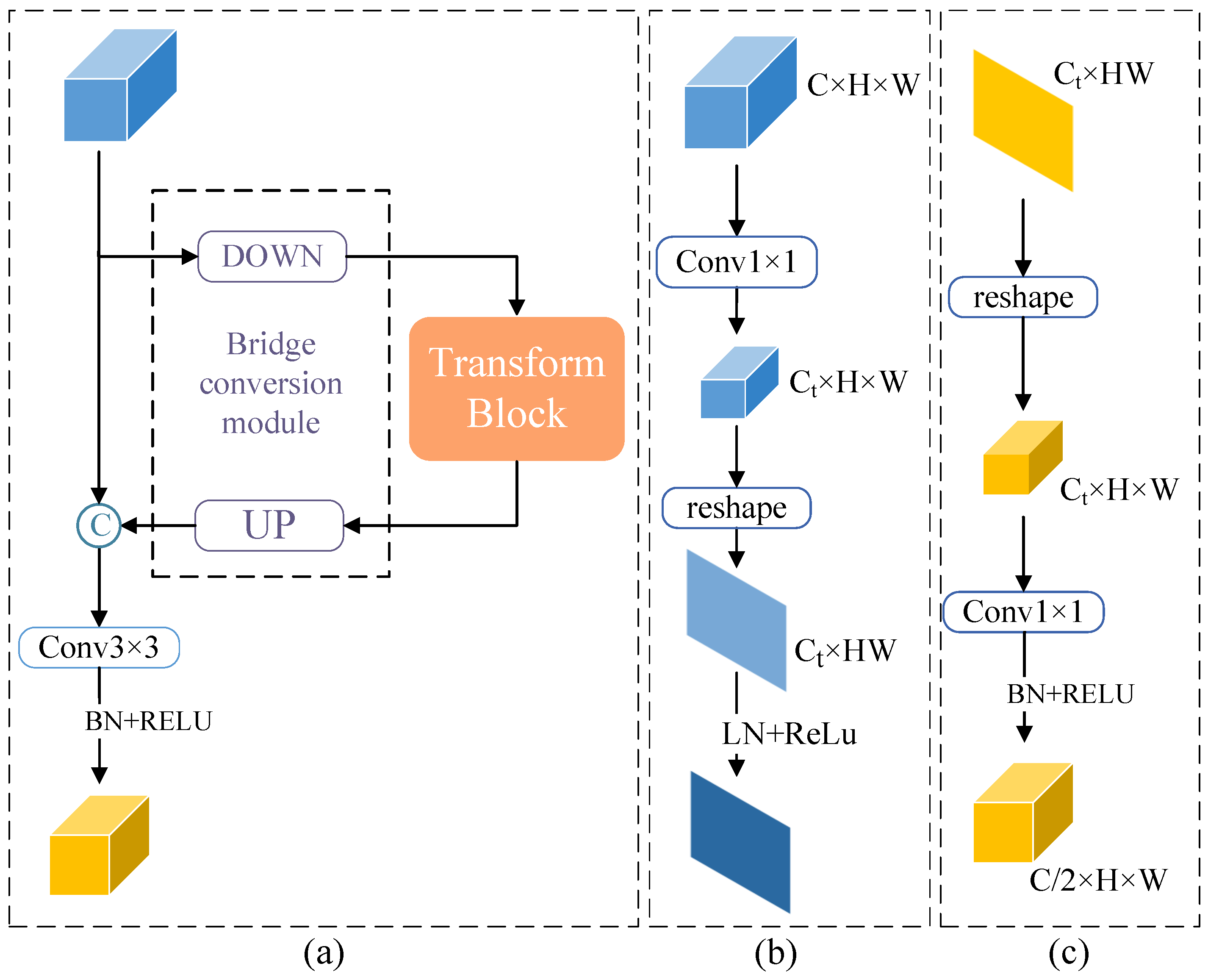
We designed the DMIE module shown in Figure 3 by drawing inspiration from ViT and used the Transformer attention mechanism to promote global perception across channels. This module can shuffle channels, gathers context information by filtering redundant data, properly extracts deep global features, and outputs them after interacting with the input fusion. However, if the input information is not properly fused with the Transformer, the quality of local details may suffer. Therefore, the Bridge-Conversion Module (BCM) is used to fuse local details from the CNN and global perceptionfrom the Transformer. This process involves the interaction of the two for a better feature-extraction result.
The final output of the backbone is fed into DMIE. Since the Transformer and CNN have different feature sizes, we needed fuse the feature in the CNN with the patch embeddings in the Transformer. Therefore, we used the BCM to accomplish the interactive coupling of the local and global features. The first step is to pass through the BCM_DOWN part in Figure 3b. The number of input channels C was compressed into the Transformer using the number of channels C t of the Transformer using patch embeddings through a 1 × 1 convolution. Then, the CNN feature from B × C t × H × W is converted to the shape of the patch embeddings in Transformer B × HW × C t , and the LayerNorm [41] is used to normalize the features. After ReLU activation, the feature enters the Transformer block, as illustrated in Figure 4.
The Multi-head self-attention block provides multiple representation subspaces for the attention layer of the model. Three independent, randomly initialized weight matrices are utilized. Then, the vectors are translated into different subspaces, enriching the feature expression and enabling the model to focus on multiple key regions. To reduce the effects of drastic changes in the model parameters during training and make the network learn more stably, the LayerNorm is applied before the Multi-head self-attention block and MLP block.
Next, the feature received from the Transformer is input into the BCM_UP to restore the form of the patch embeddings in the Transformer from B × HW × C t to the form of the CNN feature map B × C t × H × W, and passes a 1 × 1 convolution with BN and ReLU to convert the channel dimension to be mapped to C/2, as shown in Figure 3c. Finally, the CNN feature information and the Transformer feature information outputs are concatenated by the backbone network. A 3 × 3 convolution is used to encode and fuse the local and global features, obtaining the enhanced feature.
The DMIE module realizes the combination of the CNN and Transformer in the deep layer by the BCM. This means that the module can naturally inherit the advantages of the CNN and Transformer structure and retain the extraction ability of the local and global features to the greatest extent, which significantly improves the network’s ability to represent the features.

2.3. Detail Feature Extraction

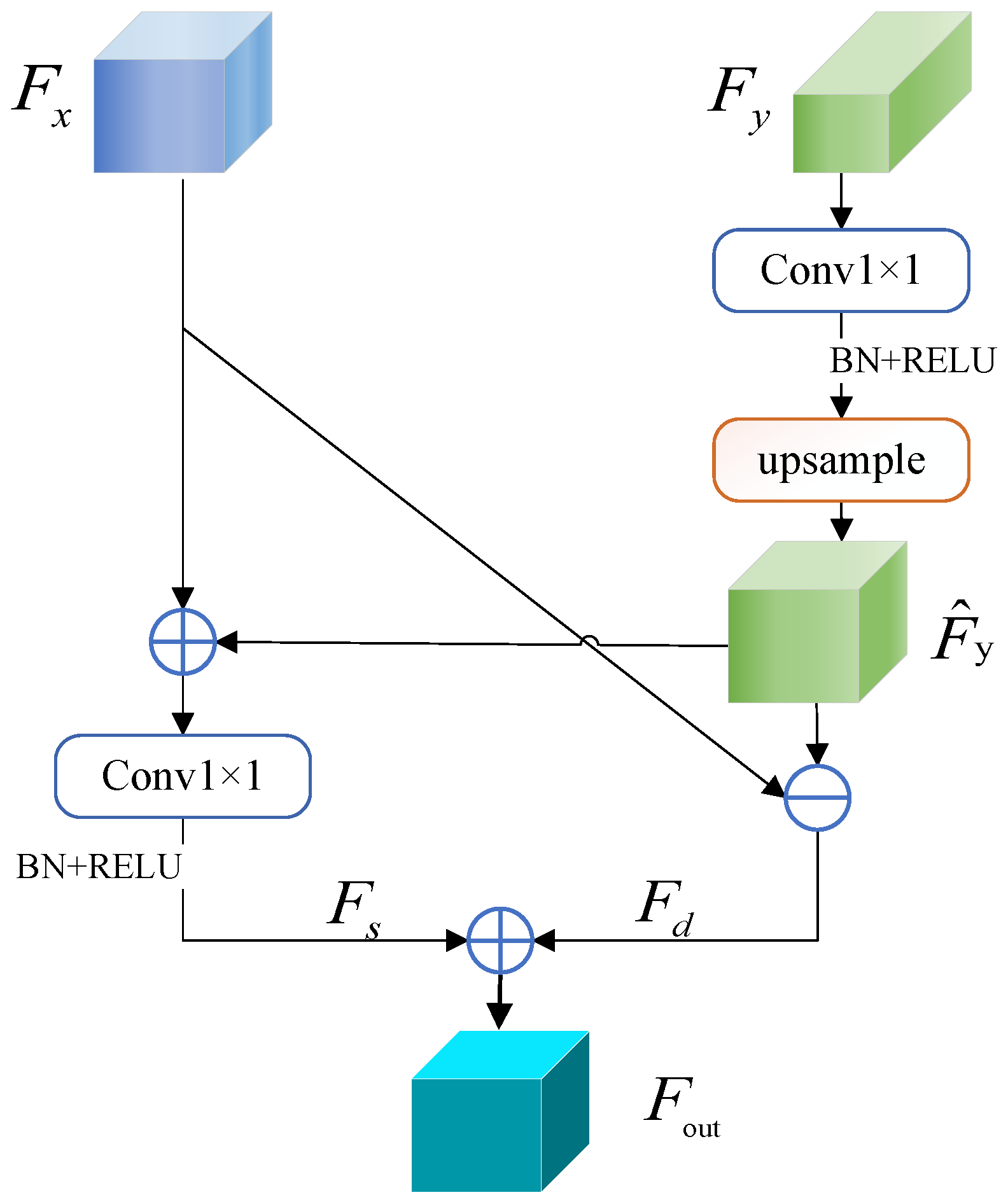
In the encoding process, the semantic branches of the classical network UNet [42] come from each layer, and it is merged from the same layers of the encoder and decoder by a layer hopping and splicing operation to combine the shallow geographical information with the deep semantics, which makes the network obtain good results. Meanwhile, considering that the basic model of deep learning usually adopts the down-sampling operation to reduce the information dimension, some details are inevitably lost [43]. To address this loss of information, we designed DFE as the intermediate bridging information, and its structure is shown in Figure 5.
Its input comes from two parts, F x from the shallow layer of the backbone and F y from the deep layer of the backbone. We initially performed convolution and up-sampling operations to make the deep feature map the same size as the shallow feature map before combining the shallow layer with the deep layer. Then, the difference detail information branch is obtained by subtracting the two parts, with a learnable parameter set to enable the network to independently adjust and focus on the important difference areas. Meanwhile, the two parts are added and extract the information by convolution to obtain the same information branch. Finally, we added the two branches to output the superposition of the features. The expression formula of the above steps is:
F ^ y = u p ( f B R 1 × 1 ( F y ) ) , F y R c / 2 × h / 2 × w / 2 , F ^ y R c × h × w
F d = λ × F x F ^ y , F x R c × h × w , F d R c × h × w
F s = f B R 1 × 1 ( F x + F ^ y ) , F s R c × h × w
F o u t = F s + F d ,
where F x is the shallow input; F y is the deep input; f B R 1 × 1 () is a 1 × 1 convolution with BN and ReLU. u p ( ) represents the up-sampling operation. F ^ y represents the deep input after up-sampling. F d represents the difference detail feature obtained by subtracting F x and F ^ y and multiplied by weight λ . F s represents the same detailed feature gained by adding F x and F ^ y . F o u t is the final detailed feature after stacking.
Through this design, we output the features at two scales, achieving a good compromise between location information and semantic information. The shallow feature and location information are propagated to the deep layer, which makes up for the details missed in the recovery stage of the encoder. This is extremely important for the recovery of image positioning.

2.4. Feature Interaction and Fusion Up-Sampling

In the feature fusion stage, this paper designed an up-sampling module based on the encoder–decoder segmentation network. The up-sampling process is crucial for forming clear high-resolution images. Using a simple basic decoder to directly fuse information will lead to semantic dilution, resulting in information redundancy, which affects the segmentation effect of the network. Therefore, we designed a FIFU module, shown in Figure 6, to complete the up-sampling feature fusion and restoration. This module mainly has two inputs: one is the high-resolution shallow feature generated by the branches of the shallow adjacent backbone layer through DFE, and the other is the low-resolution deep feature generated by the output of the last FIFU module or MIDE module. The model can rapidly and efficiently gather input due to this module. It pays attention to both the shallow features with spatial information and the deep features with context information. Features from different levels are fused to enhance the prediction precision, thereby improving the segmentation performance of MAINet.
The module is mainly divided into two stages and comprises three parts: Multi-scale and Strip Boundary Convolution (MSBC) block, Spatial Channel Attention (SCA) block and Spatial Feature Interactive Fusion (SFIF) block, and is mainly separated into two stages. The first stage is mainly to enhance the interaction process of the two pieces of input feature information. In this stage, the MSBC block interaction is used for shallow feature map input, and various scales of convolutional kernels are used to obtain multi-scale receptive fields, while strip convolution is used to enhance boundary detection. The SCA block is used for deep features to enhance the spatial and channel attention for the deep information. In the second stage, the two branches interact with the semantic information before entering the SFIF block, and then, new features are generated by using addition between high-level and low-level features to guide each other. This approach allows high-resolution and low-resolution representations in each layer to repeatedly receive information, reducing semantic information loss and obtaining abundant features. Finally, the SFIF block is used to combine the new features obtained after enhancing the two features.

2.4.1. Multi-Scale and Strip Boundary Convolution

While the shallow feature map extracts high-frequency detail information through DFE, the noise of the shallow feature will also be introduced, so we intended to further filter the data using the convolution layer. We designed MSBC to filter the shallow feature map, further extracting multi-scale features and enhancing segmentation boundary features.
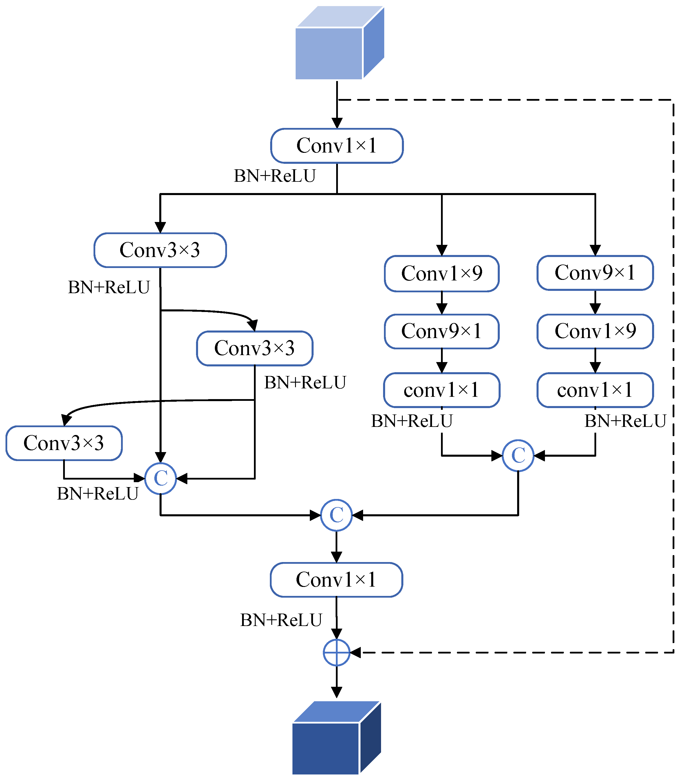
The MSBC shown in Figure 7 consists of a 1 × 1, 3 × 3 convolution and strip convolution. Each convolution, except the strip convolution, is followed by BN and ReLU. The input low-level feature initially undergoes a 1 × 1 convolution to compress the channels to half of their initial count. This operation can reduce the network parameters to prevent memory overflow. Afterwards, the boundary feature information is extracted from the right branch, while the multi-scale feature is fused and extracted from the left branch.
For the left branch, since expressing features at various sizes is crucial for many vision applications, we enabled the block to aggregate the receptive fields of 3 × 3, 5 × 5, and 7 × 7 by combining different numbers of 3 × 3 convolutional structures. In addition, all of the 3 × 3 convolutions perform grouped convolution operations, which further reduces the amount of network parameters. The feature data from various receptive field sizes are concatenated together to form a convolution combination, the combination of which helps to tackle the object detection at different scales and represents features more specifically.
For the right branch, since cloud and snow can vary in size and shape and be closely connected to each other, the boundary between cloud and snow is difficult to determine, and the segmentation boundary is rough and lacks detail. To address this problem, we employed strip convolution to forecast the border and decrease interference in unrelated areas. Specifically, a 9 × 9 convolution was designed as a parallel cascade by using the splitting method. The two branches are the convolution operation, which consists of 9 × 1 and 1 × 9. After that, the channel information of both branches is compressed by a 1 × 1 convolution, and the channel number is halved again to concat the two branches together. The horizontal strip convolution learns the horizontal features, and the vertical strip convolution has similar effects, which effectively capture the edge feature, where cloud and snow converge.
Finally, we concatenated each branch along the channel, then passed through a 1 × 1 convolution to compress the channels to the original number and used a residual structure to introduce a skip connection represented by the rightmost black dotted line. The desired feature is formed by adding the initial input to the output of the aforementioned process.

2.4.2. Spatial Channel Attention

The receptive field of the convolutional kernel is local [44], which is only associated with different separate parts in the image after multi-layer accumulation, and the pixels in the center of the receptive field have a greater impact on the output. It is important to focus on the pixels that have a significant influence on a pixel’s local feature aggregation, so we propose the SCA block, as shown in Figure 8. This block connects the cloud and snow with the surrounding feature information and enhances the spatial channel attention information to better distinguish the difference between ground objects.
The input F R c × h × w is the deep feature information branch shown in Figure 8b. First, the SpatialAttention block can capture long-range dependency information and solve the problem of local receptive fields. F is passed through three 1 × 1 convolutional blocks, which produce three feature maps F 1 R c × h × w , F 2 R c × h × w , and F 3 R c × h × w ( c is c / 8 ). Afterwards, F 1 is reconstructed as F ^ 1 R h × w × c , and F 2 is reconstructed in the same way and, then, transposed to obtain F ^ 2 R c × h × w . The spatial attention S R h × w × h × w is created by multiplying the two maps ( F ^ 1 , F ^ 2 ) together and, then, applying a softmax to the resulting matrix. Finally, the third branch feature is reshaped as F ^ 3 R c × h × w like the other branches. The output F S R c × h × w is generated after F S is multiplied by S, and the calculation result is reconstructed to the original scale. The following is the calculating formula:
F ^ 1 = θ ( f 1 × 1 ( F 1 ) ) , F ^ 2 = φ ( f 1 × 1 ( F 2 ) ) , F ^ 3 = g ( f 1 × 1 ( F 3 ) ) ,
S = σ F ^ 1 F ^ 2 ,
F S = S F ^ 3 ,
where f 1 × 1 represents a 1 × 1 convolution; θ (), φ (), g() represent different reconstruction methods; ⨂ represents matrix multiplication; σ () is the softmax operator.
The ChannelAttention block shown in Figure 8c can capture the dependencies existing between channels and enhance the specific semantic feature representation. We compressed the input features by two methods: average pooling and max pooling, and aggregated the features obtained from the two compressions. The feature maps F add R c × 1 × 1 and F cat R 2 c × 1 × 1 are obtained by the add and concat operation, respectively. They are input into a two-layer fully connected layer (MLP). The number of neurons in the first layer is C/r; r was set to 16 considering efficiency. The shared second MLP layer was set to C number of neurons. After that, the output is summed and activated by the sigmoid function to provide the channel attention features. The calculation formula is as follows:
F avg = A v g P o o l F , F max = M a x P o o l F ,
F add = F avg + F max , F cat = ( F avg , F max ) ,
F c = δ W 2 W 0 F add + W 2 W 1 F cat ,
where W 0 and W 1 , respectively, represent the weights of F add and F cat in the first MLP layer; W 2 represents the shared weight of F add and F cat in the second MLP layer. δ () is the sigmoid function, and F c represents the channel attention feature.
Finally, CSA multiplies the input features with the spatial attention features and channel attention features and performs an elementwise sum operation to generate the final output synthetic attention features, which is described as follows:
F s c = f 1 × 1 F F s + F F c ,
F o u t = δ B N ( F s c F ) ,
where ⨂ represents matrix multiplication, F s c represents the features obtained by combining the spatial attention features and channel attention features, BN is Batch Normalization, δ ( · ) is the ReLU activation, and F o u t is the final output of the block.
The CSAM block increases the spatial channel information of the deep features by merging two feature attention techniques, allowing the model to concentrate on the crucial information over the entire image while suppressing or even ignoring certain unimportant noise information.

2.4.3. Spatial Feature Interactive Fusion

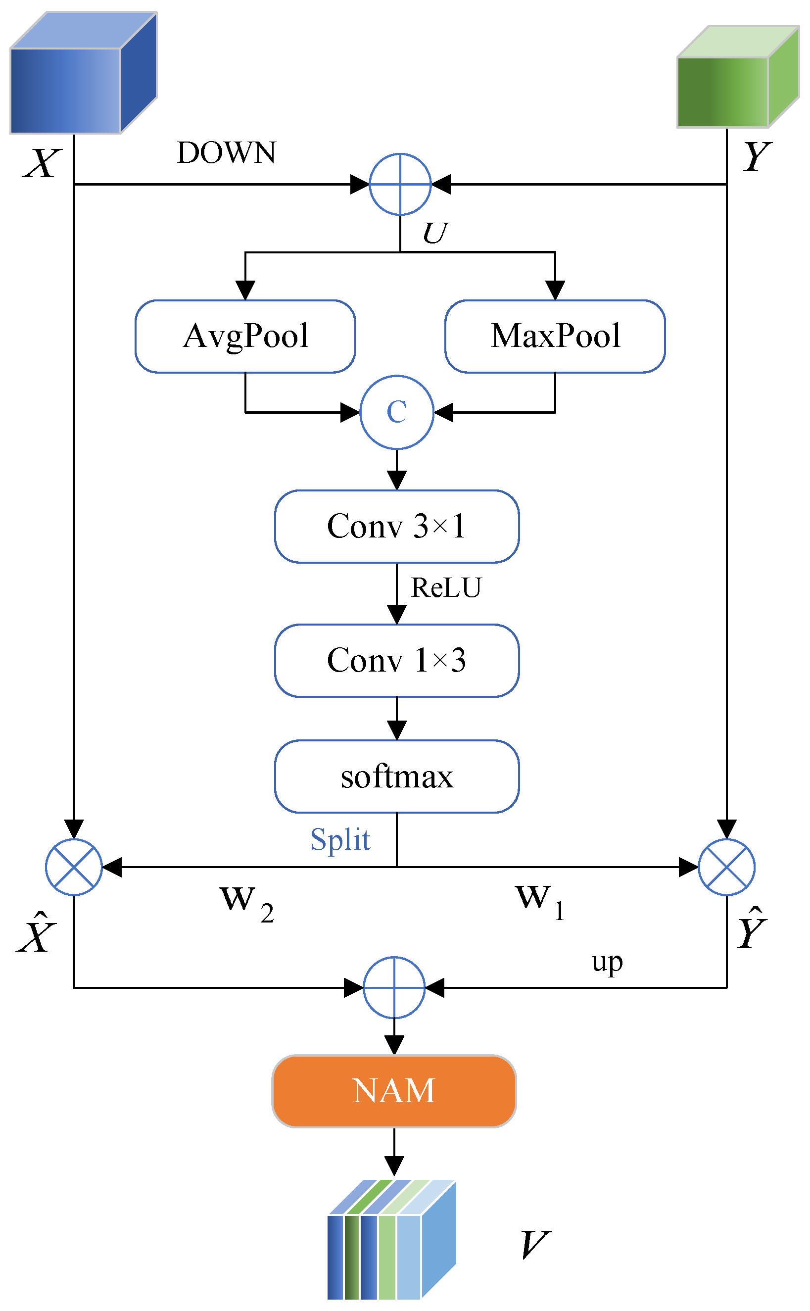
The shallow and deep feature branches each possess distinct advantages in terms of their characteristics. These two branches interact with the semantic information through addition before fusion, resulting in rich feature representations. To better aggregate the features of two branches into a multi-level/multi-scale feature map, we designed SFIF to make both branches able to mentor one another during learning. In the feature-fusion step, this block employs a parallel spatial attention mechanism, allowing the model to swiftly gather pertinent information and increase prediction precision. In addition, we added the NAM attention module proposed by Liu et al. [45] to suppress less-significant features.
Figure 9 depicts SFIF’s structural layout. We cross-mapped the features of the two input branches to produce the spatial attention weights. First, the shallow map X R c × h × w is mapped to the size R c / 2 × h / 2 × w / 2 by down-sampling and added to the deep feature Y R c / 2 × h / 2 × w / 2 to form the input of the spatial attention U R c × h / 2 × w / 2 . The max-pooling and average-pooling processes are employed to produce the spatial attention, and the spatial information is extracted through two layers of convolution, then a softmax operation is run to obtain the weights for the spatial attention. The following formula is the final spatial attention weight w R 2 × h × w :
U = Y + d o w n X ,
w = f 1 × 3 ( f 3 × 1 ( F c a p U ; F c m p ( U ) ) ) ,
w 1 ; w 2 = σ w ,
where d o w n ( · ) is the down-sampling operation; F c a p ( ) and F c m p ( ) are the average-pooling and max-pooling; f 1 × 3 () and f 3 × 1 () are 1 × 3 and 3 × 1 convolution operations; σ ( ) is the softmax operator.
High-resolution features Y ^ R h × w × c ; low-resolution features X ^ R c × h / 2 × w / 2 ; the final fused features V R c × h × w . We split w into two parts, w 1 R c × h × w and w 2 R c × h × w , to express the space weight of Y and X; the process can be computed as follows:
Y ^ = w 1 Y ,
X ^ = w 2 X ,
V = N A M u p Y ^ + X ^ ,
where ⨂ is matrix multiplication and u p ( ) is up-sampling using bilinear interpolation. The added fused feature information is then passed through the NAM block, and the weight of less-significant features is reduced by applying a sparse weight penalty. Lastly, we obtained V, which was optimized by the spatial attention. The SFIF module uses less computation and parameters to strengthen the effective spatial information and effectively fuses the information of different branches, making the prediction result clearer.

3. Experiment

3.1. Dataset Introduction

In this experiment, the images of the CSWV and HRC_WHU datasets used were cropped to 256 × 256 px, and the images with only one class were deleted. The sorted patches were randomly split into a 0.8:0.2 training set and validation set, and the deep convolutional neural network learning optimization, unbiased evaluation, and final evaluation were carried out, respectively.
Overfitting happened during training due the small quantity of training data. To increase the amount of picture patches and accompanying labels, we used data augmentation, which enhanced the robustness of the network without increasing the amount of manual labels [29]. Transformation enhancement techniques combining color, contrast, and geometric elements were abandoned in favor of a random rotation inversion operation because of the minor spectral variations and intricate natural forms of snow and clouds.

3.1.1. CSWV Dataset

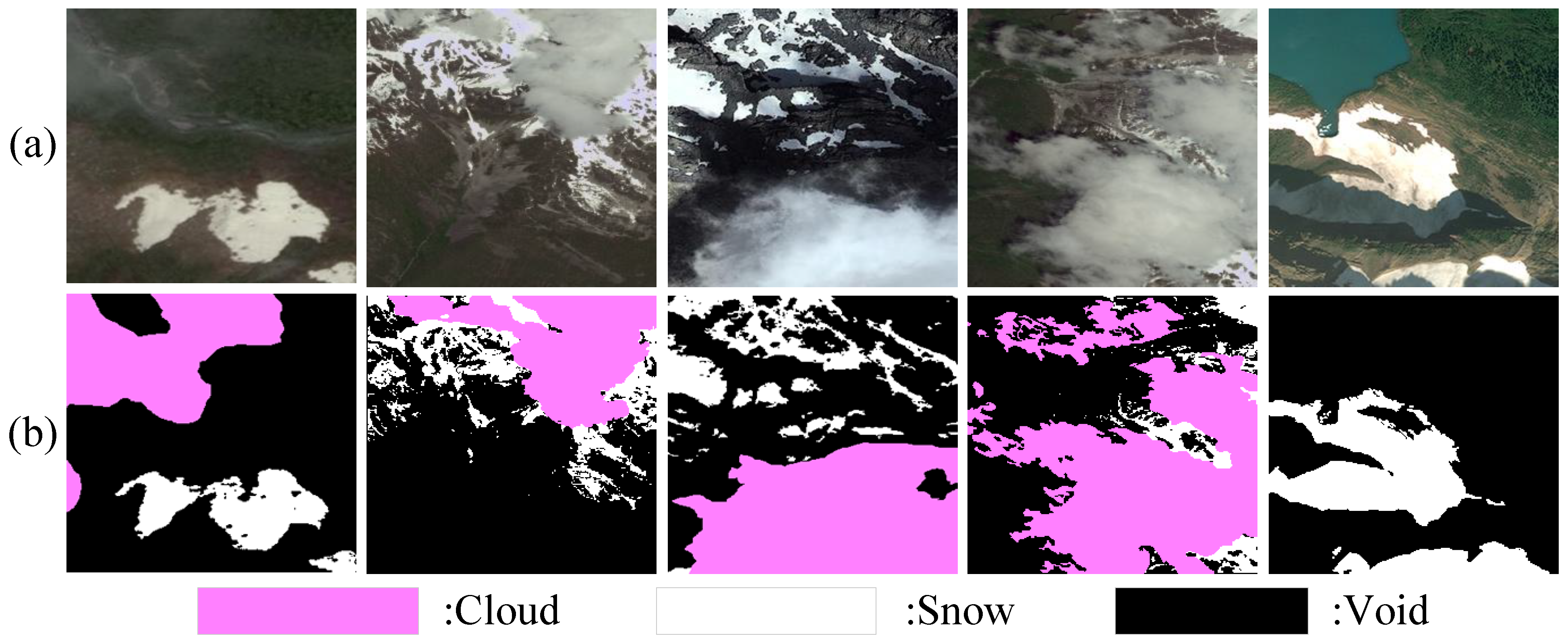
The major task was to use high-resolution images for cloud and snow detection. This paper used the public CSWV dataset [31], as shown in Figure 10, which was constructed based on WorldView2, and the spatial resolution is 0.5–10 m. It contains 27 cloud and snow images from WorldView2 in the Cordillera Mountains of North America, taken between June 2014 and July 2016. These scenes have a complex surface, including forests, grasslands, lakes, bare ground, and so on, resulting in a total of 9594 images. There is a variety of clouds including cirrus, cirrocumulus, altocumulus, cumulus, and stratus.

3.1.2. HRC_WHU Dataset

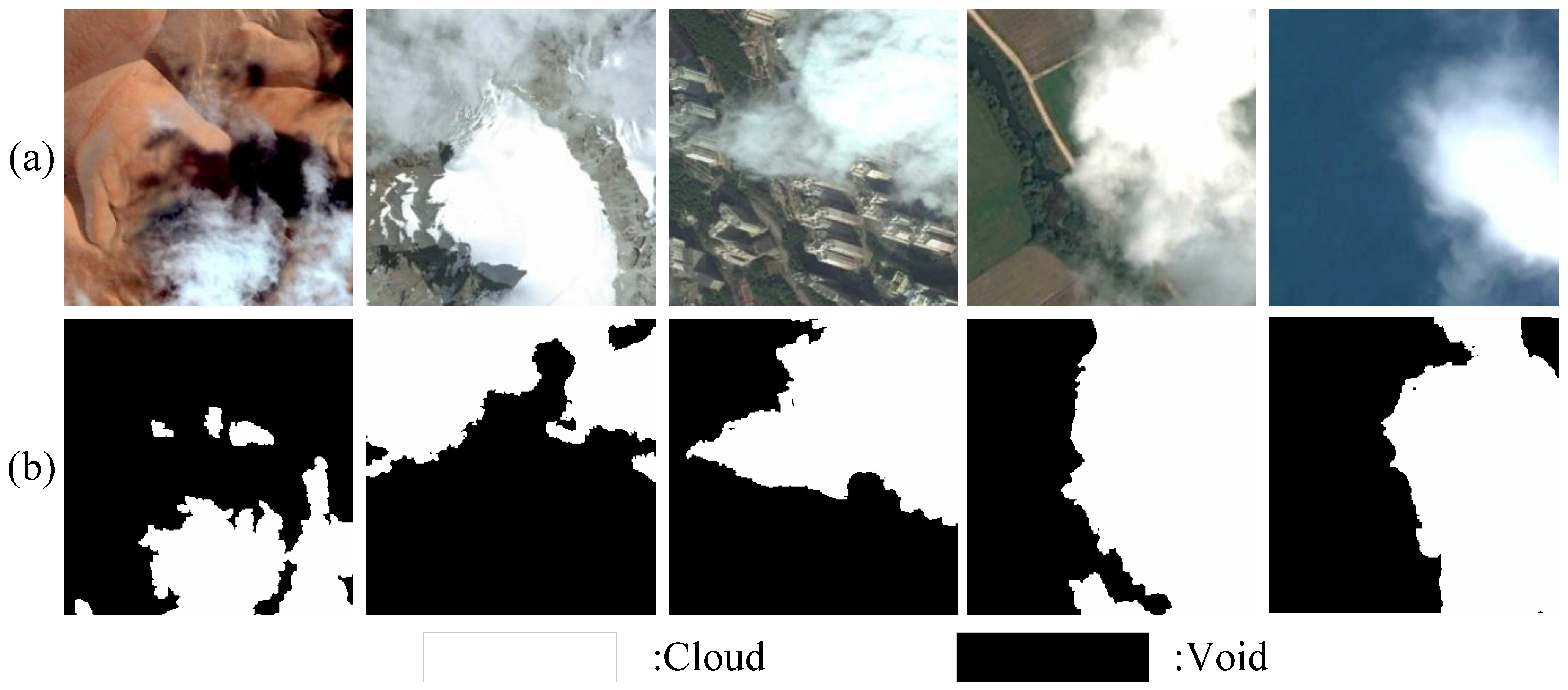
We assessed the generalization ability of related models using the public HRC_WHU dataset produced by Li et al. [46]. There are five main types of land cover represented in this dataset from Google Earth: water, vegetation, urban, snow/ice, and barren. The pertinent reference cloud masks were digitized by Wuhan University specialists in the field of remote sensing image interpretation. A total of 5996 high-definition images were generated in this dataset after data augmentation, and the number of channels was 3, as shown in Figure 11.

3.2. Experimental Setup

The deep learning framework of Python 3.8, PyTorch 1.10.1, and CUDA 11.1 served as the foundation for all model experiments. The training and testing procedures were carried out on a Windows 10 64 bit computer with an Intel Core i7-11700F @ 2.50 GHz CPU and NVIDIA RTX3080 installed.
We chose the Adaptive Moment Estimation (Adam) optimizer [47] as the gradient descent in the training. The Adam optimization is a stochastic gradient descent extension that uses second-order moment estimation to adaptively adjust the learning rate. Since the learning rate is an essential element of the deep learning training process, we employed the poly learning rate approach to dynamically change it [48]. This is the calculation formula:
l u = l i × 1 e p o c h m a x _ e p o c h p
where l u is the updated learning rate, l i is the initial learning rate, e p o c h is the current iteration, m a x _ e p o c h is the maximum number of iterations, and p is a constant that controls the rate of decay. We set l i to 0.00015, m a x _ e p o c h to 250, p to 0.9, the batch size to 8, and also, chose the classification cross-entropy function as the loss function.
This paper set the auxiliary loss and main loss jointly to monitor the learning during the training, which drew inspiration from Zhao et al. [49]. Auxiliary loss is introduced into a deep network to aid in learning optimization without impacting the learning of the main branch. We offered three levels of semantic headers, including the primary loss, to make the parameter adjustment easier. The loss function formula is as follows:
L Θ = λ 1 L m Θ + λ 2 L a 1 Θ + λ 3 L a 2 Θ ,
where L m is the main loss and L a 1 and L a 2 are the auxiliary loss of branch 1 and branch 2. The loss weights λ 1 , λ 2 , and λ 3 were set to 1:0.5:0.3, and the network parameter Θ was updated iteratively to reduce the overall loss L ( Θ ) . After adding the auxiliary loss, the model parameters slightly increased, but the PA (%) and MIoU (%) were 0.75% and 1.59% better than the base network. The auxiliary loss was observed to have a significant role, and the results are presented in Table 1.

3.3. Ablation Experiment

We assessed the performance of MAINet by adding modules for relatively complicated networks, which provided a better understanding of our MAINet and revealed the effectiveness of each module. To verify the function of each module (SCA, SFIF, MSBC, DFE, DMIE; among them, SCA, MSBC, and SFIF constitute FIFU) in our network framework, we conducted ablation research on MAINet using ResNet50 as the backbone. The performance of the model was compared by the Pixel Accuracy (PA) and Mean Intersection over Union (MIoU) of each module, along with the parameters and computation amount. MAINet performed best when all of its components were merged, as shown in Table 2.
  • Ablation for SCA: The spatial channel self-attention mechanism module combines two attention mechanisms of the space and channel to determine spatial connections between pixels and direct the network to adaptively focus on important channel information in the entire image. This lessens the amount of redundant, irrelevant information and significantly increases the categorization information prediction accuracy. The data in Table 2 demonstrate that SCA can improve the PA and MIoU indexes by 0.44% and 1.01%, respectively, which exactly validated our analysis.
  • Ablation for SFIF: The module introduces shallow information across layers in the deep network to strengthen the spatial information with less computation and parameters and effectively integrates the information of different branches, which can recover remote sensing images more effectively. According to the experiments’ data, our model improved the PA and MIoU indexes by 0.19% and 0.34%.
  • Ablation for MSBC: This module extracts the information of multi-scale receptive fields for the shallow information introduced across layers through convolutional kernels of different sizes and adopts strip convolutional kernels to more effectively collect edge features while enhancing the global semantics. Table 2 shows that the MSBC module increased the PA and MIoU by 0.09% and 0.19%, respectively.
  • Ablation for DFE: Since some important details may be lost in the sampling operation, DFE extracts the sameness and difference information from two adjacent different scales’ features, then aggregates both pieces of information to obtain a richer feature map. The obtained feature map will be used as the shallow branch of SFIF, which can more successfully serve as a reference for remote sensing image restoration. As the details are reproduced, it can be seen from Table 2 that DFE had beneficial effects; DFE can improve the PA of the model from 95.10% to 95.28% and the MIoU from 89.71% to 90.09%.
  • Ablation for DMIE: This module takes into account the respective structural advantages of the CNN and Transformer, realizes the combination of the two in the deep layer through the bridge unit, so as to retain local and global feature extraction, and can dig for the features more deeply. Although this module adds many parameters and calculations, it further strengthens the segmentation effect and increases the network’s capacity for representation. The results showed that DMIE improved the PA from 95.28% to 95.51% and the MIoU from 90.09% to 90.50%, which proved the effectiveness of DMIE.
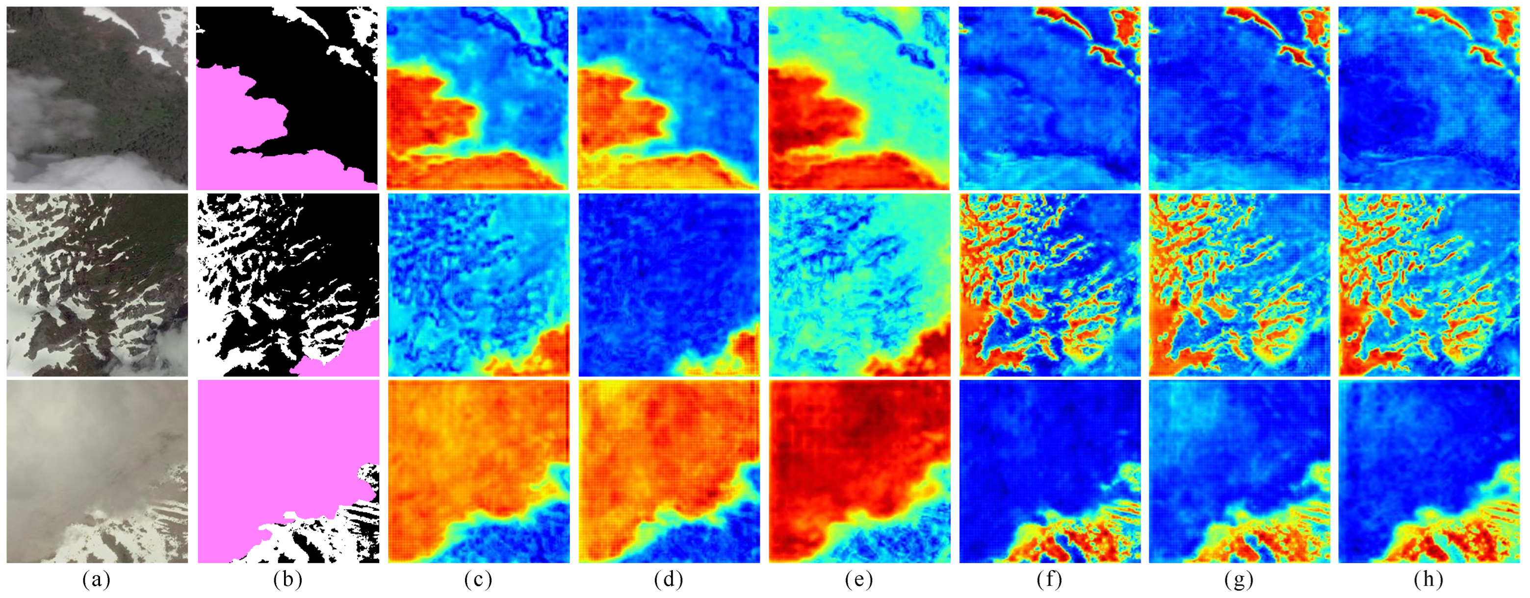
To further validate the role of DFE and DMIE, we input 3 images and used the heatmap to represent the changes of the output cloud and snow feature map under the corresponding module. For DFE, Figure 12d,e represent the cloud characteristic map with the DFE module and without the DFE module. Figure 12g,h represent the snow characteristic map with the DFE module and without the DFE module. We found that the output feature mapping with the DFE module was more focused on the key area and had richer boundary information. It showed that the DFE module can extract high-frequency detail features more effectively and has higher prediction accuracy for the boundary outline of cloud and snow, which is crucial to the regional positioning of restored images.
For DMIE, Figure 12c,f represent the cloud characteristic map and snow characteristic map with the DMIE module added. DMIE provided more-refined local features while preserving the detailed features of DFE and made up for part of the lost information. At the same time, the activated area was larger, and the relationship between features was mined more deeply, which enhanced the long-distance feature dependence. This indicated that the feature representation learned by the module had higher discriminative power.

3.4. Comparison Test of CSWV Dataset

To assess MAINet’s performance, we compare it to other models in this section. We chose the PA, harmonic mean (F1), Mean Pixel Accuracy (MPA), and MIoU as the assessment indicators of the experiment, and the specific outcomes of several methods in the same setting are shown in Table 3. Among all the methods, it was evident that the ResNet50-based MAINet had the best effect. MAINet without pretraining was superior to the other excellent segmentation methods without pretraining and was ahead of the pretrained PAN, FCN8sAtOnce, and PSPNet models. MAINet with no pretraining achieved 94.53%, 94.01%, 94.35%, and 88.71% on the PA, F1, MPA, and MIoU. After loading the pretrained model, the indexes of the PA, F1, MPA, and MIoU of our network were further improved to 95.51%, 94.99%, 95.21%, and 90.50%, surpassing the second place by 1.07%, 1.04%, 1.33%, and 1.9%, respectively. The performance of CvT using the method of introducing convolution into ViT is the worst in Table 3, while our model, MAINet, introduces the Transformer structure into the CNN in the DMIE module and combines the two in depth through bridging unit connections. This means that the network can naturally inherit the structural advantages of CNNs and Transformers and preserves the greatest extent of the ability to extract local and global properties, which greatly enhances both the representation ability of the network and the effectiveness of semantic segmentation. From the results of the evaluation indicators, it can be shown that the MAINet model well maintained the advantages of Transformers and achieved a good combination of CNNs. The effectiveness of our suggested method is shown by all these results.
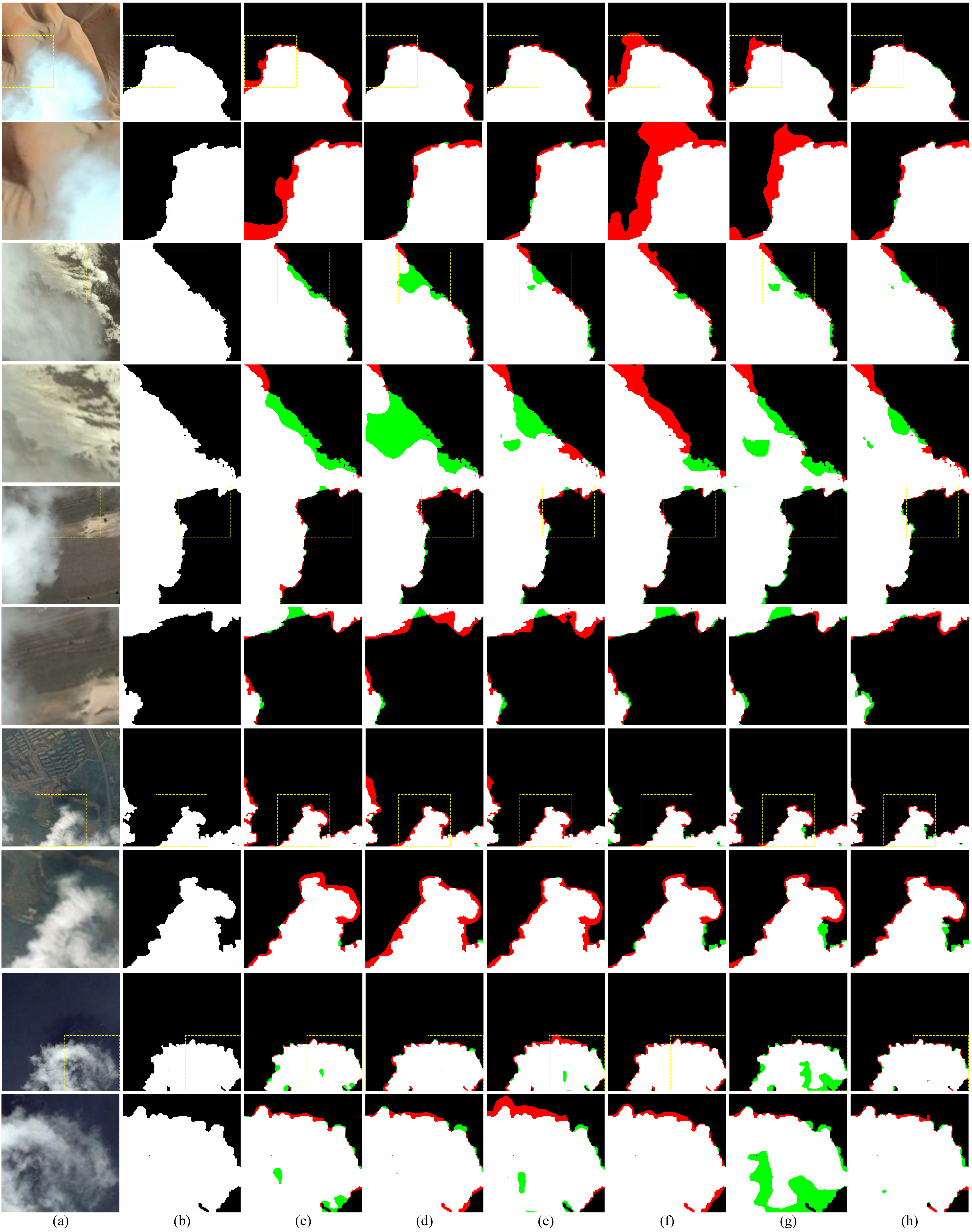
As shown in Figure 13, we selected the six models with the highest MIoU and selected six test images as the input to obtain the corresponding prediction results. By contrasting the predictions from several models, the performance of MAINet in cloud and snow segmentation can be better demonstrated visually. Since PSPNet uses the pyramid pooling module, it has more advantages in the field of global acceptance; however, the boundary of cloud and snow, the fragmented regions, and other details cannot be predicted well by PSPNet. This is because PSPNet loses much detail information after repeated down-sampling and the model does not have branches connected across layers to make up the features, so it is not dominant in detail. As can be seen from Figure 13d, PSPNet can only predict the approximate outline of the target with very rough details. Other multi-branch networks such as the FCN8S, CSDNet, PAN, and UNet can preserve some details to make the segmentation of cloud and snow edges more accurate. However, when the cloud layer is shallow, there are still some situations that cannot distinguish the cloud and the background, which cannot meet the fine requirements. In MAINet, the FIFU module we designed can better solve this problem, in which MSCB filters the shallow information, further obtains the multi-scale semantics, and strengthens the extraction of the boundary features. SCA enhances the spatial and channel information in the deep information and improves the robustness of the model, which is essential for enhancing segmentation accuracy. Finally, SFIF enhances the interaction ability between two channels, enhances the mutual connection, integrates the element representation of the two types, suppresses the weight of useless information, and integrates the context information in detail. With this operation, category false detection is significantly less likely to occur, and the accuracy of information throughout the up-sampling process is enhanced.
Furthermore, the fourth, fifth, and sixth lines in Figure 13 show that the detection results of the FCN8s, PANet, CSDNet, PSPNet, and UNet are prone to misdetect that the shaded snowy ground is classified as cloud, misdetect that the shaded snowy ground is classified as background, and ignore the discontinuous fine cloud pixels at the cloud boundary. There was a clear miscalculation of thin cloud and fine snow areas. According to Figure 13h, our MAINet network accurately segmented cloud and snow, correctly identified some obscure thin cloud areas, solved the problems existing in other algorithms, and improved the segmentation accuracy. The DFE we designed in MAINet fully preserved the detailed information in the down-sampling process, which contained a rich spatial position relationship between cloud and snow. The deep features were then guided by the FIFU module in up-sampling, effectively recovering the spatial position of each pixel. The result was that our model was better able to retain detailed information and extract the detailed features of cloud and snow, which proved the overall grasp of the detected images by our network.

3.5. Generalization Experiment

The approach was expanded to cloud detection to test MAINet’s capacity to generalize further. We utilized the HRC_WHU dataset as the training data, and the same networks in Section 3.4 were used to compare with our network based on the same experimental setup. We assessed the outcomes of the models by using the PA, F1, MPA, and MIoU as evaluation indicators. The outcome is displayed in Table 4. MAINet outperformed the other models on the HRC_WHU dataset in all indicators. It reached 95.60%, 94.82%, 95.64%, and 91.39% on the PA, F1, MPA, and MIoU, which were 0.38%, 0.42%, 0.34%, and 0.70% greater than the suboptimal PAN, respectively.
According to Figure 14, the other models had poor segmentation results with rough split edges, the severe loss of boundary details, and inaccurate positioning of thin clouds. MAINet deeply excavated the important relationship between the feature information by combining the CNN and Transformer structure through DMIE, realized the enhancement of high-frequency detail information, and made up for the loss of information in down-sampling with the help of MDIA. Through FIFU, the information from various scales was efficiently combined, the details of the segmentation boundary were enriched in the process of up-sampling and recovering the image, and the accurate positioning of the cloud layer was realized. The proposed model achieved the best segmentation result, which was beyond the reach of the other models. Our model more finely divided the cloud boundary at fragmented thin clouds, and the likelihood of erroneous detection at the boundary was significantly reduced, which can well adapt to segmentation tasks in different types of ground backgrounds. This result demonstrated that MAINet was more precise than the rival methods in estimating cloud cover and had higher generalization ability, which has practical significance in remote sensing applications.

4. Discussion

4.1. Advantages of the Proposed Method

This study proposed a ResNet-based encoder–decoder network structure method to overcome the problem. Compared with other works, the innovation of this model is that it reduces information loss and enhances detailed information through the DFE module in the down-sampling stage; uses the FIFU module in the feature fusion stage to improve the network structure and introduce channel space attention; uses in the deep layers the DMIE module, which adds operations such as the Transformer module to enhance the representation capabilities of the network. Additionally, the dataset we used to train our model included images from tropical, temperate, and cold regions. For situations in tropical climates where cloud cover can be persistent and variable, the model’s ability to accurately segment clouds contributes to its utility in understanding and managing tropical ecosystems. In temperate climates with significant seasonal changes, the model performed well in cloud and snow segmentation, which is important for assessing water resources, understanding snowmelt dynamics, and predicting potential flooding events. In cold climates characterized by long-term snow cover, our model proved particularly useful for monitoring changes in snow cover distribution and extent. Our model’s accurate segmentation of snowpack facilitates climate research related to albedo changes and permafrost dynamics. The successful application of its detection results in different climatic environments highlights its potential to provide valuable insights into remote sensing and environmental monitoring.

4.2. Limitations and Future Research Directions

While our deep learning model achieved significant results in cloud and snow segmentation in remote sensing images, there are still limitations that need further discussion. The acquisition of remote sensing images involves various methods, including Synthetic Aperture Sonar (SAS) and Synthetic Aperture Radar (SAR). The features of these images differ from those used in this study, which may affect the performance of our approach. Future research directions could involve experimenting with other types of remote sensing images. We might need to perform specific preprocessing on the input images or adjust our network architecture and parameters to increase the model’s applicability. Furthermore, the model may perform poorly when dealing with cloud and snow cover under extreme weather conditions. The reason could be the lack of samples representing extreme conditions in the training dataset, preventing the model from adequately capturing features in such situations. Improving the model’s robustness can be addressed in future work by augmenting the dataset with samples that represent these special cases.

5. Summary

Accurate cloud and snow recognition can improve the application of optical satellite data and, also, has high application value in weather forecasting, climate observations, and so on. This paper introduced an encoder–decoder network called Multi-level Attention Interactive Network for cloud and snow detection segmentation. The proposal of MAINet solves to a certain extent the defects of certain missing features and some false detections in the results of previous detection methods and is suitable for medium- and high-resolution images in the visible wavelengths:
  • Some contributions adopted in MAINet’s structure:
    MAINet utilizes an encoder–decoder network with ResNet50 as the backbone, which mines semantic data at various levels.
    The DMIE module combines the CNN and Transformer features to deeply mine rich feature information.
    The DFE module compensates for the detailed semantic information that was lost during the encoder’s down-sampling process.
    In the FIFU module, SFIF performs two-channel fusion. For information communication, CSAM enhances the deep spatial channel information, and MSBC enhances the peripheral information and feature information of the segmentation boundaries.
The experimental results showed that our proposed MAINet outperformed other algorithms on the CSWV and HRC_WHU datasets, and the PA, F1, MPA, and MIoU indicators reached 95.51%, 94.99%, 95.21%, and 90.50% and 95.60%, 94.82%, 95.64%, and 91.39%, respectively. MAINet considerably increased the accuracy of detection in comparison to the previous methods and achieved better segmentation results in various complex scenes, with very good generalization and robustness.

Author Contributions

Conceptualization, L.D. and M.X.; methodology, M.X. and K.H.; software, L.D.; validation, K.H. and H.L.; formal analysis, M.X. and H.L.; investigation, L.D. and H.L.; resources, M.X. and K.H.; data curation, L.D.; writing—original draft preparation, L.D.; writing—review and editing, M.X.; visualization, L.D.; supervision, M.X.; project administration, M.X.; funding acquisition, M.X. All authors have read and agreed to the published version of the manuscript.

Funding

This work is supported in part by the National Natural Science Foundation of PR China (42075130).

Data Availability Statement

The data sets of CSWV and HRC_WHU are publicly available https://github.com/zhanggb1997/CSDNet-CSWV and http://sendimage.whu.edu.cn/en/hrc_whu/ respectively.

Conflicts of Interest

The authors declare no conflicts of interest.

References

  1. Cohen, W.B.; Fiorella, M.; Gray, J.; Helmer, E.; Anderson, K. An efficient and accurate method for mapping forest clearcuts in the Pacific Northwest using Landsat imagery. Photogramm. Eng. Remote Sens. 1998, 64, 293–299. [Google Scholar]
  2. Kattenborn, T.; Leitloff, J.; Schiefer, F.; Hinz, S. Review on Convolutional Neural Networks (CNN) in vegetation remote sensing. ISPRS J. Photogramm. Remote Sens. 2021, 173, 24–49. [Google Scholar] [CrossRef]
  3. Zhu, Z.; Woodcock, C.E. Automated cloud, cloud shadow, and snow detection in multitemporal Landsat data: An algorithm designed specifically for monitoring land cover change. Remote Sens. Environ. 2014, 152, 217–234. [Google Scholar] [CrossRef]
  4. Chen, K.; Dai, X.; Xia, M.; Weng, L.; Hu, K.; Lin, H. MSFANet: Multi-Scale Strip Feature Attention Network for Cloud and Cloud Shadow Segmentation. Remote Sensing 2023, 15, 4853. [Google Scholar] [CrossRef]
  5. Campos, N.; Quesada-Román, A.; Granados-Bolaños, S. Mapping Mountain Landforms and Its Dynamics: Study Cases in Tropical Environments. Appl. Sci. 2022, 12, 10843. [Google Scholar] [CrossRef]
  6. Quesada-Román, A.; Umaña-Ortíz, J.; Zumbado-Solano, M.; Islam, A.; Abioui, M.; Zangmo Tefogoum, G.; Kariminejad, N.; Mutaqin, B.W.; Pupim, F. Geomorphological regional mapping for environmental planning in developing countries. Environ. Dev. 2023, 48, 100935. [Google Scholar] [CrossRef]
  7. Klein, A.G.; Hall, D.K.; Riggs, G.A. Improving snow cover mapping in forests through the use of a canopy reflectance model. Hydrol. Process. 1998, 12, 1723–1744. [Google Scholar] [CrossRef]
  8. Quesada-Román, A.; Peralta-Reyes, M. Geomorphological Mapping Global Trends and Applications. Geographies 2023, 3, 610–621. [Google Scholar] [CrossRef]
  9. Qiu, S.; Zhu, Z.; He, B. Fmask 4.0: Improved cloud and cloud shadow detection in Landsats 4–8 and Sentinel-2 imagery. Remote Sens. Environ. 2019, 231, 111205. [Google Scholar] [CrossRef]
  10. Gladkova, I.; Shahriar, F.; Grossberg, M.; Frey, R.A.; Menzel, W.P. Impact of the aqua MODIS Band 6 restoration on cloud/snow discrimination. J. Atmos. Ocean. Technol. 2013, 30, 2712–2719. [Google Scholar] [CrossRef]
  11. Haiyan, D.; Lingling, M.; Ziyang, L.; Lingli, T. Automatic identification of cloud and snow based on fractal dimension. Remote Sens. Technol. Appl. 2013, 28, 52–57. [Google Scholar]
  12. Zhu, Z.; Wang, S.; Woodcock, C.E. Improvement and expansion of the Fmask algorithm: Cloud, cloud shadow, and snow detection for Landsats 4–7, 8, and Sentinel 2 images. Remote Sens. Environ. 2015, 159, 269–277. [Google Scholar] [CrossRef]
  13. Wang, J.; Li, W. Comparison of methods of snow cover mapping by analysing the solar spectrum of satellite remote sensing data in China. Int. J. Remote Sens. 2003, 24, 4129–4136. [Google Scholar] [CrossRef]
  14. Vapnik, V.N. An overview of statistical learning theory. IEEE Trans. Neural Netw. 1999, 10, 988–999. [Google Scholar] [CrossRef]
  15. Belgiu, M.; Drăguţ, L. Random forest in remote sensing: A review of applications and future directions. ISPRS J. Photogramm. Remote Sens. 2016, 114, 24–31. [Google Scholar] [CrossRef]
  16. Hollstein, A.; Segl, K.; Guanter, L.; Brell, M.; Enesco, M. Ready-to-use methods for the detection of clouds, cirrus, snow, shadow, water and clear sky pixels in Sentinel-2 MSI images. Remote Sens. 2016, 8, 666. [Google Scholar] [CrossRef]
  17. Hughes, M.J.; Hayes, D.J. Automated detection of cloud and cloud shadow in single-date Landsat imagery using neural networks and spatial post-processing. Remote Sens. 2014, 6, 4907–4926. [Google Scholar] [CrossRef]
  18. Sun, L.; Cao, X. Feature extraction based on combined textural features from panchromatic cloud and snow region. Electron. Design Eng. 2014, 22, 174–176. [Google Scholar]
  19. Ghasemian, N.; Akhoondzadeh, M. Introducing two Random Forest based methods for cloud detection in remote sensing images. Adv. Space Res. 2018, 62, 288–303. [Google Scholar] [CrossRef]
  20. Kang, X.; Gao, G.; Hao, Q.; Li, S. A coarse-to-fine method for cloud detection in remote sensing images. IEEE Geosci. Remote Sens. Lett. 2018, 16, 110–114. [Google Scholar] [CrossRef]
  21. Chai, D.; Newsam, S.; Zhang, H.K.; Qiu, Y.; Huang, J. Cloud and cloud shadow detection in Landsat imagery based on deep convolutional neural networks. Remote Sens. Environ. 2019, 225, 307–316. [Google Scholar] [CrossRef]
  22. Jeppesen, J.H.; Jacobsen, R.H.; Inceoglu, F.; Toftegaard, T.S. A cloud detection algorithm for satellite imagery based on deep learning. Remote Sens. Environ. 2019, 229, 247–259. [Google Scholar] [CrossRef]
  23. Dai, X.; Chen, K.; Xia, M.; Weng, L.; Lin, H. LPMSNet: Location Pooling Multi-Scale Network for Cloud and Cloud Shadow Segmentation. Remote Sens. 2023, 15, 4005. [Google Scholar] [CrossRef]
  24. Ji, H.; Xia, M.; Zhang, D.; Lin, H. Multi-Supervised Feature Fusion Attention Network for Clouds and Shadows Detection. ISPRS Int. J. Geo-Inf. 2023, 12, 247. [Google Scholar] [CrossRef]
  25. Dai, X.; Xia, M.; Weng, L.; Hu, K.; Lin, H.; Qian, M. Multi-Scale Location Attention Network for Building and Water Segmentation of Remote Sensing Image. IEEE Trans. Geosci. Remote Sens. 2023, 61, 5609519. [Google Scholar] [CrossRef]
  26. Lu, C.; Xia, M.; Qian, M.; Chen, B. Dual-Branch Network for Cloud and Cloud Shadow Segmentation. IEEE Trans. Geosci. Remote Sens. 2022, 60, 5410012. [Google Scholar] [CrossRef]
  27. Weng, L.; Pang, K.; Xia, M.; Lin, H.; Qian, M.; Zhu, C. Sgformer: A Local and Global Features Coupling Network for Semantic Segmentation of Land Cover. IEEE J. Sel. Top. Appl. Earth Obs. Remote Sens. 2023, 16, 6812–6824. [Google Scholar] [CrossRef]
  28. Zhan, Y.; Wang, J.; Shi, J.; Cheng, G.; Yao, L.; Sun, W. Distinguishing cloud and snow in satellite images via deep convolutional network. IEEE Geosci. Remote Sens. Lett. 2017, 14, 1785–1789. [Google Scholar] [CrossRef]
  29. Long, J.; Shelhamer, E.; Darrell, T. Fully convolutional networks for semantic segmentation. In Proceedings of the IEEE Conference on Computer Vision and Pattern Recognition, Boston, MA, USA, 7–12 June 2015; pp. 3431–3440. [Google Scholar]
  30. Xie, F.; Shi, M.; Shi, Z.; Yin, J.; Zhao, D. Multilevel cloud detection in remote sensing images based on deep learning. IEEE J. Sel. Top. Appl. Earth Obs. Remote Sens. 2017, 10, 3631–3640. [Google Scholar] [CrossRef]
  31. Zhang, G.; Gao, X.; Yang, Y.; Wang, M.; Ran, S. Controllably Deep Supervision and Multi-Scale Feature Fusion Network for Cloud and Snow Detection Based on Medium-and High-Resolution Imagery Dataset. Remote Sens. 2021, 13, 4805. [Google Scholar] [CrossRef]
  32. He, K.; Zhang, X.; Ren, S.; Sun, J. Deep residual learning for image recognition. In Proceedings of the IEEE Conference on Computer Vision and Pattern Recognition, Las Vegas, NV, USA, 1–26 July 2016; pp. 770–778. [Google Scholar]
  33. Lin, M.; Chen, Q.; Yan, S. Network in network. arXiv 2013, arXiv:1312.4400. [Google Scholar]
  34. Parmar, N.; Vaswani, A.; Uszkoreit, J.; Kaiser, L.; Shazeer, N.; Ku, A.; Tran, D. Image Transformer. In Proceedings of the International Conference on Machine Learning, PMLR, Stockholm, Sweden, 10–15 July 2018; pp. 4055–4064. [Google Scholar]
  35. Ioffe, S.; Szegedy, C. Batch normalization: Accelerating deep network training by reducing internal covariate shift. In Proceedings of the International Conference on Machine Learning, PMLR, Lille, France, 6–11 July 2015; pp. 448–456. [Google Scholar]
  36. Peng, Z.; Huang, W.; Gu, S.; Xie, L.; Wang, Y.; Jiao, J.; Ye, Q. Conformer: Local features coupling global representations for visual recognition. In Proceedings of the IEEE/CVF International Conference on Computer Vision, Montreal, BC, Canada, 11–17 October 2021; pp. 367–376. [Google Scholar]
  37. Dosovitskiy, A.; Beyer, L.; Kolesnikov, A.; Weissenborn, D.; Zhai, X.; Unterthiner, T.; Dehghani, M.; Minderer, M.; Heigold, G.; Gelly, S.; et al. An image is worth 16 × 16 words: Transformers for image recognition at scale. arXiv 2020, arXiv:2010.11929. [Google Scholar]
  38. Wu, B.; Xu, C.; Dai, X.; Wan, A.; Zhang, P.; Yan, Z.; Tomizuka, M.; Gonzalez, J.; Keutzer, K.; Vajda, P. Visual Transformers: Token-based image representation and processing for computer vision. arXiv 2020, arXiv:2006.03677. [Google Scholar]
  39. Zhu, X.; Su, W.; Lu, L.; Li, B.; Wang, X.; Dai, J. Deformable detr: Deformable Transformers for end-to-end object detection. arXiv 2020, arXiv:2010.04159. [Google Scholar]
  40. Zheng, S.; Lu, J.; Zhao, H.; Zhu, X.; Luo, Z.; Wang, Y.; Fu, Y.; Feng, J.; Xiang, T.; Torr, P.H.; et al. Rethinking semantic segmentation from a sequence-to-sequence perspective with Transformers. In Proceedings of the IEEE/CVF Conference on Computer Vision and Pattern Recognition, Nashville, TN, USA, 20–25 June 2021; pp. 6881–6890. [Google Scholar]
  41. Ba, J.L.; Kiros, J.R.; Hinton, G.E. Layer normalization. arXiv 2016, arXiv:1607.06450. [Google Scholar]
  42. Ronneberger, O.; Fischer, P.; Brox, T. U-net: Convolutional networks for biomedical image segmentation. In Medical Image Computing and Computer-Assisted Intervention—MICCAI 2015; Springer: Berlin/Heidelberg, Germany, 2015; pp. 234–241. [Google Scholar]
  43. Chen, B.; Xia, M.; Qian, M.; Huang, J. MANet: A multi-level aggregation network for semantic segmentation of high-resolution remote sensing images. Int. J. Remote Sens. 2022, 43, 5874–5894. [Google Scholar] [CrossRef]
  44. Liu, Y.; Shao, Z.; Teng, Y.; Hoffmann, N. NAM: Normalization-based Attention Module. arXiv 2021, arXiv:2111.12419. [Google Scholar]
  45. Dosovitskiy, A.; Springenberg, J.T.; Brox, T. Unsupervised feature learning by augmenting single images. arXiv 2013, arXiv:1312.5242. [Google Scholar]
  46. Li, Z.; Shen, H.; Cheng, Q.; Liu, Y.; You, S.; He, Z. Deep learning based cloud detection for medium and high resolution remote sensing images of different sensors. ISPRS J. Photogramm. Remote Sens. 2019, 150, 197–212. [Google Scholar] [CrossRef]
  47. Kingma, D.P.; Ba, J. Adam: A method for stochastic optimization. arXiv 2014, arXiv:1412.6980. [Google Scholar]
  48. Chen, L.C.; Papandreou, G.; Kokkinos, I.; Murphy, K.; Yuille, A.L. Deeplab: Semantic image segmentation with deep convolutional nets, atrous convolution, and fully connected crfs. IEEE Trans. Pattern Anal. Mach. Intell. 2017, 40, 834–848. [Google Scholar] [CrossRef] [PubMed]
  49. Zhao, H.; Shi, J.; Qi, X.; Wang, X.; Jia, J. Pyramid scene parsing network. In Proceedings of the IEEE Conference on Computer Vision and Pattern Recognition, Honolulu, HI, USA, 21–26 July 2017; pp. 2881–2890. [Google Scholar]
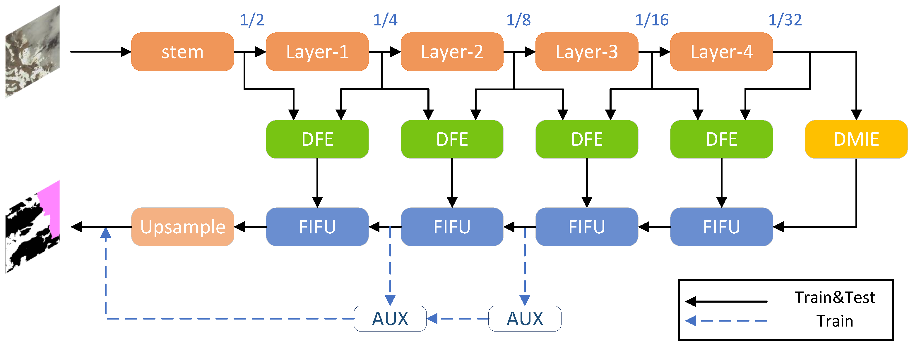
Figure 1. The architecture of MAINet consists of a backbone and three modules. ResNet50 preliminary extracts the features, and the deep semantic features are further extracted by DMIE. Then, DFE is used to establish the skip connections and extract guidance information, and FIFU is used to complete the up-sampling feature fusion and position recovery. Finally, bilinear up-sampling operation is used to output the prediction results. During training, the AUX is added as extra output to speed up the training efficiency.
Remotesensing 16 00112 g001
Figure 2. The structure of the AUX.
Remotesensing 16 00112 g002
Figure 3. (a) The overall structure of Deep Multi-head Information Enhancement. (b) The bottompart of the BCM. (c) The toppart of the BCM.
Remotesensing 16 00112 g003
Figure 4. The structure of Transformer block.
Remotesensing 16 00112 g004
Figure 5. The structure of Detail Feature Extraction.
Remotesensing 16 00112 g005
Figure 6. The structure of Feature Interaction and Fusion Up-sampling.
Remotesensing 16 00112 g006
Figure 7. The structure of multi-scale and strip boundary convolution.
Remotesensing 16 00112 g007
Figure 8. (a) Spatial channel attention (b) SpatialAttention block (c) ChannelAttention block.
Remotesensing 16 00112 g008
Figure 9. The structure of Spatial Feature Interactive Fusion.
Remotesensing 16 00112 g009
Figure 10. Some of the training data in CSWV. (a) The original image of CSWV. (b) The corresponding pixel label. The pink represents clouds, the white snow, and the black the background.
Remotesensing 16 00112 g010
Figure 11. Some of the training data in HRC_WHU. (a) The original image of HRC_WHU. (b) The corresponding pixel label. The white represents clouds, and the black represents the background.
Remotesensing 16 00112 g011
Figure 12. Heatmap representation. (a) Test image; (b) labels; (c) cloud feature with DFE and DMIE; (d) cloud feature with DFE; (e) cloud feature without DFE and DMIE; (f) snow feature with DFE and DMIE; (g) snow feature with DFE; (h) snow feature without DFE and DMIE.
Remotesensing 16 00112 g012
Figure 13. The prediction of different models on CSWV dataset. (a) The original images; (b) labels; (c) FCN8s; (d) PSPNet; (e) CSDNet; (f) PANet; (g) UNet; (h) MAINet. The red areas are error detection. The green areas are misdetection. The yellow dotted box area is enlarged below each image.
Remotesensing 16 00112 g013
Figure 14. The prediction of different models on the HRC_WHU dataset. (a) The original images; (b) labels; (c) DeepLabV3Plus; (d) PSPNet; (e) PAN; (f) ACFNet; (g) OCRNet; (h) MAINet. The red areas are error detection. The green areas are misdetection. The yellow dotted box area is enlarged below each image.
Remotesensing 16 00112 g014
Table 1. Setting the AUX branch.
MethodAUXPA (%)MIoU (%)Parameter (M)Flops (G)
ResNet5095.5190.5013.8160.66
ResNet5094.7688.9113.3560.43
Table 2. Ablation experiments of MAINet.
MethodPA (%)MIoU (%)Parameter (M)Flops (G)
ResNet5094.3788.1838.8610.82
ResNet50+SCA94.8189.1842.0111.36
ResNet50+SCA+SFIF95.0189.5242.0111.37
ResNet50+SCA+SFIF+MSBC95.1089.7143.0812.34
ResNet50+SCA+SFIF+MSBC+DFE95.2890.0944.1312.75
ResNet50+SCA+SFIF+MSBC+DFE+DMIE95.5190.5060.6613.81
Table 3. Results on CSWV dataset. Pretrained models are marked with ‘†’ (bold represents the best).
MethodPA (%)F1 (%)MPA (%)MIoU (%)
CvT89.7188.1188.3678.84
DeepLabV3Plus91.1689.7790.2681.63
HRNet91.4990.3890.5182.46
SegNet91.6490.6591.3582.85
OCRNet92.0290.4991.3083.52
CGNet91.9891.0891.4783.67
DABNet91.9791.1591.4083.68
FCN8s91.8991.1491.6883.74
ACFNet92.3491.4291.7384.21
PSPNet92.5191.7091.9884.71
PAN92.6691.9192.3785.05
DFN93.2392.5392.1086.22
CSDNet93.7893.1093.7187.08
UNet93.9493.4594.3187.60
MAINet94.5394.0194.3588.71
PAN †93.8393.2793.7787.39
FCN8s †94.1193.5693.0087.83
PSPNet †94.4493.9593.8888.60
MAINet †95.5194.9995.2190.50
Table 4. Results on HRC_WHU dataset. Pretrained models are marked with ‘†’ (bold represents the best).
MethodPA (%)F1 (%)MPA (%)MIoU (%)
CvT93.4192.1893.2687.36
CGNet93.9893.0394.1988.45
FCN8s94.2193.1194.0488.80
HRNet94.3093.2094.1188.95
UNet94.3493.3694.3989.07
PAN94.3993.3594.3089.14
CSDNet94.3993.4594.5189.17
DABNet94.5393.5894.5589.42
SegNet94.5893.5994.5189.50
PSPNet94.5993.6594.6289.53
DFN94.6493.7394.7489.63
DeepLabV3Plus94.8493.9794.9489.99
ACFNet94.8894.0295.0090.07
OCRNet95.1394.2094.9790.49
MAINet95.3494.5495.4290.91
FCN8s †94.7393.8094.7489.77
PSPNet †94.9093.9794.8690.08
PAN †95.2294.4095.3090.69
MAINet †95.6094.8295.6491.39
Disclaimer/Publisher’s Note: The statements, opinions and data contained in all publications are solely those of the individual author(s) and contributor(s) and not of MDPI and/or the editor(s). MDPI and/or the editor(s) disclaim responsibility for any injury to people or property resulting from any ideas, methods, instructions or products referred to in the content.