Article

Dynamic Evolution and Scenario Simulation of Ecosystem Services under the Impact of Land-Use Change in an Arid Inland River Basin in Xinjiang, China

1
College of Geography and Remote Sensing Sciences, Xinjiang University, Urumqi 830046, China
2
State Key Laboratory of Desert and Oasis Ecology, Xinjiang Institute of Ecology and Geography, Chinese Academy of Sciences, Urumqi 830011, China
3
University of Chinese Academy of Sciences, Beijing 100049, China
*
Author to whom correspondence should be addressed.
Remote Sens. 2023, 15(9), 2476; https://doi.org/10.3390/rs15092476
Submission received: 10 March 2023 / Revised: 24 April 2023 / Accepted: 4 May 2023 / Published: 8 May 2023

Abstract

:
Ecosystem services (ESs) are crucial for sustainable development, as they impact human well-being. However, changes in land use/land cover (LULC) caused by climate change and social development can negatively affect ESs, particularly in arid river basins. This study focuses on current and future changes in LULC in the Kaxghar River Basin (KRB) in Xinjiang, China, to determine how these changes will affect the region’s ESs. The integrated PLUS-InVEST model was used to investigate the spatiotemporal distribution and changing patterns of habitat quality (HQ) and carbon storage (CS) under the natural increase scenario (NIS), economic development scenario (EDS), and water protection scenario (WPS). Additionally, the Ecosystem Service Contribution Index (ESCI) was also calculated to evaluate the contribution of LULC changes to ESs. The results show the following: (1) from 2000 to 2020, the average value of HQ in the KRB gradually decreased from 0.54 to 0.49 and CS trended slightly upward, with a total increase of 0.07 × 10⁶ t. Furthermore, the changes in CS were highly consistent with changes in LULC. (2) From 2020 to 2030, the area of low-grade (0–0.2) HQ saw a continuous increase, with the fastest growth occurring in 2030 under the EDS. Meanwhile, under the WPS, HQ significantly improved, expanding by 1238 km2 in area. Total CS under the three test scenarios tended to decline, with the NIS showing the smallest decrease. (3) The expansion of cropland and unused land had a negative impact on ESs, particularly on CS, whereas the conversion to grassland and forestland had a significant positive impact. In conclusion, these insights will enrich our understanding of ESs in the study area and contribute to balancing the relationship between ecological conservation and socioeconomic development in the Kaxghar River Basin, as well as in other parts of China’s arid Northwest and similar regions around the world.

Graphical Abstract

1. Introduction

The natural ecosystem is crucial for human survival and development [1], as it provides resources and materials necessary for life [2] and maintains a balance between humans and nature [3]. This ability, which is known as ecosystem services (ESs), includes provisioning, regulating, supporting, and cultural services [4,5]. Land use/land cover (LULC) is the primary factor affecting ESs [6], serving as a link between human activities and ecological processes [7]. Changes in LULC, such as the conversion of forestland and grassland to cropland and built-up land, significantly alter the structure and function of ESs [8,9], leading to ecosystem imbalances and subsequent reductions in human well-being [10]. These impacts are more pronounced in ecologically fragile areas [11], making the assessment of ESs based on land-use changes in these areas crucial for enhancing ecological security and improving ecological benefits.
Numerous methods have been used over the years to assess ecosystem services [12], with several models being developed for ES valuation. Among them, the InVEST model has the advantage of integrating and quantifying multiple ESs [13]. It has been widely used in ES research [14,15], including for evaluations [16], supply and demand changes [17], trade-offs/synergies [18], and drivers [19,20] of ESs. For instance, Ma et al. [21] studied the spatiotemporal changes in ESs in the conservation-priority regions of China. The researchers in [22] conducted a case study on the urban agglomeration of the Chaobai River in northern China, analyzing the relationship between the supply and demand of ESs and proposing a research scheme for ES protection and management. The spatiotemporal variations in water-related ESs were assessed in [23], with the authors identifying trade-offs between food production and water-related ESs in the Songhua River Basin. Additionally, some studies assessed changes in a specific type of ES, such as carbon storage [24], water conservation [25], and habitat quality [26].
Currently, research on how land-use change affects ESs is a hot topic in ecology and geography [27,28,29]. Li et al. [30] studied the effects of land-use change on ESs in the China–Mongolia–Russia Economic Corridor and found that these changes had significant impacts on ESs, indicating that it is crucial to further examine future trends in ESs that are driven by human activities. Accordingly, to estimate changes in ESs, the InVEST model was combined with future land-use scenario simulation strategies, such as the CA-Markov [31], FLUS [32], and CLUE-S [33]. While these models were able to provide satisfactory predictions, they were unable to offer insights into the dynamics behind transitions of individual land-use types and their impact on expected changes, as pointed out by Liang [34].
To address this limitation, the Patch-generating Land-Use Simulation (PLUS) model has been developed based on the Cellular Automata (CA) model [35]. PLUS integrates two main components: a rule-mining framework that explores transformation rules using the Land Expansion Analysis Strategy (LEAS) and a CA model based on multitype Random Seeds (CARS). This integration has improved the ability to simulate land-use changes and their impacts, as demonstrated by Wang et al. [36], making the PLUS model a promising tool for investigating future land-use scenarios [19,37].
The KRB is one of the most important tributaries of the TRB in Northwest China. In recent years, however, the KRB has lost its surface water connection with the TRB mainstream due to climate change and increasing agricultural activities [38,39]. This loss has led to a range of ecological issues, including land desertification, water scarcity and pollution, reduced biodiversity, and heightened vulnerability to natural disasters, such as droughts and sandstorms. The result has been a rapid decline in ESs in the KRB [40], directly threatening the ecological security of the region.
Considering the seriousness of these recent changes, it is prudent to conduct research on the ESs in the KRB to find ways to improve the ecological environment and promote sustainable regional economic development. The research gap on dynamic changes in the KRB’s LULC and how these changes may affect ESs in the future urgently needs to be addressed. Therefore, the current study focuses on the two key ecosystem services of habitat quality (HQ) and carbon storage (CS) and aims to investigate the spatiotemporal distribution and changing patterns of these ESs. It also attempts to quantify the contribution of LULC changes to ESs under future scenarios using the integrated InVEST-PLUS model. The results of this study can provide a scientific basis for land-use planning and the sustainable development of ecosystems in arid regions.

2. Materials and Methods
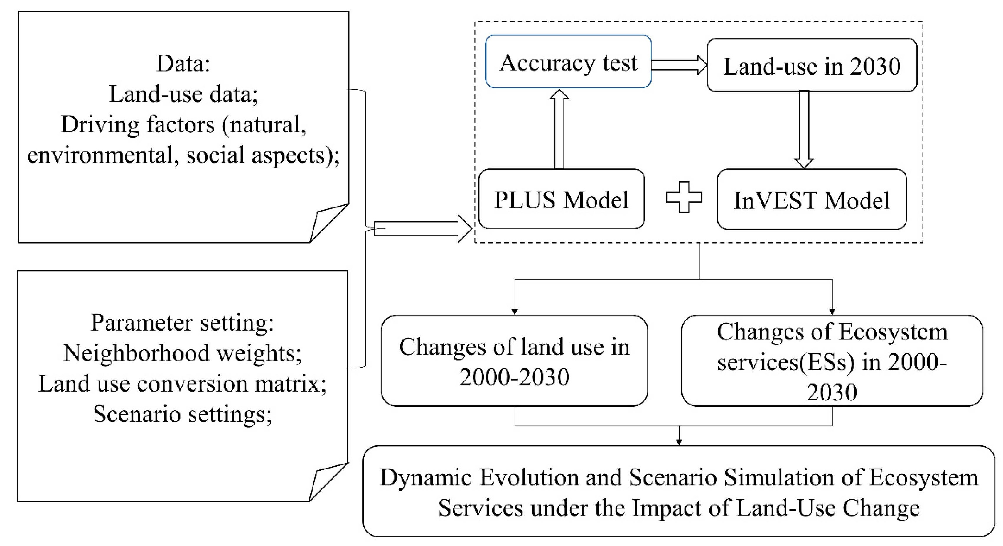
2.1. Study Area

The Kaxghar River Basin (KRB) (73°03′~80°25′E, 38°10′~40°55′N) is located on the western edge of the Tarim River Basin (TRB) in China’s arid Northwest. It is surrounded by mountains to the north, south, and west and flat terrain to the east. As one of the main headwaters of the Tarim river, the KRB encompasses six rivers and covers an area of approximately 7.2 × 10⁴ km2. The altitude varies significantly across the basin, averaging around 1298 m and falling rapidly from the west to the east. The continental arid climate in the KRB is characterized by sparse precipitation, intense evaporation, ample sunlight, large temperature differences between day and night, short winters, and long summers. There is little interannual variation in temperature in the basin, with an average annual temperature of 11.7 °C, annual rainfall of 137.4 mm, and potential evaporation of more than 3000 mm [41]. The study area is depicted in Figure 1.

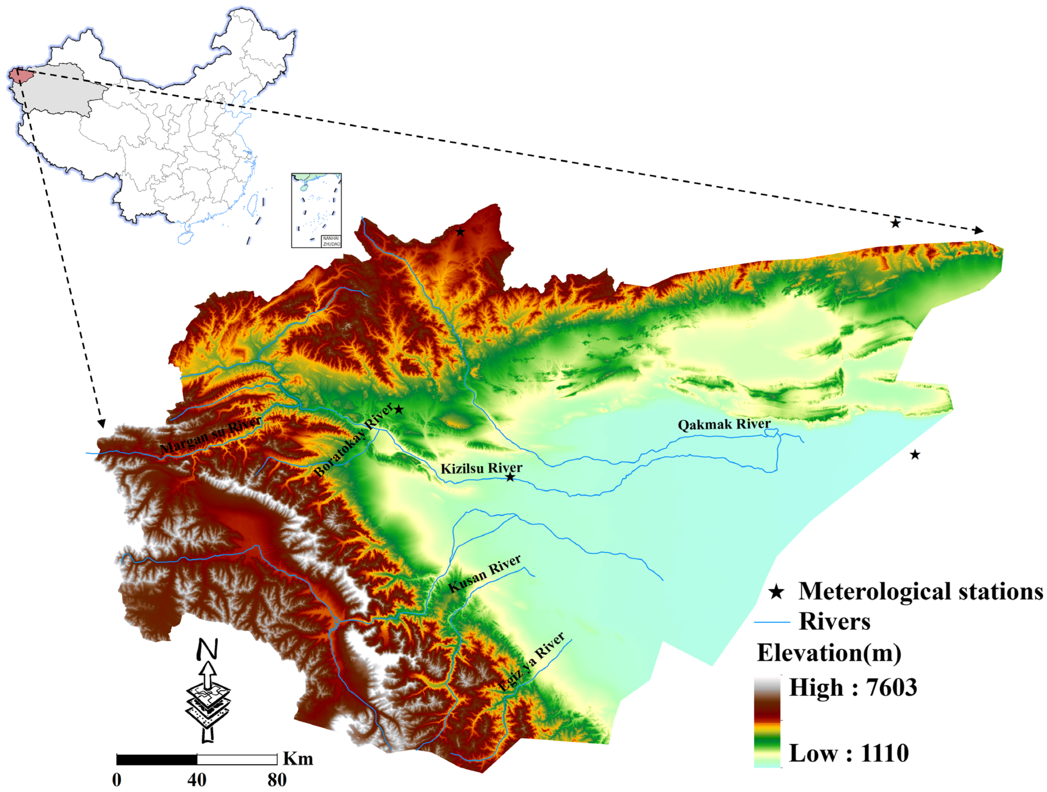
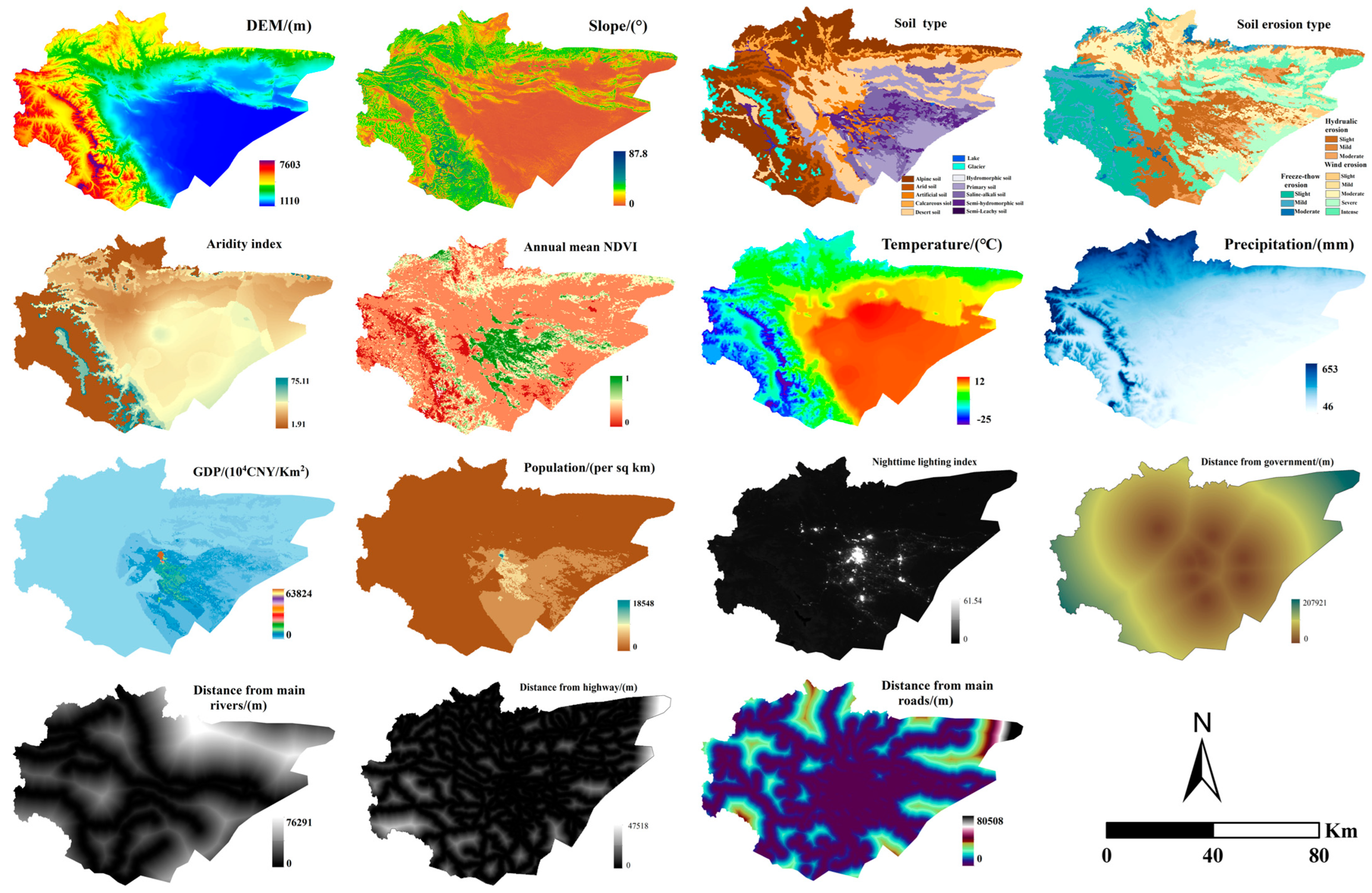
2.2. Materials and Data Processing
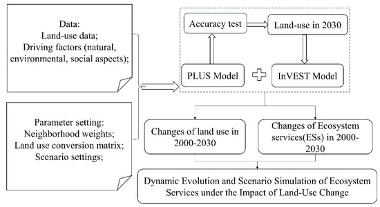
Land use/land cover data with a 30 m spatial resolution for 2000, 2010, and 2020 were collected from the Chinese Academy of Sciences (CAS) (https://www.resdc.cn/data.aspx, accessed on 20 June 2022). Fifteen driving factors were selected for this study, including seven natural and environmental factors and eight socioeconomic factors that significantly affect land-use change. Among the seven natural and environmental factors, five (the aridity index, erosion intensity, soil type, annual mean temperature, and precipitation [1 km × 1 km]) were collected from the Center for Resource and Environmental Science Data, CAS (https://www.resdc.cn/, accessed on 20 June 2022), while the Digital Elevation Model (DEM) with a resolution of 30 m was collected from the Geospatial data cloud (http://www.gscloud.cn/, accessed on 20 June 2022), and the slope factor was derived from DEM using ArcGIS10.6.
The eight socioeconomic factors included population density, GDP, normalized difference vegetation index (NDVI), Nighttime Light Index (NLI), and distance variables, such as distance from government, rivers, main roads, and highways. The 1 km gridded population density and GDP were obtained from CAS (https://www.resdc.cn/data.aspx). NDVI data were derived from MODIS MOD13Q1, with a spatial resolution of 250 m, produced by the NASA EOS data center (https://ladsweb.modaps.eosdis.nasa.gov, accessed on 20 June 2022). NLI data with a spatial resolution of 500 m were collected from the VIIRS_DNB_VNLV2 datasets of the earth observation group (EOG) (https://eogdata.mines.edu, accessed on 20 June 2022). In this study, the Google Earth Engine (GEE) platform was employed to collect and process the NDVI and NLI imagery. Distance variables were obtained from the open street map (https://www.openstreetmap.org, accessed on 20 June 2022) and were calculated in ArcGIS 10.6 using the Euclidean distance. After a series of data pretreatment steps, such as projection transformation, clipping, and resampling in ArcGIS10.6 software, all drivers were converted into the same projection of WGS-1984-UTM zone-45N, at a resolution of 30 m × 30 m (Figure 2).

2.3. Methodology

The main objective of this study was to predict spatiotemporal changes in land use/land cover and their impact on ecosystem services under various scenarios in the KRB. As presented in Figure 3, the research conducted in this study was divided into several steps. First, an analysis was performed on the spatiotemporal distribution characteristics of LULC in the KRB. Secondly, the InVEST model was utilized to evaluate the dynamic changes in HQ and CS ecosystem services. Thirdly, the PLUS model was employed to predict the land-use distribution in 2030 under different scenarios, and the spatial distribution of the aforementioned ESs was further analyzed. Finally, an ES index was calculated to assess the impact of different land-use changes on ESs.

2.3.1. Assessment of Habitat Quality

Habitat quality is an important factor in the conservation of biodiversity and the sustainable development of regions [32]. The evaluation of HQ relies on several crucial parameters, with the three main ones being as follows: (1) the identification of potential threats to HQ and their distance from habitats, (2) the sensitivity of each LULC type to each threat, and (3) the suitability of each LULC type to provide a habitat. The InVEST model produces an HQ map showing the HQ value range from 0 to 1, with a higher HQ value indicating better habitat quality and greater biodiversity [42]. Areas of intensive human activity, including cropland, built-up land, and unused land, are considered threat factors [43] based on the conditions in the study area. Different LULC types exhibit varying degrees of sensitivity to threat sources, which are primarily determined by ecological and landscape ecology theories, as well as biodiversity conservation principles [44].
The main principle of the habitat quality assessment module is to establish a relationship between land use and threat sources [45]. To do so, habitat distribution is calculated based on the response of different habitats to threat sources, while the sensitivity of each LULC type to threat sources is considered based on the habitat suitability of the LULC type [46]. In general, natural systems have higher habitat suitability and lower sensitivity to external disturbances, whereas artificial environments typically lack habitat suitability. Threat factors and sensitivity data were obtained based on previous research [47,48,49]. The details are shown in Table 1. More details for the calculation of HQ can be found in the InVEST user’s guide and the relevant literature [50,51].

2.3.2. Assessment of Carbon Storage

The Earth’s terrestrial ecosystem is a key part of global carbon storage and plays a critical role in the carbon cycle [52]. As an important indicator assessing ESs, CS was calculated in this paper using the CS sub-model of InVEST. This approach is based on above-ground biomass, below-ground biomass, soil carbon pool, and dead organic matter to simulate carbon storage under current or planned scenarios. The calculation formula for CS is as follows [53]:
C T = C a + C b + C s + C d
where C T is the total CS of the ecosystem in the KRB, and C a , C b , C s , and C d are the aboveground, underground, soil organic, and dead organic carbon density of the KRB, respectively. Due to the density of dead organic carbon accounting for a small proportion of the carbon pool [54], the dead organic carbon pool was not considered in this study. The carbon density for different land-use types, which is required to be inputted into the model, is the key to the calculation of CS. The data used in this paper are based on previous related research [24,55], and the specific parameters are shown in Table 2.

2.3.3. Simulation of Land Use under Different Scenarios

This study predicted the evolution of LULC in the KRB by using the PLUS model. Compared with other types of land-use simulation models, PLUS integrates two main parts [56], namely a rule-mining framework to explore the transformation rules based on the land expansion analysis strategy (LEAS) and a CA model based on multitype Random Seeds (CARS). Therefore, the PLUS model has better interpretation and higher simulation accuracy regarding the influencing factors of various land-use changes.
1.
Parameter settings
Firstly, 15 drivers from natural, environmental, and social aspects were chosen according to the actual situation of the KRB and the data available in our study. All the drivers were included in the PLUS model as projection variables. Then, the probability distribution maps for each land-use type were determined by using the random forest algorithm (RFC), based on the LULC data for 2000, 2010, and 2020. The RFC is a popular machine-learning algorithm commonly utilized in land-use studies [35]. It can be employed to explore the relationships between landscape compositions and multiple driving factors.
Referring to previous studies [57] and according to the land-use pattern for our study region, the neighborhood weights were set to 0.7 for Cropland, 0.4 for Forestland, 0.3 for Grassland, 0.3 for Water area, and 0.9 and 0.7 for Built-up land and Unused land, respectively. The values of the neighborhood weights range from 0 to 1, with the closer the value being to 1, the stronger the expansion capacity of the land-use type.
The transition matrix in the PLUS model indicates whether a conversion is possible between each type of land use, with a value of 1 representing possible conversion and 0 representing no possibility of conversion.
For the accuracy test of the simulation results, Kappa and FOM coefficients were used to verify the prediction accuracy of the PLUS model. The Kappa index, introduced by Cohen in 1960 [58], is a frequently employed metric for evaluating the accuracy of remote- sensing image classification. The FOM value assesses the agreement between two maps and measures the consistency of land use and land cover transitions [59]. Both measures have values ranging from 0 to 1, meaning the closer the value is to 1, the higher the accuracy of the simulation result. The detailed calculation formula can be found in [8].
2.
Scenario settings
This paper developed three scenarios to predict future LULC patterns, including the natural increase scenario (NIS), economic development scenario (EDS), and water protection scenario (WPS). Descriptions and parameter settings for the three test scenarios are presented below.
The NIS is regarded as a baseline scenario that sets no conditions. In this paper, it also assumes that the future demand for land use in the KRB is derived from the historical trend of land-use change from 2000 to 2020, based on the Markov chain [35].
The EDS prioritizes economic development and assumes that future changes in land use will lead to an increase in the demand for built-up land. Therefore, the transition probability matrix in this study was adjusted as follows: the probability of the conversion of built-up land to other types is reduced by 30% [35], and the probability of conversion of other types to built-up land is increased by 50%.
The WPS is designed to simulate future land-use demand under water-conservation conditions. For this consideration, the probability of the conversion of water areas to other land-use types in this paper is set to 0, and the probability of conversion of other land-use types to cropland is reduced by 30% [59].
The future demand of each land-use type under these three scenarios was predicted using the PLUS model, as shown in Table 3. The predicted results were entered into the InVEST model to calculate the dynamic changes in HQ and CS under different scenarios in 2030.

2.3.4. Influence of Land-Use Change on ESs

We applied the method developed by [60] to quantify the influence of land-use change on ESs. The contribution of land-use change to ES changes was calculated as follows:
E S C I i j = Q i j S i j × P i j
where E S C I i j is the contribution of land-use conversion to changes in ecosystem services, including habitat quality and carbon storage contribution indexes (HQCI, CSCI, respectively); Q i j is the amount of change in ecosystem services from land-use i to land-use j; S i j is the area where land-use i is converted to land use j; and P i j is the proportion of land-use i converted to land-use j in the total converted area. When ESCI > 0, the contribution to ecosystem services is positive and increases with an increasing ESCI.

3. Results

3.1. LULC Change in the KRB during 2000–2030

3.1.1. Validation of PLUS Model

Figure 4 provides the observed data and simulation results for 2000 and 2020, respectively. As can be seen, the composition and distribution of various LULC types were basically consistent with the actual situation. Additionally, the accuracy analysis results show that the Kappa coefficients in 2010 and 2020 were 0.75 and 0.81, and the FOM values were 0.21 and 0.25, respectively, indicating that the simulation accuracy of the PLUS model in the KRB is satisfactory. The model can thus be used to simulate future LULC in this basin.

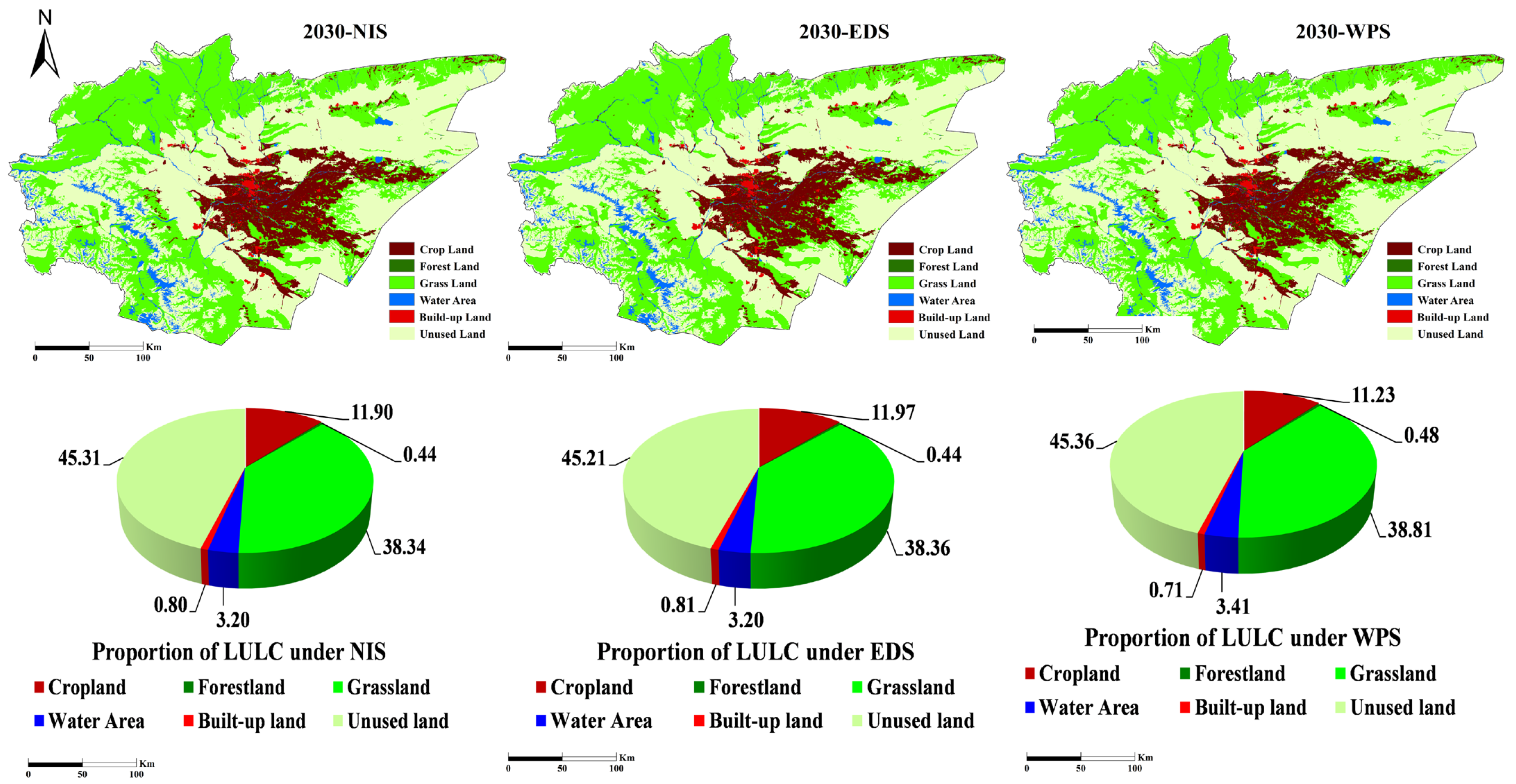
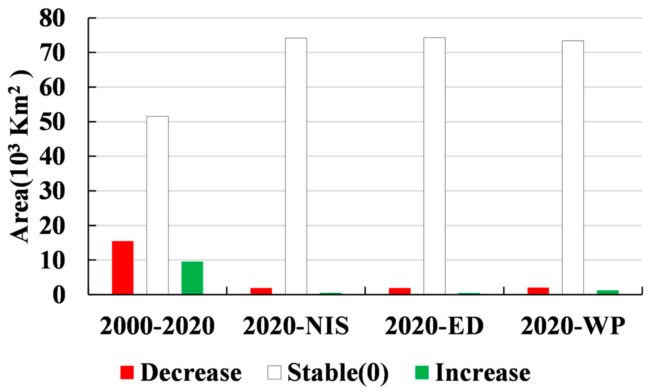
3.1.2. Spatiotemporal Characteristics of Land-Use Change from 2000 to 2030

As can be seen from the historical data, the proportion of each LULC type in the KRB remains relatively stable, which indicates that the LULC trend in this region will likely not undergo drastic structural changes in the future (Figure 5). From 2000 to 2020, the overall changing trends were increases in cropland, built-up land, and unused land and decreases in grassland, forestland, and water areas. Among these changes, water areas had the greatest decrement, with a rate of change of 56.06%, while cropland and built-up land further expanded by 2446 km2 and 343 km2 from 2000 to 2010, respectively. Grassland mainly intermingled with water areas in the basin’s northern and western mountainous regions, decreasing by 2532 km2 from 2000 to 2020, for a rate of change of 7.64%.
The PLUS model was applied in this paper to predict the spatial distribution of land- use demand for 2030 under various scenarios (Figure 6). Under the natural increase scenario, the largest decrement occurred in grassland, which decreased by 4.01% (1226.03 km2), while unused land increased the most, expanding by 998 km2. The changes in forestland were the reverse of the previous trend, increasing by 4.13%. Under the economic development scenario (Figure 6), built-up land and cropland saw a rapid expansion in area of 24.65% and 16.49%, respectively. The area of water bodies likewise grew rapidly, with the water protection scenario predicting a 25.32% increase. However, while the areas of built-up land, cropland, and unused land all showed an increasing trend under the WPS, the growth rate was significantly lower than that under the NIS and EDS.

3.2. Changes in Habitat Quality

3.2.1. Changes in HQ during 2000–2020

Table 4 presents spatial variation statistics of HQ for different periods in the KRB. As shown, there was a gradual decrease in HQ, with average values of 0.54, 0.50, and 0.49 in 2000, 2010, and 2020, respectively.
This paper divides HQ into five grades at equal intervals of 0.2. The grades are as follows: very poor (0–0.2), poor (0.2–0.4), moderate (0.4–0.6), good (0.6–0.8), and excellent (0.8–1). Our statistical analysis shows that HQ in the KRB was dominated by poor grades (Figure 7), which accounted for about 40% to 45% of the total area. During 2000–2020, the proportion of good and excellent grades decreased from 43.2% and 7.69% in 2000 to 39.93% and 3.79% in 2020. The distribution of these two grades was concentrated in the mountainous areas in the northern part of the KRB and the periphery of the oasis.
Meanwhile, there was a significant increase in very poor and poor grade areas, rising by 1.04% and 2.98%, respectively. This increase mainly occurred in unused lands, such as Gobi sandy land, and salinized land. At the same time, moderate-grade areas in the oasis increased from 6.26% in 2000 to 9.45% in 2020. The main LULC type included in the expansion was cropland.

3.2.2. Future Changes in HQ under Different Scenarios

For mean HQ values, the EDS shows the largest decrease from 2020 to 2030 (Table 4), with a decline of 18.74%. Figure 8 illustrates the change in the KRB’s HQ from 2000 to 2030. The smallest decrease occurred under the WPS, with a drop of 11.89%. This suggests that HQ in the study area is predicted to decrease more significantly under the NIS and EDS than under the WPS. Thus, implementing ecological protection measures under the social economy would be beneficial for improving HQ (Figure 7).
The NIS exhibited a continuous deterioration in HQ, with a decrease in area of 1889 km2 (Figure 8). The decrease mainly occurred at the edge of the oasis and in unused land. In contrast, under the EDS, moderate-grade area changed significantly, increasing by 8.08%, although the overall improvement area under this scenario was only about 455 km2, which is quite small. The WPS shows the largest improvement with an area expansion of 1238 km2, mainly due to the increase in area graded as excellent (Figure 8).

3.3. Changes in Carbon Storage

3.3.1. Changes in CS during 2000–2020

Carbon storage in the KRB during the historical period was estimated using the InVEST model. As shown in Table 5, CS experienced a fluctuating upward trend that increased from 49.19 × 10⁶ t in 2000 to 49.73 × 10⁶ t in 2010 and then decreased to 49.26 × 10⁶ t in 2020. During 2000–2020, total CS increased by 0.07 × 10⁶ t. Gains in CS occurred in cultivated land, with an increase of 2.32 × 10⁶ t, while losses in CS occurred in grassland, forestland, and water area, for a total loss of 2.79 × 10⁶ t. Spatially, the distribution of CS in the KRB remained basically stable and without drastic migration or other changes. From 2000 to 2020, decreases in CS in the KRB mainly occurred in mountainous areas and oases in the plain regions, while increases in CS occurred in the southwest (Figure 9a).

3.3.2. Future Changes in CS under Different Scenarios

Total CS under the three test scenarios in 2030 showed a downward trend (Table 5). During 2020–2030, the decrease in CS was smaller under the NIS (0.77 × 10⁶ t) compared to the EDS (0.79 × 10⁶ t). However, the WPS resulted in the largest loss of CS, with a total reduction of −1.08 × 10⁶ t in 2020–2030 occurring mainly in the plains area. Combined with LULC changes in the study area, we found that the WPS had the largest loss of CS due to grassland conversion (1.42 × 10⁶ t), while the increase in CS due to the expansion of cropland was smaller (only around 0.34 × 10⁶ t) than in the EDS and NIS (Figure 9b).

3.4. Key LULC Identifications and Influences of Land-Use Changes on ESs

Figure 10 shows the contribution of different land-use changes to ESs. From 2000 to 2020, the conversion of forestland, grassland, and built-up land had a negative impact on HQ. However, under the three future scenarios, the most significant negative impact on HQ comes from the conversion of grassland. The order of HQCI from largest to smallest in the three scenarios is EDS > NIS > WPS. Conversely, the conversion of unused land into cropland has a more positive impact on HQ, with the most significant positive impact expected under the EDS (HQCI = 11.74).
Additionally, grassland conversion had a significant impact on CS in the KRB. As can be seen in Figure 10, the conversion of unused land to grassland had the greatest positive impact (CSCI = 19.60). However, the conversion of grassland to other types of land use (except for forestland) had a significant negative impact on CS, especially the conversion of grassland to unused land (CSCI = −21.91). Under the three future scenarios, the negative impact on CS of the conversion of grassland to unused land is most significant under the EDS (CSCI = −26.25), while the negative impact is least under the WPS (CSCI = −21.26). Moreover, the conversion of forestland and grassland to cropland, built-up land, and unused land had different negative effects on CS. It is worth noting that the positive effect of the conversion to forestland on CS grows more significantly in the future scenario. To sum up, the expansion of cropland, built-up land, and unused land had a negative impact on ESs, which was more significant on CS, while the conversion to grassland and forestland had a significant positive impact on ESs.

4. Discussion

4.1. Changes in HQ and CS under Different LULCs

The KRB, which is one of the most significant headwaters of the TRB, has a very delicate ecological environment [61]. Currently, the economic and social development in the region mainly relies on traditional agriculture and animal husbandry. Due to extensive irrigation using unsophisticated techniques, however, the need for irrigation water has grown steadily over time [62]. The utilization efficiency of agricultural irrigation water in the KRB is considerably lower than both the average in Xinjiang and all across China. Moreover, the region has also witnessed a surge in population and economic development over the past two decades, with the GDP jumping from 42.90 × 10⁸ yuan in 2000 to 645.85 × 10⁸ yuan in 2020.
The result of these rapid changes has been a significant increase in cropland and built-up land [57], with cropland alone expanding 55.76% (Figure 5), mainly in the lower basin. However, at the same time, significant reductions have been observed in forestland, grassland, and water areas in the KRB. Forestland declined the most during 2010–2020, with a decreasing rate of −24.55%. Similarly, grassland and water areas decreased at a changing rate of 7.64%, and 56.06%, respectively (Figure 6). Accordingly, the ecosystem services of the KRB showed a corresponding increase in degradation in 2000–2020 (Figure 7 and Figure 8). This finding is in line with results presented in other studies of similar arid regions [47,63].
Meanwhile, the spatial distribution of ESs exhibited a decreasing trend from north to south and from east to west, with the lowest values found in the middle of the study area. This occurred because the ESs were affected by factors, such as land-use patterns, human activities, and climate change [64]. Of all the land types studied in this paper, forestland and grassland provide the highest value of ESs [65], as they are rich in biodiversity and have a high capacity for carbon sequestration and runoff regulation. In contrast, cropland, built-up areas, and unused land provide much lower services [66]. Desertification affects biological and geochemical processes, which in turn puts soil at risk and reduces its carbon content [67]. Deforested land that has been abandoned due to a lack of water or soil fertility is often blindly reclaimed, resulting in a vicious cycle that not only destroys the vegetation, causing the forest to retreat into the sand, but also loosens the surface, promoting the formation of new sand sources.
In addition, climate change affects hydrological processes and the distribution of water and energy [68]. The results of the spatial distribution of HQ and CS in this paper show that the areas characterized by high ES values in the KRB are distributed mostly in forestland and grassland at higher elevations [8,30]. In the context of climate warming, the melting of snow and ice in mountain areas provides sufficient water resources for the study region, reduces water stress on plants, and enhances the production of NPP and gas control, thereby increasing carbon sequestration. Although melting snow and ice increase surface runoff, the continued expansion of cropland is causing a surge in agricultural water use, intensifying the fragmentation of ecological land in the region and gradually degrading downstream vegetation without water [69]. The result is a reduction in ESs that threatens the overall stability of the ecosystem.
This study further predicts the impact of future land-use changes on ecosystem services. The changes in LULC and ESs in 2020–2030 (Figure 5, Figure 7, Figure 8 and Figure 9) are similar to those in the past. In addition, the results of ESCI confirm that the conversion of grassland to unused land had the greatest negative impact on ESs [30,70] and that the impact was most significant under the economic development scenario (Figure 10). In contrast, the conversion of other lands to forestland had a greater positive impact on ESs, with the positive impact being most significant under the water protection scenario [71].
Therefore, in order to protect the ecological environment of the KRB, land conversion management should be strengthened to reduce the conversion of land with high ES value to land with low ES value. Special attention should be paid to the rational development of water resources in the process of agricultural and urbanization development to improve the efficiency of water resource use, while ecological engineering should be strengthened to prevent ecological degradation caused by overexploitation.

4.2. Advantages of the Model Used in This Study

The InVEST model used in this study has been widely employed in the field of ecosystem services studies [15,25], due to its unique advantages in spatial representation [23]. Researchers have discovered that the model is also applicable to arid regions [15]. For example, Wang, Li, Mao, Li, Wang, and Lin [24] used the INVEST model to assess CS based on climate change scenarios in the city of Bortala, Xinjiang. They found that the simulation results of the model were close to the actual situation. Moreover, in a comparison with other models, such as the CA-Markov, CLUE-S, and FLUS, the PLUS model used in the current study is suitable for large-scale land-use simulations, as it gives higher simulation accuracy. This result is similar to the results presented in other studies applying PLUS, such as [34,56,72]. The PLUS-InVEST model has integrated a new land-use expansion strategy and growth mechanism to accurately simulate the changes in different types of land-use patches with high accuracy [47].

4.3. Limitations and Uncertainties

Combining the PLUS and InVEST models, the spatiotemporal variations of two types of ESs from 2000 to 2030 in the KRB were analyzed in this paper. However, there are some shortcomings that need to be addressed and improved upon in future investigations.
Firstly, the InVEST model calculates the habitat quality based on the weights of the selected threat factors and the sensitivity data. However, the weights and sensitivity data of the threat factors in this paper were obtained by referring to the relevant literature, and the classification of LULC was a first-level classification that included only six land-use categories. All of these uncertainties may have an impact on the assessment of HQ. Thus, LULC data with higher resolution and finer land classification should be obtained for future research to improve the weights and sensitivity data of threat factors and make the assessment results more reliable.
Secondly, due to the lack of measured data, the carbon density data used for land use in this paper were also obtained from relevant published research, and the data do not change over time. Therefore, combining a large amount of measured data to improve the simulation accuracy of the model is vital in future research.
In addition, this study only focused on the spatiotemporal changes in two kinds of ecosystem services, namely habitat quality and carbon storage. Future research should encompass a broader range of factors, such as the water yield, soil conservation, and food production, to provide a more comprehensive assessment of ESs. Furthermore, because changes in ES can be influenced by a combination of several factors, such as climate change, topographic factors, and socioeconomic factors, along with policy factors at the national and local levels, the synergistic effects of these factors on ES should be considered. Adopting such an approach would provide a reliable scientific basis for the coordinated development of ecology, land use, and the economy in arid regions.

5. Conclusions

This study focused on the Kaxghar River Basin (KRB) in Xinjiang, China, and aimed to investigate the spatiotemporal distribution and changing patterns of ecosystem services (ESs) in the region, including habitat quality (HQ) and carbon storage (CS), using an integrated PLUS-InVEST model. The main conclusions are as follows:
(1) The PLUS model has higher simulation accuracy and is suitable for land-use simulations in the study area. Of the land-use types reviewed in this paper, cropland, grassland, and water bodies were identified as undergoing the most significant changes from 2000 to 2030. The economic development scenario (EDS) showed the highest growth rate of cropland and built-up land, with an area increase of 1196.69 km2 and 120.70 km2, respectively. The water protection scenario (WPS) led to a 25.32% increase in the water body area, indicating the effectiveness of the WPS in preserving water resources.
(2) Over the past two decades, habitat quality in the KRB has remained at a relatively moderate level. Under the EDS scenario, the area with low-grade HQ increased at the fastest rate, while high-HQ-grade areas decreased the most. Meanwhile, under the WPS scenario, 1238 km2 of land area saw an increase in HQ, indicating that implementing ecological protection measures can be beneficial for improving habitat quality.
(3) The total CS in the KRB fluctuated upwards over the study period, with the most significant changes observed from 2010 to 2020. However, under the three different scenarios, the total CS showed a decreasing trend, with the smallest decrease observed under the NIS. High-carbon-storage areas were mainly distributed in regions with a complex terrain and sparse population, while low-carbon-storage areas were scattered throughout the study area.
(4) Different LULC changes had varying impacts on the ESs. The ESCI index results showed that the conversion of grassland to unused land had the greatest negative impact on both HQ and CS, especially under the EDS. In contrast, the conversion of other land to forestland had a more positive impact on HQ and CS, with the most significant positive impact observed under the WPS.

Author Contributions

Z.K. and Y.C. conceived the original design of this paper; Y.L. and C.W. put forward valuable suggestions for this article. All authors have read and agreed to the published version of the manuscript.

Funding

The research was supported by the Third Xinjiang Scientific Expedition Program (Grant No. 2022xjkk0106).

Data Availability Statement

The data presented in this study are available on request from the corresponding author.

Conflicts of Interest

The authors declare no conflict of interest.

References

  1. Costanza, R.; Groot, R.D.; Braat, L.; Kubiszewski, I.; Fioramonti, L.; Sutton, P.; Farber, S.; Grasso, M. Twenty years of ecosystem services: How far have we come and how far do we still need to go? Ecosyst. Serv. 2017, 28, 1–16. [Google Scholar] [CrossRef]
  2. Mehring, M.; Ott, E.; Hummel, D. Ecosystem services supply and demand assessment: Why social-ecological dynamics matter. Ecosyst. Serv. 2018, 30, 124–125. [Google Scholar] [CrossRef]
  3. Yin, L.T.; Zheng, W.; Shi, H.H.; Ding, D.W. Ecosystem services assessment and sensitivity analysis based on ANN model and spatial data: A case study in Miaodao Archipelago. Ecol. Indic. 2022, 135, 108511. [Google Scholar] [CrossRef]
  4. Millennium Ecosystem Assessment. Ecosystems and Human Well-Being: Current State and Trends; Island Press: Washington, DC, USA, 2005; Volume 5. [Google Scholar]
  5. Ye, Y.Q.; Bryan, B.A.; Zhang, J.E.; Connor, J.D.; Chen, L.L.; Qin, Z.; He, M.Q. Changes in land-use and ecosystem services in the Guangzhou-Foshan Metropolitan Area, China from 1990 to 2010: Implications for sustainability under rapid urbanization. Ecol. Indic. 2018, 93, 930–941. [Google Scholar] [CrossRef]
  6. Xue, C.L.; Zhang, H.Q.; Wu, S.M.; Chen, J.P.; Chen, X.H. Spatial-temporal evolution of ecosystem services and its potential drivers: A geospatial perspective from Bairin Left Banner, China. Ecol. Indic. 2022, 137, 108760. [Google Scholar] [CrossRef]
  7. Costanza, R.; d’Arge, R.; De Groot, R.; Farber, S.; Grasso, M.; Hannon, B.; Limburg, K.; Naeem, S.; O’Neill, R.V.; Paruelo, J. The value of the world’s ecosystem services and natural capital. Nature 1997, 387, 253–260. [Google Scholar] [CrossRef]
  8. Fang, Z.; Ding, T.H.; Chen, J.Y.; Xue, S.; Zhou, Q.; Wang, Y.D.; Wang, Y.X.; Huang, Z.D.; Yang, S.L. Impacts of land use/land cover changes on ecosystem services in ecologically fragile regions. Sci. Total Environ. 2022, 831, 154967. [Google Scholar] [CrossRef]
  9. Lyu, R.F.; Clarke, K.C.; Zhang, J.M.; Feng, J.L.; Jia, X.H.; Li, J.J. Dynamics of spatial relationships among ecosystem services and their determinants: Implications for land use system reform in Northwestern China. Land Use Policy 2021, 102, 105231. [Google Scholar] [CrossRef]
  10. Sannigrahi, S.; Zhang, Q.; Joshi, P.K.; Sutton, P.C.; Keesstra, S.; Roy, P.S.; Pilla, F.; Basu, B.; Wang, Y.; Jha, S.; et al. Examining effects of climate change and land use dynamic on biophysical and economic values of ecosystem services of a natural reserve region. J. Clean. Prod. 2020, 257, 120424. [Google Scholar] [CrossRef]
  11. Huang, A.; Xu, Y.; Sun, P.; Zhou, G.; Liu, C.; Lu, L.; Xiang, Y.; Wang, H. Land use/land cover changes and its impact on ecosystem services in ecologically fragile zone: A case study of Zhangjiakou City, Hebei Province, China. Ecol. Indic. 2019, 104, 604–614. [Google Scholar] [CrossRef]
  12. Qi, X.; Li, Q.; Yue, Y.; Liao, C.; Zhai, L.; Zhang, X.; Wang, K.; Zhang, C.; Zhang, M.; Xiong, Y. Rural–Urban Migration and Conservation Drive the Ecosystem Services Improvement in China Karst: A Case Study of HuanJiang County, Guangxi. Remote Sens. 2021, 13, 566. [Google Scholar] [CrossRef]
  13. Benra, F.; De Frutos, A.; Gaglio, M.; Alvarez-Garreton, C.; Felipe-Lucia, M.; Bonn, A. Mapping water ecosystem services: Evaluating InVEST model predictions in data scarce regions. Environ. Model. Softw. 2021, 138, 104982. [Google Scholar] [CrossRef]
  14. Dong, X.B.; Wang, X.W.; Wei, H.J.; Fu, B.J.; Wang, J.J.; Uriarte-Ruiz, M. Trade-offs between local farmers’ demand for ecosystem services and ecological restoration of the Loess Plateau, China. Ecosyst. Serv. 2021, 49, 101295. [Google Scholar] [CrossRef]
  15. Daneshi, A.; Brouwer, R.; Najafinejad, A.; Panahi, M.; Zarandian, A.; Maghsood, F.F. Modelling the impacts of climate and land use change on water security in a semi-arid forested watershed using InVEST. J. Hydrol. 2021, 593, 125621. [Google Scholar] [CrossRef]
  16. Bai, Y.; Chen, Y.; Alatalod, J.M.; Yang, Z.; Jiang, B. Scale effects on the relationships between land characteristics and ecosystem services- a case study in Taihu Lake Basin, China. Sci. Total Environ. 2020, 716, 137083. [Google Scholar] [CrossRef]
  17. Chen, J.Y.; Jiang, B.; Bai, Y.; Xu, X.B.; Alatalo, J.M. Quantifying ecosystem services supply and demand shortfalls and mismatches for management optimisation. Sci. Total Environ. 2019, 650, 1426–1439. [Google Scholar] [CrossRef]
  18. Zheng, D.; Wang, Y.; Hao, S.; Xu, W.; Lv, L.; Yu, S. Spatial-temporal variation and tradeoffs/synergies analysis on multiple ecosystem services: A case study in the Three-River Headwaters region of China. Ecol. Indic. 2020, 116, 106494. [Google Scholar] [CrossRef]
  19. Wu, Y.; Tao, Y.; Yang, G.S.; Ou, W.X.; Pueppke, S.; Sun, X.; Chen, G.T.; Tao, Q. Impact of land use change on multiple ecosystem services in the rapidly urbanizing Kunshan City of China: Past trajectories and future projections. Land Use Policy 2019, 85, 419–427. [Google Scholar] [CrossRef]
  20. Wang, X.Z.; Wu, J.Z.; Liu, Y.L.; Hai, X.Y.; Shanguan, Z.P.; Deng, L. Driving factors of ecosystem services and their spatiotemporal change assessment based on land use types in the Loess Plateau. J. Environ. Manag. 2022, 311, 114835. [Google Scholar] [CrossRef]
  21. Ma, S.; Wang, L.-J.; Zhu, D.; Zhang, J. Spatiotemporal changes in ecosystem services in the conservation priorities of the southern hill and mountain belt, China. Ecol. Indic. 2021, 122, 107225. [Google Scholar] [CrossRef]
  22. Li, X.; Yu, X.; Wu, K.; Feng, Z.; Liu, Y.; Li, X. Land-use zoning management to protecting the Regional Key Ecosystem Services: A case study in the city belt along the Chaobai River, China. Sci. Total Environ. 2021, 762, 143167. [Google Scholar] [CrossRef] [PubMed]
  23. Yang, S.L.; Bai, Y.; Alatalo, J.M.; Wang, H.M.; Jiang, B.; Liu, G.; Chen, J.Y. Spatio-temporal changes in water-related ecosystem services provision and trade-offs with food production. J. Clean. Prod. 2021, 286, 125316. [Google Scholar] [CrossRef]
  24. Wang, Z.; Li, X.; Mao, Y.; Li, L.; Wang, X.; Lin, Q. Dynamic simulation of land use change and assessment of carbon storage based on climate change scenarios at the city level: A case study of Bortala, China. Ecol. Indic. 2022, 134, 108499. [Google Scholar] [CrossRef]
  25. Jia, G.; Hu, W.; Zhang, B.; Li, G.; Shen, S.; Gao, Z.; Li, Y. Assessing impacts of the Ecological Retreat project on water conservation in the Yellow River Basin. Sci. Total Environ. 2022, 828, 154483. [Google Scholar] [CrossRef]
  26. Tang, F.; Fu, M.; Wang, L.; Song, W.; Yu, J.; Wu, Y. Dynamic evolution and scenario simulation of habitat quality under the impact of land-use change in the Huaihe River Economic Belt, China. PLoS ONE 2021, 16, e0249566. [Google Scholar] [CrossRef]
  27. Chen, T.Q.; Feng, Z.; Zhao, H.F.; Wu, K.N. Identification of ecosystem service bundles and driving factors in Beijing and its surrounding areas. Sci. Total Environ. 2020, 711, 134687. [Google Scholar] [CrossRef]
  28. Gomes, E.; Inácio, M.; Bogdzevič, K.; Kalinauskas, M.; Karnauskaitė, D.; Pereira, P. Future scenarios impact on land use change and habitat quality in Lithuania. Environ. Res. 2021, 197, 111101. [Google Scholar] [CrossRef]
  29. Li, J.; Zhang, C.; Zhu, S. Relative contributions of climate and land-use change to ecosystem services in arid inland basins. J. Clean. Prod. 2021, 298, 126844. [Google Scholar] [CrossRef]
  30. Li, J.; Dong, S.; Li, Y.; Wang, Y.; Li, Z.; Li, F. Effects of land use change on ecosystem services in the China–Mongolia–Russia economic corridor. J. Clean. Prod. 2022, 360, 132175. [Google Scholar] [CrossRef]
  31. Xing, L.; Hu, M.; Wang, Y. Integrating ecosystem services value and uncertainty into regional ecological risk assessment: A case study of Hubei Province, Central China. Sci. Total Environ. 2020, 740, 140126. [Google Scholar] [CrossRef]
  32. Wang, H.; Hu, Y.; Yan, H.; Liang, Y.; Guo, X.; Ye, J. Trade-off among grain production, animal husbandry production, and habitat quality based on future scenario simulations in Xilinhot. Sci. Total Environ. 2022, 817, 153015. [Google Scholar] [CrossRef]
  33. Peng, K.; Jiang, W.; Ling, Z.; Hou, P.; Deng, Y. Evaluating the potential impacts of land use changes on ecosystem service value under multiple scenarios in support of SDG reporting: A case study of the Wuhan urban agglomeration. J. Clean. Prod. 2021, 307, 127321. [Google Scholar] [CrossRef]
  34. Liang, X.; Guan, Q.; Clarke, K.C.; Liu, S.; Wang, B.; Yao, Y. Understanding the drivers of sustainable land expansion using a patch-generating land use simulation (PLUS) model: A case study in Wuhan, China. Comput. Environ. Urban Syst. 2021, 85, 101569. [Google Scholar] [CrossRef]
  35. Liu, X.; Liu, Y.; Wang, Y.; Liu, Z. Evaluating potential impacts of land use changes on water supply–demand under multiple development scenarios in dryland region. J. Hydrol. 2022, 610, 127811. [Google Scholar] [CrossRef]
  36. Wang, J.; Zhang, J.; Xiong, N.; Liang, B.; Wang, Z.; Cressey, E.L. Spatial and Temporal Variation, Simulation and Prediction of Land Use in Ecological Conservation Area of Western Beijing. Remote Sens. 2022, 14, 1452. [Google Scholar] [CrossRef]
  37. Ferreira, M.R.; Almeida, A.M.; Quintela-Sabarís, C.; Roque, N.; Fernandez, P.; Ribeiro, M.M. The role of littoral cliffs in the niche delimitation on a microendemic plant facing climate change. PLoS ONE 2021, 16, e0258976. [Google Scholar] [CrossRef]
  38. Wang, F.; Chen, Y.N.; Li, Z.; Fang, G.H.; Li, Y.P.; Xia, Z.H. Assessment of the Irrigation Water Requirement and Water Supply Risk in the Tarim River Basin, Northwest China. Sustainability 2019, 11, 4941. [Google Scholar] [CrossRef]
  39. Wang, W.; Chen, Y.; Wang, W.; Jiang, J.; Cai, M.; Xu, Y. Evolution characteristics of groundwater and its response to climate and land-cover changes in the oasis of dried-up river in Tarim Basin. J. Hydrol. 2021, 594, 125644. [Google Scholar] [CrossRef]
  40. Zhang, Z.; Xia, F.; Yang, D.; Huo, J.; Wang, G.; Chen, H. Spatiotemporal characteristics in ecosystem service value and its interaction with human activities in Xinjiang, China. Ecol. Indic. 2020, 110, 105826. [Google Scholar] [CrossRef]
  41. Maimaiti, B.; Chen, S.; Kasimu, A.; Mamat, A.; Aierken, N.; Chen, Q. Coupling and Coordination Relationships between Urban Expansion and Ecosystem Service Value in Kashgar City. Remote Sens. 2022, 14, 2557. [Google Scholar] [CrossRef]
  42. Zheng, W.; Li, S.; Ke, X.; Li, X.; Zhang, B. The impacts of cropland balance policy on habitat quality in China: A multiscale administrative perspective. J. Environ. Manag. 2022, 323, 116182. [Google Scholar] [CrossRef] [PubMed]
  43. Lei, J.; Chen, Y.; Li, L.; Chen, Z.; Chen, X.; Wu, T.; Li, Y. Spatiotemporal change of habitat quality in Hainan Island of China based on changes in land use. Ecol. Indic. 2022, 145, 109707. [Google Scholar] [CrossRef]
  44. Wu, J.; Luo, J.; Zhang, H.; Qin, S.; Yu, M. Projections of land use change and habitat quality assessment by coupling climate change and development patterns. Sci. Total Environ. 2022, 847, 157491. [Google Scholar] [CrossRef] [PubMed]
  45. Tang, F.; Wang, L.; Guo, Y.; Fu, M.; Huang, N.; Duan, W.; Luo, M.; Zhang, J.; Li, W.; Song, W. Spatio-temporal variation and coupling coordination relationship between urbanisation and habitat quality in the Grand Canal, China. Land Use Policy 2022, 117, 106119. [Google Scholar] [CrossRef]
  46. Chen, X.; Yu, L.; Cao, Y.; Xu, Y.; Zhao, Z.; Zhuang, Y.; Liu, X.; Du, Z.; Liu, T.; Yang, B.; et al. Habitat quality dynamics in China’s first group of national parks in recent four decades: Evidence from land use and land cover changes. J. Environ. Manag. 2023, 325, 116505. [Google Scholar] [CrossRef]
  47. Wei, Q.; Abudureheman, M.; Halike, A.; Yao, K.; Yao, L.; Tang, H.; Tuheti, B. Temporal and spatial variation analysis of habitat quality on the PLUS-InVEST model for Ebinur Lake Basin, China. Ecol. Indic. 2022, 145, 109632. [Google Scholar] [CrossRef]
  48. Wei, L.; Zhou, L.; Sun, D.; Yuan, B.; Hu, F. Evaluating the impact of urban expansion on the habitat quality and constructing ecological security patterns: A case study of Jiziwan in the Yellow River Basin, China. Ecol. Indic. 2022, 145, 109544. [Google Scholar] [CrossRef]
  49. Leh, M.D.K.; Matlock, M.D.; Cummings, E.C.; Nalley, L.L. Quantifying and mapping multiple ecosystem services change in West Africa. Agric. Ecosyst. Environ. 2013, 165, 6–18. [Google Scholar] [CrossRef]
  50. Wu, L.; Sun, C.; Fan, F. Estimating the characteristic spatiotemporal variation in habitat quality using the invest model—A case study from Guangdong–Hong Kong–Macao Greater Bay Area. Remote Sens. 2021, 13, 1008. [Google Scholar] [CrossRef]
  51. Zhu, C.; Zhang, X.; Zhou, M.; He, S.; Gan, M.; Yang, L.; Wang, K. Impacts of urbanization and landscape pattern on habitat quality using OLS and GWR models in Hangzhou, China. Ecol. Indic. 2020, 117, 106654. [Google Scholar] [CrossRef]
  52. Gao, R.; Chuai, X.; Ge, J.; Wen, J.; Zhao, R.; Zuo, T. An integrated tele-coupling analysis for requisition–compensation balance and its influence on carbon storage in China. Land Use Policy 2022, 116, 106057. [Google Scholar] [CrossRef]
  53. Zhou, J.; Zhao, Y.; Huang, P.; Zhao, X.; Feng, W.; Li, Q.; Xue, D.; Dou, J.; Shi, W.; Wei, W.J.E.I. Impacts of ecological restoration projects on the ecosystem carbon storage of inland river basin in arid area, China. Ecol. Indic. 2020, 118, 106803. [Google Scholar] [CrossRef]
  54. Nie, X.; Lu, B.; Chen, Z.; Yang, Y.; Chen, S.; Chen, Z.; Wang, H. Increase or decrease? Integrating the CLUMondo and InVEST models to assess the impact of the implementation of the Major Function Oriented Zone planning on carbon storage. Ecol. Indic. 2020, 118, 106708. [Google Scholar] [CrossRef]
  55. Zhu, G.; Qiu, D.; Zhang, Z.; Sang, L.; Liu, Y.; Wang, L.; Zhao, K.; Ma, H.; Xu, Y.; Wan, Q. Land-use changes lead to a decrease in carbon storage in arid region, China. Ecol. Indic. 2021, 127, 107770. [Google Scholar] [CrossRef]
  56. Zhang, S.; Yang, P.; Xia, J.; Wang, W.; Cai, W.; Chen, N.; Hu, S.; Luo, X.; Li, J.; Zhan, C. Land use/land cover prediction and analysis of the middle reaches of the Yangtze River under different scenarios. Sci. Total Environ. 2022, 833, 155238. [Google Scholar] [CrossRef]
  57. Xie, L.; Wang, H.; Liu, S. The ecosystem service values simulation and driving force analysis based on land use/land cover: A case study in inland rivers in arid areas of the Aksu River Basin, China. Ecol. Indic. 2022, 138, 108828. [Google Scholar] [CrossRef]
  58. Zhang, S.; Zhong, Q.; Cheng, D.; Xu, C.; Chang, Y.; Lin, Y.; Li, B. Landscape ecological risk projection based on the PLUS model under the localized shared socioeconomic pathways in the Fujian Delta region. Ecol. Indic. 2022, 136, 108642. [Google Scholar] [CrossRef]
  59. Zhang, Y.; Li, Y.; Lv, J.; Wang, J.; Wu, Y. Scenario simulation of ecological risk based on land use/cover change—A case study of the Jinghe county, China. Ecol. Indic. 2021, 131, 108176. [Google Scholar] [CrossRef]
  60. Yang, Y. Evolution of habitat quality and association with land-use changes in mountainous areas: A case study of the Taihang Mountains in Hebei Province, China. Ecol. Indic. 2021, 129, 107967. [Google Scholar] [CrossRef]
  61. Li, J.; Lei, J.; Li, S.; Yang, Z.; Tong, Y.; Zhang, S.; Duan, Z. Spatiotemporal analysis of the relationship between urbanization and the eco-environment in the Kashgar metropolitan area, China. Ecol. Indic. 2022, 135, 108524. [Google Scholar] [CrossRef]
  62. Fang, G.; Chen, Y.; Li, Z. Variation in agricultural water demand and its attributions in the arid Tarim River Basin. J. Agric. Sci. 2018, 156, 301–311. [Google Scholar] [CrossRef]
  63. Li, S.; Liu, Y.; Yang, H.; Yu, X.; Zhang, Y.; Wang, C. Integrating ecosystem services modeling into effectiveness assessment of national protected areas in a typical arid region in China. J. Environ. Manag. 2021, 297, 113408. [Google Scholar] [CrossRef] [PubMed]
  64. Fang, J.; Song, H.; Zhang, Y.; Li, Y.; Liu, J. Climate-dependence of ecosystem services in a nature reserve in northern China. PLoS ONE 2018, 13, e0192727. [Google Scholar] [CrossRef] [PubMed]
  65. Ocampo, M.C.E.; Castillo Santiago, M.Á.; Ochoa-Gaona, S.; Enríquez, P.L.; Sibelet, N. Assessment of habitat quality and landscape connectivity for forest-dependent cracids in the Sierra Madre del Sur Mesoamerican biological corridor, Mexico. Trop. Conserv. Sci. 2019, 12, 1940082919878827. [Google Scholar] [CrossRef]
  66. Pan, N.H.; Guan, Q.Y.; Wang, Q.Z.; Sun, Y.F.; Li, H.C.; Ma, Y.R. Spatial Differentiation and Driving Mechanisms in Ecosystem Service Value of Arid Region: A case study in the middle and lower reaches of Shule River Basin, NW China. J. Clean. Prod. 2021, 319, 128718. [Google Scholar] [CrossRef]
  67. Darbalaeva, D.; Mikheeva, A.; Sanzheev, E.; Zhamyanov, D.; Osodoev, P.; Batomunkuev, V. Ecosystem Service’ Assessment of the Desertification Areas of Mongolia. Earth Syst. Environ. 2022, 1–14. [Google Scholar] [CrossRef]
  68. Deng, H.; Chen, Y.; Li, Q.; Lin, G. Loss of terrestrial water storage in the Tianshan mountains from 2003 to 2015. Int. J. Remote Sens. 2019, 40, 8342–8358. [Google Scholar] [CrossRef]
  69. Zhou, H.; Chen, Y.; Zhu, C.; Li, Z.; Fang, G.; Li, Y.; Fu, A. Climate change may accelerate the decline of desert riparian forest in the lower Tarim River, Northwestern China: Evidence from tree-rings of Populus euphratica. Ecol. Indic. 2020, 111, 105997. [Google Scholar] [CrossRef]
  70. Zhang, X.; Song, W.; Lang, Y.; Feng, X.; Yuan, Q.; Wang, J. Land use changes in the coastal zone of China’s Hebei Province and the corresponding impacts on habitat quality. Land Use Policy 2020, 99, 104957. [Google Scholar] [CrossRef]
  71. Zhang, T.; Chen, Y. The effects of landscape change on habitat quality in arid desert areas based on future scenarios: Tarim River Basin as a case study. Front. Plant Sci. 2022, 13, 1031859. [Google Scholar] [CrossRef]
  72. Li, C.; Wu, Y.M.; Gao, B.P.; Zheng, K.J.; Wu, Y.; Li, C. Multi-scenario simulation of ecosystem service value for optimization of land use in the Sichuan-Yunnan ecological barrier, China. Ecol. Indic. 2021, 132, 108328. [Google Scholar] [CrossRef]
Figure 1. Location of the study area. (The map is based on the standard map number GS (2016) 1666 downloaded from the standard map service website of the National Bureau of Mapping Geographic Information, and the base map is not modified).
Remotesensing 15 02476 g001
Figure 2. Driving factors affecting the spatial distribution of LULC.
Remotesensing 15 02476 g002
Figure 3. Analysis framework of the research.
Remotesensing 15 02476 g003
Figure 4. Observed (2000, 2010, 2020) data and simulation (2010a, 2020a) results for LULC in the KRB.
Remotesensing 15 02476 g004
Figure 5. LULC area changes during 2000–2030.
Remotesensing 15 02476 g005
Figure 6. Spatial distribution and proportion of LULC from 2020 to 2030 under the three test scenarios.
Remotesensing 15 02476 g006
Figure 7. Spatial distribution of HQ in KRB during 2000–2030.
Remotesensing 15 02476 g007
Figure 8. Changes of HQ in the KRB during 2000–2030.
Remotesensing 15 02476 g008
Figure 9. Spatial distribution and changes in CS in the KRB during 2000–2020 and 2020–2030 under the three test scenarios.
Remotesensing 15 02476 g009
Figure 10. Contribution of land-use conversion to changes in ESs (2000–2030).
Remotesensing 15 02476 g010
Table 1. Threat factors and sensitivity of each land-use type.
Habitat SuitabilitySensitivity to Threats
CroplandBuilt-Up LandUnused Land
Decline type LinearExponentialLinear
Maximum threat distance0.3586
Weight0.60.40.5
Cropland0.500.90.5
Forestland10.60.80.2
Grassland0.90.80.50.3
Water area10.50.40.5
Built-up land0000
Unused land0.10.20.60
Table 2. Carbon density data for each land-use type in the study area (kg/m2).
Land Use TypesAbove-GroundBelow-GroundSoil Organics
Cropland0.11.457.95
Forestland0.762.0815.88
Grassland0.631.558.69
Water0.0500
Built-up land0.0400
Unused land0.0202.16
Table 3. LULC in 2020 and demands of LULC under different scenarios (km2) in 2030.
ScenariosCroplandForestlandGrasslandWater AreaBuilt-Up LandUnused Land
2020746843730,759239648035,069
NIS842759829,504239160734,571
EDS821458629,445238791934,512
WPS770065329,688267379034,587
Table 4. Changes in HQ grades in the KRB from 2000 to 2030 (%).
Grades2000201020202030
NISEDSWPS
Very poor (0–0.2)0.290.481.332.302.292.36
Poor (0.2–0.4)42.5346.3045.5145.3545.3944.86
Moderate (0.4–0.6)6.267.479.4510.2010.219.92
Good (0.6–0.8)43.2342.0239.9338.3338.4438.22
Excellent (0.8–1)7.693.733.793.823.674.64
Mean value of HQ0.53980.49920.49000.47950.47910.4848
Table 5. Changes in CS of LULC in the KRB from 2000 to 2030 (×106 t).
Land-Use Type2000201020202030-NIS2030-EDS2030-WPS
Cropland4.555.446.887.437.437.22
Forestland1.081.091.061.101.081.17
Grassland36.0135.0033.2631.9232.0231.83
Water area0.030.010.010.010.010.01
Built-up land0.000.000.000.000.000.00
Unused land7.538.208.068.038.037.94
Disclaimer/Publisher’s Note: The statements, opinions and data contained in all publications are solely those of the individual author(s) and contributor(s) and not of MDPI and/or the editor(s). MDPI and/or the editor(s) disclaim responsibility for any injury to people or property resulting from any ideas, methods, instructions or products referred to in the content.

