Article

Investigating the Feasibility of Using Satellite Rainfall for the Integrated Prediction of Flood and Landslide Hazards over Shaanxi Province in Northwest China

1
College of Hydrology and Water Resources, Hohai University, Nanjing 210024, China
2
Yangtze Institute for Conservation and Development, Hohai University, Nanjing 210024, China
3
State Key Laboratory of Hydrology-Water Resources and Hydraulic Engineering, Hohai University, Nanjing 210024, China
4
China Meteorological Administration Hydro-Meteorology Key Laboratory, Nanjing 210024, China
*
Author to whom correspondence should be addressed.
Remote Sens. 2023, 15(9), 2457; https://doi.org/10.3390/rs15092457
Submission received: 21 April 2023 / Revised: 3 May 2023 / Accepted: 5 May 2023 / Published: 7 May 2023

Abstract

:
Rainfall-triggered flood and landslide hazards pose significant threats to human lives and infrastructure worldwide. This study aims to evaluate the applicability of three satellite rainfall data sets—namely, CMORPH, GPM, and TRMM—for the prediction of flood and landslide hazards using a coupled hydrological-slope stability model. The spatial distribution of annual rainfall from the three satellite data sets was similar to that of gauge rainfall, with an increasing trend from the north to the south of Shaanxi Province. The average annual rainfall of CMORPH was the lowest, while that of TRMM was the highest. The modeled discharges forcing by satellite rainfall generally matched the observed discharges at four hydrological stations for the period 2010–2012, with average correlation coefficients of 0.51, 0.61, and 0.57 for the CMORPH, GPM, and TRMM rainfall, respectively. The exceedance probabilities of modeled discharges for the three satellite rainfall data sets were close to those of the observations, particularly when the discharges were low. Moreover, the landslide prediction results demonstrated that the three satellite rainfall data sets could simulate the spatial distribution of landslide events well; these simulations were consistent with the information in the landslide inventory map. Furthermore, when compared to the classical Intensity-Duration (ID) rainfall threshold method, the physically based slope stability model presented higher global accuracy under all three satellite rainfall data sets. The global accuracy of GPM rainfall was the highest among the three data sets (0.973 for GPM vs. 0.951 for CMORPH and 0.965 for TRMM), indicating that GPM rainfall provides the highest quality compared to CMORPH and TRMM rainfall. These findings provide a crucial basis for the application of satellite rainfall data in the context of flood and landslide prediction.

1. Introduction

Heavy rainfall-induced floods and landslides are natural hazards causing significant damage to lives and property worldwide [1,2]. Predicting such hazards is an effective way to mitigate this damage [3,4]. As such, flood forecasting and landslide prediction research have been ongoing for decades. Hydrological models have been proposed for flood simulation and forecasting, evolving from conceptual models [5,6,7] to semi-distributed models [8,9] and, further, to fully distributed models [10,11,12]. Similarly, landslide prediction methods have evolved from using heuristic susceptibility approaches [13,14,15] to being applied in empirical rainfall threshold models [16,17,18] and, further, physically based slope stability models [19,20,21,22]. However, single landslide prediction models typically consider all rainfall while ignoring the hydrological processes before rainfall infiltrates into the soil, leading to the exaggeration of the impact of rainfall on soil moisture and slope stability [20]. The concept of cascading hazards has recently gained more attention, and hydrological model and slope stability model coupling has been developed for the simultaneous prediction of floods and landslides [22,23]. Hydrological models calculate hydrological processes and provide accurate hydrological variables for slope stability models, improving landslide prediction performance. Their approach provides a promising way to predict cascading hazards and, consequently, to reduce the damages caused by these natural hazards.
Rainfall is a crucial variable in both hydrological and slope stability models, and has a significant impact on flood forecasting and landslide prediction. Rainfall data can be obtained from ground gauge stations, weather radars, and meteorological satellite observations. While gauge stations provide accurate values of the actual rainfall, they have limitations in capturing its spatial variability as they measure rainfall at the point-level. Besides, gauge stations are subject to their own biases such as those from wind, evaporation, wetting, and splashing effects, as well as those induced from the instruments and observers [24]. Increasing the number of rainfall stations can improve the ability to capture the spatial distribution of rainfall, but this requires significant human, material, and financial resources, especially in mountainous areas. Additionally, distributed models require gridded rainfall, which involves interpolating site rainfall into gridded rainfall, leading to new errors and uncertainties [25].
Radar detection can provide relatively fine spatial resolution rainfall data for a large region, covering approximately hundreds of square kilometers, with high temporal resolution in near-real time. Besides, radar detection can revisit data within several minutes, providing high-temporal resolution rainfall estimation. However, the accuracy of radar rainfall is significantly affected by terrain, vegetation, and land surface cover [26], making it less accurate in mountainous and highly urbanized areas. As such, correction methods are required to improve the precision of radar rainfall.
Satellite rainfall is derived from the relationship between actual rainfall and cloud reflectivity, with different retrieval algorithms constructed for different sensors and satellites. Satellite rainfall has relatively low spatial resolution when compared to radar rainfall (generally 0.25° or 0.1° for satellite rainfall vs. 0.01° for radar rainfall), which can lead to the homogenization of the rainfall spatial distribution characteristics. However, the use of satellite rainfall allows for the coverage of large areas, from local to continental and global scales [27], making it beneficial for practical applications, especially in meteorology, hydrology, and environmental fields for flood warning [28], drought monitoring [29], and meteorological disaster forecasting [30]. Additionally, satellite rainfall data are almost all open-access, allowing for their widespread use worldwide.
The most common satellite rainfall data sets include the Tropical Rainfall Measuring Mission (TRMM) [31], Global Satellite Mapping of Precipitation (GSMaP) of the Global Precipitation Measurement (GPM) mission [32], the Climate Prediction Center MORPHing (CMORPH) data [33], the Integrated Multi-satellitE Retrievals for GPM (IMERG) [34], and Precipitation Estimation from Remotely Sensed Information using Artificial Neural Networks (PERSIANN) [35]. These data sets are based on different remote sensing sensors and retrieval algorithms, resulting in the varying quality of satellite rainfall data [36]. Previous studies have pointed that the GPM rainfall usually has the highest accuracy, among the different satellite rainfall data sets [37,38], when compared to gauge rainfall. While satellite rainfall data are near-real time, they are usually characterized by relatively low accuracy due to data transmission and lack of bias correction [39]. However, reanalyzed satellite rainfall based on gauge rainfall has high accuracy, making it suitable for research focused on historical scene reproduction, such as in flood simulation, environmental impact evaluation, hazard modeling [40], and so on.
The objective of our study is to investigate the applicability of different satellite rainfall data sets for flood and landslide modeling in Shaanxi Province using the integrated Coupled Routing and Excess storage and SLope-Infiltration-Distributed Equilibrium (iCRESLIDE v2.0) model. We selected three well-known satellite rainfall data sets for our study—namely, CMORPH rainfall, GPM rainfall, and TRMM rainfall—along with gauge rainfall data, which served as the benchmark for the three satellite rainfall data sets. By comparing the performance of the iCRESLIDE v2.0 model using these different rainfall data sets, we aimed to identify the most suitable satellite rainfall data set for flood and landslide modeling in Shaanxi Province.
The remainder of this article is organized as follows. Section 2 describes the study area, data sets, and methods used in the study. Section 3 presents the main results of our research, while Section 4 discusses the results in comparison with previous studies and classic methods. Finally, Section 5 summarizes the conclusions and limitations of our research. Our study aims to provide an adaptive method for the assessment of flood and landslide hazards over a large region by applying satellite rainfall data.

2. Materials and Methods

2.1. Study Area

Shaanxi Province, located in the northwest region of China, is susceptible to frequent flood and landslide hazards, particularly in the southern region, due to its abundant rainfall and steep slopes [4]. The province covers an area of 205,800 km2 and has elevations ranging from 300 to 3500 m, with the highest elevation in the south followed by the elevations in the north and middle (Figure 1a). The slopes in Shaanxi Province are steepest in the south, followed by those in the north and central areas, with an average slope being 19.9° (Figure 1b). The study area encompasses three primary climatic zones, namely the humid zone, semi-humid zone, and semi-arid zone, distributed from south to north in the same order. The average annual rainfall ranges from 400–600 mm, 500–700 mm, and 700–900 mm in the northern, central, and southern areas, respectively. The majority of rainfall occurs during the summer months (June–August), accounting for 40–60% of the total annual rainfall [4]. Due to the concentrated rainfall and steep slopes in the southern area, rainfall-induced landslides occur frequently in southern Shaanxi, resulting in numerous casualties and significant property losses. Between 2009 and 2012, over 1100 rainfall-triggered landslide events were recorded, primarily occurring in the southern region (Figure 1b).

2.2. Data Sets

We utilized three key data types: meteorological forcing data, basic geographic data, and evaluation data. The meteorological forcing data consisted of rainfall data and potential evapotranspiration (PET) data. The basic geographic data primarily included digital elevation model (DEM) data, soil type data, and land cover type data. To evaluate the model’s performance, observed discharge data and landslide inventory data were employed (Table 1).

2.2.1. Rainfall Data

The gauge rainfall data used in our study consisted of daily observations from 756 stations, which were provided by the China Meteorological Administration (CMA). These gauge stations were distributed throughout mainland China, and the data were compiled in the form of tables for each station, including the date, rainfall from 8:00 to 8:00 the following day (in UTC time), quality control code, and default value. To obtain a more comprehensive representation of the rainfall data, we utilized the Ordinary Kriging method [41] to interpolate the site data into 1 km × 1 km gridded data. Subsequently, the rainfall data for the study area were extracted from the gridded data using the basin mask.
CMORPH (Climate Prediction Center MORPHing technique) is a global rainfall estimation method developed by the Climate Prediction Center of the National Oceanic and Atmospheric Administration (NOAA) in the United States. The CMORPH rainfall is a global rainfall data product based on the CMORPH method, covering the entire globe and providing global rainfall information. It offers three temporal resolutions (30 min, 3 h, and 24 h) catering to different application needs. The CMORPH rainfall data also has high spatial resolution (i.e., 0.25°), providing relatively fine-grained rainfall information. Moreover, the CMORPH rainfall data utilizes a multi-source data fusion method, which can provide high-precision rainfall estimates. In our study, we obtained daily CMORPH rainfall data and interpolated the data to a resolution of 1 km × 1 km using the bilinear method. Subsequently, the rainfall data for the study area were extracted from the interpolated data using the basin mask.
TRMM (Tropical Rainfall Measuring Mission) was a joint mission between NASA and the Japan Aerospace Exploration Agency (JAXA) that aimed at providing global rainfall measurements in the tropics. The TRMM rainfall is a global precipitation data product based on the TRMM mission, offering high temporal resolution with 3-hourly and 24-hourly temporal resolutions. The spatial resolution of TRMM rainfall data is the same as that of the CMORPH rainfall (i.e., 0.25°). The TRMM rainfall data cover the tropical region between 50° north and 50° south of the equator, providing detailed precipitation information in this region. The TRMM rainfall data are obtained by utilizing a multi-satellite data fusion method, which can provide more accurate precipitation estimation through the combination of data from multiple satellites. However, it should be noted that the TRMM mission ended in 2015 and so the TRMM rainfall is no longer updated. For our study, we downloaded the daily TRMM rainfall and interpolated it to a spatial resolution of 1 km using the bilinear method. Subsequently, the rainfall data in the study area were extracted using the basin mask.
GPM (Global Precipitation Measurement) is an extension of TRMM, providing global precipitation measurements. The GPM rainfall is a global precipitation data product, offering hourly and 30-min temporal resolutions, which is capable of capturing rapid changes in precipitation. The spatial resolution of the GPM rainfall data is 0.1° (equivalent to an area of about 10 square kilometers per grid point), thus providing relatively fine-grained precipitation information. The GPM rainfall data cover the entire globe, providing global precipitation information. The GPM rainfall data are also obtained by utilizing a multi-satellite data fusion method, providing more accurate precipitation estimates by combining data from multiple satellites. For our study, we downloaded the hourly GPM rainfall data and aggregated it to daily scale. Subsequently, the data were interpolated to a 1 km × 1 km resolution using the bilinear method. Finally, the rainfall data for the study area were extracted using the basin mask.
To ensure consistency and comparability among the different rainfall data sets used in our study, all of the rainfall data were from the same period (2009–2012) and had the same spatial resolution (1 km), corresponding to the hydrological data and limited landslide inventory data.

2.2.2. Other Data Sets

The PET (Potential Evapotranspiration) data used in our study were obtained from the Global Land Data Assimilation System (GLDAS) [42], with a spatial resolution of 0.25° and a temporal interval of 3 h. To match the spatial resolution of the other data used in the study, we interpolated the original PET data to a 1 km resolution using the bilinear method. Subsequently, the PET data were aggregated to daily scale, in order to match the temporal resolution of the rainfall data.
The DEM data used in our study had a spatial resolution of 1 km and were derived from Hydrological data maps based on Shuttle Elevation Derivatives at multiple Scales (HydroSHEDS) [43]. HydroSHEDS is a global data set of hydrological features and characteristics, including elevation data, that was developed by the World Wildlife Fund (WWF) and the US Geological Survey (USGS). The 90 m resolution DEM data were downloaded from the geospatial data cloud, which covers the land area from 60°N to 60°S and was released to the public in 2003. Both the 1 km and 90 m resolution DEM data were used in our study in order to provide different levels of detail and accuracy in the topographic information.
The soil type data used in our study were derived from the Harmonized World Soil Database v1.2 [44], which has a spatial resolution of 1 km. The Harmonized World Soil Database is a global data set of soil properties and characteristics that was developed by the Food and Agriculture Organization (FAO) of the United Nations. The land cover type data were obtained from the GlobeLand30-2010 product [45], which had an original spatial resolution of 30 m. To match the spatial resolution of the other data used in the study, we resampled the land cover type data to 1 km.
The daily observed discharge data used in our study were obtained from Hydrological Year Books, which were used to calibrate the hydrological model results. We conducted model calibration and validation at four hydrological stations: Lueyang Station, Shiquan Station, Nanronghua Station, and Taoyuan Station (the red triangles in Figure 1). The landslide inventory data were obtained from the Geological Survey Office of the Department of Land and Resources of Shaanxi Province and included information on landslide locations, occurrence time, associated casualties, and triggering factors. As the landslide inventory data were only available from 2009 to 2012, we chose this period as our study period and pre-processed all data over this period. Furthermore, we used the period of 2009–2010 for model calibration and the period of 2011–2012 for model validation.

2.3. Methods

2.3.1. Description of iCRESLIDE v2.0 Model

The iCRESLIDE model used in our study is a coupled flood–landslide model that includes two components. The first component is the CREST hydrological model, which was developed by NASA and the University of Oklahoma. The CREST model is a physically based distributed hydrological model that simulates the water balance and flow processes in a watershed [46]. The second component is the slope stability model called the SLIDE model, which was originally developed by Montrasio and Valentino [19] and later improved by Liao et al. [20]. The SLIDE model is a physically based deterministic model that simulates the slope stability and potential for landslides in an area based on the topographic and soil properties of the area. The iCRESLIDE model couples these two models to simulate the interactions between floods and landslides in a watershed.
The simulation of the CREST model begins with the canopy interception of rainfall. The rainfall that reaches the soil surface is then divided into surface runoff and infiltration, based on the Variable Infiltration Capacity (VIC) curve. A virtual multi-linear reservoir is used to calculate overland and sub-surface flows, and the interaction between surface and sub-surface flow is accounted for through the coupling of the runoff generation process and the routing scheme. A detailed description of the CREST model can be found in the study conducted by Wang et al. [46]. The SLIDE model used in our study is an infinite slope stability model that uses a mathematical method to simulate the rainfall-triggered landslide process. The model accounts for the contribution of apparent cohesion to the shear strength of the soil and the thickness of the infiltrated layer affected by rainfall-runoff processes. The original SLIDE model considers the entire amount of rain that infiltrates into the soil, neglecting runoff and evapotranspiration, and this is a disadvantage of the model. However, this problem can be addressed by using hydrological models that take these factors into account [22,23].
The iCRESLIDE model couples the CREST and SLIDE models through the soil moisture and infiltration processes. Soil moisture is an output variable in the hydrological processes of the CREST model, while the infiltration process changes the degree of soil saturation and thus further impacts slope stability in the SLIDE model. The iCRESLIDE model can simulate and predict floods and landslides simultaneously, making it both beneficial and efficient. However, the iCRESLIDE model is typically only suitable for small-scale studies. As the study area increases in scope, the model becomes more inefficient and may even terminate [22].
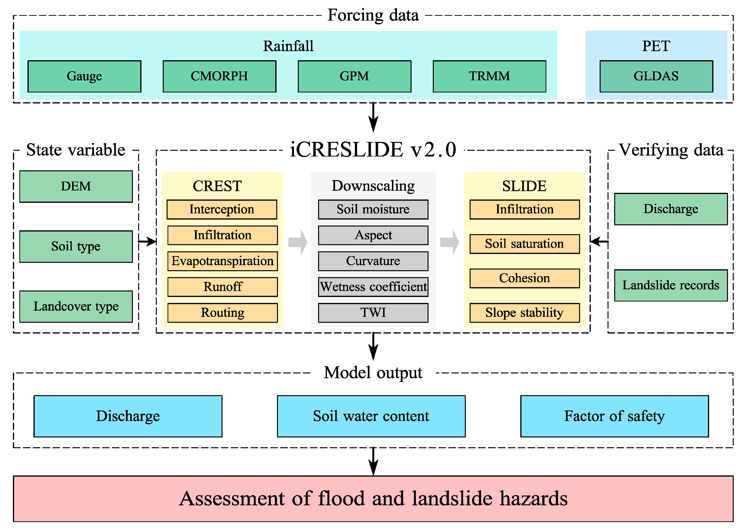
One way to address the inefficiency and termination of the iCRESLIDE model at larger scales is to reduce the spatial resolution of the model. However, this may lead to other issues, such as difficulties in landslide validation. In fact, a previous study has suggested that the appropriate spatial resolution for landslide validation is 90 m [47]. To overcome this issue, an improved version of the iCRESLIDE model, called iCRESLIDE v2.0, has been developed, which introduces a soil moisture downscaling method to couple the hydrological and slope stability models at different spatial scales. In this version, the spatial resolution of the hydrological processes in the CREST model can be set to 1 km, while the spatial resolution of the SLIDE model is set to 90 m or finer. The two models have different spatial resolutions and are related to each other through soil moisture (Figure 2), which is down-scaled using the topographic wetness index (TWI). A detailed description of this method can be found in the study conducted by Wang et al. [22].

2.3.2. Model Performance Evaluation

The iCRESLIDE v2.0 model was utilized to simulate flood and landslide events in the study area only from 2009 to 2012 due to limited data availability, particularly when it came to the landslide inventory data. To compare the impact of different rainfall data on model simulation, the model parameters were first calibrated using gauge rainfall data, following which the model was forced with three other satellite rainfall data sets, using the same parameters as in the calibration procedure. To minimize the impact of the initial state on model simulation, the modeled results from 2010 to 2012 were selected for the model performance evaluation. The model parameters and other inputs were pre-processed before model simulation. A detailed description of the model parameterization can be found in the study conducted by Wang et al. [22].
The metrics used to assess the performance of the hydrological model were the correlation coefficient (Cc) and relative bias. The Cc indicates the degree of relationship between the modeled and observed discharge, while relative bias is often used to measure the degree of deviation. The root mean square error (RMSE) can be also used for the evaluation of model performance; however, the RMSE is sensitive to the abnormal value: for instance, very large modeled discharges. Therefore, it was not adopted in our study. A high Cc and low relative bias suggest that the modeled discharge process is similar to the observation, indicating that the hydrological model has a strong capability to simulate the hydrological process. The Cc and relative bias are expressed as follows:
C c = C o v x , y V a r x V a r y ,
R e l a t i v e   b i a s = 1 n i = 1 n x i y i 1 n i = 1 n y i × 100 % ,
where x is the modeled discharge (m3/s), y is the observed discharge (m3/s), C o v x , y is the covariance between x and y , V a r x and V a r y are the variances of x and y , respectively, and n is the length of the discharge data.
To assess the predictive capability of the SLIDE model for landslide simulation, the Receiver Operating Characteristic (ROC) curve was utilized. The ROC curve indicates whether a binary classification model is effective or not. The binary classification has four possible outcomes: true positive (TP, a landslide is correctly modeled), false positive (FP, a modeled landslide is outside the landslide inventory), true negative (TN, an area is stable for both model prediction and observation), and false negative (FN, a landslide is not captured by the model). Two statistics—true positive rate (TPR, also known as sensitivity) and true negative rate (TNR, also called specificity)—are further defined as follows:
T P R = T P T P + F N ,
T N R = T N T N + F P .
The TPR represents the proportion of correctly predicted landslides, while the TNR is the percentage of negative cases that were accurately predicted. A high TPR indicates that the model captured more landslides, while a high TNR suggests that few modeled landslides were outside the landslide database. The ROC curve comprises TPR and TNR pairs, which are calculated under different cutoff values. In our study, the cutoff variable was the factor of safety (FS). A model performs well if the ROC curve is close to the upper-right corner. The area under the curve (AUC) indicates the overall accuracy of the model. The larger the AUC value, the more accurate the model is in predicting landslides.

3. Results

3.1. Rainfall Analysis

The annual rainfall in the study area was calculated using the four rainfall data sets, as depicted in Figure 3. To facilitate comparison, we use the same legend for all four results in the figure. It is evident that the annual rainfall increases from north to south, with the lowest annual rainfall (of 200 mm) in the northwestern area and the highest (approximately 1200–1400 mm per year) in the southern region. Among the different rainfall data, CMORPH (Figure 3b) presented the lowest annual rainfall, with a regional average of 567 mm, followed by gauge, GPM, and TRMM, with regional averages of 623 mm, 734 mm, and 739 mm, respectively. Additionally, the three satellite rainfall data were all higher than gauge rainfall in the central region, particularly for GPM and TRMM rainfall (Figure 3c,d). CMORPH rainfall was lower than gauge rainfall in the area between the central and southern regions. These findings suggest that the different satellite rainfall data have varying levels of precision in spatial scale, which can impact the simulation of hydrological processes and, ultimately, the predicted slope stability.
The regional daily average rainfall was computed, as presented in Figure 4. Generally, the highest rainfall occurred from July to September, indicating a strong monsoon characteristic. Compared to gauge rainfall (the red dot in Figure 4), CMORPH rainfall (the blue circle in Figure 4) appeared to be lower, while GPM and TRMM rainfall (the pink and green circles in Figure 4, respectively) were higher, consistent with the spatial maps for the four rainfall data sets. The maximum daily rainfalls for gauge, CMORPH, GPM, and TRMM were 32.77 mm, 22.57 mm, 35.32 mm, and 40.75 mm, respectively, suggesting that GPM rainfall is similar to gauge rainfall in extreme situations. The statistics reveal that the Ccs between gauge rainfall and CMORPH, GPM, and TRMM rainfall were 0.63, 0.72, and 0.74, respectively, while the relative biases were −9.02%, 17.70%, and 18.58%, respectively. Although CMORPH rainfall had the lowest relative bias, its Cc was also the lowest. The Ccs for GPM and TRMM rainfall were comparable, but the relative bias of GPM rainfall was lower than that of TRMM rainfall. Furthermore, CMORPH rainfall appeared to be higher in April and May, and this could significantly impact the simulation.
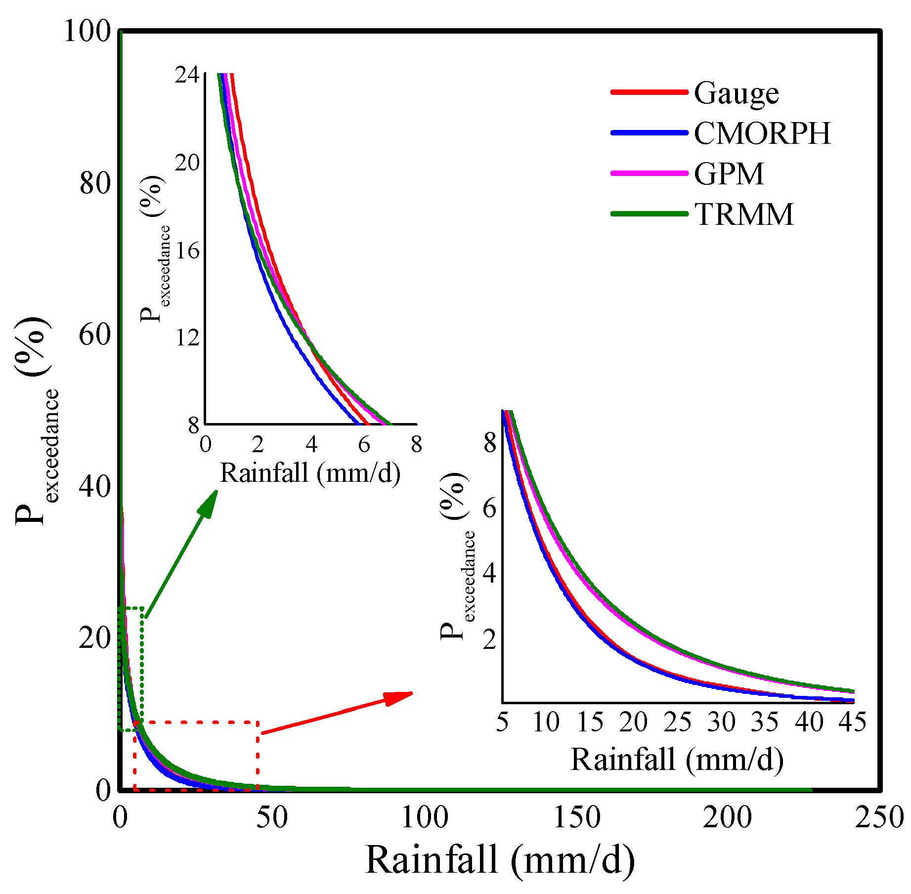
The probability of exceedance for each of the four rainfall data sets was also calculated (Figure 5). CMORPH rainfall was consistently the lowest among the four rainfall data sets. The exceedance probability of gauge rainfall was highest when rainfall was less than 3 mm/d (the upper-left inner chart in Figure 5). As rainfall increased, the exceedance probability of gauge rainfall decreased, approaching that of CMORPH rainfall. The exceedance probability of TRMM rainfall exhibited significant variability: it was lowest when rainfall was less than 1 mm/d but increased substantially and became the highest when rainfall was greater than 4 mm/d (the bottom-right inner chart in Figure 5). This indicates that TRMM rainfall has considerable variation and requires significant improvement in quality. Among the four rainfall data sets, the exceedance probability of GPM rainfall was the most stable. When rainfall was less than 3 mm/d, the exceedance probability of GPM rainfall was closest to that of gauge rainfall, when compared to the exceedance probabilities of CMORPH and TRMM rainfall. However, when rainfall was greater than 5 mm/d, the exceedance probability of GPM rainfall was similar to that of TRMM rainfall, indicating that GPM rainfall generally overestimates actual rainfall during heavy rainfall events. This should be taken into account when using GPM rainfall for research purposes.

3.2. Flood Simulation

Daily discharges at the four hydrological stations were simulated using the iCRESLIDE v2.0 model, as shown in Figure 6. The modeled discharges forced by gauge rainfall (the red virtual line in Figure 6) generally matched the observations well, particularly for Shiquan Station (Figure 6b) and Taoyuan Station (Figure 6d). For the other two hydrological stations, the modeled discharges were close to the observations in the period 2010–2011, but were slightly higher than the observations in 2012. When using different satellite rainfall, the modeled discharges forced by GPM and TRMM rainfall (the pink and green virtual lines in Figure 6, respectively) were significantly higher than the observations, particularly during summer (when rainfall was concentrated and abundant). This finding is consistent with the result that GPM and TRMM tend to overestimate the actual rainfall during heavy rainfall events. Additionally, the differences between modeled discharges by GPM and TRMM rainfall and the observations at Lueyang Station and Shiquan Station (Figure 6a,b) were greater than those at Nanronghua Station and Taoyuan Station (Figure 6c,d). This may be due to the fact that Lueyang Station and Shiquan Station are located in the humid southern region of Shaanxi Province, which receives abundant rainfall during the monsoon season, while Nanronghua Station and Taoyuan Station are situated in the central part of the study area, with only about 500 mm of rainfall per year. Although GPM and TRMM rainfall overestimated the actual rainfall, this overestimation was relatively higher in the south than in the north. The modeled discharges using CMORPH rainfall were generally the smallest among the four rainfall data sets. However, they appeared to be higher in April and May (the blue virtual line in 2011 and 2012 in Figure 6a, in 2010 and 2011 in Figure 6b, in 2011 and 2012 in Figure 6c, and in Figure 6d). This could be attributed to the fact that CMORPH rainfall is higher in spring and often overestimates actual rainfall during this period (the upper-left inner chart in Figure 5), which may explain why the modeled discharge using CMORPH rainfall tended to be higher in spring.
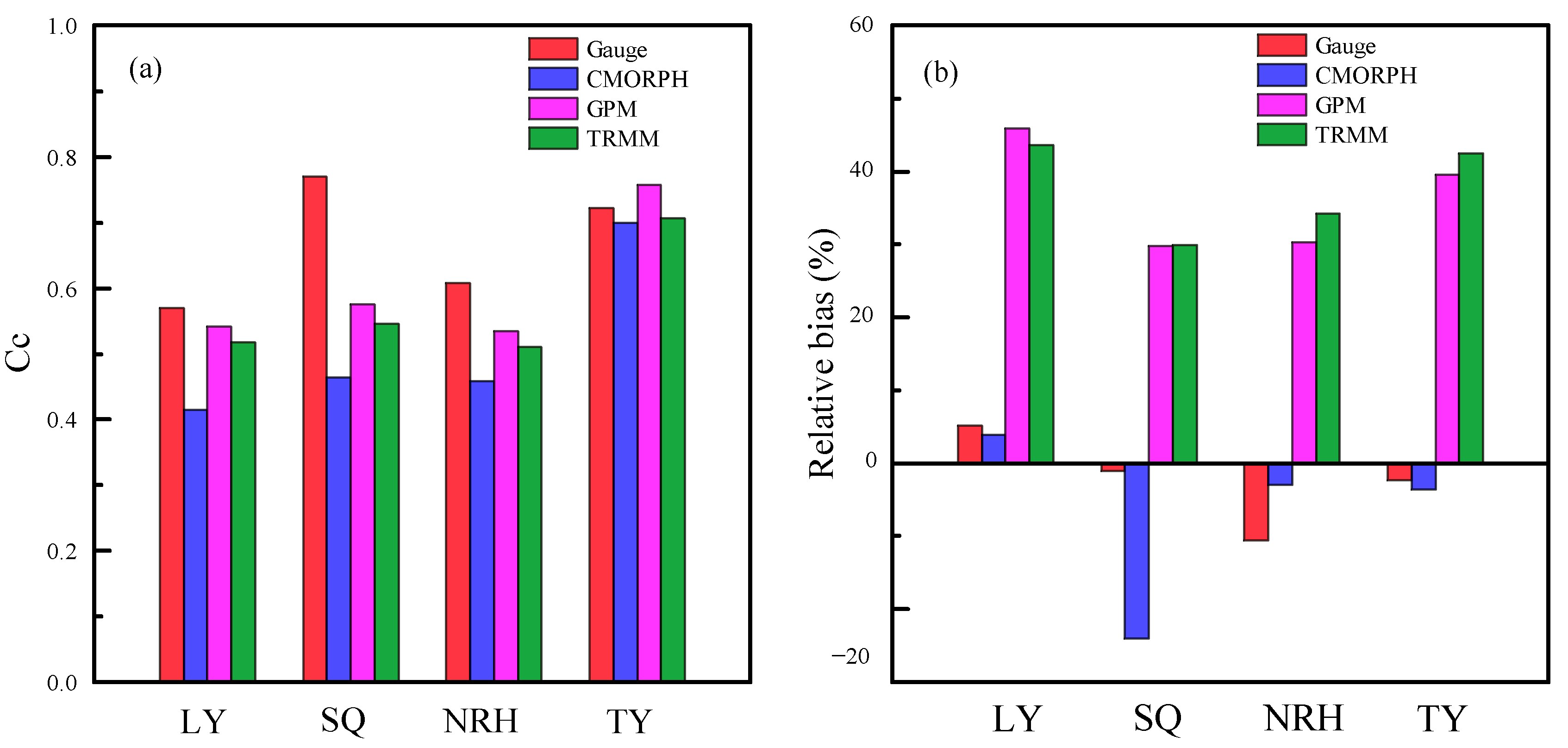
We also calculated the Cc and relative bias of the modeled discharges for the four rainfall data sets at the four hydrological stations (Lueyang Station, Shiquan Station, Nanronghua Station, and Taoyuan Station), as shown in Figure 7. The Ccs of gauge rainfall were 0.57, 0.77, 0.61, and 0.73, while the relative biases were 5.19%, −1.03%, −10.01%, and −2.28%, respectively (i.e., ranging between −10% and 10%). The results indicate that the modeled discharges matched the observations well, and the model simulation was generally accurate. For CMORPH rainfall, the relative biases were 3.85%, −24.01%, −3.00%, and −3.54%, which were smaller than those of GPM and TRMM rainfall. Furthermore, the Ccs of CMORPH rainfall were the lowest among the four rainfall data sets at all four hydrological stations, with values of 0.42, 0.46, 0.45, and 0.70 for Lueyang, Shiquan, Nanronghua, and Taoyuan stations, respectively. For GPM and TRMM, the relative biases were significantly higher than those of gauge rainfall due to the overestimation of rainfall. However, the Ccs of these two satellite rainfall data sets were close to that of gauge rainfall (except at Shiquan Station). Notably, the Cc of GPM rainfall was even higher than that of gauge rainfall at Taoyuan Station (0.76 for GPM rainfall vs. 0.72 for gauge rainfall), indicating that although the bias of modeled discharges using GPM rainfall was greater than that of gauge rainfall, the model simulation forced by GPM rainfall had a strong relationship with the actual hydrological processes.
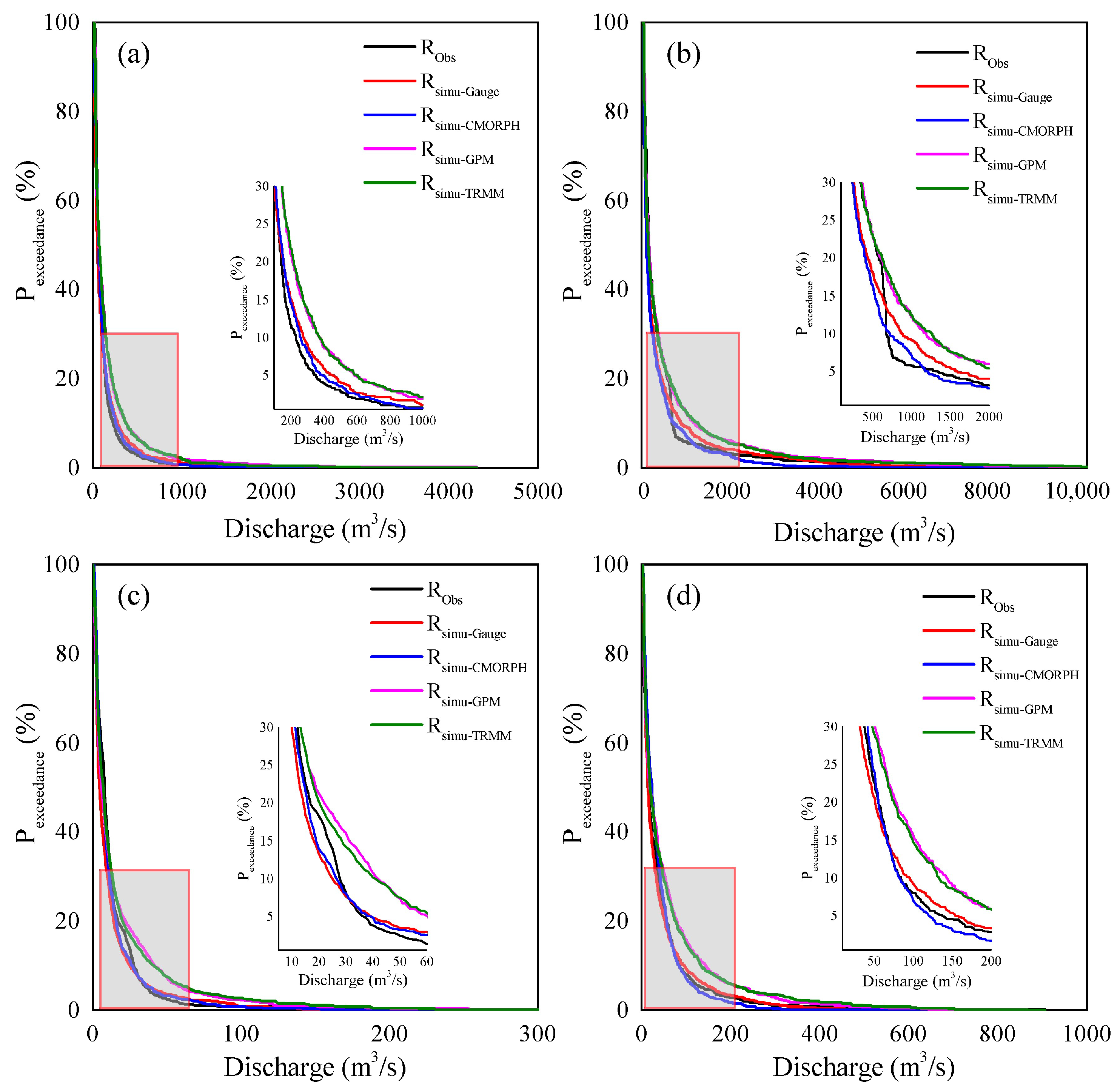
The probability of exceedance of modeled discharges was also calculated, as presented in Figure 8. The exceedance probability of modeled discharges for gauge rainfall (the red line in Figure 8) was generally close to that of the observations, particularly at Lueyang Station and Taoyuan Station (Figure 8a,d); however, for the other two hydrological stations (i.e., Shiquan Station and Nanronghua Station), the exceedance probability lines of the observations exhibited significant variability, especially for Shiquan Station, where the exceedance probability decreased substantially when discharge increased from 600 to 700 m3/s. The exceedance probability of modeled discharges for CMORPH rainfall (the blue line in Figure 8) was generally the lowest among the four rainfall data sets; however, it matched the exceedance probability of observations quite well at low discharge and was close to that of gauge rainfall (Figure 8a,c,d). For GPM and TRMM rainfall, the discharge exceedance probability lines of the two satellite rainfall data sets were quite similar for the four hydrological stations. However, the exceedance probabilities of these two satellite rainfall data sets were both higher than those of the observations, due to rainfall overestimation. Although the exceedance probabilities of modeled discharges using GPM and TRMM rainfall were generally high at the four hydrological stations, they matched the observations well at low discharge, particularly at Shiquan Station (Figure 8b).

3.3. Landslide Simulation

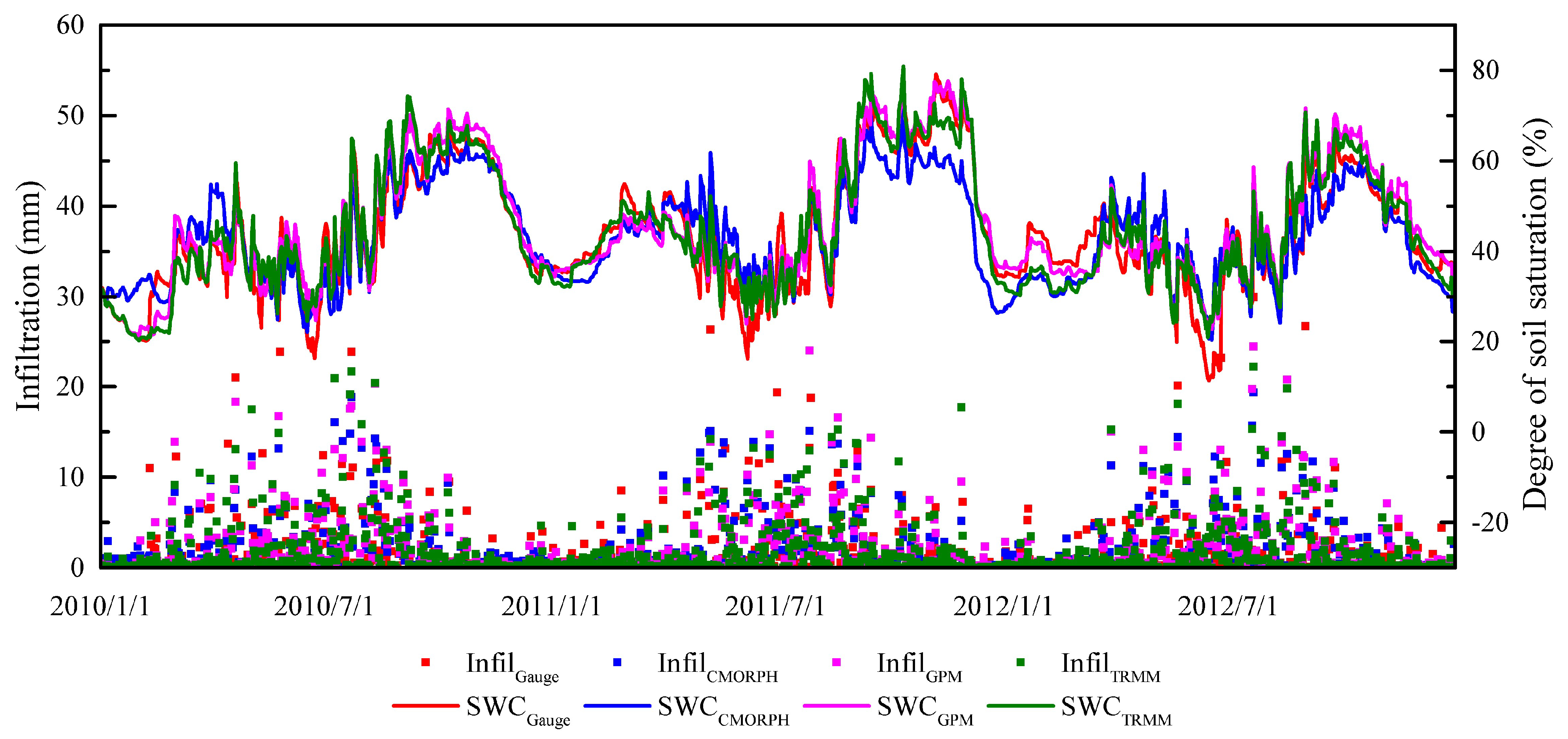
In the iCRESLIDE v2.0 model, slope stability is related to soil water content, which is influenced by rainfall infiltration. To investigate the relationship between rainfall infiltration and soil water content, we calculated the regional average infiltration and degree of soil saturation, as shown in Figure 9. Generally, the infiltration under CMORPH rainfall (blue square) was the lowest, while the infiltration under both GPM and TRMM rainfall (the pink and green squares in Figure 9) was similar to that under gauge rainfall (red square). Despite GPM and TRMM rainfall being greater than gauge rainfall, the infiltration results were not significantly different. This could be due to the fact that the rainfall of all three data sets exceeded the infiltration capacity. The degree of soil saturation has a strong relationship with infiltration, and changes in the degree of soil saturation are similar to those in infiltration, particularly in spring and summer. The soil saturation degree of CMORPH rainfall (blue line) was generally the lowest throughout the study period, except for April and May, consistent with the fact that CMORPH rainfall was high during these months. Additionally, the degree of soil saturation under GPM rainfall (pink line) was similar to that under gauge rainfall (red line), particularly from September to November in 2011, indicating that the simulation of hydrological processes forced by GPM rainfall was similar to that forced by gauge rainfall under the same model parameters. Overall, the results suggest that the iCRESLIDE v2.0 model is capable of capturing the relationship between rainfall infiltration and soil water content, which is crucial for accurately simulating slope stability and landslide hazards.
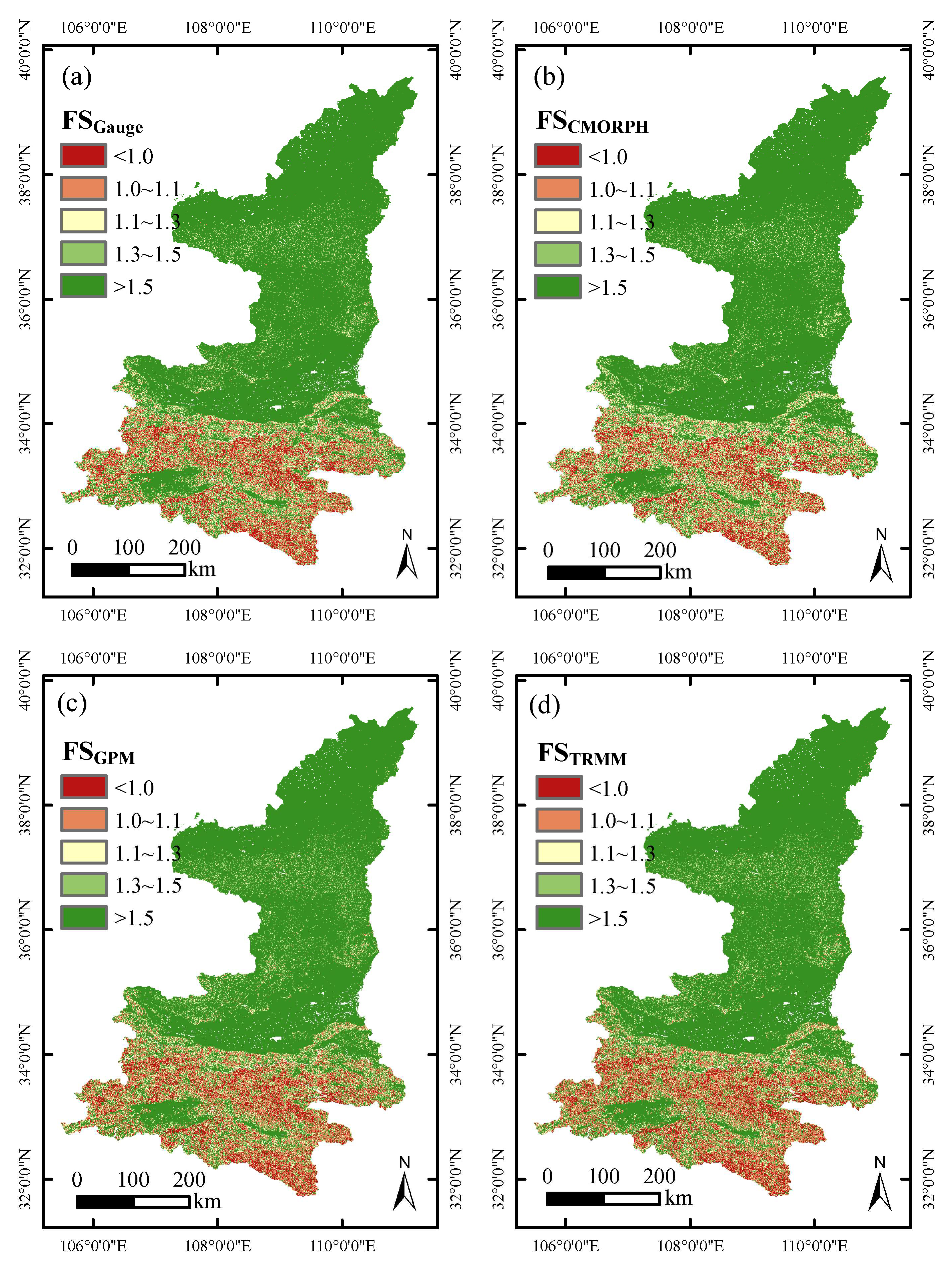
Slope stability is represented as the factor of safety (FS) in the iCRESLIDE v2.0 model. We calculated the minimum FS value for each grid cell during the modeled period in the study area, as shown in Figure 10, for the four rainfall data sets. Compared to Figure 1b, the spatial distributions of FS for all four rainfall data sets matched the landslide inventory map. The FS value was generally low in the south, indicating that landslides are more likely to occur in the southern part of Shaanxi. The FS value was greater than 1.5 in most areas of the central and northern regions, indicating that these areas are the most stable regions of Shaanxi Province. The area between the central and northern regions had a slightly lower FS, due to the relatively steep slopes in this area (see Figure 1b) compared to those in the central and northern regions. In fact, slope is a crucial factor that influences landslides, as it affects soil depth and cohesiveness. A high slope angle increases the likelihood of landslides occurring under the same rainfall conditions compared to a low slope angle [4]. Although the spatial distribution of FS values for different satellite rainfalls was similar to that for gauge rainfall, there were still differences in some areas. For CMORPH rainfall, the area with an FS of less than one accounted for 6.21% of the total area (Figure 10b), and this was smaller than that for gauge rainfall (6.28% of the total area), which is consistent with the fact that CMORPH rainfall was the smallest among the four rainfall data sets. The FS maps of GPM and TRMM rainfall were both similar to that of gauge rainfall, but the FS map of TRMM rainfall presented more red grid cells (Figure 10d), and the percentage of area with FS less than one for TRRM rainfall was 6.32% of the total area, due to the higher rainfall in TRMM. The FS map of GPM rainfall (Figure 10c) was the closest to that of gauge rainfall, with 6.30% of the area having an FS of less than one, indicating that GPM rainfall is more accurate than CMORPH and TRMM rainfall in this regard.
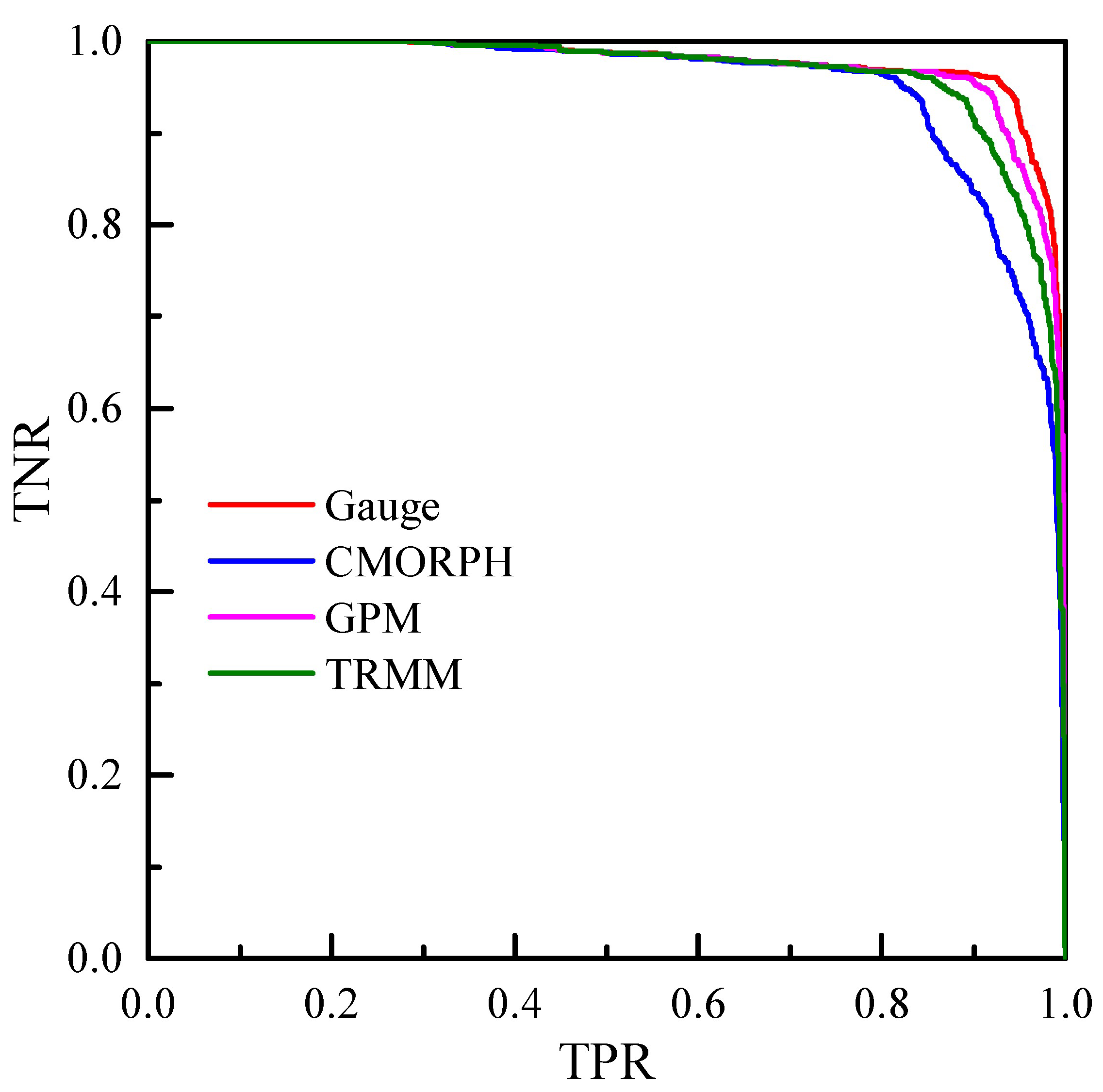
We also calculated the ROC curves of the modeled results derived from the four rainfall data sets (Figure 11). The ROC curve for gauge rainfall was the closest to the upper-right corner, with the greatest AUC value (0.976), indicating that the iCRESLIDE v2.0 model has reliable landslide prediction ability. Moreover, the curve of gauge rainfall had the highest TPR value at the same TNR value among the four curves in most cases, indicating that the model was accurate for not only landslide prediction but also non-landslide simulation. The ROC curve of CMORPH rainfall was the lowest and had the smallest AUC value (0.951), which may have been due to it having the lowest rainfall. The ROC curves of GPM and TRMM rainfall were both close to the upper-right corner, with AUC values of 0.973 and 0.965, respectively. The ROC curve of GPM rainfall was the closest to that of gauge rainfall, when compared to CMORPH and TRMM rainfall, indicating that GPM rainfall has high precision and may be effectively used for regional landslide prediction. Overall, the results suggest that the iCRESLIDE v2.0 model is reliable in landslide prediction, and that the GPM rainfall data can serve as a suitable alternative to gauge rainfall data for regional landslide prediction.

4. Discussion

In this study, we evaluated the effectiveness of different satellite rainfall data sets in terms of hydrological simulation and landslide prediction using the iCRESLIDE v2.0 model. This model was first calibrated using gauge rainfall data, following which CMORPH, GPM, and TRMM rainfall data were used to force the model under the same parameters. As expected, the model performed better when forced by gauge rainfall than when forced by the other three satellite rainfall data sets. However, the results indicated that the performance with GPM rainfall was quite close to that of gauge rainfall for both flood simulation and landslide prediction, showing high Cc and AUC values [48]. This was because GPM rainfall has high accuracy when compared to the other satellite rainfall data sets. The spatiotemporal distribution of GPM rainfall is similar to that of gauge rainfall, leading to better model performance when forced by GPM rainfall [49]. Overall, the results suggest that the GPM rainfall data set can serve as a suitable alternative to gauge rainfall data for hydrological simulation and landslide prediction using the iCRESLIDE v2.0 model.
To further evaluate the performance of the iCRESLIDE v2.0 model in landslide prediction, we compared it with the classical ID (Intensity-Duration) threshold model. We randomly selected grid cells that experienced three times the normal number of landslide events, then calculated the rainfall intensity and duration for these landslide and non-landslide grid cells. The time step of the iCRESLIDE v2.0 model used in our study is one day, and so we defined a rainfall event as continuous rainfall or discontinued rain with non-rain intermittent periods of less than or equal to one day. To account for the impact of antecedent rainfall on landslide occurrence, we calculated the effective rainfall according to the widely used exponential form method, which can be expressed as follows:
P e = i = 0 n α i P i ,
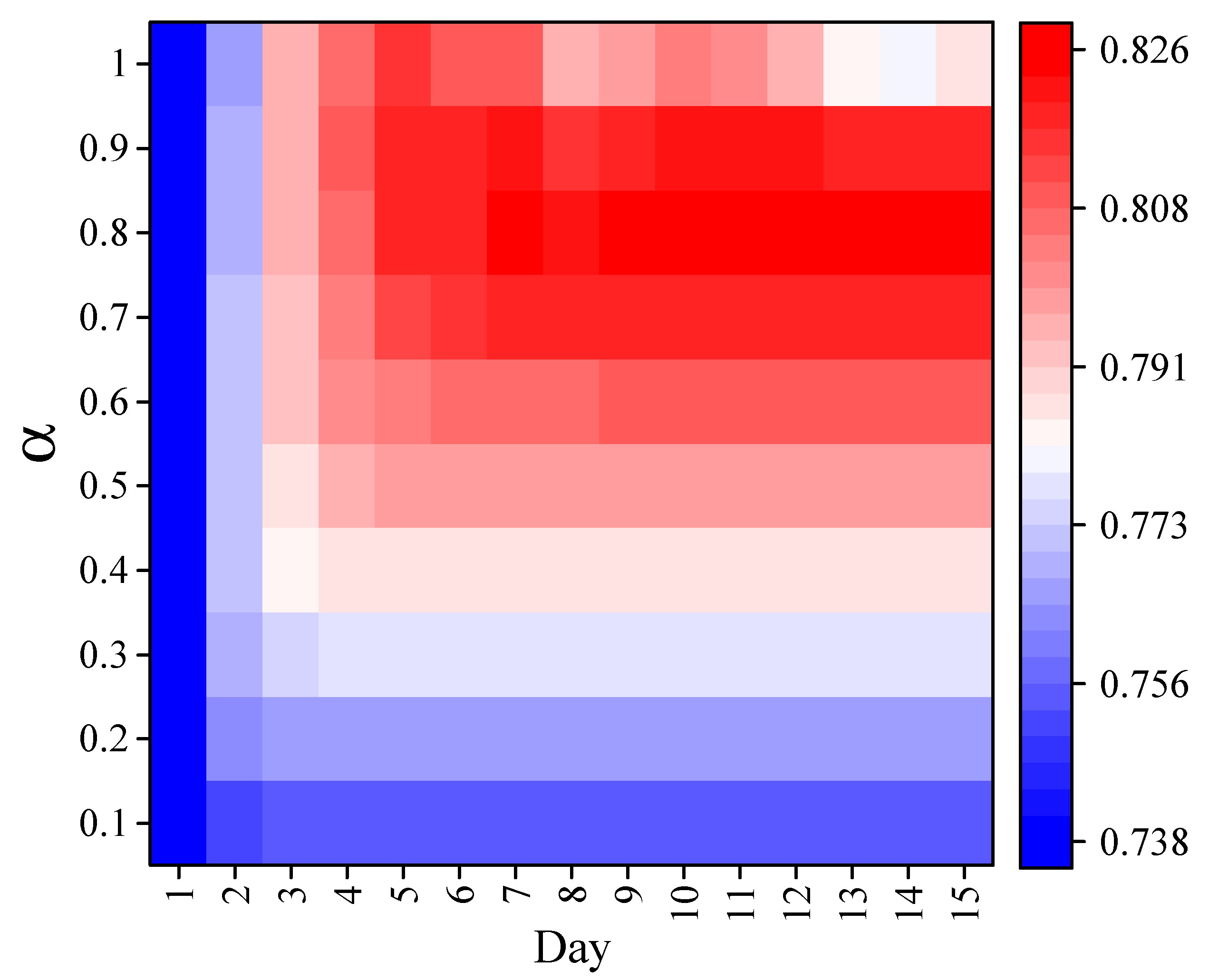
where P e is the effective rainfall, n is the rainfall duration, α is the coefficient of effective rainfall, and P i denotes the i th day’s rainfall before the landslide event. The value of α can vary in different regions. Therefore, we calculated the Cc of effective rainfall and landslide events under different values of α and different antecedent days, as shown in Figure 12. The results indicate that the Cc is highest when α is equal to 0.8 and the antecedent day is 12. Therefore, we determined the coefficient of effective rainfall to be 0.8.
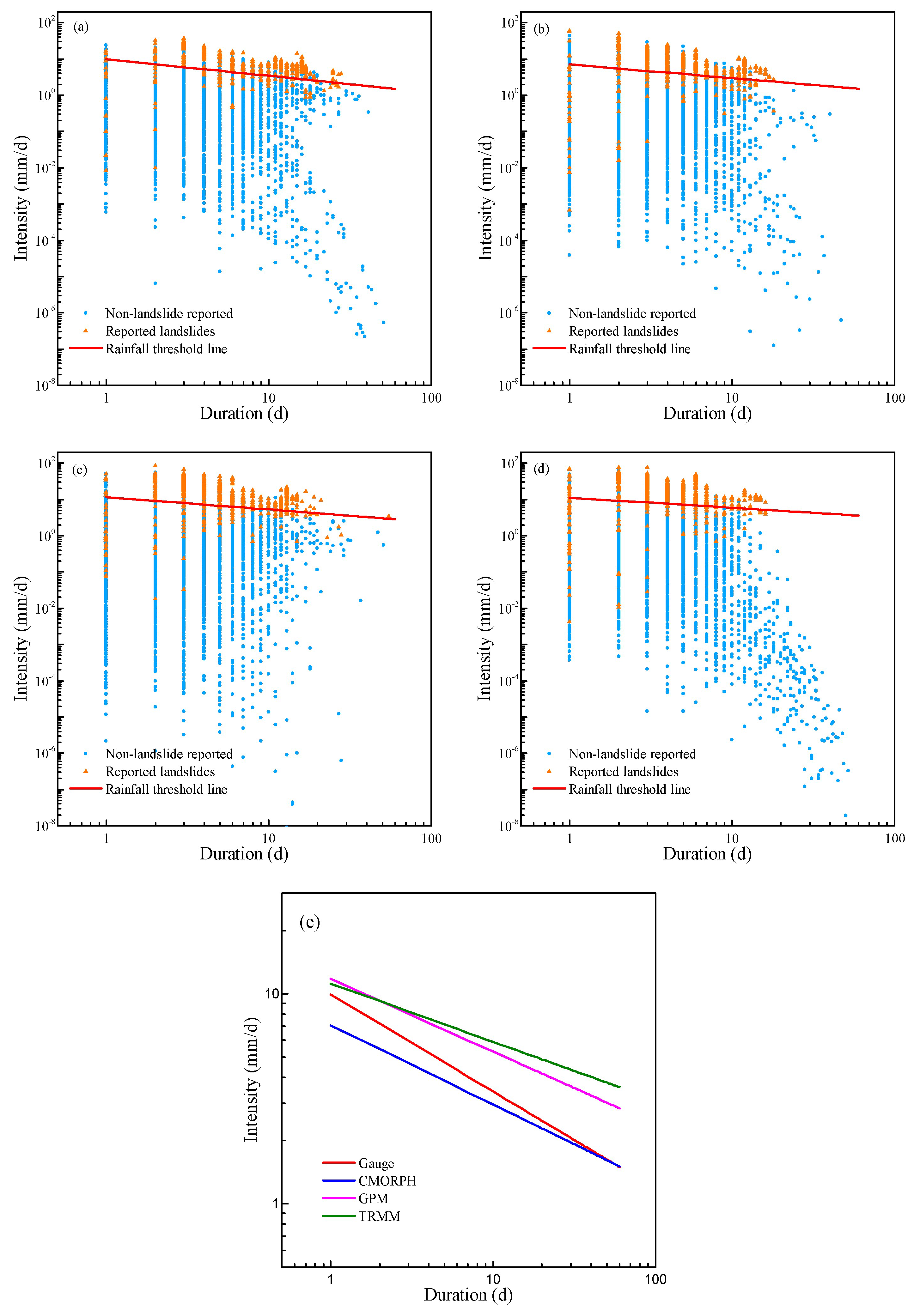
We calculated the rainfall volume, duration, and intensity for each landslide and non-landslide grid cell. The rainfall threshold line was then calculated using a linear regression model and adjusted by its intercept in order to ensure that 90% of the total grid cells were predicted correctly by the ID model (the red lines in Figure 13a–d). The ID models for the four rainfall data sets are shown in Figure 13e, and the equations are listed in Table 1. The threshold line for CMORPH rainfall was the lowest, with a slope of −0.378 and an intercept of 0.850, while the threshold line of TRMM rainfall was the highest, with a slope of −0.277 and an intercept of 1.048; these values were consistent with the results of the rainfall analysis. The threshold line of GPM rainfall was the closest to that of gauge rainfall, with almost equal intercepts (1.070 for GPM rainfall vs. 0.995 for gauge rainfall) and similar slopes (−0.346 for GPM rainfall vs. −0.461 for gauge rainfall). These results further support the notion that GPM rainfall has good quality and landslide prediction ability.
We also calculated the AUC values of the ROC curves for the ID models (Table 2). Generally, the AUC values for the ID models were lower than those for the iCRESLIDE v2.0 models for all rainfall data sets. The gauge rainfall had the highest AUC values for both the iCRESLIDE v2.0 and ID models, with values of 0.976 and 0.860, respectively. The AUC values of GPM rainfall were the highest among the three satellite rainfall data sets (0.973 vs. 0.951 and 0.965 for the iCRESLIDE v2.0 model and 0.566 vs. 0.546 and 0.408 for the ID model), indicating that GPM rainfall had the best landslide prediction ability. Moreover, the higher AUC values of the iCRESLIDE v2.0 model suggest that this physically based model is more robust than the ID model. The iCRESLIDE v2.0 model has good adaptability to different situations and to forcing data.

5. Conclusions

In this study, we aimed to explore the effectiveness of different satellite rainfall data sets in flood and landslide simulation using the iCRESLIDE v2.0 model. The results demonstrated that the CMORPH, GPM, and TRMM rainfall data sets performed well in flood simulation and landslide prediction, yielding high Cc and AUC values. Among the three satellite rainfall data sets, GPM rainfall presented the best performance, with good model simulation quality and ability. Moreover, the physically based iCRESLIDE v2.0 model was found to be more robust than the ID threshold model, which is a statistical method. The strong applicability of the considered model and the wide availability of satellite rainfall data can provide beneficial and efficient results for the prediction of floods and landslides over large regions, reducing the damages caused by these hazards and providing effective countermeasures for disaster management departments.
However, this study has some limitations that need to be addressed and resolved in future research. One limitation is that satellite rainfall data may have biases compared to gauge rainfall data, and this can affect the accuracy of the model. To obtain more accurate rainfall data, correction methods for satellite rainfall, such as the multi-source rainfall fusion method [50,51], have been proposed by many researchers, and applying these methods could improve the performance of the developed model. Additionally, with the development of new techniques, satellite rainfall data sets are becoming more abundant. Newly available satellite rainfall data sets are expected to have higher accuracy and can be better utilized in such models. Therefore, future research should focus on improving the accuracy of satellite rainfall data and exploring new techniques to enhance the performance of the model in use.

Author Contributions

Conceptualization, S.W. and K.Z.; Funding acquisition, S.W. and K.Z.; Methodology, S.W. and L.C.; Supervision, K.Z. and L.C.; Validation, S.W., G.C. and Y.X.; Visualization, S.W. and C.Z.; Writing—original draft, S.W.; Writing—review & editing, S.W., K.Z. and L.C. All authors have read and agreed to the published version of the manuscript.

Funding

This research was funded by the National Natural Science Foundation of China (522031511, 51879067, 52009028) and the Fundamental Research Funds for the Central Universities (B220202029, B220204014).

Data Availability Statement

Gauge rainfall data were provided by China Meteorological Administration (http://data.cma.cn, accessed on 1 January 2017). CMORPH rainfall data were downloaded from the National Centers for Environmental Information of National Oceanic and Atmospheric Administration (https://www.ncei.noaa.gov/products/climate-data-records/precipitation-cmorph, accessed on 1 June 2017). GPM rainfall data were downloaded from the National Aeronautics and Space Administration (https://gpm.nasa.gov/data, accessed on 27 February 2014). TRMM rainfall data were downloaded from the National Aeronautics and Space Administration (https://gpm.nasa.gov/missions/trmm, accessed on 27 November 1997). The potential evapotranspiration data were provided by Global Land Data Assimilation System (GLDAS, https://ldas.gsfc.nasa.gov/gldas/GLDASdownload.php, accessed on 1 March 2004). The DEM data with 90 m resolution were provided by the Geospatial Data Cloud site, Computer Network Information Center, Chinese Academy of Sciences (http://www.gscloud.cn, accessed on 6 January 2015). The DEM data with 1 km resolution were provided by HydroSHEDS (https://hydrosheds.org/pages/availability, accessed on 4 March 2008). The land cover data were derived from GlobeLand30-2010, which is a product of global land cover at a spatial resolution of 30 m derived from remote-sensing images in 2010 (http://www.globeland30.cn, accessed on 1 May 2014). The soil data were obtained from the Harmonized World Soil Database (HWSD) v1.2 (https://daac.ornl.gov/SOILS/guides/HWSD.html, accessed on 15 September 2014). The landslide hazard data were obtained from the geological survey office of the Department of Land and Resources of Shaanxi Province. The discharge data were digitalized from Hydrological Year Books.

Conflicts of Interest

The authors declare no conflict of interest.

References

  1. An, H.; Viet, T.T.; Lee, G.; Kim, Y.; Kim, M.; Noh, S.; Noh, J. Development of time-variant landslide-prediction software considering three-dimensional subsurface unsaturated flow. Environ. Model. Softw. 2016, 85, 172–183. [Google Scholar] [CrossRef]
  2. Huang, X.; Li, Z.; Yu, D.; Xu, Q.; Fan, J.; Hao, Z.; Niu, Y. Evolution of a giant debris flow in the transitional mountainous region between the Tibetan Plateau and the Qinling Mountain range, Western China: Constraints from broadband seismic records. J. Asian Earth Sci. 2017, 148, 181–191. [Google Scholar] [CrossRef]
  3. Chen, J.; Zeng, Z.; Jiang, P.; Tang, H. Deformation prediction of landslide based on functional network. Neurocomputing 2015, 149, 151–157. [Google Scholar] [CrossRef]
  4. Zhang, K.; Wang, S.; Bao, H.; Zhao, X. Characteristics and influencing factors of rainfall-induced landslide and debris flow hazards in Shaanxi Province, China. Nat. Hazards Earth Syst. Sci. 2019, 19, 93–105. [Google Scholar] [CrossRef]
  5. Burnash, R.J.; Ferral, R.L.; McGuire, R.A. A Generalized Streamflow Simulation System: Conceptual Modeling for Digital Computers; US Department of Commerce, National Weather Service, and State of California: Los Angeles, CA, USA, 1973.
  6. Crawford, N.H.; Linsley, R.K. Digital Simulation in Hydrology’Stanford Watershed Model 4; Technical Report; Stanford University: Stanford, CA, USA, 1966. [Google Scholar]
  7. Sugawara, M.; Watanabe, I.; Ozaki, E.; Katsugama, Y. Tank Model with Snow Component; Research Notes of the National Research Center for Disaster Prevention No. 65; Science and Technolgoy: Ibaraki-Ken, Japan, 1984. [Google Scholar]
  8. BEVEN, K.J.; Kirkby, M.J. A physically based, variable contributing area model of basin hydrology/Un modèle à base physique de zone d’appel variable de l’hydrologie du bassin versant. Hydrol. Sci. J. 1979, 24, 43–69. [Google Scholar] [CrossRef]
  9. Duan, J.; Miller, N.L. A generalized power function for the subsurface transmissivity profile in TOPMODEL. Water Resour. Res. 1997, 33, 2559–2562. [Google Scholar] [CrossRef]
  10. Abbott, M.B.; Bathurst, J.C.; Cunge, J.A.; O’Connell, P.E.; Rasmussen, J. An introduction to the European Hydrological System—Systeme Hydrologique Europeen, “SHE”, 1: History and philosophy of a physically-based, distributed modelling system. J. Hydrol. 1986, 87, 45–59. [Google Scholar] [CrossRef]
  11. Giannaros, C.; Dafis, S.; Stefanidis, S.; Giannaros, T.M.; Koletsis, I.; Oikonomou, C. Hydrometeorological analysis of a flash flood event in an ungauged Mediterranean watershed under an operational forecasting and monitoring context. Meteorol. Appl. 2022, 29, e2079. [Google Scholar] [CrossRef]
  12. Quenum, G.M.L.D.; Arnault, J.; Klutse, N.A.B.; Zhang, Z.; Kunstmann, H.; Oguntunde, P.G. Potential of the coupled WRF/WRF-hydro modeling system for flood forecasting in the Ouémé River (West Africa). Water 2022, 14, 1192. [Google Scholar] [CrossRef]
  13. Fookes, P. Geology for engineers: The geological model, prediction and performance. Q. J. Eng. Geol. Hydrogeol. 1997, 30, 293–424. [Google Scholar] [CrossRef]
  14. Guzzetti, F.; Cardinali, M.; Reichenbach, P.; Carrara, A. Comparing Landslide Maps: A Case Study in the Upper Tiber River Basin, Central Italy. Environ. Manag. 2000, 25, 247–263. [Google Scholar] [CrossRef]
  15. Griffiths, J.S. Mapping in Engineering Geology; Geological Society of London: London, UK, 2002. [Google Scholar]
  16. Glade, T.; Crozier, M.; Smith, P. Applying probability determination to refine landslide-triggering rainfall thresholds using an empirical “Antecedent Daily Rainfall Model”. Pure Appl. Geophys. 2000, 157, 1059–1079. [Google Scholar] [CrossRef]
  17. Guzzetti, F.; Peruccacci, S.; Rossi, M.; Stark, C.P. The rainfall intensity–duration control of shallow landslides and debris flows: An update. Landslides 2008, 5, 3–17. [Google Scholar] [CrossRef]
  18. Bogaard, T.; Greco, R. Hydrological perspectives on precipitation intensity-duration thresholds for a landslide initiation: Proposing hydro-meteorological thresholds. Nat. Hazards Earth Syst. Sci. 2018, 18, 31–39. [Google Scholar] [CrossRef]
  19. Montrasio, L.; Valentino, R. A model for triggering mechanisms of shallow landslides. Nat. Hazards Earth Syst. Sci. 2008, 8, 1149–1159. [Google Scholar] [CrossRef]
  20. Liao, Z.; Hong, Y.; Wang, J.; Fukuoka, H.; Sassa, K.; Karnawati, D.; Fathani, F. Prototyping an experimental early warning system for rainfall-induced landslides in Indonesia using satellite remote sensing and geospatial datasets. Landslides 2010, 7, 317–324. [Google Scholar] [CrossRef]
  21. Zhang, K.; Xue, X.; Hong, Y.; Gourley, J.J.; Lu, N.; Wan, Z.; Hong, Z.; Wooten, R. iCRESTRIGRS: A coupled modeling system for cascading flood–landslide disaster forecasting. Hydrol. Earth Syst. Sci. 2016, 20, 5035–5048. [Google Scholar] [CrossRef]
  22. Wang, S.; Zhang, K.; van Beek, L.P.; Tian, X.; Bogaard, T.A. Physically-based landslide prediction over a large region: Scaling low-resolution hydrological model results for high-resolution slope stability assessment. Environ. Model. Softw. 2020, 124, 104607. [Google Scholar] [CrossRef]
  23. He, X.; Hong, Y.; Vergara, H.; Zhang, K.; Kirstetter, P.-E.; Gourley, J.J.; Zhang, Y.; Qiao, G.; Liu, C. Development of a coupled hydrological-geotechnical framework for rainfall-induced landslides prediction. J. Hydrol. 2016, 543, 395–405. [Google Scholar] [CrossRef]
  24. Michelson, D.B. Systematic correction of precipitation gauge observations using analyzed meteorological variables. J. Hydrol. 2004, 290, 161–177. [Google Scholar] [CrossRef]
  25. Renard, B.; Kavetski, D.; Kuczera, G.; Thyer, M.; Franks, S.W. Understanding predictive uncertainty in hydrologic modeling: The challenge of identifying input and structural errors. Water Resour. Res. 2010, 46, 1–22. [Google Scholar] [CrossRef]
  26. Qi, Y.; Zhang, J. Correction of radar QPE errors associated with low and partially observed brightband layers. J. Hydrometeorol. 2013, 14, 1933–1943. [Google Scholar] [CrossRef]
  27. Hsu, K.-L.; Gao, X.; Sorooshian, S.; Gupta, H.V. Precipitation estimation from remotely sensed information using artificial neural networks. J. Appl. Meteorol. 1997, 36, 1176–1190. [Google Scholar] [CrossRef]
  28. Alahacoon, N.; Matheswaran, K.; Pani, P.; Amarnath, G. A decadal historical satellite data and rainfall trend analysis (2001–2016) for flood hazard mapping in Sri Lanka. Remote Sens. 2018, 10, 448. [Google Scholar] [CrossRef]
  29. Toté, C.; Patricio, D.; Boogaard, H.; Van Der Wijngaart, R.; Tarnavsky, E.; Funk, C. Evaluation of satellite rainfall estimates for drought and flood monitoring in Mozambique. Remote Sens. 2015, 7, 1758–1776. [Google Scholar] [CrossRef]
  30. Adane, G.B.; Hirpa, B.A.; Lim, C.-H.; Lee, W.-K. Evaluation and comparison of satellite-derived estimates of rainfall in the diverse climate and terrain of central and northeastern Ethiopia. Remote Sens. 2021, 13, 1275. [Google Scholar] [CrossRef]
  31. Kummerow, C.; Barnes, W.; Kozu, T.; Shiue, J.; Simpson, J. The tropical rainfall measuring mission (TRMM) sensor package. J. Atmos. Ocean. Technol. 1998, 15, 809–817. [Google Scholar] [CrossRef]
  32. Ushio, T.; Okamoto, K.i.; Iguchi, T.; Takahashi, N.; Iwanami, K.; Aonashi, K.; Shige, S.; Hashizume, H.; Kubota, T.; Inoue, T. The global satellite mapping of precipitation (GSMaP) project. Aqua AMSR-E 2003, 2004, 1–2. [Google Scholar]
  33. Joyce, R.J.; Janowiak, J.E.; Arkin, P.A.; Xie, P. CMORPH: A method that produces global precipitation estimates from passive microwave and infrared data at high spatial and temporal resolution. J. Hydrometeorol. 2004, 5, 487–503. [Google Scholar] [CrossRef]
  34. Huffman, G.J.; Bolvin, D.T.; Braithwaite, D.; Hsu, K.; Joyce, R.; Xie, P.; Yoo, S.-H. NASA global precipitation measurement (GPM) integrated multi-satellite retrievals for GPM (IMERG). Algorithm Theor. Basis Doc. ATBD Version 2015, 4, 1–39. [Google Scholar]
  35. Hong, Y.; Hsu, K.L.; Sorooshian, S.; Gao, X. Improved representation of diurnal variability of rainfall retrieved from the Tropical Rainfall Measurement Mission microwave imager adjusted Precipitation Estimation from Remotely Sensed Information Using Artificial Neural Networks (PERSIANN) system. J. Geophys. Res. Atmos. 2005, 110, D06012. [Google Scholar] [CrossRef]
  36. Griffith, C.G.; Woodley, W.L.; Grube, P.G.; Martin, D.W.; Stout, J.; Sikdar, D.N. Rain estimation from geosynchronous satellite imagery—Visible and infrared studies. Mon. Weather Rev. 1978, 106, 1153–1171. [Google Scholar] [CrossRef]
  37. Fang, J.; Yang, W.; Luan, Y.; Du, J.; Lin, A.; Zhao, L. Evaluation of the TRMM 3B42 and GPM IMERG products for extreme precipitation analysis over China. Atmos. Res. 2019, 223, 24–38. [Google Scholar] [CrossRef]
  38. Yu, L.; Leng, G.; Python, A.; Peng, J. A comprehensive evaluation of latest GPM IMERG V06 early, late and final precipitation products across China. Remote Sens. 2021, 13, 1208. [Google Scholar] [CrossRef]
  39. Shen, Y.; Xiong, A.; Wang, Y.; Xie, P. Performance of high-resolution satellite precipitation products over China. J. Geophys. Res. Atmos. 2010, 115, D02114. [Google Scholar] [CrossRef]
  40. Getirana, A.; Kirschbaum, D.; Mandarino, F.; Ottoni, M.; Khan, S.; Arsenault, K. Potential of GPM IMERG precipitation estimates to monitor natural disaster triggers in urban areas: The case of Rio de Janeiro, Brazil. Remote Sens. 2020, 12, 4095. [Google Scholar] [CrossRef]
  41. Krige, D.G. A Statistical Approach to Some Mine Valuation and Allied Problems on the Witwatersrand: By DG Krige; University of the Witwatersrand: Johannesburg, South Africa, 1951. [Google Scholar]
  42. Rodell, M.; Houser, P.; Jambor, U.; Gottschalck, J.; Mitchell, K.; Meng, C.-J.; Arsenault, K.; Cosgrove, B.; Radakovich, J.; Bosilovich, M. The global land data assimilation system. Bull. Am. Meteorol. Soc. 2004, 85, 381–394. [Google Scholar] [CrossRef]
  43. Lehner, B.; Verdin, K.; Jarvis, A. New global hydrography derived from spaceborne elevation data. Eos Trans. Am. Geophys. Union 2008, 89, 93–94. [Google Scholar] [CrossRef]
  44. Wieder, W.; Boehnert, J.; Bonan, G.; Langseth, M. Regridded Harmonized World Soil Database v1. 2. ORNL DAAC. 2014. Available online: https://daac.ornl.gov/SOILS/guides/HWSD.html (accessed on 15 September 2014).
  45. Chen, J.; Chen, J.; Liao, A.; Cao, X.; Chen, L.; Chen, X.; He, C.; Han, G.; Peng, S.; Lu, M. Global land cover mapping at 30 m resolution: A POK-based operational approach. ISPRS J. Photogramm. Remote Sens. 2015, 103, 7–27. [Google Scholar] [CrossRef]
  46. Wang, J.; Hong, Y.; Li, L.; Gourley, J.J.; Khan, S.I.; Yilmaz, K.K.; Adler, R.F.; Policelli, F.S.; Habib, S.; Irwn, D. The coupled routing and excess storage (CREST) distributed hydrological model. Hydrol. Sci. J. 2011, 56, 84–98. [Google Scholar] [CrossRef]
  47. Tian, Y.; XiaO, C.; Liu, Y.; Wu, L. Effects of raster resolution on landslide susceptibility mapping: A case study of Shenzhen. Sci. China Ser. E Technol. Sci. 2008, 51, 188–198. [Google Scholar] [CrossRef]
  48. Guo, Z.; Ferrer, J.V.; Hürlimann, M.; Medina, V.; Puig-Polo, C.; Yin, K.; Huang, D. Shallow landslide susceptibility assessment under future climate and land cover changes: A case study from southwest China. Geosci. Front. 2023, 14, 101542. [Google Scholar] [CrossRef]
  49. Ozturk, U.; Saito, H.; Matsushi, Y.; Crisologo, I.; Schwanghart, W. Can global rainfall estimates (satellite and reanalysis) aid landslide hindcasting? Landslides 2021, 18, 3119–3133. [Google Scholar] [CrossRef]
  50. Chao, L.; Zhang, K.; Li, Z.; Zhu, Y.; Wang, J.; Yu, Z. Geographically weighted regression based methods for merging satellite and gauge precipitation. J. Hydrol. 2018, 558, 275–289. [Google Scholar] [CrossRef]
  51. Ma, Y.; Yang, Y.; Han, Z.; Tang, G.; Maguire, L.; Chu, Z.; Hong, Y. Comprehensive evaluation of ensemble multi-satellite precipitation dataset using the dynamic bayesian model averaging scheme over the Tibetan Plateau. J. Hydrol. 2018, 556, 634–644. [Google Scholar] [CrossRef]
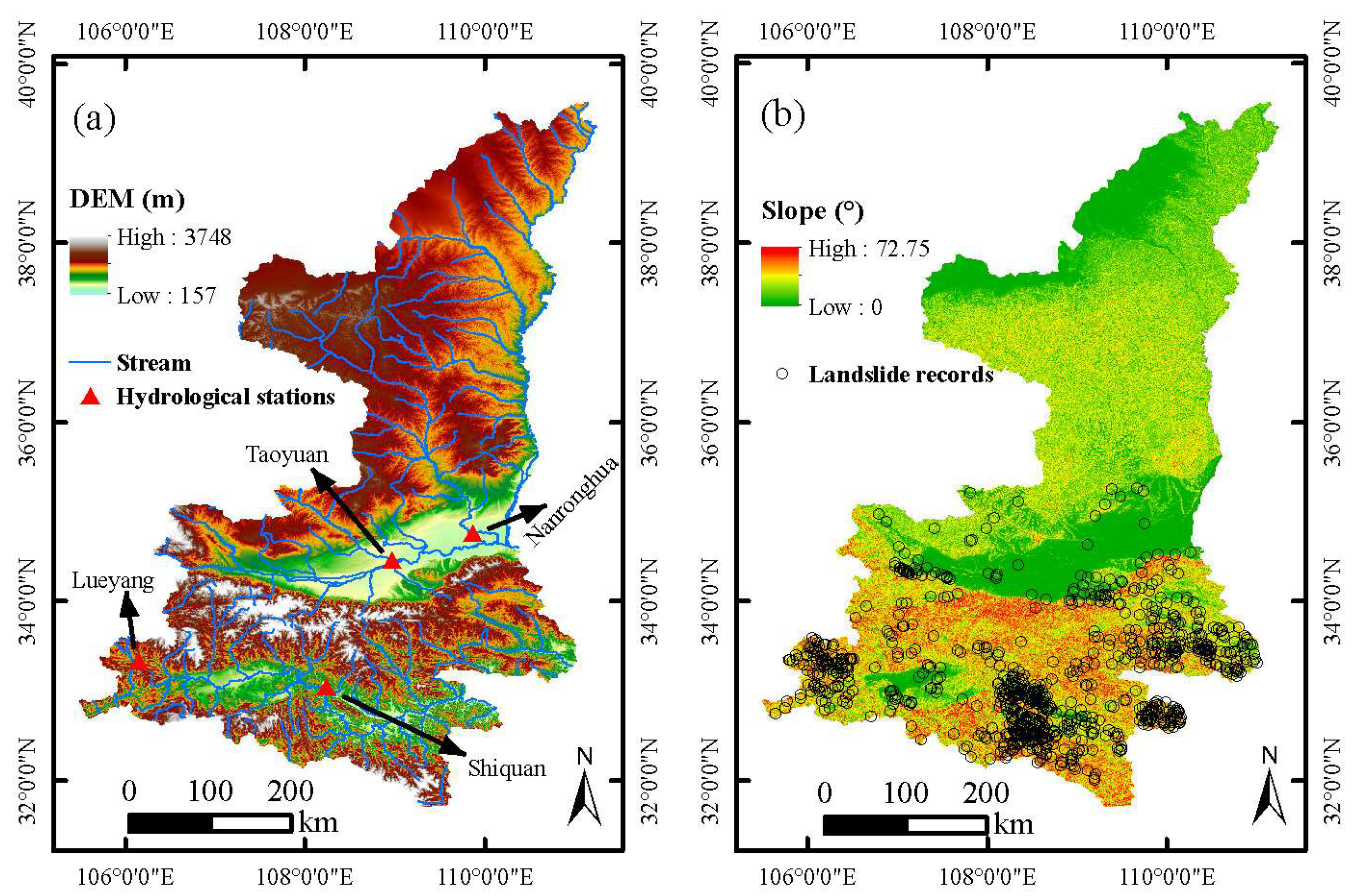
Figure 1. Maps of (a) DEM and (b) slope of Shaanxi Province, associated with streams and landslide records, respectively.
Remotesensing 15 02457 g001
Figure 2. Flowchart of the methodology in the study.
Remotesensing 15 02457 g002
Figure 3. Spatial distribution of annual rainfall: (a) Gauge; (b) CMORPH; (c) GPM; and (d) TRMM.
Remotesensing 15 02457 g003
Figure 4. Regional average rainfall for the four rainfall data sets in time-series form.
Remotesensing 15 02457 g004
Figure 5. Probability of rainfall exceedance for the four rainfall data sets.
Remotesensing 15 02457 g005
Figure 6. Observed and modeled daily discharges forced by the four rainfall data sets at the four hydrological stations: (a) Lueyang Station; (b) Shiquan Station; (c) Nanronghua Station; and (d) Taoyuan Station.
Remotesensing 15 02457 g006
Figure 7. Evaluation metrics of: (a) Cc and (b) relative bias of modeled discharges for the four rainfall data sets at four hydrological stations. Here LY, SQ, NRH, and TY are the short forms of Lueyang, Shiquan, Nanronghua, and Taoyuan, respectively.
Remotesensing 15 02457 g007
Figure 8. Probability of exceedance for observed and modeled discharges for the four rainfall data sets: (a) Lueyang Station; (b) Shiquan Station; (c) Nanronghua Station; and (d) Taoyuan Station.
Remotesensing 15 02457 g008
Figure 9. Modeled results of regional average rainfall infiltration and degree of soil saturation in time series (here, Infil represents infiltration and SWC denotes soil water content).
Remotesensing 15 02457 g009
Figure 10. Minimum FS of the study area during the modeled period: (a) Gauge; (b) CMORPH; (c) GPM; and (d) TRMM.
Remotesensing 15 02457 g010
Figure 11. ROC curves modeled by the four rainfall data sets.
Remotesensing 15 02457 g011
Figure 12. Heat map of Cc between rainfall and landslide under a varying number of antecedent days and different effective rainfall coefficients.
Remotesensing 15 02457 g012
Figure 13. Rainfall threshold lines of ID model: (a) Gauge; (b) CMORPH; (c) GPM; and (d) TRMM rainfall. All the four threshold lines are shown in sub-figure (e) in order to compare these lines directly.
Remotesensing 15 02457 g013
Table 1. Data sets used in the study and their pre-processing.
VariableData SetPre-Processing
RainfallGaugeThe data were interpolated into a resolution of 1 km grid data via the Kriging method.
CMORPHThe daily rainfall data were interpolated into a resolution of 1 km via the bilinear method.
GPMThe hourly rainfall data were aggregated into daily scale and further interpolated into 1 km resolution through the bilinear method.
TRMMThe daily rainfall data were interpolated into a resolution of 1 km via the bilinear method.
PETGLDASThese data are in a spatial resolution of 0.25 degree and their time interval is 3 h. We interpolated them into 1 km resolution by using the bilinear method and cumulated them to daily scale.
DEM1 km-resolution DEM were from Hydrological data maps based on HydroSHEDSThe 1 km DEM of the study area was extracted from the original data.
90 m-resolution DEM were from the Geospatial Data Cloud.The 90 m DEM of the study area was extracted from the original data.
Land cover typeGlobeLand30-2010The original 30 m data set was resampled to 1 km and 90 m resolution for being applied in the hydrological model and slope stability model, respectively.
Soil typeHarmonized World Soil Database (HWSD) v1.2This data was resampled to 90 m resolution when used in slope stability model.
DischargeHydrological Year BooksThe daily discharge data were arranged according to the hydrological stations.
Landslide inventoryThe landslide inventory data were obtained from the Geological Survey Office of the Department of Land and Resources of Shaanxi ProvinceThe information on location, occurrence time, and triggering factor was selected for each landslide record.
Table 2. AUC values of iCRESLIDE v2.0 and ID models, as well as ID model equations.
RainfallAUC of SLIDE ModelAUC of ID ModelEquation of ID Model
Gauge0.9760.860 log 10 I = 0.995 0.461 log 10 D
CMORPH0.9510.546 log 10 I = 0.850 0.378 log 10 D
GPM0.9730.566 log 10 I = 1.070 0.346 log 10 D
TRMM0.9650.408 log 10 I = 1.048 0.277 log 10 D
Disclaimer/Publisher’s Note: The statements, opinions and data contained in all publications are solely those of the individual author(s) and contributor(s) and not of MDPI and/or the editor(s). MDPI and/or the editor(s) disclaim responsibility for any injury to people or property resulting from any ideas, methods, instructions or products referred to in the content.