
Mapping Alpine Grassland Fraction Coverage Using Zhuhai-1 OHS Imagery in the Three River Headwaters Region, China

 ,
,  , ,
, ,  ,
, 
Abstract
1. Introduction
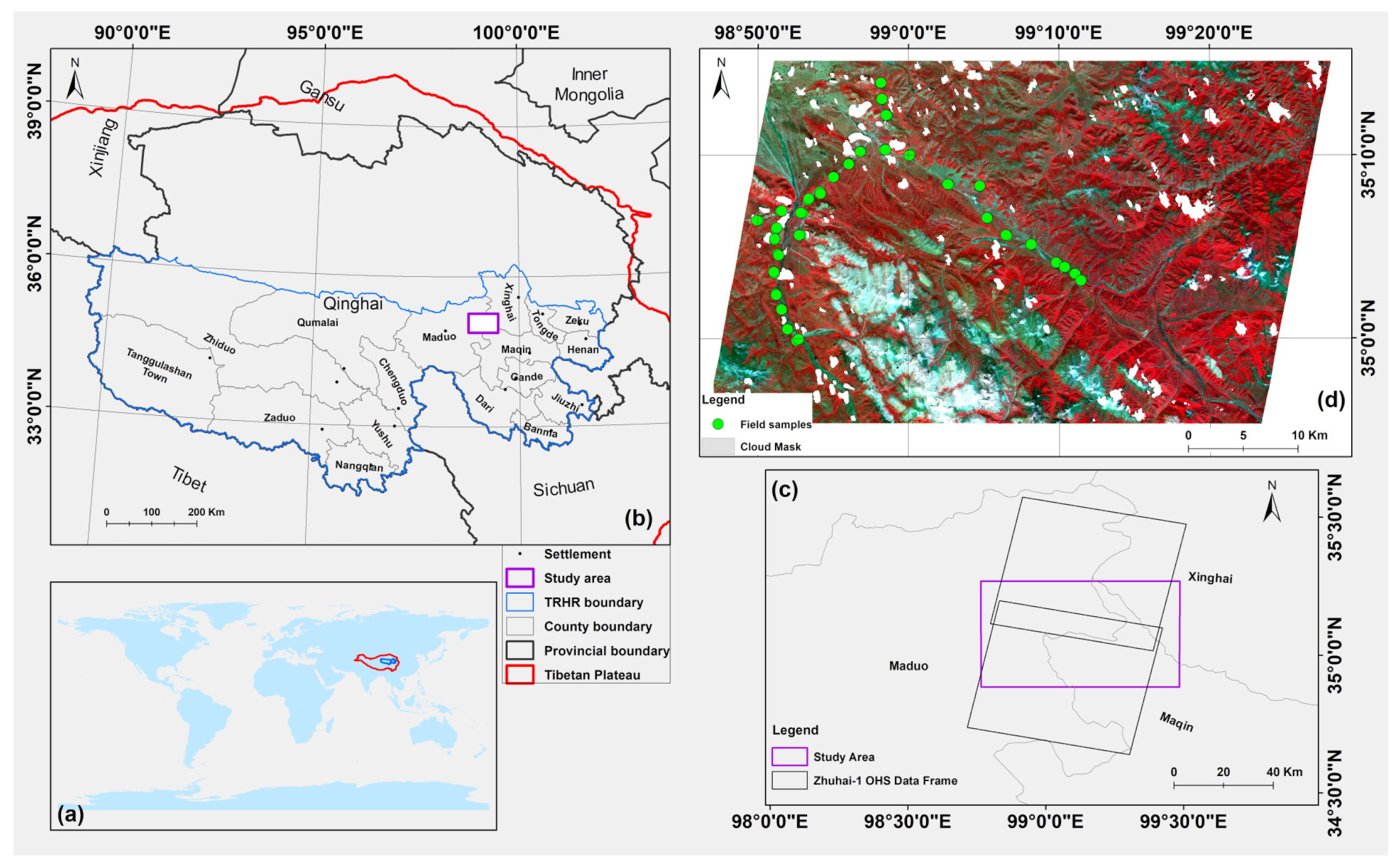
2. Study Area
3. Materials and Methods
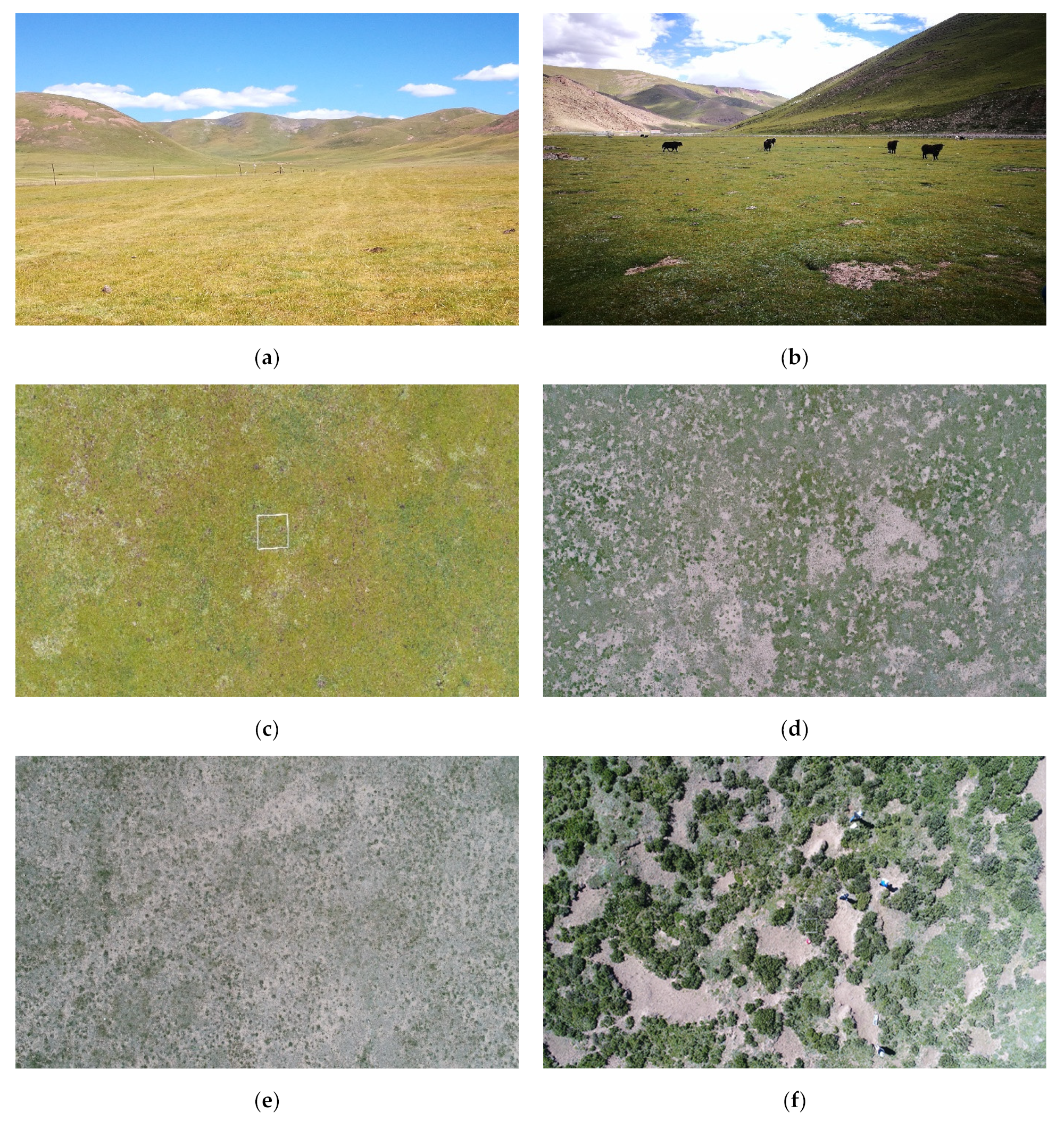
3.1. In-Situ Grassland Coverage Collection
3.2. Remote Sensing Imagery Acquisition and Data Processing
3.3. Land Use/Cover Datasets
3.4. MESMA Method Procedure
3.5. Accuracy Assessment
3.6. RMSE Distribution Analysis
4. Results
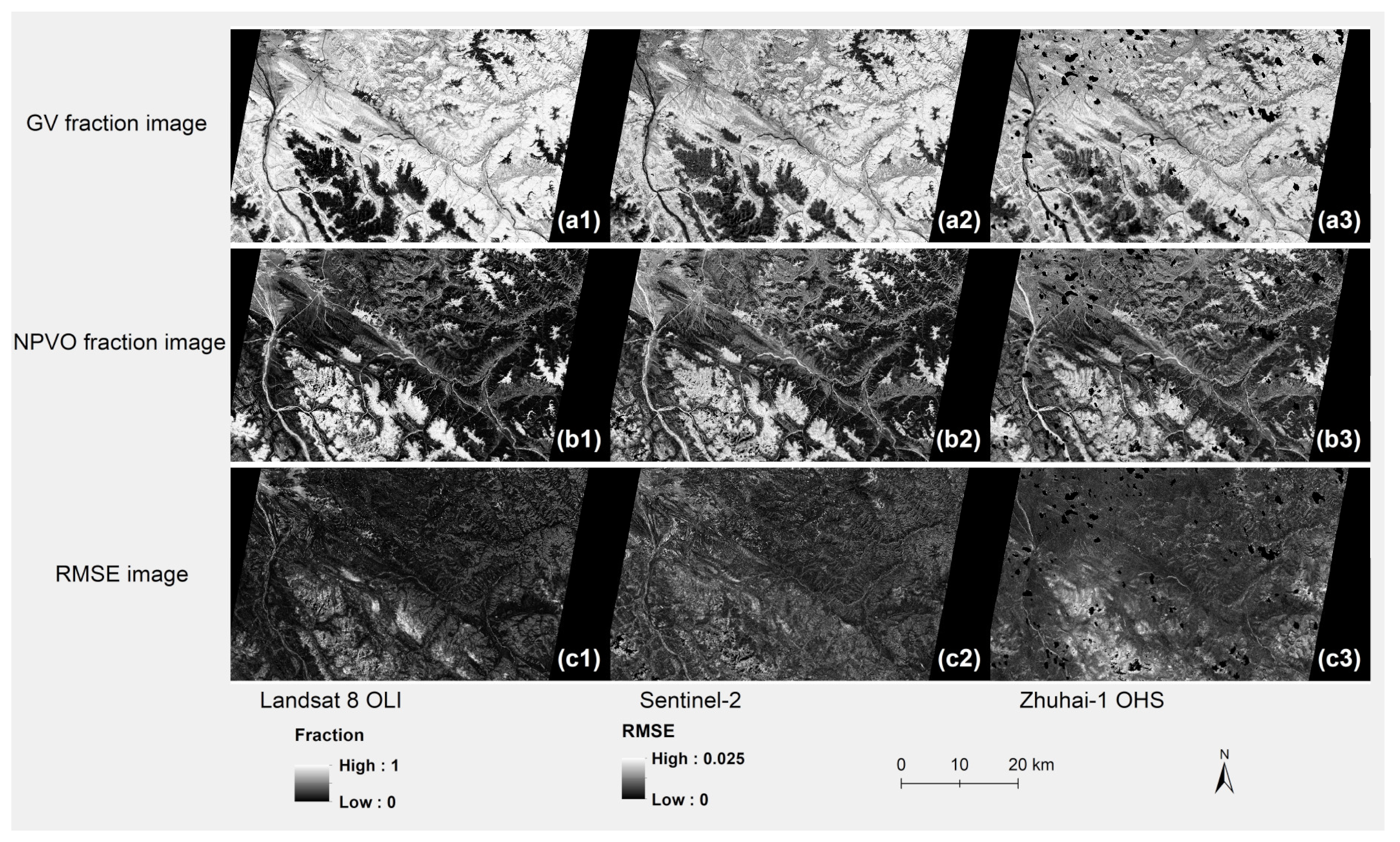
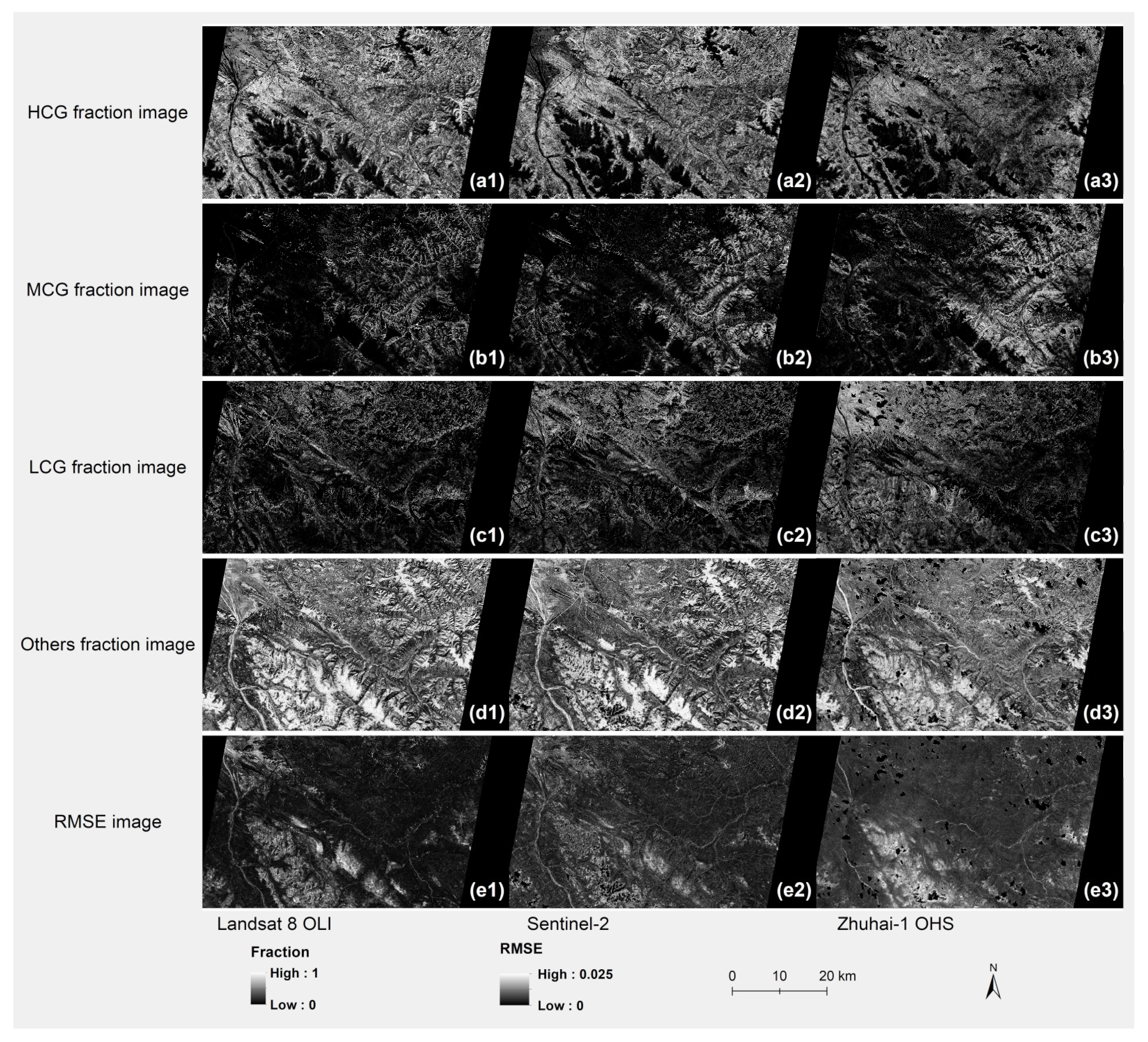
4.1. MESMA Classification
4.2. Endmember Spectral Libraries
4.3. MESMA Classification Accuracy
5. Discussion
5.1. MESMA Endmember Selection and Model Performance
5.2. RMSE Distribution
6. Conclusions
Supplementary Materials
Author Contributions
Funding
Data Availability Statement
Acknowledgments
Conflicts of Interest
References
- An, R.; Zhang, C.; Sun, M.; Wang, H.; Shen, X.; Wang, B.; Xing, F.; Huang, X.; Fan, M. Monitoring grassland degradation and restoration using a novel climate use efficiency (NCUE) index in the Tibetan Plateau, China. Ecol. Indic. 2021, 131, 108208. [Google Scholar] [CrossRef]
- Scurlock, J.M.O.; Hall, D.O. The global carbon sink: A grassland perspective. Glob. Chang. Biol. 1998, 4, 229–233. [Google Scholar] [CrossRef]
- Xu, D.; Guo, X.; Li, Z.; Yang, X.; Yin, H. Measuring the dead component of mixed grassland with Landsat imagery. Remote Sens. Environ. 2014, 142, 33–43. [Google Scholar] [CrossRef]
- Bardgett, R.D.; Bullock, J.M.; Lavorel, S.; Manning, P.; Schaffner, U.; Ostle, N.; Chomel, M.; Durigan, G.; Fry, E.L.; Johnson, D.; et al. Combatting global grassland degradation. Nat. Rev. Earth Environ. 2021, 2, 720–735. [Google Scholar] [CrossRef]
- Piipponen, J.; Jalava, M.; de Leeuw, J.; Rizayeva, A.; Godde, C.; Herrero, M.; Kummu, M. Global assessment of grassland carrying capacities and relative stocking densities of livestock. Glob. Chang. Biol. 2022, 28, 3902–3919. [Google Scholar] [CrossRef]
- Török, P.; Brudvig, L.A.; Kollmann, J.; Price, J.; Tóthmérész, B. The present and future of grassland restoration. Restor. Ecol. 2021, 29, e13378. [Google Scholar] [CrossRef]
- Lehnert, L.W.; Meyer, H.; Wang, Y.; Miehe, G.; Thies, B.; Reudenbach, C.; Bendix, J. Retrieval of grassland plant coverage on the Tibetan Plateau based on a multi-scale, multi-sensor and multi-method approach. Remote Sens. Environ. 2015, 164, 197–207. [Google Scholar] [CrossRef]
- Piao, S.; Ciais, P.; Huang, Y.; Shen, Z.; Peng, S.; Li, J.; Zhou, L.; Liu, H.; Ma, Y.; Ding, Y.; et al. The impacts of climate change on water resources and agriculture in China. Nature 2010, 467, 43–51. [Google Scholar] [CrossRef]
- Fassnacht, F.E.; Li, L.; Fritz, A. Mapping degraded grassland on the Eastern Tibetan Plateau with multi-temporal Landsat 8 data—Where do the severely degraded areas occur? Int. J. Appl. Earth Obs. Geoinf. 2015, 42, 115–127. [Google Scholar] [CrossRef]
- Wang, W.; Wang, Q.; Wang, H. The effect of land management on plant community composition, species diversity, and productivity of alpine Kobersia steppe meadow. Ecol. Res. 2005, 21, 181–187. [Google Scholar] [CrossRef]
- Cao, J.; Adamowski, J.F.; Deo, R.C.; Xu, X.; Gong, Y.; Feng, Q. Grassland degradation on the Qinghai-Tibetan Plateau: Reevaluation of causative factors. Rangel. Ecol. Manag. 2019, 72, 988–995. [Google Scholar] [CrossRef]
- Li, C.; de Jong, R.; Schmid, B.; Wulf, H.; Schaepman, M.E. Changes in grassland cover and in its spatial heterogeneity indicate degradation on the Qinghai-Tibetan Plateau. Ecol. Indic. 2020, 119, 106641. [Google Scholar] [CrossRef]
- Li, B. The rangeland degradation in North China and its preventive strategy. Sci. Agric. Sin. 1997, 30, 1–9. [Google Scholar]
- Purevdorj, T.S.; Tateishi, R.; Ishiyama, T.; Honda, Y. Relationships between percent vegetation cover and vegetation indices. Int. J. Remote Sens. 1998, 19, 3519–3535. [Google Scholar] [CrossRef]
- Xing, F.; An, R.; Wang, B.; Miao, J.; Jiang, T.; Huang, X.; Hu, Y. Mapping the occurrence and spatial distribution of noxious weed species with multisource data in degraded grasslands in the Three-River Headwaters Region, China. Sci. Total Environ. 2021, 801, 149714. [Google Scholar] [CrossRef] [PubMed]
- Gao, Q.; Wan, Y.; Xu, H.; Li, Y.; Jiangcun, W.; Borjigidai, A. Alpine grassland degradation index and its response to recent climate variability in Northern Tibet, China. Quat. Int. 2010, 226, 143–150. [Google Scholar] [CrossRef]
- Ge, J.; Meng, B.; Liang, T.; Feng, Q.; Gao, J.; Yang, S.; Huang, X.; Xie, H. Modeling alpine grassland cover based on MODIS data and support vector machine regression in the headwater region of the Huanghe River, China. Remote Sens. Environ. 2018, 218, 162–173. [Google Scholar] [CrossRef]
- Yagoub, H.; Belbachir, A.H.; Benabadji, N. Detection and mapping vegetation cover based on the Spectral Angle Mapper algorithm using NOAA AVHRR data. Adv. Space Res. 2014, 53, 1686–1693. [Google Scholar] [CrossRef]
- Dennison, P.E.; Qi, Y.; Meerdink, S.K.; Kokaly, R.F.; Thompson, D.R.; Daughtry, C.S.T.; Quemada, M.; Roberts, D.A.; Gader, P.D.; Wetherley, E.B.; et al. Comparison of methods for modeling fractional cover using simulated satellite hyperspectral imager spectra. Remote Sens. 2019, 11, 2072. [Google Scholar] [CrossRef]
- Tuia, D.; Verrelst, J.; Alonso, L.; Perez-Cruz, F.; Camps-Valls, G. Multioutput support vector regression for remote sensing biophysical parameter estimation. IEEE Geosci. Remote Sens. Lett. 2011, 8, 804–808. [Google Scholar] [CrossRef]
- Verrelst, J.; Muñoz, J.; Alonso, L.; Delegido, J.; Rivera, J.P.; Camps-Valls, G.; Moreno, J. Machine learning regression algorithms for biophysical parameter retrieval: Opportunities for Sentinel-2 and -3. Remote Sens. Environ. 2012, 118, 127–139. [Google Scholar] [CrossRef]
- Schwieder, M.; Leitao, P.J.; Suess, S.; Senf, C.; Hostert, P. Estimating fractional shrub cover using simulated EnMAP data: A comparison of three machine learning regression techniques. Remote Sens. 2014, 6, 3427–3445. [Google Scholar] [CrossRef]
- Fernandez-Manso, A.; Quintano, C.; Roberts, D.A. Burn severity influence on post-fire vegetation cover resilience from Landsat MESMA fraction images time series in Mediterranean forest ecosystems. Remote Sens. Environ. 2016, 184, 112–123. [Google Scholar] [CrossRef]
- Roberts, D.A.; Dennison, P.E.; Roth, K.L.; Dudley, K.; Hulley, G. Relationships between dominant plant species, fractional cover and Land Surface Temperature in a Mediterranean ecosystem. Remote Sens. Environ. 2015, 167, 152–167. [Google Scholar] [CrossRef]
- Roberts, D.A.; Gardner, M.; Church, R.; Ustin, S.; Scheer, G.; Green, R.O. Mapping chaparral in the Santa Monica Mountains using multiple endmember spectral mixture models. Remote Sens. Environ. 1998, 65, 267–279. [Google Scholar] [CrossRef]
- Wang, B.; An, R.; Zhang, Y.; Ai, Z. Mapping of Native Plant Species and Noxious Weeds in Typical Area of the Three-River Headwaters Region by Using Worldview-2 Imagery. In Image and Graphics; Springer: Berlin/Heidelberg, Germany, 2019; pp. 320–333. [Google Scholar] [CrossRef]
- Wang, D.; Qiu, P.; Wan, B.; Cao, Z.; Zhang, Q. Mapping α- and β-diversity of mangrove forests with multispectral and hyperspectral images. Remote Sens. Environ. 2022, 275, 113021. [Google Scholar] [CrossRef]
- Zhuhai Orbita Aerospace Science and Technology Co., Ltd. “Zhuhai-1" Hyperspectral Satellite Data Products User Handbook_V2.5; Zhuhai Orbita Aerospace Science and Technology Co., Ltd.: Zhuhai, China, 2021. (In Chinese) [Google Scholar]
- Cao, L.; Zhang, D.; Guo, Q.; Zhan, J. Inversion of Water Quality Parameter bod5 Based on Hyperspectral Remotely Sensed Data in Qinghai Lake. In Proceedings of the 2021 IEEE International Geoscience and Remote Sensing Symposium IGARSS, Brussels, Belgium, 11–16 July 2021. [Google Scholar]
- Mo, Y.; Zhong, R.F.; Cao, S.S. Orbita hyperspectral satellite image for land cover classification using random forest classifier. J. Appl. Remote Sens. 2021, 15, 014519. [Google Scholar] [CrossRef]
- Fu, B.; Liu, M.; He, H.; Lan, F.; He, X.; Liu, L.; Huang, L.; Fan, D.; Zhao, M.; Jia, Z. Comparison of optimized object-based RF-DT algorithm and SegNet algorithm for classifying Karst wetland vegetation communities using ultra-high spatial resolution UAV data. Int. J. Appl. Earth Obs. Geoinf. 2021, 104, 102553. [Google Scholar] [CrossRef]
- Wang, S.; Li, S.; Zheng, S.; Gao, W.; Zhang, Y.; Cao, B.; Cui, B.; Shao, D. Estimating biomass and carbon sequestration capacity of phragmites australis using remote sensing and growth dynamics modeling: A case study in Beijing hanshiqiao wetland nature reserve, China. Sensors 2022, 22, 3141. [Google Scholar] [CrossRef] [PubMed]
- Kahaer, Y.; Tashpolat, N.; Shi, Q.; Liu, S. Possibility of Zhuhai-1 hyperspectral imagery for monitoring salinized soil moisture content using fractional order differentially optimized spectral indices. Water 2020, 12, 3360. [Google Scholar] [CrossRef]
- Sheng, W.; Zhen, L.; Xiao, Y.; Hu, Y. Ecological and socioeconomic effects of ecological restoration in China’s Three Rivers Source Region. Sci. Total Environ. 2019, 650, 2307–2313. [Google Scholar] [CrossRef] [PubMed]
- Xiong, Q.; Xiao, Y.; Halmy, M.W.A.; Dakhil, M.A.; Liang, P.; Liu, C.; Zhang, L.; Pandey, B.; Pan, K.; El Kafraway, S.B.; et al. Monitoring the impact of climate change and human activities on grassland vegetation dynamics in the northeastern Qinghai-Tibet Plateau of China during 2000–2015. J. Arid Land 2019, 11, 637–651. [Google Scholar] [CrossRef]
- Liu, J.; Xu, X.; Shao, Q. Grassland degradation in the “Three-River Headwaters” region, Qinghai Province. J. Geogr. Sci. 2008, 18, 259–273. [Google Scholar] [CrossRef]
- Station Q.R.W. Grassland Resources of Qinghai; Qinghai People’s Publish Press Co., Ltd.: Xining, China, 2012. [Google Scholar]
- Liya Wang, H.K. Grassland Resources and the Dominated Plants Atlas of Sanjiangyuan Region; Qinghai People’s Publish Press: Xining, China, 2011. [Google Scholar]
- Pan, D. Study on the Types and Grade Partition Criterion of Black Soil Type Degraded Grassland in the Three-River Headwaters Region; Gansu Agricultural University: Lanzhou, China, 2007. [Google Scholar]
- Liu, J.; Xu, X.; Shao, Q. The spatial and temporal characteristics of grassland degradation in the Three-River Headwaters Region in Qinghai Province. Acta Geogr. Scnica 2008, 63, 364–376. [Google Scholar]
- Dorji, T.; Totland, Ø.; Moe, S.R. Are droppings, distance from pastoralist camps, and Pika burrows good proxies for local grazing pressure? Rangel. Ecol. Manag. 2013, 66, 26–33. [Google Scholar] [CrossRef]
- Cliff, A.D.; Ord, J.K. Spatial Autocorrelation; Pion Limited: London, UK, 1973; p. 178. [Google Scholar]
- Congalton, R.G. A review of assessing the accuracy of classification of remotely sensed data. Remote Sens. Environ. 1991, 37, 35–46. [Google Scholar] [CrossRef]
- Congalton, R.G. Using spatial autocorrelation analysis to explore the errors in maps generated from remotely sensed data. Photogramm. Eng. Remote Sens. 1988, 5, 587–592. [Google Scholar]
- Zhuhai Orbita Aerospace Science and Technology Co., Ltd. “Zhuhai-1” OHS Hyperspectral Data Pre-Processing Handbook_V1.2; Zhuhai Orbita Aerospace Science and Technology Co., Ltd.: Zhuhai, China, 2021. (In Chinese) [Google Scholar]
- Gao, Y.; Zhang, W. A simple empirical topographic correction method for ETM+ imagery. Int. J. Remote Sens. 2009, 30, 2259–2275. [Google Scholar] [CrossRef]
- Teillet, P.M.; Guindon, B.; Goodenough, D.G. On the slope-aspect correction of multispectral scanner data. Can. J. Remote Sens. 2014, 8, 84–106. [Google Scholar] [CrossRef]
- Yao, M.; Huang, J.; Zhang, M.; Zhou, H.; Kuang, L.; Ye, F. A comprehensive evaluation method for topographic correction model of remote sensing image based on entropy weight method. Open Geosci. 2022, 14, 354–366. [Google Scholar] [CrossRef]
- Xu, X.; Liu, J.; Zhang, S.; Li, R.; Yan, C.; Wu, S. China’s Multi-Period Land Use Land Cover Remote Sensing Monitoring Data Set (CNLUCC); Data Registration and Publishing System of Resource and Environmental Science Data Cloud Platform; Chinese Academy of Sciences: Beijing, China, 2018. Available online: http://www.resdc.cn (accessed on 16 February 2023).
- Zanaga, D.; Van De Kerchove, R.; De Keersmaecker, W.; Souverijns, N.; Brockmann, C.; Quast, R.; Wevers, J.; Grosu, A.; Paccini, A.; Vergnaud, S.; et al. ESA WorldCover 10 m 2020 v100. 2021. Available online: https://zenodo.org/record/5571936#.ZEh4xM5ByUk (accessed on 16 February 2023).
- ESA. WorldCover Product User Manual 1.0. European Space Agency. Available online: https://esa-worldcover.org/en (accessed on 16 February 2023).
- Quintano, C.; Fernández-Manso, A.; Roberts, D.A. Enhanced burn severity estimation using fine resolution ET and MESMA fraction images with machine learning algorithm. Remote Sens. Environ. 2020, 244, 111815. [Google Scholar] [CrossRef]
- Quintano, C.; Fernandez-Manso, A.; Roberts, D.A. Burn severity mapping from Landsat MESMA fraction images and Land Surface Temperature. Remote Sens. Environ. 2017, 190, 83–95. [Google Scholar] [CrossRef]
- Roberts, D.A.; Halligan, K.; Dennison, P.; Dudley, K.; Somers, B.; Crabbé, A. VIPER Tools User Mannual Version 2.1; UCSB VIPER LAB: Santa Barbara, CA, USA, 2019. [Google Scholar]
- Dennison, P.E.; Roberts, D.A. The effects of vegetation phenology on endmember selection and species mapping in southern California chaparral. Remote Sens. Environ. 2003, 87, 295–309. [Google Scholar] [CrossRef]
- Dennison, P.E.; Halligan, K.Q.; Roberts, D.A. A comparison of error metrics and constraints for multiple endmember spectral mixture analysis and spectral angle mapper. Remote Sens. Environ. 2004, 93, 359–367. [Google Scholar] [CrossRef]
- Roberts, D.A.; Dennison, P.E.; Gardner, M.E.; Hetzel, Y.; Ustin, S.L.; Lee, C.T. Evaluation of the potential of hyperion for fire danger assessment by comparison to the airborne visible/infrared imaging spectrometer. IEEE Trans. Geosci. Remote Sens. 2003, 41, 1297–1310. [Google Scholar] [CrossRef]
- Congalton, R.G.; Green, K. Assessing the Accuracy of Remotely Sensed Data: Principles and Practices, 3rd ed.; CRC Press: Boca Raton, FL, USA, 2019. [Google Scholar]
- Quintano, C.; Fernández-Manso, A.; Roberts, D.A. Multiple Endmember Spectral Mixture Analysis (MESMA) to map burn severity levels from Landsat images in Mediterranean countries. Remote Sens. Environ. 2013, 136, 76–88. [Google Scholar] [CrossRef]
- Roth, K.L.; Roberts, D.A.; Dennison, P.E.; Alonzo, M.; Peterson, S.H.; Beland, M. Differentiating plant species within and across diverse ecosystems with imaging spectroscopy. Remote Sens. Environ. 2015, 167, 135–151. [Google Scholar] [CrossRef]
- Clark, M.L. Comparison of simulated hyperspectral HyspIRI and multispectral Landsat 8 and Sentinel-2 imagery for multi-seasonal, regional land-cover mapping. Remote Sens. Environ. 2017, 200, 311–325. [Google Scholar] [CrossRef]
- Ma, Z.; Redmond, R.L. Tau coefficients for accuracy assessment of classification of remote senisng data. Photogramm. Eng. Remote Sens. 1995, 61, 435–439. [Google Scholar]
- Powell, R.; Roberts, D.; Dennison, P.; Hess, L. Sub-pixel mapping of urban land cover using multiple endmember spectral mixture analysis: Manaus, Brazil. Remote Sens. Environ. 2007, 106, 253–267. [Google Scholar] [CrossRef]
- Wang, J.J.; Zhang, Y.; Bussink, C. Unsupervised multiple endmember spectral mixture analysis-based detection of opium poppy fields from an EO-1 Hyperion image in Helmand, Afghanistan. Sci. Total Environ. 2014, 476–477, 1–6. [Google Scholar] [CrossRef] [PubMed]
- Maselli, F. Multiclass spectral decomposition of remotely sensed scenes by selective pixel unmixing. IEEE Trans. Geosci. Remote Sens. 1998, 36, 1809–1820. [Google Scholar] [CrossRef]
- Fernandez-Manso, A.; Quintano, C.; Roberts, D.A. Burn severity analysis in Mediterranean forests using maximum entropy model trained with EO-1 Hyperion and LiDAR data. ISPRS J. Photogramm. Remote Sens. 2019, 155, 102–118. [Google Scholar] [CrossRef]
- Franke, J.; Roberts, D.A.; Halligan, K.; Menz, G. Hierarchical Multiple Endmember Spectral Mixture Analysis (MESMA) of hyperspectral imagery for urban environments. Remote Sens. Environ. 2009, 113, 1712–1723. [Google Scholar] [CrossRef]
- Lewis, S.A.; Hudak, A.T.; Robichaud, P.R.; Morgan, P.; Satterberg, K.L.; Strand, E.K.; Smith, A.M.S.; Zamudio, J.A.; Lentile, L.B. Indicators of burn severity at extended temporal scales: A decade of ecosystem response in mixed-conifer forests of western Montana. Int. J. Wildland Fire 2017, 26, 755–771. [Google Scholar] [CrossRef]
- Powell, R.L.; Roberts, D.A. Characterizing variability of the urban physical environment for a suite of cities in Rondônia, Brazil. Earth Interact. 2008, 12, 1–32. [Google Scholar] [CrossRef]
- Chen, F.; Wang, K.; Tang, T.F. Spectral unmixing using a sparse multiple-endmember spectral mixture model. IEEE Trans. Geosci. Remote Sens. 2016, 54, 5846–5861. [Google Scholar] [CrossRef]
- Okujeni, A.; van der Linden, S.; Tits, L.; Somers, B.; Hostert, P. Support vector regression and synthetically mixed training data for quantifying urban land cover. Remote Sens. Environ. 2013, 137, 184–197. [Google Scholar] [CrossRef]
- Brown, M.I.; Pearce, T.; Leon, J.; Sidle, R.; Wilson, R. Using remote sensing and traditional ecological knowledge (TEK) to understand mangrove change on the Maroochy River, Queensland, Australia. Appl. Geogr. 2018, 94, 71–83. [Google Scholar] [CrossRef]
- Ai, Z.T.; An, R.; Chen, Y.H.; Huang, L.J. Comparison of hyperspectral HJ-1A/HSI and multispectral Landsat 8 and Sentinel-2A imagery for estimating alpine grassland coverage in the Three-River Headwaters region. J. Appl. Remote Sens. 2019, 13, 014504. [Google Scholar] [CrossRef]
- Szabó, G.; Singh, S.K.; Szabó, S. Slope angle and aspect as influencing factors on the accuracy of the SRTM and the ASTER GDEM databases. Phys. Chem. Earth Parts A/B/C 2015, 83–84, 137–145. [Google Scholar] [CrossRef]
- Mukherjee, S.; Joshi, P.K.; Mukherjee, S.; Ghosh, A.; Garg, R.D.; Mukhopadhyay, A. Evaluation of vertical accuracy of open source Digital Elevation Model (DEM). Int. J. Appl. Earth Obs. Geoinf. 2013, 21, 205–217. [Google Scholar] [CrossRef]
- Tachikawa, T.; Kaku, M.; Iwasaki, A.; Gesch, D.B.; Oimoen, M.J.; Zhang, Z.; Danielson, J.J.; Krieger, T.; Curtis, B.; Haase, J.; et al. ASTER Global Digital Elevation Model Version 2—Summary of Validation Results; United States Geological Survey: Rishton, VA, USA, 2011; p. 27. [Google Scholar]
- Farr, T.G.; Rosen, P.A.; Caro, E.; Crippen, R.; Duren, R.; Hensley, S.; Kobrick, M.; Paller, M.; Rodriguez, E.; Roth, L.; et al. The shuttle radar topography mission. Rev. Geophys. 2007, 45, 1–33. [Google Scholar] [CrossRef]
- Rexer, M.; Hirt, C. Comparison of free high resolution digital elevation data sets (ASTER GDEM2, SRTM v2.1/v4.1) and validation against accurate heights from the Australian National Gravity Database. Aust. J. Earth Sci. 2014, 61, 213–226. [Google Scholar] [CrossRef]
- Forkuor, G.; Maathuis, B. Comparison of SRTM and ASTER Derived Digital Elevation Models over Two Regions in Ghana-Implications for Hydrological and Environmental Modeling; INTECH Open Access Publisher London: London, UK, 2012. [Google Scholar]
- Carabajal, C.C.; Harding, D.J. ICESat validation of SRTM C-band digital elevation models. Geophys. Res. Lett. 2005, 32, 1–5. [Google Scholar] [CrossRef]
- Pasolli, E.; Melgani, F.; Alajlan, N.; Conci, N. Optical image classification: A ground-truth design framework. IEEE Trans. Geosci. Remote Sens. 2012, 51, 3580–3597. [Google Scholar] [CrossRef]
- Li, S.; Hao, Q.; Gao, G.; Kang, X. The effect of ground truth on performance evaluation of hyperspectral image classification. IEEE Trans. Geosci. Remote Sens. 2018, 56, 7195–7206. [Google Scholar] [CrossRef]


| Cover Type | Dominant Species | Co-Occurring Species | Distributed Area | Elevation (m) | Proportion | References |
|---|---|---|---|---|---|---|
| Alpine meadows | Kobresia pygmaea, Kobresia humilis, Kobresia capillifolia | Herbarum variorum, Stipa aliena, Ptilagrostis spp. and Poa spp. | Southwest, central south, and east part of the TRHR | 3000~4800 | 72.15% | [37,38,39,40] |
| Alpine steppe | Stipa purpurea, Carex moorcroftii, Brylkinia caudata | Herbarum variorum, Poa spp. and Leymus secalinus | West and northwest of the TRHR | 3800~4600 | 21.44% |
| Data Sources | Acquisition Date | Bands | Spatial Resolution (m) | Spectral Resolution (nm) | Wavelength Region (nm) | Scenes |
|---|---|---|---|---|---|---|
| Landsat 8 OLI | 25 August 2020 | 7 | 30 | / | 450~880, 1570~2290 | 2 |
| Sentinel-2 | 17 September 2020 | 13 | 10 | / | 443~945, 1610~2190 | 4 |
| Zhuhai-1 OHS | 19 August 2020 | 32 | 10 | 2.5 | 400~1000 | 2 |
| Data Source | Spatial Resolution (m) | Year | Land Cover Types |
|---|---|---|---|
| CNLUCC | 30 | 2020 | Cultivated, forest, grassland (high-density grassland, medium-density grassland, low-density grassland), water, construction, and unused land |
| ESA WorldCover | 10 | 2020 | Tree cover, shrubland, grassland, cropland, built-up, bare/sparse vegetation, snow and ice, permanent water bodies, herbaceous wetland, mangroves, moss, and lichen |
| Model Complexity | Landsat 8 OLI | Sentinel-2 | Zhuhai-1 OHS |
|---|---|---|---|
| Number of pixels classified and the overall percentage (%) classified in each image at pixel scale | |||
| 2-EM | 98.9 | 97.2 | 98.5 |
| 8,995,210 | 19,888,207 | 19,501,999 | |
| 3-EM | 98.5 | 97.5 | 99.1 |
| 8,960,561 | 19,946,983 | 19,613,810 | |
| Number of pixels classified and the overall percentage (%) classified in each image at landscape scale | |||
| 2-EM models | 97.6 | 95.1 | 96.3 |
| 8,870,491 | 19,469,101 | 19,066,003 | |
| 3-EM models | 98.5 | 96.6 | 99.1 |
| 8,954,389 | 19,762,221 | 19,611,130 | |
| 4-EM models | 95.6 | 94.3 | 98.6 |
| 8,696,568 | 19,302,190 | 19,520,686 | |
| Accuracy Parameters | Landsat 8 OLI | Sentinel-2 | Zhuhai-1 OHS | |||
|---|---|---|---|---|---|---|
| GV | NPVO | GV | NPVO | GV | NPVO | |
| PA (%) | 91.1 | 90.9 | 85.5 | 96.8 | 92.1 | 93.1 |
| UA (%) | 97.3 | 73.8 | 99.0 | 65.0 | 98.0 | 76.6 |
| OA (%) | 91.1 | 88.0 | 92.3 | |||
| k-statistic | 0.76 | 0.70 | 0.79 | |||
| Zk-statistic | 20.8 | 17.9 | 23.6 | |||
| ZL8-S2-statistic | 0.7 | |||||
| ZL8-ZOHS-statistic | 0.7 | |||||
| ZS2-ZOHS-statistic | 1.86 | |||||
| Accuracy Parameters | Landsat 8 OLI | Sentinel-2 | Zhuhai-1 OHS | |||||||||
|---|---|---|---|---|---|---|---|---|---|---|---|---|
| HCG | MCG | LCG | Others | HCG | MCG | LCG | Others | HCG | MCG | LCG | Others | |
| PA (%) | 69.5 | 68.8 | 43.8 | 79.4 | 60.9 | 76.4 | 55.6 | 80.8 | 60.8 | 92.0 | 54.4 | 88.4 |
| UA (%) | 54.0 | 70.7 | 55.3 | 83.3 | 70.0 | 63.2 | 59.3 | 82.5 | 63.3 | 76.2 | 78.7 | 84.3 |
| OA (%) | 68.7 | 70.0 | 77.4 | |||||||||
| k-statistic | 0.57 | 0.60 | 0.69 | |||||||||
| Zk-test | 15.3 | 16.8 | 21.1 | |||||||||
| ZL8-S2-statistic | 0.5 | |||||||||||
| ZL8-ZOHS-statistic | 2.4 | |||||||||||
| ZS2-ZOHS-statistic | 1.92.3 | |||||||||||
Disclaimer/Publisher’s Note: The statements, opinions and data contained in all publications are solely those of the individual author(s) and contributor(s) and not of MDPI and/or the editor(s). MDPI and/or the editor(s) disclaim responsibility for any injury to people or property resulting from any ideas, methods, instructions or products referred to in the content. |
© 2023 by the authors. Licensee MDPI, Basel, Switzerland. This article is an open access article distributed under the terms and conditions of the Creative Commons Attribution (CC BY) license (https://creativecommons.org/licenses/by/4.0/).
Share and Cite
Xing, F.; An, R.; Guo, X.; Shen, X.; Soubry, I.; Wang, B.; Mu, Y.; Huang, X. Mapping Alpine Grassland Fraction Coverage Using Zhuhai-1 OHS Imagery in the Three River Headwaters Region, China. Remote Sens. 2023, 15, 2289. https://doi.org/10.3390/rs15092289
Xing F, An R, Guo X, Shen X, Soubry I, Wang B, Mu Y, Huang X. Mapping Alpine Grassland Fraction Coverage Using Zhuhai-1 OHS Imagery in the Three River Headwaters Region, China. Remote Sensing. 2023; 15(9):2289. https://doi.org/10.3390/rs15092289
Chicago/Turabian StyleXing, Fei, Ru An, Xulin Guo, Xiaoji Shen, Irini Soubry, Benlin Wang, Yanmei Mu, and Xianglin Huang. 2023. "Mapping Alpine Grassland Fraction Coverage Using Zhuhai-1 OHS Imagery in the Three River Headwaters Region, China" Remote Sensing 15, no. 9: 2289. https://doi.org/10.3390/rs15092289
APA StyleXing, F., An, R., Guo, X., Shen, X., Soubry, I., Wang, B., Mu, Y., & Huang, X. (2023). Mapping Alpine Grassland Fraction Coverage Using Zhuhai-1 OHS Imagery in the Three River Headwaters Region, China. Remote Sensing, 15(9), 2289. https://doi.org/10.3390/rs15092289