
Cropland Extraction in Southern China from Very High-Resolution Images Based on Deep Learning


Abstract
1. Introduction
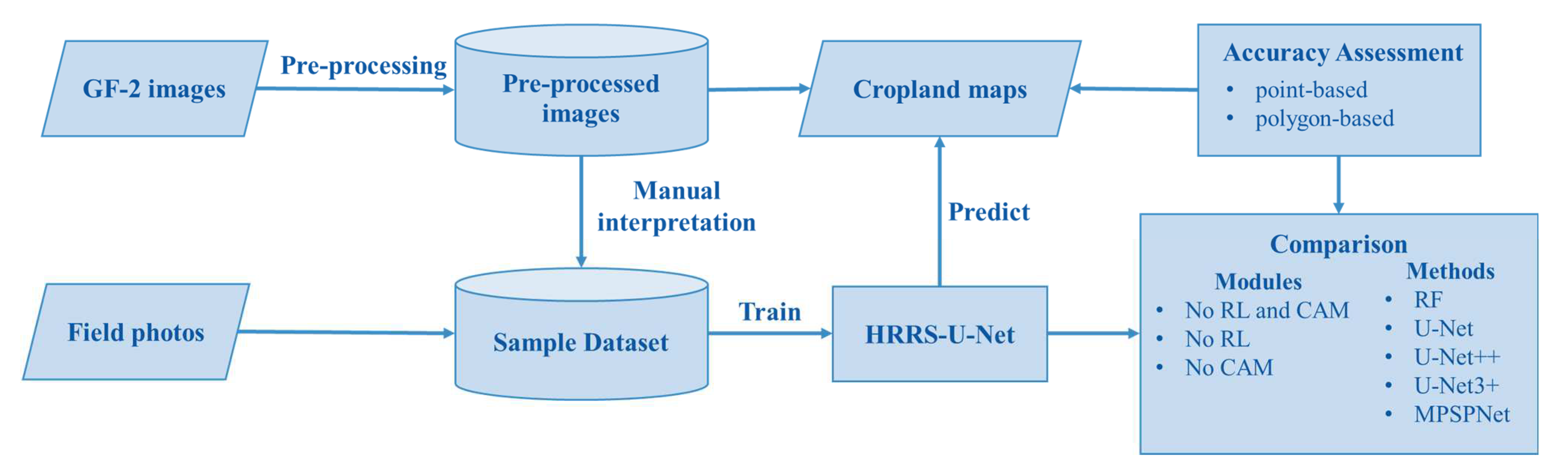
2. Methodology
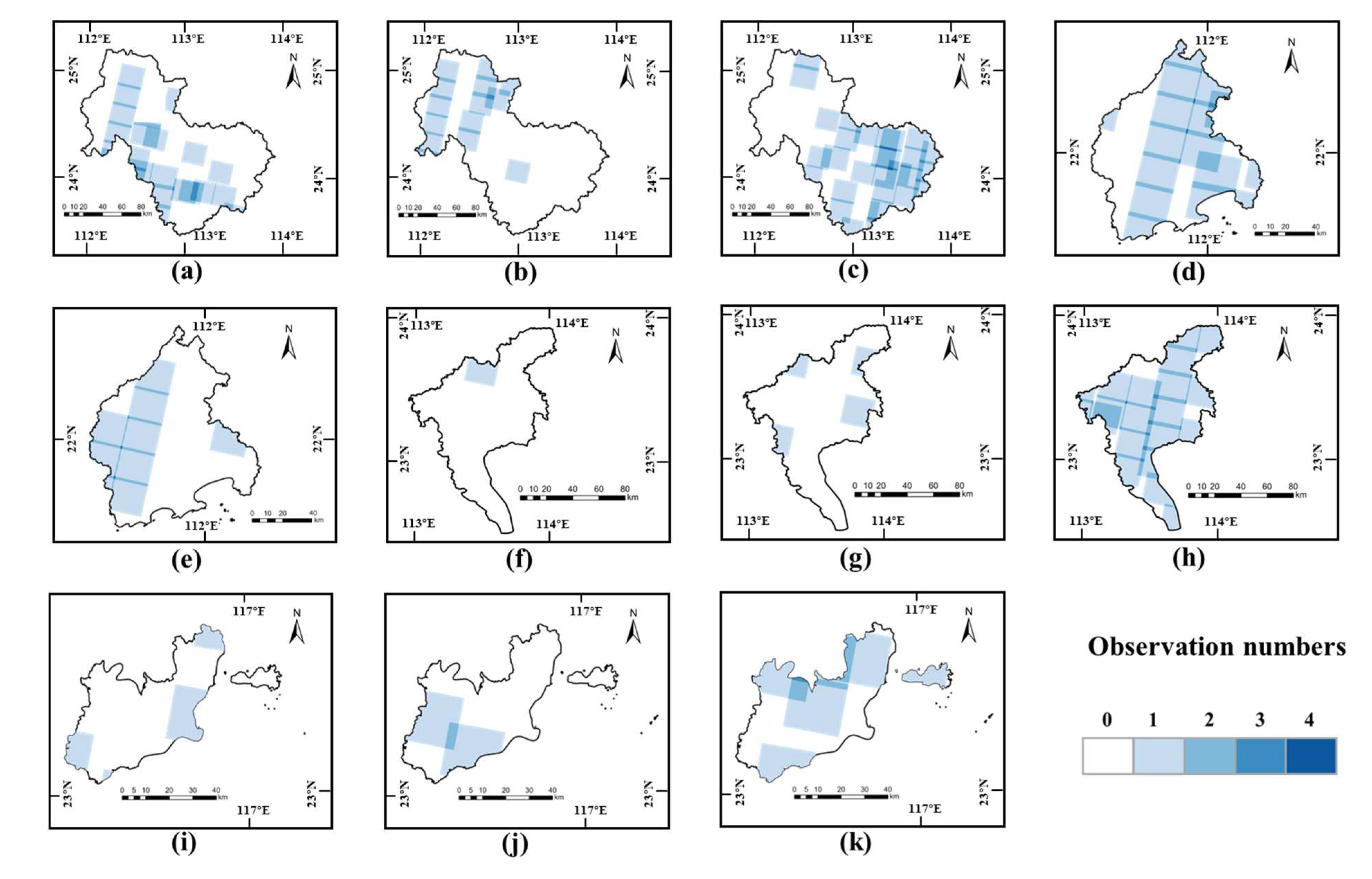
2.1. Study Area
2.2. Dataset
2.2.1. Data Sources and Pre-Processing
2.2.2. Sample Dataset
2.3. Deep Learning Model
2.3.1. Parallel Convolutional Module Streams
2.3.2. Multi-Resolution Fusion
2.3.3. RS-Block
2.4. Model Training
2.5. Accuracy Assessment
3. Results
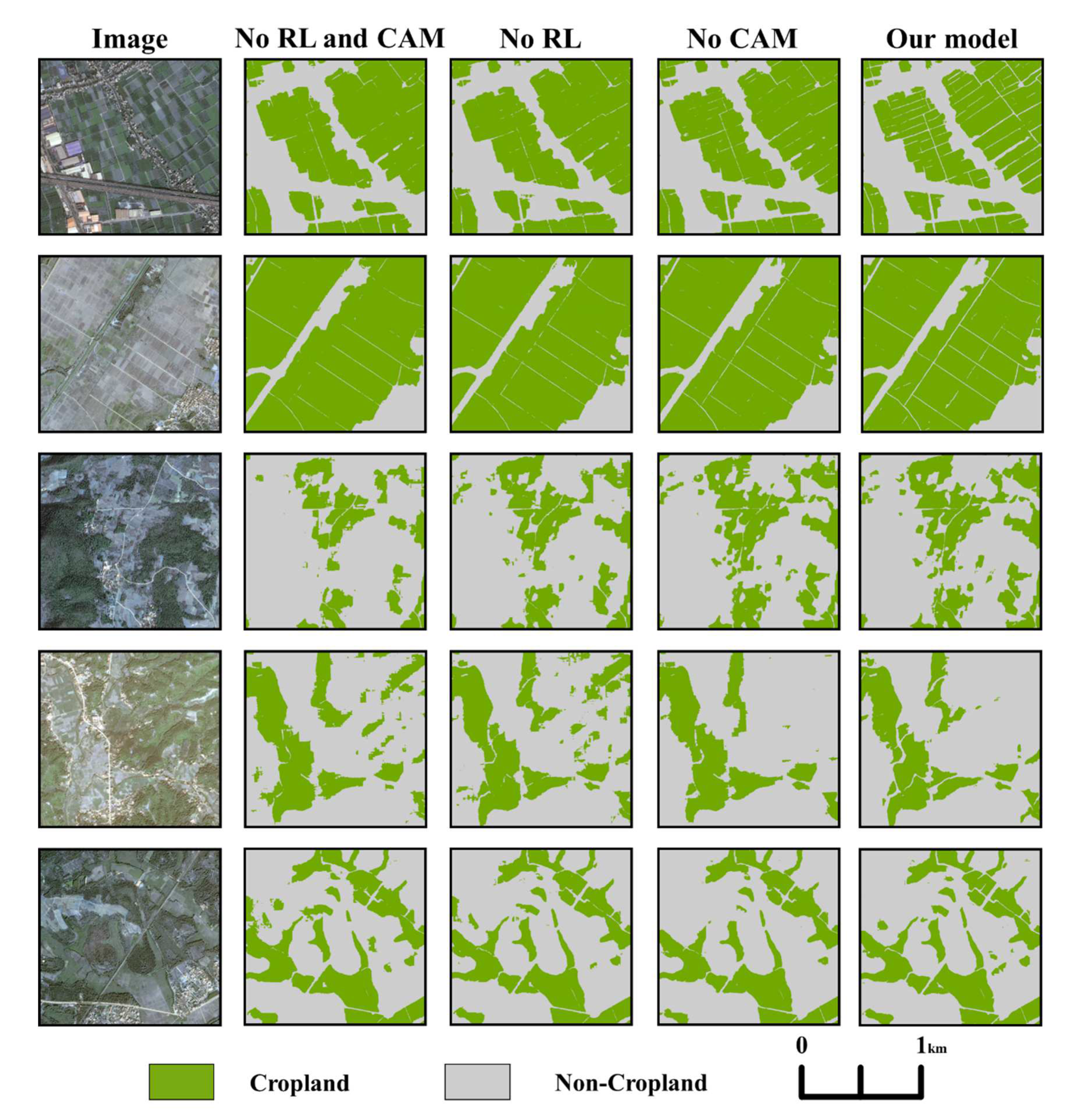
3.1. Ablation Experiment Results of the RS-Block
3.2. Comparison of HRRS-U-Net with Other Methods
3.3. Results of Cropland Extraction
4. Discussion
4.1. Maintaining High-Resolution Representation to Improve Boundary Delineation
4.2. Extracting Representative Features to Generalize Highly Spatio-Temporal Heterogeneous Cropland
4.3. Uncertainty Analysis
4.4. Implications and Future Work
5. Conclusions
Author Contributions
Funding
Data Availability Statement
Conflicts of Interest
References
- Liu, L.; Xiao, X.; Qin, Y.; Wang, J.; Xu, X.; Hu, Y.; Qiao, Z. Mapping Cropping Intensity in China Using Time Series Landsat and Sentinel-2 Images and Google Earth Engine. Remote Sens. Environ. 2020, 239, 111624. [Google Scholar] [CrossRef]
- Viana, C.M.; Freire, D.; Abrantes, P.; Rocha, J.; Pereira, P. Agricultural Land Systems Importance for Supporting Food Security and Sustainable Development Goals: A Systematic Review. Sci. Total Environ. 2022, 806, 150718. [Google Scholar] [CrossRef] [PubMed]
- Di, Y.; Zhang, G.; You, N.; Yang, T.; Zhang, Q.; Liu, R.; Doughty, R.B.; Zhang, Y. Mapping Croplands in the Granary of the Tibetan Plateau Using All Available Landsat Imagery, A Phenology-Based Approach, and Google Earth Engine. Remote Sens. 2021, 13, 2289. [Google Scholar] [CrossRef]
- Waldner, F.; Bellemans, N.; Hochman, Z.; Newby, T.; de Abelleyra, D.; Verón, S.R.; Bartalev, S.; Lavreniuk, M.; Kussul, N.; Maire, G.L.; et al. Roadside Collection of Training Data for Cropland Mapping Is Viable When Environmental and Management Gradients Are Surveyed. Int. J. Appl. Earth Obs. Geoinf. 2019, 80, 82–93. [Google Scholar] [CrossRef]
- Liu, J.; Liu, M.; Tian, H.; Zhuang, D.; Zhang, Z.; Zhang, W.; Tang, X.; Deng, X. Spatial and Temporal Patterns of China’s Cropland during 1990–2000: An Analysis Based on Landsat TM Data. Remote Sens. Environ. 2005, 98, 442–456. [Google Scholar] [CrossRef]
- Wang, X.; Yan, F.; Su, F. Impacts of Urbanization on the Ecosystem Services in the Guangdong-Hong Kong-Macao Greater Bay Area, China. Remote Sens. 2020, 12, 3269. [Google Scholar] [CrossRef]
- Liu, L.; Xu, X.; Liu, J.; Chen, X.; Ning, J. Impact of Farmland Changes on Production Potential in China during 1990–2010. J. Geogr. Sci. 2015, 25, 19–34. [Google Scholar] [CrossRef]
- Potapov, P.; Turubanova, S.; Hansen, M.C.; Tyukavina, A.; Zalles, V.; Khan, A.; Song, X.-P.; Pickens, A.; Shen, Q.; Cortez, J. Global Maps of Cropland Extent and Change Show Accelerated Cropland Expansion in the Twenty-First Century. Nat. Food 2022, 3, 19–28. [Google Scholar] [CrossRef]
- Fritz, S.; See, L.; McCallum, I.; You, L.; Bun, A.; Moltchanova, E.; Duerauer, M.; Albrecht, F.; Schill, C.; Perger, C.; et al. Mapping Global Cropland and Field Size. Glob. Change Biol. 2015, 21, 1980–1992. [Google Scholar] [CrossRef]
- Hao, P.; Löw, F.; Biradar, C. Annual Cropland Mapping Using Reference Landsat Time Series—A Case Study in Central Asia. Remote Sens. 2018, 10, 2057. [Google Scholar] [CrossRef]
- Oliphant, A.J.; Thenkabail, P.S.; Teluguntla, P.; Xiong, J.; Gumma, M.K.; Congalton, R.G.; Yadav, K. Mapping Cropland Extent of Southeast and Northeast Asia Using Multi-Year Time-Series Landsat 30-m Data Using a Random Forest Classifier on the Google Earth Engine Cloud. Int. J. Appl. Earth Obs. Geoinf. 2019, 81, 110–124. [Google Scholar] [CrossRef]
- Htitiou, A.; Boudhar, A.; Chehbouni, A.; Benabdelouahab, T. National-Scale Cropland Mapping Based on Phenological Metrics, Environmental Covariates, and Machine Learning on Google Earth Engine. Remote Sens. 2021, 13, 4378. [Google Scholar] [CrossRef]
- Bartholomé, E.; Belward, A.S. GLC2000: A New Approach to Global Land Cover Mapping from Earth Observation Data. Int. J. Remote Sens. 2005, 26, 1959–1977. [Google Scholar] [CrossRef]
- Friedl, M.; Sulla-Menashe, D. MCD12Q1 MODIS/Terra+Aqua Land Cover Type Yearly L3 Global 500m SIN Grid V006; NASA: Washington, DC, USA, 2019. [Google Scholar]
- Friedl, M.; Gray, J.; Sulla-Menashe, D. MCD12Q2 MODIS/Terra+Aqua Land Cover Dynamics Yearly L3 Global 500m SIN Grid V006; NASA: Washington, DC, USA, 2019. [Google Scholar]
- Buchhorn, M.; Lesiv, M.; Tsendbazar, N.-E.; Herold, M.; Bertels, L.; Smets, B. Copernicus Global Land Cover Layers—Collection 2. Remote Sens. 2020, 12, 1044. [Google Scholar] [CrossRef]
- Yu, L.; Wang, J.; Clinton, N.; Xin, Q.; Zhong, L.; Chen, Y.; Gong, P. FROM-GC: 30 m Global Cropland Extent Derived through Multisource Data Integration. Int. J. Digit. Earth 2013, 6, 521–533. [Google Scholar] [CrossRef]
- Yang, J.; Huang, X. The 30 m Annual Land Cover Dataset and Its Dynamics in China from 1990 to 2019. Earth Syst. Sci. Data 2021, 13, 3907–3925. [Google Scholar] [CrossRef]
- Brown, C.F.; Brumby, S.P.; Guzder-Williams, B.; Birch, T.; Hyde, S.B.; Mazzariello, J.; Czerwinski, W.; Pasquarella, V.J.; Haertel, R.; Ilyushchenko, S.; et al. Dynamic World, Near Real-Time Global 10 m Land Use Land Cover Mapping. Sci. Data 2022, 9, 251. [Google Scholar] [CrossRef]
- Panda, S.S.; Rao, M.N.; Thenkabail, P.; Fitzerald, J.E. Remote Sensing Systems—Platforms and Sensors: Aerial, Satellite, UAV, Optical, Radar, and LiDAR. In Remotely Sensed Data Characterization, Classification, and Accuracies; CRC Press: Boca Raton, FL, USA, 2015; ISBN 978-0-429-08939-8. [Google Scholar]
- Zhang, H.; Liu, M.; Wang, Y.; Shang, J.; Liu, X.; Li, B.; Song, A.; Li, Q. Automated Delineation of Agricultural Field Boundaries from Sentinel-2 Images Using Recurrent Residual U-Net. Int. J. Appl. Earth Obs. Geoinf. 2021, 105, 102557. [Google Scholar] [CrossRef]
- Yang, Y.; Xiao, P.; Feng, X.; Li, H. Accuracy Assessment of Seven Global Land Cover Datasets over China. ISPRS J. Photogramm. Remote Sens. 2017, 125, 156–173. [Google Scholar] [CrossRef]
- Zhang, C.; Dong, J.; Ge, Q. Quantifying the Accuracies of Six 30-m Cropland Datasets over China: A Comparison and Evaluation Analysis. Comput. Electron. Agric. 2022, 197, 106946. [Google Scholar] [CrossRef]
- Xiong, J.; Thenkabail, P.S.; Tilton, J.C.; Gumma, M.K.; Teluguntla, P.; Oliphant, A.; Congalton, R.G.; Yadav, K.; Gorelick, N. Nominal 30-m Cropland Extent Map of Continental Africa by Integrating Pixel-Based and Object-Based Algorithms Using Sentinel-2 and Landsat-8 Data on Google Earth Engine. Remote Sens. 2017, 9, 1065. [Google Scholar] [CrossRef]
- Zhang, D.; Pan, Y.; Zhang, J.; Hu, T.; Zhao, J.; Li, N.; Chen, Q. A Generalized Approach Based on Convolutional Neural Networks for Large Area Cropland Mapping at Very High Resolution. Remote Sens. Environ. 2020, 247, 111912. [Google Scholar] [CrossRef]
- Lu, R.; Wang, N.; Zhang, Y.; Lin, Y.; Wu, W.; Shi, Z. Extraction of Agricultural Fields via DASFNet with Dual Attention Mechanism and Multi-Scale Feature Fusion in South Xinjiang, China. Remote Sens. 2022, 14, 2253. [Google Scholar] [CrossRef]
- Xu, L.; Ming, D.; Zhou, W.; Bao, H.; Chen, Y.; Ling, X. Farmland Extraction from High Spatial Resolution Remote Sensing Images Based on Stratified Scale Pre-Estimation. Remote Sens. 2019, 11, 108. [Google Scholar] [CrossRef]
- Cai, Z.; Hu, Q.; Zhang, X.; Yang, J.; Wei, H.; He, Z.; Song, Q.; Wang, C.; Yin, G.; Xu, B. An Adaptive Image Segmentation Method with Automatic Selection of Optimal Scale for Extracting Cropland Parcels in Smallholder Farming Systems. Remote Sens. 2022, 14, 3067. [Google Scholar] [CrossRef]
- Liu, Z.; Li, N.; Wang, L.; Zhu, J.; Qin, F. A Multi-Angle Comprehensive Solution Based on Deep Learning to Extract Cultivated Land Information from High-Resolution Remote Sensing Images. Ecol. Indic. 2022, 141, 108961. [Google Scholar] [CrossRef]
- Li, S.; Song, W.; Fang, L.; Chen, Y.; Ghamisi, P.; Benediktsson, J.A. Deep Learning for Hyperspectral Image Classification: An Overview. IEEE Trans. Geosci. Remote Sens. 2019, 57, 6690–6709. [Google Scholar] [CrossRef]
- Rufin, P.; Bey, A.; Picoli, M.; Meyfroidt, P. Large-Area Mapping of Active Cropland and Short-Term Fallows in Smallholder Landscapes Using PlanetScope Data. Int. J. Appl. Earth Obs. Geoinf. 2022, 112, 102937. [Google Scholar] [CrossRef]
- Hu, Q.; Wu, W.; Song, Q.; Lu, M.; Chen, D.; Yu, Q.; Tang, H. How Do Temporal and Spectral Features Matter in Crop Classification in Heilongjiang Province, China? J. Integr. Agric. 2017, 16, 324–336. [Google Scholar] [CrossRef]
- Blickensdörfer, L.; Schwieder, M.; Pflugmacher, D.; Nendel, C.; Erasmi, S.; Hostert, P. Mapping of Crop Types and Crop Sequences with Combined Time Series of Sentinel-1, Sentinel-2 and Landsat 8 Data for Germany. Remote Sens. Environ. 2022, 269, 112831. [Google Scholar] [CrossRef]
- Samaniego, L.; Schulz, K. Supervised Classification of Agricultural Land Cover Using a Modified K-NN Technique (MNN) and Landsat Remote Sensing Imagery. Remote Sens. 2009, 1, 875–895. [Google Scholar] [CrossRef]
- Waldner, F.; Canto, G.S.; Defourny, P. Automated Annual Cropland Mapping Using Knowledge-Based Temporal Features. ISPRS J. Photogramm. Remote Sens. 2015, 110, 1–13. [Google Scholar] [CrossRef]
- Lin, L.; Di, L.; Zhang, C.; Guo, L.; Di, Y.; Li, H.; Yang, A. Validation and Refinement of Cropland Data Layer Using a Spatial-Temporal Decision Tree Algorithm. Sci. Data 2022, 9, 63. [Google Scholar] [CrossRef] [PubMed]
- Teluguntla, P.; Thenkabail, P.S.; Oliphant, A.; Xiong, J.; Gumma, M.K.; Congalton, R.G.; Yadav, K.; Huete, A. A 30-m Landsat-Derived Cropland Extent Product of Australia and China Using Random Forest Machine Learning Algorithm on Google Earth Engine Cloud Computing Platform. ISPRS J. Photogramm. Remote Sens. 2018, 144, 325–340. [Google Scholar] [CrossRef]
- Liu, R.; Tao, F.; Liu, X.; Na, J.; Leng, H.; Wu, J.; Zhou, T. RAANet: A Residual ASPP with Attention Framework for Semantic Segmentation of High-Resolution Remote Sensing Images. Remote Sens. 2022, 14, 3109. [Google Scholar] [CrossRef]
- Wang, M.; Wang, J.; Cui, Y.; Liu, J.; Chen, L. Agricultural Field Boundary Delineation with Satellite Image Segmentation for High-Resolution Crop Mapping: A Case Study of Rice Paddy. Agronomy 2022, 12, 2342. [Google Scholar] [CrossRef]
- Xiong, J.; Thenkabail, P.S.; Gumma, M.K.; Teluguntla, P.; Poehnelt, J.; Congalton, R.G.; Yadav, K.; Thau, D. Automated Cropland Mapping of Continental Africa Using Google Earth Engine Cloud Computing. ISPRS J. Photogramm. Remote Sens. 2017, 126, 225–244. [Google Scholar] [CrossRef]
- Dong, J.; Xiao, X.; Menarguez, M.A.; Zhang, G.; Qin, Y.; Thau, D.; Biradar, C.; Moore, B., III. Mapping Paddy Rice Planting Area in Northeastern Asia with Landsat 8 Images, Phenology-Based Algorithm and Google Earth Engine. Remote Sens. Environ. 2016, 185, 142–154. [Google Scholar] [CrossRef]
- Guo, Y.; Xia, H.; Pan, L.; Zhao, X.; Li, R.; Bian, X.; Wang, R.; Yu, C. Development of a New Phenology Algorithm for Fine Mapping of Cropping Intensity in Complex Planting Areas Using Sentinel-2 and Google Earth Engine. ISPRS Int. J. Geo-Inf. 2021, 10, 587. [Google Scholar] [CrossRef]
- Zheng, J.; Liu, L.; Chen, H.; Gou, Y.; Che, Y.; Xu, H.; Li, Q. Characteristics of Warm Clouds and Precipitation in South China during the Pre-Flood Season Using Datasets from a Cloud Radar, a Ceilometer, and a Disdrometer. Remote Sens. 2019, 11, 3045. [Google Scholar] [CrossRef]
- Zhang, L.; Zhang, L.; Du, B. Deep Learning for Remote Sensing Data: A Technical Tutorial on the State of the Art. IEEE Geosci. Remote Sens. Mag. 2016, 4, 22–40. [Google Scholar] [CrossRef]
- Kotaridis, I.; Lazaridou, M. Remote Sensing Image Segmentation Advances: A Meta-Analysis. ISPRS J. Photogramm. Remote Sens. 2021, 173, 309–322. [Google Scholar] [CrossRef]
- LeCun, Y.; Boser, B.; Denker, J.S.; Henderson, D.; Howard, R.E.; Hubbard, W.; Jackel, L.D. Backpropagation Applied to Handwritten Zip Code Recognition. Neural Comput. 1989, 1, 541–551. [Google Scholar] [CrossRef]
- Aminoff, E.M.; Baror, S.; Roginek, E.W.; Leeds, D.D. Contextual Associations Represented Both in Neural Networks and Human Behavior. Sci. Rep. 2022, 12, 5570. [Google Scholar] [CrossRef] [PubMed]
- Qing, Y.; Liu, W. Hyperspectral Image Classification Based on Multi-Scale Residual Network with Attention Mechanism. Remote Sens. 2021, 13, 335. [Google Scholar] [CrossRef]
- Xu, W.; Deng, X.; Guo, S.; Chen, J.; Sun, L.; Zheng, X.; Xiong, Y.; Shen, Y.; Wang, X. High-Resolution U-Net: Preserving Image Details for Cultivated Land Extraction. Sensors 2020, 20, 4064. [Google Scholar] [CrossRef]
- Shi, H.; Cao, G.; Zhang, Y.; Ge, Z.; Liu, Y.; Fu, P. H2A2Net: A Hybrid Convolution and Hybrid Resolution Network with Double Attention for Hyperspectral Image Classification. Remote Sens. 2022, 14, 4235. [Google Scholar] [CrossRef]
- Mei, X.; Pan, E.; Ma, Y.; Dai, X.; Huang, J.; Fan, F.; Du, Q.; Zheng, H.; Ma, J. Spectral-Spatial Attention Networks for Hyperspectral Image Classification. Remote Sens. 2019, 11, 963. [Google Scholar] [CrossRef]
- Wang, J.; Sun, K.; Cheng, T.; Jiang, B.; Deng, C.; Zhao, Y.; Liu, D.; Mu, Y.; Tan, M.; Wang, X.; et al. Deep High-Resolution Representation Learning for Visual Recognition. IEEE Trans. Pattern Anal. Mach. Intell. 2021, 43, 3349–3364. [Google Scholar] [CrossRef]
- He, K.; Zhang, X.; Ren, S.; Sun, J. Deep Residual Learning for Image Recognition. In Proceedings of the 2016 IEEE Conference on Computer Vision and Pattern Recognition (CVPR), Las Vegas, NV, USA, 27–30 June 2016; pp. 770–778. [Google Scholar]
- Tong, W.; Chen, W.; Han, W.; Li, X.; Wang, L. Channel-Attention-Based DenseNet Network for Remote Sensing Image Scene Classification. IEEE J. Sel. Top. Appl. Earth Obs. Remote Sens. 2020, 13, 4121–4132. [Google Scholar] [CrossRef]
- Hu, J.; Shen, L.; Sun, G. Squeeze-and-Excitation Networks. In Proceedings of the 2018 IEEE/CVF Conference on Computer Vision and Pattern Recognition, Salt Lake City, UT, USA, 18–23 June 2018; pp. 7132–7141. [Google Scholar]
- Guo, J.; Jia, N.; Bai, J. Transformer Based on Channel-Spatial Attention for Accurate Classification of Scenes in Remote Sensing Image. Sci. Rep. 2022, 12, 15473. [Google Scholar] [CrossRef] [PubMed]
- Huang, G.; Zhu, J.; Li, J.; Wang, Z.; Cheng, L.; Liu, L.; Li, H.; Zhou, J. Channel-Attention U-Net: Channel Attention Mechanism for Semantic Segmentation of Esophagus and Esophageal Cancer. IEEE Access 2020, 8, 122798–122810. [Google Scholar] [CrossRef]
- Ronneberger, O.; Fischer, P.; Brox, T. U-Net: Convolutional Networks for Biomedical Image Segmentation. In Proceedings of the Medical Image Computing and Computer-Assisted Intervention—MICCAI 2015, Munich, Germany, 5–9 October 2015; Navab, N., Hornegger, J., Wells, W.M., Frangi, A.F., Eds.; Springer International Publishing: Cham, Switzerland, 2015; pp. 234–241. [Google Scholar]
- Bernstein, L.S.; Adler-Golden, S.M.; Sundberg, R.L.; Levine, R.Y.; Perkins, T.C.; Berk, A.; Ratkowski, A.J.; Felde, G.; Hoke, M.L. A New Method for Atmospheric Correction and Aerosol Optical Property Retrieval for VIS-SWIR Multi- and Hyperspectral Imaging Sensors: QUAC (QUick Atmospheric Correction). In Proceedings of the 2005 IEEE International Geoscience and Remote Sensing SymposiumIGARSS ’05, Seoul, Republic of Korea, 29 July; 2005; Volume 5, pp. 3549–3552. [Google Scholar]
- Zhang, Y. Problems in the Fusion of Commercial High-Resolution Satellites Images as Well as LANDSAT 7 Images and Initial Solutions. In Proceedings of the Proceedings of the ISPRS, CIG, and SDH Joint International Symposium on Geospatial Theory, Processing and Applications,, Ottawa, ON, Canada, 9–12 July 2002; pp. 9–12.
- Diakogiannis, F.I.; Waldner, F.; Caccetta, P.; Wu, C. ResUNet-a: A Deep Learning Framework for Semantic Segmentation of Remotely Sensed Data. ISPRS J. Photogramm. Remote Sens. 2020, 162, 94–114. [Google Scholar] [CrossRef]
- Lee, C.-Y.; Xie, S.; Gallagher, P.; Zhang, Z.; Tu, Z. Deeply-Supervised Nets. In Proceedings of the Eighteenth International Conference on Artificial Intelligence and Statistics, San Diego, CA, USA, 9 May 2015; Lebanon, G., Vishwanathan, S.V.N., Eds.; PMLR: San Diego, CA, USA, 2015; Volume 38, pp. 562–570. [Google Scholar]
- Li, S.; Wan, L.; Tang, L.; Zhang, Z. MFEAFN: Multi-Scale Feature Enhanced Adaptive Fusion Network for Image Semantic Segmentation. PLoS ONE 2022, 17, e0274249. [Google Scholar] [CrossRef] [PubMed]
- Milletari, F.; Navab, N.; Ahmadi, S.-A. V-Net: Fully Convolutional Neural Networks for Volumetric Medical Image Segmentation. In Proceedings of the 2016 Fourth International Conference on 3D Vision (3DV), Stanford, CA, USA, 25–28 October 2016; pp. 565–571. [Google Scholar]
- Yeung, M.; Sala, E.; Schönlieb, C.-B.; Rundo, L. Unified Focal Loss: Generalising Dice and Cross Entropy-Based Losses to Handle Class Imbalanced Medical Image Segmentation. Comput. Med. Imaging Graph. 2022, 95, 102026. [Google Scholar] [CrossRef] [PubMed]
- Cortes, C.; Mohri, M.; Rostamizadeh, A. L2 Regularization for Learning Kernels. arXiv 2012, arXiv:1205.2653. [Google Scholar]
- Kingma, D.; Ba, J. Adam: A Method for Stochastic Optimization. In Proceedings of the International Conference on Learning Representations, Banff, AB, Canada, 14–16 April 2014. [Google Scholar]
- He, K.; Zhang, X.; Ren, S.; Sun, J. Delving Deep into Rectifiers: Surpassing Human-Level Performance on ImageNet Classification. In Proceedings of the 2015 IEEE International Conference on Computer Vision (ICCV) Las Condes, Chile, 11–18 December 2015; pp. 1026–1034. [Google Scholar] [CrossRef]
- Olofsson, P.; Foody, G.; Herold, M.; Stehman, S.; Woodcock, C.; Wulder, M. Good Practices for Estimating Area and Assessing Accuracy Of Land Change. Remote Sens. Environ. 2013, 148, 42–57. [Google Scholar] [CrossRef]
- Alganci, U. Dynamic Land Cover Mapping of Urbanized Cities with Landsat 8 Multi-Temporal Images: Comparative Evaluation of Classification Algorithms and Dimension Reduction Methods. ISPRS Int. J. Geo-Inf. 2019, 8, 139. [Google Scholar] [CrossRef]
- Congalton, R.G.; Green, K. What Are the Thematic Map Classes to Be Assessed. In Assessing the Accuracy of Remotely Sensed Data; CRC Press: Boca Raton, FL, USA, 2008; ISBN 978-0-429-14397-7. [Google Scholar]
- Ye, S.; Pontius, R.G., Jr.; Rakshit, R. A Review of Accuracy Assessment for Object-Based Image Analysis: From per-Pixel to per-Polygon Approaches. ISPRS J. Photogramm. Remote Sens. 2018, 141, 137–147. [Google Scholar] [CrossRef]
- Zhou, Z.; Siddiquee, M.M.R.; Tajbakhsh, N.; Liang, J. Unet++: Redesigning Skip Connections to Exploit Multiscale Features in Image Segmentation. IEEE Trans. Med. Imaging 2019, 39, 1856–1867. [Google Scholar] [CrossRef]
- Huang, H.; Lin, L.; Tong, R.; Hu, H.; Zhang, Q.; Iwamoto, Y.; Han, X.; Chen, Y.-W.; Wu, J. UNet 3+: A Full-Scale Connected UNet for Medical Image Segmentation. In Proceedings of the ICASSP 2020—2020 IEEE International Conference on Acoustics, Speech and Signal Processing (ICASSP), Barcelona, Spain, 4–8 May 2020; pp. 1055–1059. [Google Scholar]
- Xia, J.; Yokoya, N.; Adriano, B.; Kanemoto, K. National High-Resolution Cropland Classification of Japan with Agricultural Census Information and Multi-Temporal Multi-Modality Datasets. Int. J. Appl. Earth Obs. Geoinf. 2023, 117, 103193. [Google Scholar] [CrossRef]
- Belgiu, M.; Drăguţ, L. Random Forest in Remote Sensing: A Review of Applications and Future Directions. ISPRS J. Photogramm. Remote Sens. 2016, 114, 24–31. [Google Scholar] [CrossRef]
- Zhao, H.; Shi, J.; Qi, X.; Wang, X.; Jia, J. Pyramid Scene Parsing Network. In Proceedings of the 2017 IEEE Conference on Computer Vision and Pattern Recognition, Honolulu, HI, USA, 21–26 July 2017; pp. 2881–2890. [Google Scholar]
- Turker, M.; Kok, E.H. Field-Based Sub-Boundary Extraction from Remote Sensing Imagery Using Perceptual Grouping. ISPRS J. Photogramm. Remote Sens. 2013, 79, 106–121. [Google Scholar] [CrossRef]
- Shrestha, S.; Vanneschi, L. Improved Fully Convolutional Network with Conditional Random Fields for Building Extraction. Remote Sens. 2018, 10, 1135. [Google Scholar] [CrossRef]
- Zhang, Y.; Li, W.; Gong, W.; Wang, Z.; Sun, J. An Improved Boundary-Aware Perceptual Loss for Building Extraction from VHR Images. Remote Sens. 2020, 12, 1195. [Google Scholar] [CrossRef]
- Wang, C.; Qiu, X.; Huan, H.; Wang, S.; Zhang, Y.; Chen, X.; He, W. Earthquake-Damaged Buildings Detection in Very High-Resolution Remote Sensing Images Based on Object Context and Boundary Enhanced Loss. Remote Sens. 2021, 13, 3119. [Google Scholar] [CrossRef]
- Wang, H.; Cao, P.; Wang, J.; Zaiane, O.R. UCTransNet: Rethinking the Skip Connections in U-Net from a Channel-Wise Perspective with Transformer. Proc. Conf. AAAI Artif. Intell. 2022, 36, 2441–2449. [Google Scholar] [CrossRef]


| Orbital Type | Orbital Altitude | Coverage Cycle | Revisit Cycle | Swath Width | Band | ||||||
|---|---|---|---|---|---|---|---|---|---|---|---|
| Spectral Range (µm) | Spatial Resolution (m) | ||||||||||
| MSS | PAN | MSS | PAN | ||||||||
| Blue | Green | Red | Infrared | ||||||||
| Sun-synchronous | 631 km | 69 days | 5 days | 45 km | 0.45–0.52 | 0.52–0.59 | 0.63–0.69 | 0.77–0.89 | 0.45–0.90 | 4 | 1 |
| Scenario | Model | Point-Based | Polygon-Based | |||||||||
|---|---|---|---|---|---|---|---|---|---|---|---|---|
| UA (%) | PA (%) | OA (%) | F1 | Kappa | Mean | Std | ||||||
| CL | Non-CL | CL | Non-CL | CL | Non-CL | CL | Non-CL | |||||
| Comparison of modules | No RL and CAM | 81.11 | 99.31 | 95.42 | 96.75 | 96.58 | 0.877 | 0.857 | 0.871 | 0.951 | 0.179 | 0.127 |
| No RL | 82.22 | 99.22 | 94.87 | 96.94 | 96.67 | 0.881 | 0.862 | 0.865 | 0.943 | 0.161 | 0.104 | |
| No CAM | 85.00 | 99.41 | 96.23 | 97.41 | 97.25 | 0.903 | 0.887 | 0.877 | 0.960 | 0.165 | 0.097 | |
| Comparison of methods | RF | 26.11 | 96.67 | 58.02 | 88.11 | 86.08 | 0.360 | 0.295 | 0.525 | 0.647 | 0.217 | 0.164 |
| U-Net | 75.56 | 99.02 | 93.15 | 95.83 | 95.50 | 0.834 | 0.809 | 0.813 | 0.913 | 0.196 | 0.132 | |
| U-Net++ | 80.56 | 99.22 | 94.77 | 96.66 | 96.42 | 0.871 | 0.850 | 0.833 | 0.925 | 0.153 | 0.118 | |
| U-Net3+ | 80.00 | 98.43 | 90.00 | 96.54 | 95.67 | 0.847 | 0.822 | 0.807 | 0.891 | 0.173 | 0.122 | |
| MPSPNet | 82.78 | 99.51 | 96.75 | 97.04 | 97.00 | 0.892 | 0.875 | 0.862 | 0.953 | 0.158 | 0.114 | |
| Our Model | 86.67 | 99.51 | 96.89 | 97.69 | 97.58 | 0.915 | 0.901 | 0.891 | 0.966 | 0.148 | 0.092 | |
| Region | Point-Based | Polygon-Based | |||||||||
|---|---|---|---|---|---|---|---|---|---|---|---|
| UA (%) | PA (%) | OA (%) | F1 | Kappa | Mean | Std | |||||
| CL | Non-CL | CL | Non-CL | CL | Non-CL | CL | Non-CL | ||||
| Qingyuan | 90.48 | 99.61 | 97.44 | 98.47 | 98.33 | 0.938 | 0.929 | 0.895 | 0.958 | 0.154 | 0.057 |
| Yangjiang | 85.97 | 99.59 | 98.00 | 96.80 | 97.00 | 0.916 | 0.898 | 0.918 | 0.963 | 0.136 | 0.045 |
| Guangzhou | 73.33 | 99.63 | 95.65 | 97.11 | 97.00 | 0.830 | 0.814 | 0.862 | 0.962 | 0.175 | 0.043 |
| Shantou | 92.16 | 99.20 | 95.92 | 98.41 | 98.00 | 0.940 | 0.928 | 0.888 | 0.980 | 0.118 | 0.036 |
| Total | 86.67 | 99.51 | 96.89 | 97.69 | 97.58 | 0.915 | 0.901 | 0.891 | 0.966 | 0.148 | 0.092 |
Disclaimer/Publisher’s Note: The statements, opinions and data contained in all publications are solely those of the individual author(s) and contributor(s) and not of MDPI and/or the editor(s). MDPI and/or the editor(s) disclaim responsibility for any injury to people or property resulting from any ideas, methods, instructions or products referred to in the content. |
© 2023 by the authors. Licensee MDPI, Basel, Switzerland. This article is an open access article distributed under the terms and conditions of the Creative Commons Attribution (CC BY) license (https://creativecommons.org/licenses/by/4.0/).
Share and Cite
Xie, D.; Xu, H.; Xiong, X.; Liu, M.; Hu, H.; Xiong, M.; Liu, L. Cropland Extraction in Southern China from Very High-Resolution Images Based on Deep Learning. Remote Sens. 2023, 15, 2231. https://doi.org/10.3390/rs15092231
Xie D, Xu H, Xiong X, Liu M, Hu H, Xiong M, Liu L. Cropland Extraction in Southern China from Very High-Resolution Images Based on Deep Learning. Remote Sensing. 2023; 15(9):2231. https://doi.org/10.3390/rs15092231
Chicago/Turabian StyleXie, Dehua, Han Xu, Xiliu Xiong, Min Liu, Haoran Hu, Mengsen Xiong, and Luo Liu. 2023. "Cropland Extraction in Southern China from Very High-Resolution Images Based on Deep Learning" Remote Sensing 15, no. 9: 2231. https://doi.org/10.3390/rs15092231
APA StyleXie, D., Xu, H., Xiong, X., Liu, M., Hu, H., Xiong, M., & Liu, L. (2023). Cropland Extraction in Southern China from Very High-Resolution Images Based on Deep Learning. Remote Sensing, 15(9), 2231. https://doi.org/10.3390/rs15092231