Highly Accurate Radar Cross-Section and Transfer Function Measurement of a Digital Calibration Transponder without Known Reference—Part II: Uncertainty Estimation and Validation

Abstract

Active radar calibrators (ARCs), also known as calibration transponders, are often used as reference targets for the absolute radiometric calibration of radar systems due to their large radar cross-sections (RCSs). Before such a transponder can be used as a reference target, the hardware itself has to be calibrated. A novel method, called the three-transponder method, was proposed some years ago to allow for RCS calibration of digital transponders without using any known RCS targets as reference. The first part of this paper refines the technique and presents the measurement setup as well as the results of a comprehensive measurement campaign performed to calibrate a single digital transponder. In this part of the paper, the results are validated and a comprehensive uncertainty analysis is performed to estimate the total RCS uncertainty associated with the presented measurement data. This uncertainty analysis follows the international standard “Guide to the expression of uncertainty in measurement” (GUM) and will derive expressions for all major sources of uncertainty. For the validation, the measurement results will be compared with full-wave electromagnetic simulations of trihedral corner reflectors; there is excellent agreement between the simulation and measurements.

1. Introduction

Transponders and (polarimetric) active radar calibrators (ARCs/PARCs) are widely used for radar calibration (e.g., [1,2,3]) as they offer high radar cross-sections (RCSs) in a compact design in comparison to passive targets, which tend to be large for low frequencies and large wavelengths. Digital transponders are a class of devices in which the received signal is first digitized using an analog-to-digital converter (ADC) and the retransmitted analog signal is regenerated from this digital representation using a digital-to-analog-converter (DAC). This allows for the implementation of potential delays in the digital domain as well as further signal processing, such as frequency shifts, multiple target simulations, or compensation of the transfer function of the analog components (e.g., [4,5]).

One of the challenges in building a highly accurate transponder is its end-to-end calibration. In contrast to passive targets, the RCS cannot be simulated with well-established and validated software tools, such as HFSS [6] or FEKO [7]. The estimation of the transponder RCS from measurements of all of its individual components often leads to unacceptably high uncertainties. This makes an end-to-end calibration approach the most feasible option for the low-uncertainty RCS estimations of active devices [8,9].

In the first part of this paper [10], we present the measurement setup and results from a comprehensive measurement campaign to estimate the RCS of a single digital transponder with very low uncertainty, which was based on the three-transponder method [11]. In this follow-up paper, the results will be independently validated and the uncertainty associated with the measurement will be derived. We start with a very short summary of the measurement principles but encourage the reader to also take a look at the detailed description presented in the measurement section of the paper [10].

2. Brief Explanation of the Three-Transponder Measurement Principle

The three-transponder method can be used to estimate the RCSs of digital transponders. A measurement campaign consists of three measurement setups, which involve two out of three devices each. We used one digital transponder, a passive corner reflector, and a vector network analyzer (VNA) in our setup. The corner reflector was only used as a radar target and the VNA was exclusively operated as a radar.

The three measurement setups can be uniquely defined as follows:

• Setup no. 1: The transponder acts as a radar measuring the corner reflector.
• Setup no. 2: The VNA acts as a radar to measure the corner reflector.
• Setup no. 3: The VNA measures the transponder, which operates as a target device.

Throughout this manuscript, we will refer to the specific equipment that acts as a radar (i.e., transponder or VNA) in the given setup as the “radar device”. Likewise, the terms “target” and “target device” indicate either the transponder or corner reflector in their role as the radar target. Specific devices are accordingly named “VNA”, “transponder”, or “corner reflector”.

Each individual measurement setup can be described by:

$${\varsigma }_A·{\varsigma }_B=G_A·G_B·{\left(\frac{{\lambda }^2}{4\pi }\right)}^2={\left({\left.\frac{a_r}{a_t}\right|}_{AB}·4\pi R^2\right)}^2$$

(1)

where $\varsigma$ is the RCS of devices A and B, G is the equivalent antenna gain of the devices, $\lambda$ is the wavelength, and R is the measurement distance where the radar device receives the amplitude $a_r$ after transmitting $a_t$ [10].

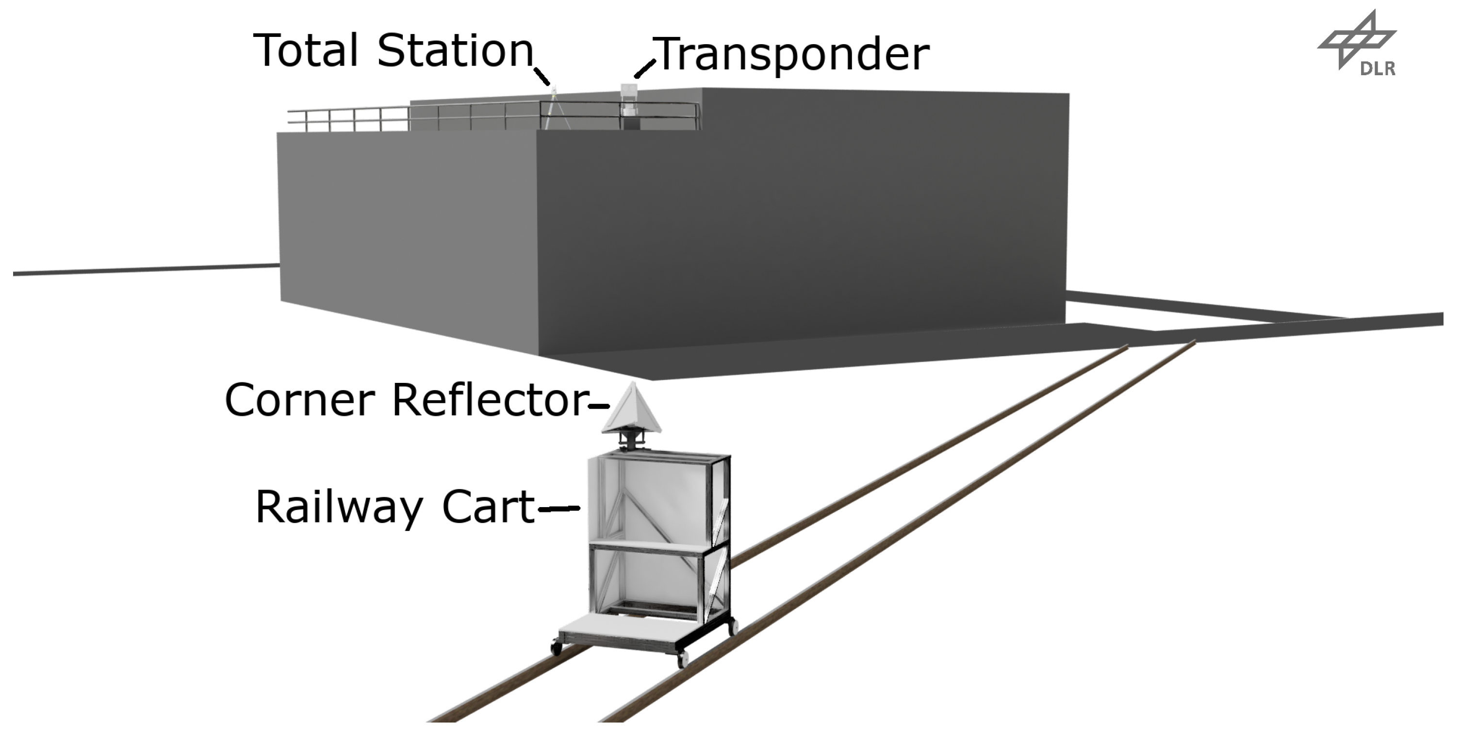
In order to mitigate multipath effects and to gather further statistics, the individual measurements of a setup are repeated for different distances using a railway cart on a track, see Figure 1. These measurements are combined as described in [10] to retrieve a result for each measurement setup.

From the three individual measurements of the calibration campaign, a system of equations can be formed, which is solved for the unknown absolute RCSs ${\varsigma }_A$, ${\varsigma }_B$, and ${\varsigma }_C$.

$$\begin{array}{ccc}\hfill {\varsigma }_A& =& a_{AB}·a_{AC}/a_{BC}·4\pi R^2\hfill \\ \hfill {\varsigma }_B& =& a_{AB}·a_{BC}/a_{AC}·4\pi R^2\hfill \\ \hfill {\varsigma }_C& =& a_{AC}·a_{BC}/a_{AB}·4\pi R^2\hfill \end{array}$$

(2)

The measurement and the RCS retrieval using Equation (2) can also be evaluated over the frequency, i.e., the system of equations can be solved for several frequency points within the device bandwidth, to evaluate the device’s transfer function. From this derived transfer function, the RCS (or likewise scattering coefficient) for any (sub-)bandwidth can be calculated.

3. Uncertainty Estimation

The error analysis and uncertainty estimation are essential steps in calibration activity. Without a known uncertainty, the quality of the measured value cannot be judged. The uncertainty estimation presented here will follow the GUM standard [12]. A tool for automatic uncertainty propagation [13] is used to ease the derivation of the uncertainty while processing the data. If not stated otherwise, all values are stated as standard uncertainties with a coverage factor of 1, i.e., $1\sigma$ values.

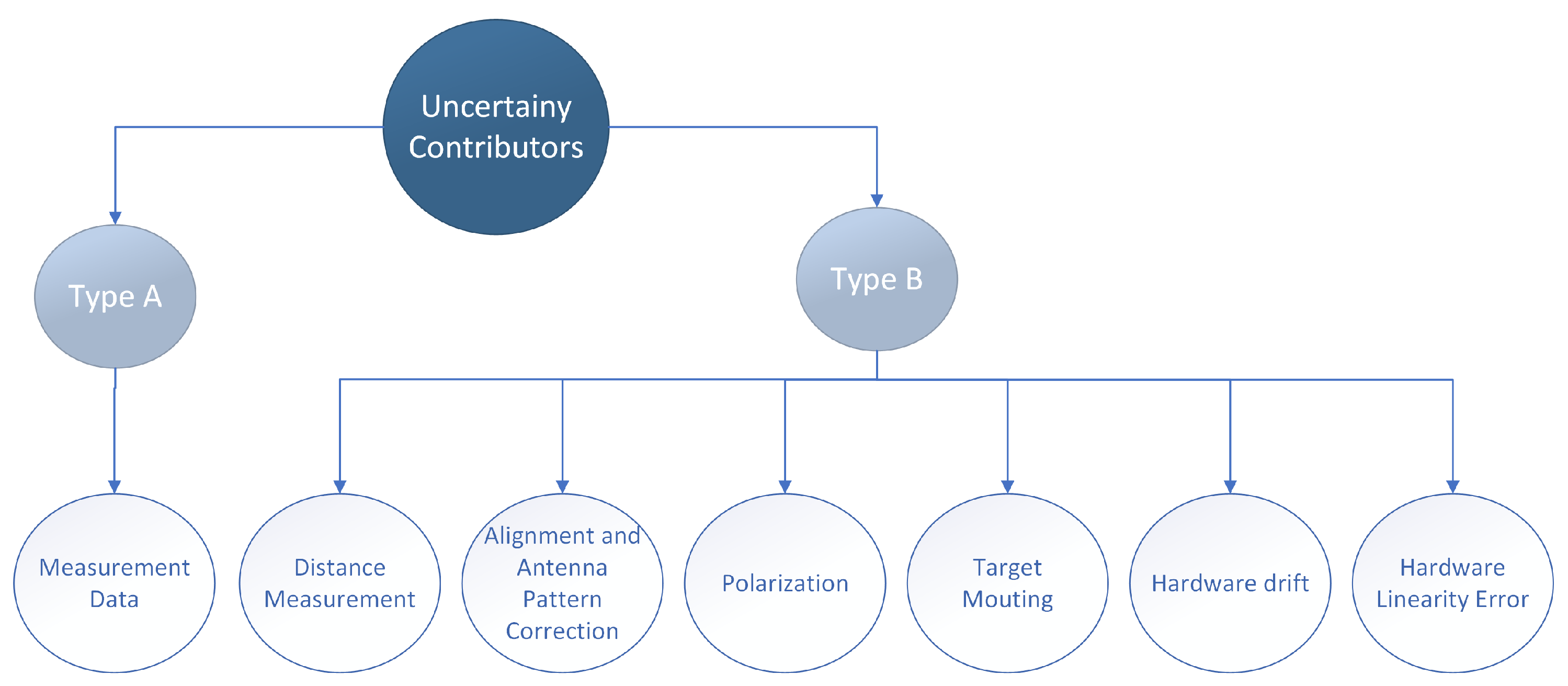
The presented uncertainty estimation will be based on GUM type A evaluations, i.e., considering the variation of the data under similar measurement conditions. The data redundancy is achieved by repeated measurements for various distances between the radar and target (i.e., different cart positions). The distance variation allows for the separation of direct and multi-path (e.g., ground reflected) signal components by their different path lengths. After compensating for all deterministic effects, the measure data should differ only by their multi-path signals and noise contributions. The type A uncertainties estimated from these data will be supplemented by type B evaluations for systematic effects, which may commonly affect all of the data. All type A and type B uncertainties will be further detailed in the following sub-sections (Section 3.1, Section 3.2, Section 3.3, Section 3.4, Section 3.5, Section 3.6 and Section 3.7) before combining them with the overall uncertainty in Section 3.8 (see Figure 2).

For the sake of simplicity, we will concentrate the analysis on the uncertainty of the magnitude of the measured data. As the RCS and gain are often reported in decibels, the uncertainty will also be expressed on a logarithmic scale. For this, the system in Equation (2) will be converted to a logarithmic scale.

$$\begin{array}{c}\hfill \left(\begin{array}{c}10·log\left({\varsigma }_A\right)\\ 10·log\left({\varsigma }_B\right)\\ 10·log\left({\varsigma }_C\right)\end{array}\right)=\frac{1}{2}\left(\begin{array}{ccc}1& 1& -1\\ 1& -1& 1\\ -1& 1& 1\end{array}\right)\left(\begin{array}{c}20·log\left(a_{AB}\right)+20·log\left(4\pi R^2\right)\\ 20·log\left(a_{AC}\right)+20·log\left(4\pi R^2\right)\\ 20·log\left(a_{BC}\right)+20·log\left(4\pi R^2\right)\end{array}\right)\end{array}$$

(3)

The combined standard uncertainty $u_c$ of the resulting value is estimated from the uncertainty $u\left(x_i\right)$ of the input quantity $x_i$ and its sensitivity coefficient $c_i$, see GUM [12]:

$$u_c^2\left(\varsigma \right)=\sum _{i=1}^N{\left(\frac{\partial \varsigma }{\partial x_i}\right)}^2{u}^2\left(x_i\right)=\sum _{i=1}^N{\left(c_{i}u\left(x_i\right)\right)}^2$$

(4)

This assumes that all uncertainties $u\left(x_i\right)$ are uncorrelated.

3.1. Uncertainty Estimation from Repeated Measurements (Type A)

The GUM type A uncertainty can be estimated from repeated measurements. After correcting for all known variations (e.g., the distance change in the data), all measurement data recorded along the cart drive range should contain redundant information. They are combined in the frequency domain as described in the first part of the paper [10]. The power ratio between the coherent frequency component (i.e., the one representing the zero frequency) and the incoherent components (all other frequency components) can be used to estimate the uncorrected variation in the measurement data and, hence, the type A uncertainty.

3.2. Uncertainty Due to Errors in the Distance Estimation (Type B)

The distance between the radar device and the target was measured using a total station, which is not error-free. The specified individual measurement uncertainties, as stated by their device specifications, are reported in

Table 1. Device uncertainties for distance measurement [14].

Device	Uncertainty ($1\mathit{\sigma }$)
Total station distance measurement on prism	1 mm + $1.5$ ppm
Total station distance measurement on surface	2 mm + 2 ppm
Total station angle measurement	1″ ($\approx 0.3\mathrm{mgon}\approx 0.27\times {10}^{-3}deg$)
Prism GRZ122 (used for tracking the cart)	2 mm (3D)
Prism GMP111 (used for the alignment of targets)	2 mm (3D)

. The measurement of the corner reflector apex was performed directly on the metal surface without a prism. For all other distance measurements, the values reported for the prisms are valid.

The uncertainty of the antenna phase center position within the antenna is assumed to be 5 mm orthogonal to the radiation direction and 20 mm along the radiation direction. This also includes the potential variation of the phase center over the frequency.

The sensitivity of the RCS estimation with respect to distance errors can be calculated from Equation (3) using Equation (4), and results in:

$$\left|c_R\right|=\left|\frac{\partial \varsigma }{\partial R}\right|=\left|\frac{40}{ln\left(10\right)·R}\right|\approx 17.37·R^{-1}$$

(5)

Hence, the sensitivity $c_R$ is highest for the smallest distance R of about 60 m with $c_R\approx 0.290 {\mathrm{m}}^{-1}$.

The final distance measurement uncertainties are listed for each measurement setup in

Table 2. Contributors to the uncertainty of distance measurements for all individual measurement setups. The uncertainties of the measurements are automatically evaluated [13] based on the uncertainties for the total station and the prisms. The total range uncertainty in dB is derived using Equation (5).

VNA—Transponder
Setup geometry	elevation	(7.2736 ± 0.0059) deg to (8.4510 ± 0.0068) deg
	azimuth	(−109.1653 ± 0.0064) deg to (−105.8935 ± 0.0074) deg
	radial distance	(61.973 ± 0.029) m to (70.921 ± 0.029) m
VNA orientation	elevation	(7.63 ± 0.53) deg
	azimuth	(−107.42 ± 0.26) deg
	Line-of-sight rotation	(0.05 ± 0.38) deg
Transponder orientation	elevation	(−8.37 ± 0.14) deg
	azimuth	(71.58 ± 0.15) deg
	Line-of-sight rotation	(0.13 ± 0.23) deg
Total range uncertainty		$28.64$ mm
		$0.00803$ dB
Transponder—Corner Reflector
Setup geometry	elevation	(−8.5453 ± 0.0086) deg to (−7.3699 ± 0.0075) deg
	azimuth	(70.3132 ± 0.0071) deg to (73.4514 ± 0.0081) deg
	radial distance	(63.236 ± 0.020) m to (72.253 ± 0.020) m
Transponder orientation	elevation	(−8.29 ± 0.26) deg
	azimuth	(72.04 ± 0.16) deg
	Line-of-sight rotation	(−0.11 ± 0.41) deg
Corner reflector orientation	elevation	(7.917 ± 0.064) deg
	azimuth	(−113.891 ± 0.065) deg
	Line-of-sight rotation	(−0.152 ± 0.026) deg
Total range uncertainty		$20.471$ mm
		$0.00566$ dB
VNA—Corner Reflector
Setup geometry	elevation	(−9.1295 ± 0.0078) deg to (−7.8844 ± 0.0068) deg
	azimuth	(70.3303 ± 0.0061) deg to (73.4707 ± 0.0069) deg
	radial distance	(63.143 ± 0.020) m to (72.113 ± 0.020) m
VNA orientation	elevation	(−8.44 ± 0.23) deg
	azimuth	(71.994 ± 0.099) deg
	Line-of-sight rotation	(−0.09 ± 0.10) deg
Corner reflector orientation	elevation	(7.917 ± 0.064) deg
	azimuth	(−113.891 ± 0.065) deg
	Line-of-sight rotation	(−0.152 ± 0.026) deg
Total range uncertainty		$20.279$ mm
		$0.00563$ dB

together with the resulting uncertainty for the RCS estimation.

3.3. Alignment and Antenna Pattern Correction (Type B)

From the geometric measurement data, which are summarized in Table 2, it can be seen that the targets were well aligned to the setup geometry, i.e., the radar device and the target were well aligned to each other. Only the corner reflector was intentionally misaligned by 3${}^{\circ }$ to 6${}^{\circ }$ to avoid the direct boresight direction of the corner reflector. Reflections of the radar-induced surface currents on the corner edges caused an RCS oscillation over frequency, which is most prominent at the boresight. Simulations with FEKO confirm the theoretical behavior. Thus, to circumvent the frequency-dependent corner reflector RCS, the boresight direction was avoided and a slightly lower off-boresight RCS was accepted instead.

Due to the cart movement, the alignment was slightly changing throughout a measurement run. The total angular change was approximately 1° in elevation and 3° in azimuth. This causes variation in the radiation pattern, which needs to be compensated for.

The radiation pattern of the trihedral corner reflector in azimuth $\theta$ and elevation $\psi$ (counted from the horizontal base plate) can be approximated by [15]:

$${\varsigma }_{trihedral}(\psi ,\theta )=\left\{\begin{array}{cc}\frac{4\pi }{{\lambda }^2}{a}^4{\left(\frac{4c_1{c}_2}{c_1+c_2+c_3}\right)}^2\hfill & \mathrm{for}{c}_1+c_2\le c_3\hfill \\ \frac{4\pi }{{\lambda }^2}{a}^4{\left(c_1+c_2+c_3-\frac{2}{c_1+c_2+c_3}\right)}^2\hfill & \mathrm{for}{c}_1+c_2\ge c_3\hfill \end{array}\right.$$

(6)

with the inner leg length a, $c_1=sin\psi$, $c_2=cos\psi sin\theta$, and $c_3=cos\psi cos\theta$, such that $c_1\le c_2\le c_3$. In addition, a correction factor is applied, which accounts for the small bistatic angle (about $0.3$ deg) caused by the separation of the transmit and receive antenna of the radar device. This correction is determined by a FEKO MLFMM (multilevel fast multipole method) simulation and has a magnitude of about 0.11 dB to 0.16 dB (frequency dependency).

The radiation patterns used for the VNA and transponder were measured and, for the transponder, compared to simulation results. The data were fitted using a logarithmic 2D Gaussian model and applied in accordance with the angular deviation between the target and boresight.

The uncertainties of the antenna pattern correction, i.e., the remaining errors after the antenna pattern correction, are hard to estimate. Instead, the data along the railway cart movement direction is tested for normal distribution. The measurement noise can safely be assumed as Gaussian. If any significant variation or drift overlays the measurement noise, the assumed normal distribution is no longer valid. If, on the other side, the data are normal-distributed, it can be assumed that no variation is present, or the drift is not significant and, hence, can be incorporated in the measurement noise, which is implicitly estimated and included in the uncertainty budget during the type A uncertainty evaluation.

To check the data for normal distribution, the Anderson–Darling test [16] was chosen, which is known to have great test power. The test value $A^2$ has to be larger than 1.09 to reject the null hypothesis with a significant level of 1%. For the measured time domain data at the target peak, the test statistic is 7.9 for the VNA vs. transponder case, 13.19 transponder vs. corner reflector case, and 1.42 VNA vs. corner reflector case. This indicates that the data along the range are Gaussian-distributed and, hence, no significant tendency (e.g., a remaining antenna pattern) is contained in the data.

3.4. Polarization Errors (Type B)

An orientation error around the line-of-sight can result in a power loss from the transmitter (radar device) to the receiver (target device) due to a polarization mismatch of the linearly polarized antennas. A potential mismatch of the polarization between the transmit and receive antenna of the transponder of the radar device is considered a property of the device. This affects the overall device’s RCS but is not considered an ’uncertainty contribution’ to the measurement setup. An orientation error of the whole device (i.e., common for the transmit and receive antennas) is considered a correctable error and the uncertainty of the orientation has to be considered in the uncertainty budget.

The polarization loss factor (PLF) can be calculated as:

$$PLF=\left|\overrightarrow{E_1}·\overrightarrow{E_2}\right|$$

(7)

where $\overrightarrow{E_1}$ and $\overrightarrow{E_2}$ are the Jones vectors of the antenna polarization. The Jones vector itself can be calculated from the orientation angle $\varphi$ and the ellipticity $\tau$ of the polarization ellipse:

$$\overrightarrow{E}=\left(\begin{array}{c}cos\varphi cos\tau -jsin\varphi sin\tau \\ sin\varphi cos\tau +jcos\varphi sin\tau \end{array}\right)$$

(8)

It is assumed that only a polarization mismatch based on the device orientation has to be considered, as the magnitude of the cross-polar term of all antennas is better than $-30$ dB and, hence, the error (due to the ellipticity) will be neglected ($\tau =0$).

For the VNA vs. transponder combination, the orientation of both devices in the line-of-sight is determined by the global position and alignment measured by the total station. The deviation in the absolute orientation angle (around the light-of-sight alignment) is better than 1 deg, resulting in a known one-way polarization loss factor that is better than $\left|\frac{\partial PLF}{\partial \varphi }\right|·1\mathrm{deg}\approx 0.0013\mathrm{dB}$.

Likewise, the uncertainty of the orientation estimation can be translated into an uncertainty of the PLF (unknown orientation angle). This uncertainty is estimated from the uncertainty of the total station data (see Table 2, polarization alignment) and is better than $0.44$ ${}^{\circ }$, resulting in a standard uncertainty of $0.00052$ dB for the PLF.

Measurements targeting the corner reflector are not affected by errors in the polarization orientation as the orientation angle of the scattering wave is not altered by a trihedral corner reflector.

3.5. Uncertainty Due to the Mounting of the Radar Target (Type B)

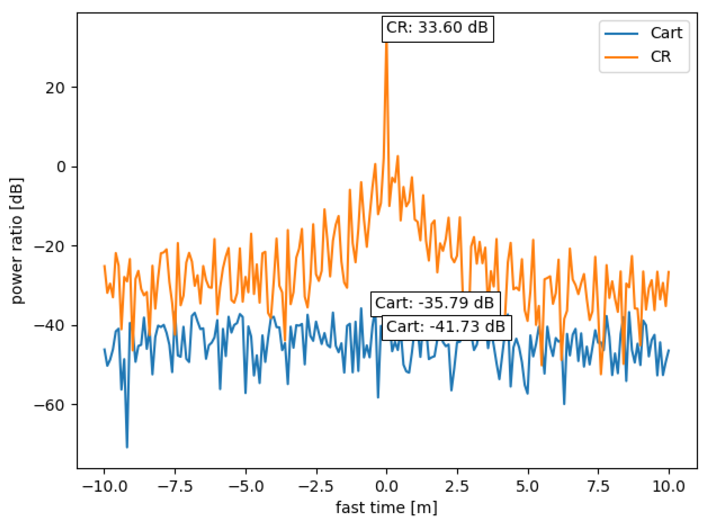
When measuring the passive radar target (i.e., the corner reflector), mechanical mounting is, in general, unavoidable, which results in additional unintended reflections. For the measurement setups, which included the corner reflector, the reflector was installed on the railway cart and the cart itself had to be treated as unwanted (mostly coherent) clutter, yielding to an uncertainty contribution. A dedicated measurement setup was carried out to characterize the RCS of the railway cart (without the mounted corner reflector). The time-domain response of the railway cart (averaged for all cart positions) is shown in Figure 3 along with the signal caused by the cart with the mounted corner reflector.

The signal-to-clutter-ratio (SCR) is defined as:

$$SCR=\frac{P_{Signal}}{P_{Clutter}}=\frac{P_{CornerReflector}}{P_{RailwayCart}}=\frac{{\left|a_{CornerReflector}\right|}^2}{{\left|a_{RailwayCart}\right|}^2}$$

(9)

and the uncertainty caused by additional clutter can be calculated by:

$${\sigma }_{Clutter}=\frac{S_{Signal}\pm a_{Clutter}}{a_{Signal}}=1\pm \frac{a_{Clutter}}{a_{Signal}},$$

(10)

where $P_{Signal}$ is the wanted signal power, $S_{Signal}$ is the wanted signal amplitude, and $P_{Clutter}$ is the undesired clutter power. $a_{Signal}$ and $a_{Clutter}$ are the respective (complex) signal amplitudes.

If the signal-to-clutter-ratio is calculated from the peak RCS (peak corner reflector RCS to clutter RCS at this position), an SCR of $75.33$ dB is achieved, causing an uncertainty ${\sigma }_{Clutter}$ of $0.0014$ dB. For the RCS values estimated using the integral method with all values down to $-40$ dB of the peak, an integrated SCR of $67.61$ dB and a ${\sigma }_{Clutter}$ of $0.0036$ dB are reached.

In the case of the VNA versus transponder setup, the transponder acts as the target with an intrinsic delay. This allows for separating the echo caused by the transponder housing, including its mounting from the delayed transponder response. Hence, this setup was not affected by additional clutter due to any mounting.

3.6. Hardware Drift Estimation (Type B)

The active hardware components are prone to gain drifts during the measurements e.g., due to ambient temperature changes. The drift of the active devices, namely the transponder and VNA, was monitored by dedicated stable measurement loops [17]. The radar devices feature internal calibration loops, which short-cut the transmit and receive antennas and allow to route the (attenuated) transmitted signal directly into the receiver path. This signal path is periodically activated to record drift samples during the measurements.

The drift uncertainty is caused by gain variations and is estimated from the mean of the device’s frequency response. Due to the multiplicative nature of the gain drifts, the relative uncertainty with respect to the mean signal power ${\mu }^2$ is used to estimate the drift:

$$u_{VNA}=u_{TR}=\frac{Std\left({\mu }_S\left(x\right)\right)}{Mean\left({\mu }_S\left(x\right)\right)}=\frac{\sqrt{\frac{1}{N_x}{\sum }_{x=1}^{N_x}{({\mu }_S\left(x\right)-\frac{1}{N_x}{\sum }_{x=1}^{N_x}{\mu }_S\left(x\right))}^2}}{\frac{1}{N_x}{\sum }_{x=1}^{N_x}{\mu }_S\left(x\right)}$$

(11)

$${\mu }_S\left(x\right)=\frac{1}{N_f}\sum _{f=1}^{N_f}\left|S_{mon}(f,x)\right|$$

(12)

where $u_{VNA}$ and $u_{TR}$ are the uncertainties for the VNA and the transponder, $S_{mon}$ is the monitoring data from the calibration loop, f is the frequency (with $N_f$ being the number of frequency points), and x is the range position of the target device (with $N_x$ being the number of range positions). $Mean$ is the mean operator and $Std$ calculates the unbiased sample standard deviation for the given data. The uncertainties for the individual setups are listed in column Drift of

Table 3. Summary of measurement uncertainties for the individual setups.

Setup	Type A	Range	Drift	Polarization	Mounting	Linearity	Total
	Uncertainty	Uncertainty		Mismatch
VNA vs. TR	$0.0421$ dB	$0.008$ dB	$0.042$ dB	$0.001$ dB	-	$0.0579$ dB	$0.083$ dB
TR vs. CR	$0.0645$ dB	$0.0057$ dB	$0.0156$ dB	-	$0.0036$ dB	$0.01$ dB	$0.067$ dB
VNA vs. CR	$0.0516$ dB	$0.0056$ dB	$0.0083$ dB	-	$0.0036$ dB	$0.0579$ dB	$0.078$ dB
Total							$0.066$ dB

.

3.7. Linearity Error (Type B)

When changing the power level injected into an active device, linearity errors may occur. This affects the VNA and the transponder.

The VNA was always operated on with constant output power; hence, no linearity error occurred on the transmitter side. The receiver uncertainty is stated as <$0.1 \mathrm{dB}$ for input signal levels from +10 dB to −80 dB over the desired frequency range of 0.7 GHz to 24 GHz (reference: [18]). Considering the low dynamic range of less than $7.5$ dB used during a measurement setup (mainly due to distance variations), the actual uncertainty due to linearity errors was probably even lower than specified. Nevertheless, it is included with the full magnitude as equally distributed over the dynamic and frequency range. Hence, it is considered as $u_{\sigma }=\frac{1}{\sqrt{3}}·u_{min,max}=0.058\mathrm{dB}$ [12].

The linearity of the transponder was determined using the internal calibration facility, i.e., above the noise floor up to the compression point (about 1500 AD counts, which was never reached during the measurements), the deviation from linearity was measured to be about $0.01$ dB ($1\sigma$).

3.8. Combined Uncertainty

In the previous sections, the estimations of all uncertainty contributors for the measurement setups were described. The overall uncertainty is determined by the single uncertainty terms in accordance with the rules defined by GUM.

Based on Equation (4), applied to Equation (3), the sensitivity of the RCS with respect to the uncertainty of individual setups can be found as follows:

$$\left|c_{TR,CR}\right|=\left|c_{VNA,CR}\right|=\left|c_{VNA,TR}\right|=\left|\frac{\partial \varsigma }{\partial a_{AB}}\right|=\left|\frac{\partial \varsigma }{\partial a_{AC}}\right|=\left|\frac{\partial \varsigma }{\partial a_{BC}}\right|=\left|\frac{1}{2}\right|$$

(13)

The combined uncertainty is equal for all target RCSs and can be derived from Equation (4) with the known sensitivity coefficients $c_i$ as ${\sum }_{i=1}^N{\left(c_{i}u\left(x_i\right)\right)}^2$. The final results are stated in Table 3.

4. Discussion and Comparison with Other Methods

The measurement results were reported in the first part of our paper [10]. In addition, the results will be compared to estimates derived by other independent measurements and, therefore, verified in the following sections.

4.1. Corner Reflector References

The RCSs of triangular trihedral corner reflectors can be analytically calculated for a given wavelength $\lambda$ and an inner leg length l, assuming physical optics:

$${\varsigma }_{TCR}=\frac{4\pi }{{\lambda }^2}·l^4$$

(14)

A formula incorporating the corner reflector RCS’s angular dependency is given in Equation (6).

More accurately, the radar cross-section can also be estimated from simulations conducted with commercially available software tools. FEKO was used to perform a full-wave MLFMM simulation of the corner reflector using a scanned mesh (measured for the corner reflector used in the campaign, using an Artec Ray laser scanner) and a perfect electric conducting (PEC) material assumption.

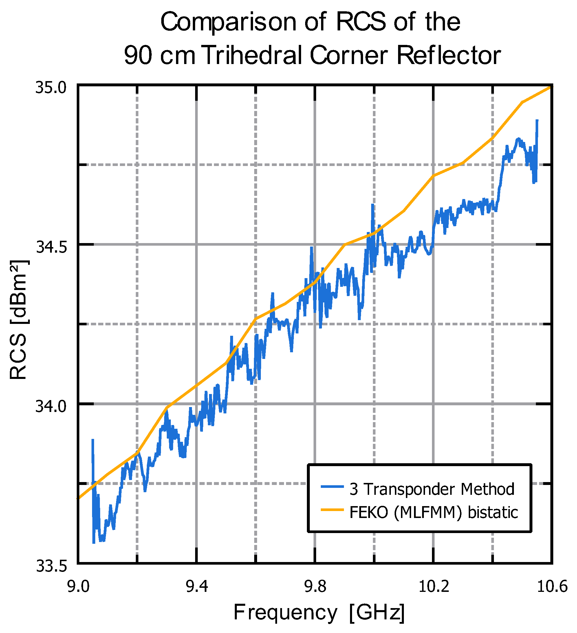
The frequency dependency of the corner reflector RCS matched well between the presented measurements and the simulation, as shown in Figure 4. The simulated angular and frequency-dependent RCS was also input into a SAR point target simulator [19] to calculate the RCS, as seen by a specific SAR sensor, such as TerraSAR-X in our case.

The different results are summarized in

Table 4. Cross-verification of the RCS estimation for the trihedral corner reflector with different methods. Note: The analytic solution is given for the center frequency while the RCSs of the other methods are stated for the defined frequency span. The FEKO simulation and the analytical solution were corrected for the small bistatic angle (see Section 3.3) by $0.13$ dB.

		FEKO Simulation,	3 Transponder Method	3 Transponder Method
	Analytical	Integrated	Measurement Result,	Measurement Result,
	Solution [dBm²]	RCS [dBm²]	Peak RCS [dBm²]	Integrated RCS [dBm²]
9.2 GHz to 10.4 GHz	34.551 @ $9.8$ GHz	34.397	34.280	34.265
9.5 GHz to 9.8 GHz	34.417 @ $9.65$ GHz	34.270	34.276	34.196

.

4.2. Transponder References

The theoretical RCS of the transponder can be estimated from the transponder’s antenna gain and its electronic gain [20]:

$$\sigma =\frac{{\lambda }^2}{4\pi }·g_{antenna}^2·g_{electronic}$$

(15)

where $g_{antenna}$ is the gain of the antennas and $g_{electronic}$ is the electric gain. The results are shown in Table 5 in the ‘Analytic result’ column.

The RCS of the transponder was also measured during an independent measurement campaign, using the TerraSAR-X mission, and compared to the measured RCS for $1.5$ m trihedral corner reflectors in the same scene. A detailed analysis can be found in [21]. This value is also reported in Table 5 in the TerraSAR-X column.

Table 5. Comparison of the peak and integrated RCS [22] retrieved by the three-transponder method, an analytical estimate according to Equation (15), and a measurement using the TerraSAR-X mission.

			3 Transponder Method	3 Transponder Method
	Analytic	TerraSAR-X	Measurement Result	Measurement Result
	Result [dBm²]	[dBm²]	Peak [dBm²]	Integrated [dBm²]
9.2 GHz to 10.4 GHz	63.72 @ $9.8$ GHz	—	62.308	62.848
9.5 GHz to 9.8 GHz	63.57 @ $9.65$ GHz	62.12	62.342	62.393

Table 5. Comparison of the peak and integrated RCS [22] retrieved by the three-transponder method, an analytical estimate according to Equation (15), and a measurement using the TerraSAR-X mission.

			3 Transponder Method	3 Transponder Method
	Analytic	TerraSAR-X	Measurement Result	Measurement Result
	Result [dBm²]	[dBm²]	Peak [dBm²]	Integrated [dBm²]
9.2 GHz to 10.4 GHz	63.72 @ $9.8$ GHz	—	62.308	62.848
9.5 GHz to 9.8 GHz	63.57 @ $9.65$ GHz	62.12	62.342	62.393

The result obtained by the analytical approach obviously has a high uncertainty as it neglects coupling and matching between the individual hardware components, losses in the antennas, and their radomes. Hence, the result is too high. The result gained from the measurements performed with the TerraSAR-X mission matched the previously presented outcome.

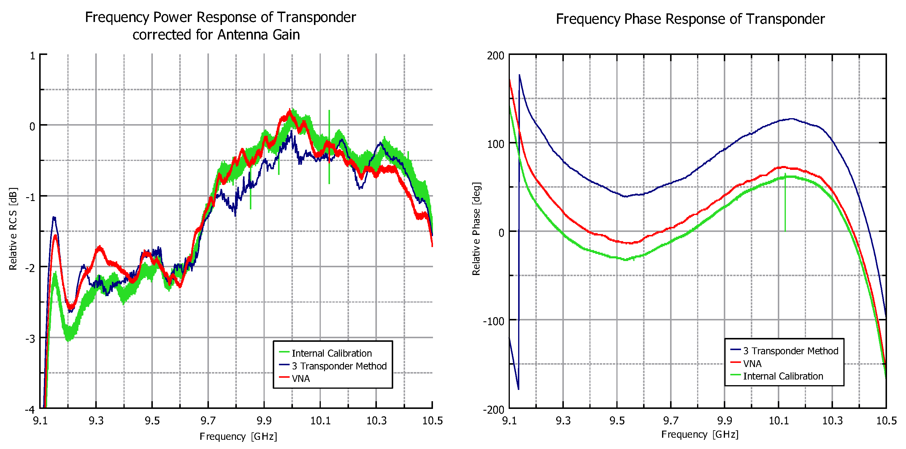
The frequency dependency of the transponder RCS can be validated against the transfer function estimated by the transponder’s internal gain compensation facility. This gain compensation facility allows routing a signal through most of the RF components by connecting the transmit RF chain with the receive RF chain via a fixed attenuator. Only the antennas and short cables are not included. Hence, the frequency response captured by the gain compensation facility is very similar to the frequency response of the whole transponder system. Additionally, the whole RF chain is characterized during the acceptance test using a VNA. The transmission is measured from the reception antenna port (with the antenna detached) to the transmission antenna port of the transponder.

All three results are depicted in Figure 5. The power of all measurements is normalized as only the three-transponder method estimates the absolute value. For a better comparison, the VNA and measurements from the gain compensation facility are corrected for the missing antenna gain in these setups. The phase response is compensated for the time delay caused by the measurement to help the interpretation of the phase without a linear phase drift due to a time delay.

The overall trend and many small features of the frequency response are similar between the various measurements. This is also true for the phase response, especially when keeping in mind that the data originate from completely different measurement setups at different times and with different ambient temperatures. Even though the differences between the measured magnitudes can be up to $0.5$ dB in some parts of the spectrum, the overall RCS can be assumed to be more accurate as determined over a given frequency range and, hence, alleviates measurement imperfections for specific frequency ranges. Thus, this comprehensive verification proves that the overall RCS is correctly determined and the frequency behavior of the transponder is correctly estimated by the novel three-transponder method.

4.3. VNA References

The radar target consists of a VNA with an attached antenna. In addition, a low-noise amplifier (LNA) and a calibration loop similar to the one in the transponder were implemented. Hence, the (virtual) RCS can be described as given in Equation (15). The RCS is stated as ’virtual’ because the VNA has no real RCS (as it cannot be operated as a target device). Nevertheless, it can be treated similar to the other devices, which have actual RCSs.

The VNA’s ’virtual’ RCS can be determined in accordance with Equation (15). The electronic gain $g_{electronic}$ is defined (assuming a well-calibrated VNA) by the attenuation in the calibration path, which is given as 60 dB. This allows for the calculation of the antenna gain $g_{antenna}$ from the (virtual) RCS. The determined gain is about $14.3$ dB while the data sheet for the used MIRAD microwave X-Band Feed System antenna states 14.5 dB at 9.5 GHz (with a resolution of $0.5$ dB).

5. Conclusions

A comprehensive measurement campaign to estimate the RCS and the complex frequency response of SAR reference targets was presented in an independently released paper [10]. In this paper, we extended the analysis by a comprehensive uncertainty evaluation along with a validation of the results. Although the measurement setup was originally designed to estimate only the RCS of a transponder, the RCS of the involved trihedral corner reflector was also estimated along the way. This allowed for an independent verification of the estimated RCS of this corner reflector with the well-established technique of full-wave finite element method (FEM) simulations. Therefore, this proves the validity of the novel three-transponder method; moreover, the theoretical RCSs obtained by the simulations correctly represent the real world, and the measurement correctly estimates the RCS. The dedicated uncertainty analysis yields a low uncertainty of only $0.066$ dB ($1\sigma$). This finally proves that the novel three-transponder method can be superior to other transponder calibration methods [8].

The low RCS uncertainty and the knowledge of the frequency dependency of the reference targets will enable a more precise external end-to-end calibration of future SAR systems. This, again, will provide users of SAR data with even better insight into the physical properties of the recorded scenes and will allow for a better interpretation of the data acquired by the SAR systems as well as their higher-level products.

Further work should focus on extending the three-transponder setup to other frequency bands, such as C-, S-, and L-bands, and demonstrating that similar uncertainties can be achieved at longer wavelengths.