Article

Multispectral Remote Sensing Monitoring of Soil Particle-Size Distribution in Arid and Semi-Arid Mining Areas in the Middle and Upper Reaches of the Yellow River Basin: A Case Study of Wuhai City, Inner Mongolia Autonomous Region

1
School of Geosciences & Surveying Engineering, China University of Mining & Technology (Beijing), Beijing 100083, China
2
School of Environment Science & Spatial Informatics, China University of Mining & Technology, Xuzhou 221116, China
*
Author to whom correspondence should be addressed.
Remote Sens. 2023, 15(8), 2137; https://doi.org/10.3390/rs15082137
Submission received: 3 March 2023 / Revised: 16 April 2023 / Accepted: 17 April 2023 / Published: 18 April 2023

Abstract

:
Particle size distribution is an important characteristic of reclaimed soil in arid and semi-arid mining areas in western China, which is important in the ecological environment protection and control of the Yellow River Basin. Large-scale coal resource mining disturbances have caused serious damage to the fragile ecological environment. The timely and accurate dynamic monitoring of mining area topsoil information has practical significance for ecological restoration and management evaluation. Investigating Wuhai City in the Inner Mongolia Autonomous Region of China, this study uses Landsat8 OLI multispectral images and measured soil sample particle size data to analyze soil spectral characteristics and establish a particle size content prediction model to retrieve the particle size distribution in the study area. The experimental results and analysis demonstrate that: (1) the 6SV (Second Simulation of the Satellite Signal in the Solar Spectrum Vector version) atmospheric correction model is more accurate than the FLAASH (Fast Line-of-sight Atmospheric Analysis of Hypercubes) model in arid and semi-arid areas with undulating terrain; (2) 0–40 cm is the optimum soil thickness for modeling and predicting particle size content in this study; and (3) the multi-band prediction model is more precise than the single-band prediction model. The multi-band model’s sequence of advantages and disadvantages is SVM (Support Vector Machine) > MLR (Multiple Linear Regression) > PLSR (Partial Least Squares Regression). Among them, the 6SV-SVM model has the highest precision, and the prediction precision R2 of the 3 particle sizes’ contents is above 0.95, which can effectively predict the soil particle-size distribution and provide effective data to support topsoil quality change monitoring in the mine land reclamation area.

1. Introduction

Soil texture is crucial in determining soil porosity, permeability, and water-holding capacity. It is closely related to soil aeration, fertilizer retention, water retention, and difficulty in cultivation [1]. The middle and upper reaches of the Yellow River Basin are the main producing areas of China’s coal industry, and large-scale mining disturbance has seriously impacted the fragile soil ecological environment [2,3,4]. In recent years, the Chinese government has issued and implemented a series of regulatory documents to strengthen land reclamation and soil ecological environment management in arid and semi-arid coal mining areas of the Yellow River Basin [5,6]. Simultaneously, soil texture is an important basis for formulating soil utilization, management, and improvement measures. Monitoring soil particle-size distribution changes during mining reclamation is a key indicator for evaluating the success or failure of land reclamation in mining areas [7,8]. Therefore, a long-term, effective, and rapid monitoring method for soil particle-size content and distribution information is essential for ecological restoration and topsoil reconstruction in arid and semi-arid mining areas.
Spectral characteristics, as an effective indicator for analyzing gradual topsoil change, are significantly affected by the difference in the content of varying soil particle sizes [9]. With the increasing development of remote sensing technology and the continuous improvement of sensor resolution, remote sensing technology is widely used for quantitatively monitoring soil physical and chemical properties [10,11,12,13,14]. At present, remote sensing images of bare soil and the spectral reflectance of soil samples are successfully used to accurately and quickly estimate soil properties [15,16,17,18,19,20,21]. Among them, multispectral image data have the characteristics of rich information, large spatial scale, and low cost. They can not only establish high-precision prediction models but also visualize the inversion results through images, which is conducive to exploring different soil particle sizes’ spatiotemporal distribution patterns [22].
The research shows that soil texture is significantly correlated with soil reflectance in VIS-NIR (visible light and near-infrared bands: 400–2500 nm) [23,24,25,26]. Calculating the surface reflectance in remote sensing images is mostly based on the MOTRAN4+ (Moderate Resolution Model for LOWTRAN4+) radiation transfer model, with fixed input parameter modes, low temporal and spatial resolution, and susceptibility to interference from the study area’s characteristics, thus resulting in limited calculation accuracy [27]. Using the 6SV (Second Simulation of the Satellite Signal in the Solar Spectrum Vector version) model combined with high-spatial and -temporal-resolution auxiliary meteorological data, surface reflectance data in areas with significant surface fluctuations, such as mines are efficiently calculated [22,28].
Multiple Linear Regression (MLR), Partial Least Square Regression (PLSR), Random Forest (RF), Support Vector Machine (SVM), and other statistical methods can be used to model the measured soil reflectance to predict the soil texture [29,30,31,32,33,34]. In recent years, machine learning methods have been more widely used in modeling and predicting soil texture characteristics and their spatial distribution, using multiple remote sensing images and using different data processing and modeling methods to improve the model’s predictive performance [1,35,36]. Currently, Ensemble Learning integrates multiple models through specific strategies to achieve higher accuracy using densely distributed datasets. However, since each model has its own advantages and disadvantages in its specific situation, choosing a specific model for predicting soil properties in a specific region or environment remains a huge challenge [37]. The SVM method based on the radial basis kernel function (RBF-SVM) shows that it can be effectively applied to VIS-NIR modeling to predict soil particle sizes. It does not require large data sets. Selecting the correct kernel function in a high-dimensional space can have a very strong robustness modeling effect [7,38].
Simultaneously, studies have shown that the relationship between spectral reflectance and soil texture is influenced by factors such as soil moisture and surface vegetation cover. When testing from experiments to large-scale use on site, changes in surface states may result in significant deviations in its accuracy [21,39,40,41]. The open-pit coal mining area in the middle and upper reaches of the Yellow River Basin in western China, with its specific arid climate conditions and disturbance factors, greatly reduces the impact of factors such as soil moisture and vegetation cover on the monitoring of soil texture using reflectance spectroscopy, effectively improving the model’s prediction accuracy, while also limiting the model’s applicable environmental range to a certain extent [7,42].
Effective methods for the dynamic monitoring and evaluation of surface soil information in mining areas are urgently needed to address ecological environment management and carry out ecological restoration and land reclamation work after mining destruction. This article uses Wuhai City, Inner Mongolia Autonomous Region, China, as an example, using Landsat8 OLI multispectral image data, aiming to (1) study the characteristics of arid and semi-arid soil reflectance spectra and the accuracy difference of different atmospheric correction models in calculating surface reflectance, (2) analyze the correlation between soil reflectance spectra and different particle sizes’ contents and determine the optimum soil thickness for studying and predicting particle sizes’ contents, (3) establish the prediction model of multiple particle sizes’ contents by performing statistical analysis of single-band and multi-band data, and (4) use the optimum model to calculate the inversion results of different particle sizes’ contents in the study area.

2. Data and Methods

2.1. Experimental Scheme

To realize the multispectral remote sensing monitoring of the soil particle-size distribution in arid and semi-arid mining areas, the following experimental scheme was designed (Figure 1): first, field soil sampling and sample analysis were conducted in the study area to obtain the soil particle-size data; second, the appropriate multispectral remote sensing images were selected and preprocessed to obtain atmospheric apparent reflectance data; third, data processing and analysis was performed, the surface reflectance data were calculated using the atmospheric correction model, and, then, the soil’s reflectance spectrum characteristics and the correlation between the three particle size contents (under different soil thicknesses) and surface reflectance data (calculated results of different atmospheric correction models) were statistically analyzed to obtain the optimum characteristic band, atmospheric correction method, and soil thickness; fourth, the single-band and multi-band models were established using the data obtained from the analysis, and the best model was selected using comparative analysis; and, fifth, the optimum model was used to retrieve the soil particle-size content and distribution information in the study area.

2.2. Overview of the Study Area

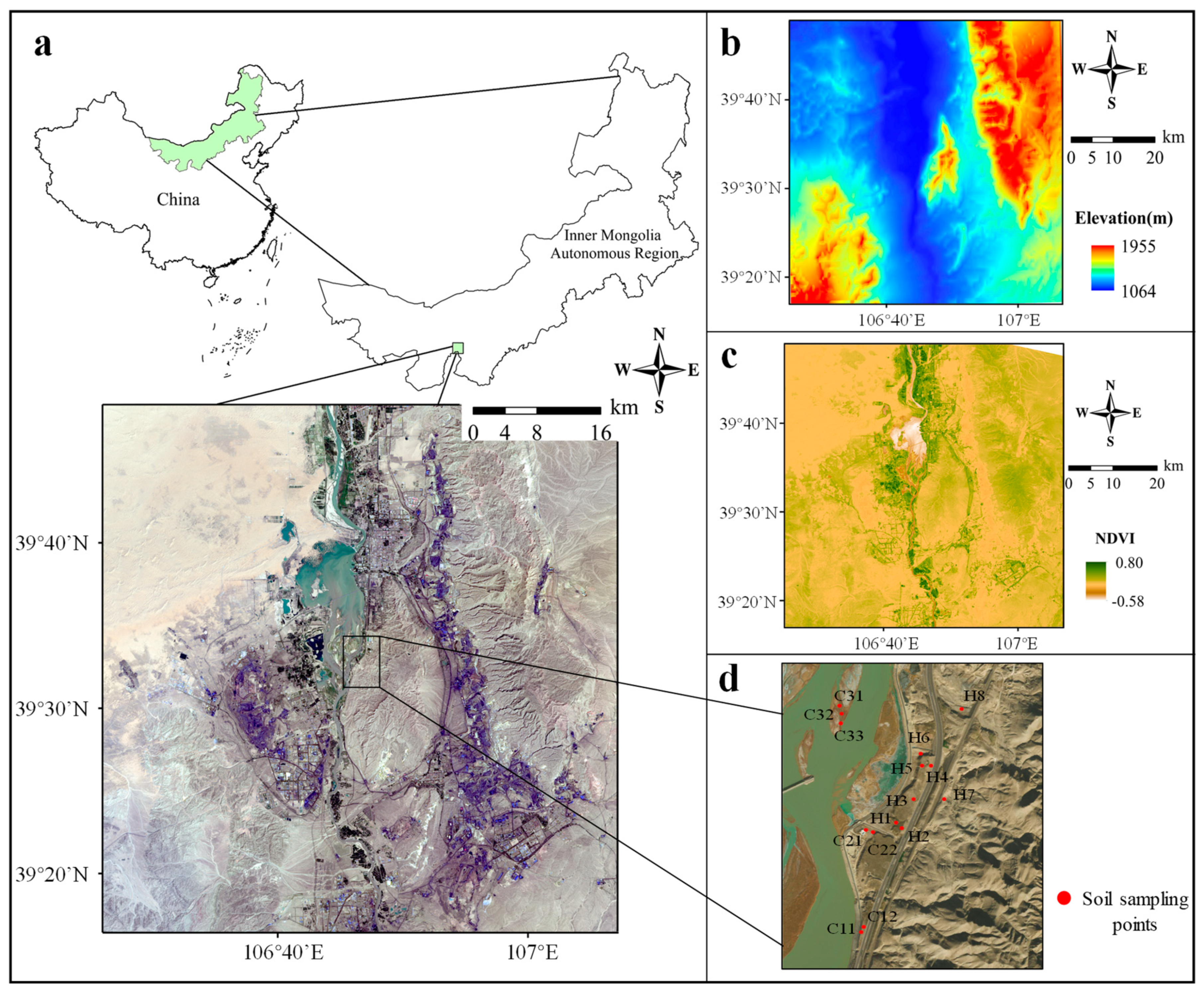
This study was carried out at the bank of Wuhai Lake in Wuhai City. The study area (39°16′3.53″–39°49′26.34″N, 106°25′41.51″–107°8′21.37″E) is in the Wuhai section of the upper reaches of the Yellow River in the Inner Mongolia Autonomous Region of China (Figure 2a). It faces the Ordos Plateau in the east, Shi Zui Shan City in Ningxia across the river in the south, A La Shan Grassland in the west, and fertile He Tao Plain in the north. Wuhai is in a typical temperate continental climate zone. Its climate is characterized by a rapid drought and temperature rise in spring, hot and high temperature in summer, concentrated precipitation and a sharp drop in temperature in autumn, and clear sky and little snow in winter. Spring and autumn are short, while winter and summer are long; the temperature difference between day and night is large, sunshine duration is long, and visible light resources are rich [43]. The annual average temperature is 282.79 K, the extreme maximum temperature is 313.35 K, the extreme minimum temperature is 236.55 K, the annual average sunshine time is 3138.6 h, the annual average solar radiation energy received is 155.8 kcal/cm2, and the average frost-free period is 156–165 days. The average precipitation over years is 159.8 mm, the average relative humidity is 42%, the average evaporation is 3289 mm, the annual average wind speed is 2.9 m/s, and the instantaneous maximum wind speed is 33 m/s. The area’s terrain is high on the east and west sides and low in the middle, with an average altitude of 1150 m [Figure 2b]. The sampling study area is the alluvial flat accumulation terrace of the Yellow River in the middle of the residual vein of the northern Helan Mountains (Zhuo Zi Mountain, Gande Er Mountain and Wuhu Mountain). The vegetation is sparse, with less than 5–10% coverage. The soil is mostly sandy loam with a loose structure, which can easily cause water and soil loss under the influence of wind and water.

2.3. Soil Sampling and Analysis

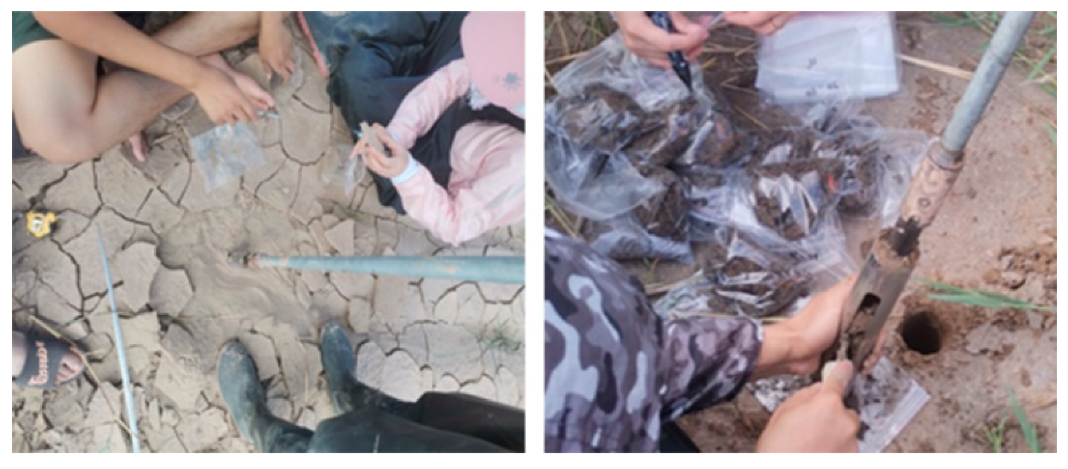
The field sampling was carried out on 22 July 2021. A total of 45 surface soil samples were collected at 15 locations near Wuhai Lake, each with 3 layers (the sampling depth is: 0–20 cm, 20–40 cm, and 40–60 cm). Soil samples were collected at each sampling point using a manual thread sampler. About 1 kg of samples was collected from each layer and separately put into sample bags, recording the sampling time, location, sample number, sampling depth, and the longitude and latitude coordinates of each sampling location using a GPS (Global Positioning System) receiver (Figure 3). The collected samples were brought back to the laboratory, the air-dried topsoil samples were screened using a standard screening technique of 2 mm, and then, the soil particle data were analyzed. According to the Chinese soil classification standard [44], each topsoil sample was divided into 6 grades: gravel (1.0–2.0 mm), coarse sand (0.25–1.0 mm), fine sand (0.05–0.25 mm), coarse silt (0.02–0.05 mm), fine silt (0.002–0.02 mm), and clay (<0.002 mm) (Figure 4). This is slightly different from the international standard: clay (<0.002 mm), silt (0.002–0.02 mm), fine sand (0.02–0.2 mm), coarse sand (0.2–2 mm), and gravel (>2 mm).
We integrated the soil particle analysis data measured in the laboratory based on the 6-level soil classification criteria into 3 categories: sand particles (0.05–2.0 mm), powder particles (0.002–0.05 mm), and clay particles (<0.002 mm). As shown in Table 1, among the soil samples tested, the average sand content of the different soil thicknesses at sampling site C (closer to the Yellow River) was higher than 61%, the average powder content was lower than 37%, and the average mucilage content was lower than 2%; the average sand content of the different soil thicknesses at sampling site H (further away from the Yellow River than C) was lower than 32%, and the average powder content was higher than 60%. The average clay content ranges from 7 to 10%. Compared with sampling site H, sampling site C has about twice as much sand, nearly half as much powder, and nearly 6% less mucilage, thus indicating that its sand content is higher, and its powder and mucilage content is lower.

2.4. Remote Sensing Image Data Selection, Processing and Analysis

2.4.1. Image Selection and Preprocessing

To use remote sensing data as auxiliary variables to predict the soil texture in the study area, we selected Landsat8 OLI images (acquired on 31 July 2021, row: 129, column: 33) that are close to the time of the field sampling. The image data were downloaded for free from the USGS (United States Geological Survey) website [45]. We used ENVI5.3 for image preprocessing, including image clipping and radiometric correction, to convert the image from the DN (Digital Number) value to the atmospheric apparent reflectance image. The calculation process involves atmospheric correction, and the specific formula is as follows:
ρ t o a = D N · g a i n + o f f s e t
In Equation (1), ρ t o a represents the atmospheric surface reflectance, D N is the remote sensing image pixels’ brightness values, which record the ground objects’ grayscale values and are directly stored in remote sensing image files, g a i n is the gain value, and o f f s e t is the offset value [46].
The NDVI (Normalized Difference Vegetation Index) is a vegetation index commonly used in remote sensing analysis [47]. The calculation formula is as follows:
N D V I = N I R R e d / N I R + R e d
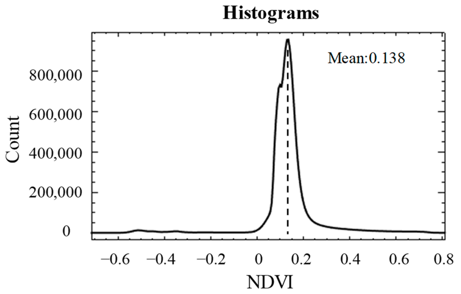
In Formula (2), N I R represents the near-infrared reflectance, and R e d represents the red reflectance. The range of N D V I is (−1, 1). The closer the value is to 1, the more likely it is to be covered with vegetation, and the closer it is to 0, the more likely it is to be bare land. After calculation, most of its values are less than 0.2 in the study area, with a mean of 0.138 (Figure 5). This shows that the surface is mostly bare when acquiring satellite data, thus meeting the experimental analysis requirements in Figure 2c.

2.4.2. Calculation of Surface Reflectivity

For the quantitative remote sensing analysis, to eliminate the influence of the cloud layer, light, and atmospheric components on the ground reflections, the atmospheric radiometric correction model was used to convert the calculation of the apparent reflectance image into the real surface reflectance data. As an auxiliary variable for the quantitative remote sensing analysis and prediction of the soil particle size, surface reflectance calculation accuracy is particularly important.
The FLAASH (Fast Line-of-sight Atmospheric Analysis of Hypercubes) model in ENVI5.3 is based on the MODTRAN4+ kernel model for atmospheric correction of the calibrated image [27]. It assumes that the surface within the solar spectral range (excluding thermal radiation) is a standard plane Lambert body, and the radiation brightness formula of a single pixel obtained by the sensor is as follows:
L * = A ρ / 1 ρ e S + B ρ e / ( 1 ρ e S ) + L α *
In Formula (3), L * is the total radiation received by the sensor; A and B are the adjustment coefficients; ρ is the surface reflectivity; ρ e is the average surface reflectivity of the pixel and the surrounding environment; S is the atmospheric spherical reflectivity; and L α * is the atmospheric backscattered radiance (atmospheric path radiation). Among these parameters, A , B , S , and L α * are calculated using the MODTRAN4+ model according to the atmospheric state and geometric conditions. After performing the atmospheric inversion, the spatial average radiation image L e * can be calculated by using Equation (3), from which Formula (4) is derived, approximately, and is used to calculate ρ e .
L e * = A + B ρ e / 1 ρ e S + L α *
As shown in Equation (3), A , B , S , L e * , and other variables also depend on the atmospheric state and geometric conditions, which are calculated using the MODTRAN4+ model and solving ρ e by introducing Equation (4). The result is interpolated into Formula (3) to solve the surface reflectivity ρ .
The 6S model was improved by Eric Vemote of the University of Maryland, United States. The 6S model considers the problems of new gas-absorbing molecules, heterogeneous ground, and bidirectional reflectivity. The calculation accuracies of the Rayleigh scattering and aerosol scattering effects were improved using the successive scattering algorithm [48]. The 6SV model is a vector version of the 6S model. Based on accurately simulating the satellite and plane observation heights, and reasonably considering factors such as anisotropy, heterogeneous surface, and non-Lambert body, it can simulate continuous and orderly scattering, calculate radiation polarization, and then solve the radiation transfer equation, which can more effectively eliminate the effects of Rayleigh scattering and aerosols [22,49].
The RSD (Remote Sensing Desktop) software is used to introduce the USGS atmospheric correction program (LaSRC) designed for Landsat8 based on the 6SV2.1 model [50]. The daily auxiliary meteorological data are calculated using USGS for LaSRC using an MODIS (Moderate-resolution Imaging Spectroradiometer). The atmospheric pressure, water vapor, ozone, and other parameters have higher temporal and spatial resolutions. The atmospheric reflectivity obtained using the 6SV model sensor is as follows:
R * θ S , θ V , Φ V = T g θ S , θ V R a θ S , θ V , Φ V + T θ S 1 R P S R C e τ μ V + R P T d θ V
In Formula (5), R * θ S , θ V , Φ V is the apparent reflectance of the top atmospheric layer accepted by the sensor, T g designates the gaseous transmission by the water vapor, ozone, or other gases, R a θ S , θ V , Φ V is the path radiation caused by the Rayleigh scattering and aerosol scattering, θ S is the zenith angle of the sun, θ V is the observation zenith angle, Φ V is the azimuth angle, T θ S is the total downlink radiation transmittance, T d θ V is the total uplink radiation transmittance, e τ μ V is the uplink radiation directly projected to the sensor, μ V = c o s θ V is the cosine of the zenith angle of the satellite, τ is the atmospheric optical thickness, R P is the non-uniform target reflectivity, and R C represents the proximity effect [49].
In this paper, two models, FLAASH and 6SV, are used for experiments to compare their calculated surface reflectance results in this study area. ENVI5.3 was used to perform the FLAASH atmospheric radiation correction on the preprocessed image, and the 6SV atmospheric correction module in the RSD software was used to invoke the auxiliary meteorological data of the imaging day to perform atmospheric correction on the image [22].

2.4.3. Statistical Analysis

The Landsat8 OLI image includes 9 wavebands, and its wavelength range is shown in Table 2. Bands 1–7 are included in the surface reflectance data calculated in this study, and the surface reflectance data of seven bands are closely related to the topsoil’s particle size distribution. The Pearson Correlation Coefficient is used to measure the correlation between the 2 variables, with a value between −1 and 1. The calculation formula is as follows:
r = i = 1 n X i X ¯ Y i Y ¯ / i = 1 n X i X ¯ 2 i = 1 n Y i Y ¯ 2
In the formula, X i represents the soil particle size content of a certain sampling point, Y i represents the surface reflectance data of a certain sampling point, n represents the number of sampling points, X ¯ is the average soil particle size content of all sampling points, and Y ¯ is the average surface reflectance of all sampling points. r represents the Pearson Correlation Coefficient, with a value less than 0 indicating a negative correlation between the surface reflectance and soil particle size content. Conversely, a value greater than 0 indicates a positive correlation between the 2. When r is closer to ± 1 , it indicates a stronger linear correlation between the 2 variables. By performing a statistical analysis for the correlation coefficient, the most appropriate atmospheric correction method, the best characteristic waveband, and the best soil thickness were selected by comparison, and then multiple prediction models of the soil particle-size distribution were established.

2.5. Modeling Process

To meet the study requirements, we plan to use the soil sample spectral data to establish a variety of prediction models for calculating the distribution of the three soil particle sizes’ contents and then select the optimum model by performing a precision comparison analysis to retrieve the soil particle size contents and distribution information in the study area. Liao analyzed the correlation between the DN value of a Landsat ETM image and soil particle size content and selected a single-feature band to estimate the topsoil texture [24]. Rossel compared different data mining algorithms to simulate soil’s reflectance spectral characteristics in a VIS-NIR band and compared various methods’ prediction effects on the clay content [31].
Multiple Linear Regression (MLR) is a regression technique that is essentially an extension of ordinary least squares regression (OLSR). MLR uses multiple explanatory variables to predict the results of response variables. Its goal is to establish a linear relationship model between multiple independent variables and dependent variables [51]. In contrast, Partial Least Squares Regression (PLSR) is also a regression modeling method of multiple dependent variables to multiple independent variables [52]. It integrates the advantages of Principal Component Analysis (PCA), Canonical Correlation Analysis (CAA), and MLR. Solving the thorny problem of multiple correlations between independent variables when there are few examples is key.
The Support Vector Machine (SVM) is a widely used machine learning method. It shows excellent classification and generalization ability in dealing with small samples, nonlinearity, etc., and is widely used in regression, classification, and other fields. Some research has also been used for VIS-NIR modeling [7]. Based on statistical theory, the SVM (RBF-SVM) method based on the radial basis kernel function is adopted. Contrary to the above PLSR model’s PCA part, this method increases the dimension of the low-dimensional eigenvalue and constructs a linear decision function in high-dimensional space to achieve a regression prediction of the nonlinear problems [38].
Combined with the optimum characteristic band obtained by performing statistical analysis and the characteristics of all the seven bands’ surface reflectance data, we established single-band and multi-band models, respectively, from two aspects:
  • For the single-band model, we define the independent variable x as a single characteristic band’s surface reflectance data, while the dependent variable y j is the particle-size content of the three different soil types. The single-band optimum fitting model of the different particle sizes was established using Origin2018 software;
  • For the multi-band model, we define the independent variable x i as all the surface reflectance data of Bands 1–7, while dependent variable y j is the content of the three different soil particle size types. The regression equation between x i and y j was established using the MLR and PLSR methods as follows:
    y j = b + i = 1 7 k i · x i
In Equation (7), j = 1 ,   2 ,   3 , where y 1 represents the sand particle content in the soil; y 2 represents silt particles; and y 3 represents clay particles. MATLAB software was used to establish different regression models and calculate the coefficients k i and b of the MLR and PLSR regression equations.
The SVM model uses the libSVM toolbox in the MATLAB software and the 2 main functions of svmtrain and svmprecict, while 70% of the data is used for training and 30% for verification. Additionally, the main parameters are set as follows: SVM type as epsilon-SVR; kernel type as Radial Basis Function (RBF); gamma as 2.8 (gamma in kernel function); cost as 1 (the parameter epsilon-SVR); and epsilon as 0.05 (the epsilon in loss function of epsilon-SVR).

2.6. Modeling Evaluation

These models use statistical values such as R 2 (R-Square), MSE (Mean Squared Error), and F-value (value of the F-test statistic) to validate the model’s predictive accuracy, and these validation metrics can be calculated according to the following Equations (5)–(7):
R 2 = 1 i = 1 m y ^ i y i 2 / i = 1 m y ¯ i y i 2
M S E = 1 m i = 1 m y i y ^ i 2
F = i = 1 m y ¯ i y i 2 i = 1 m y ^ i y i 2 / i = 1 m y ¯ i y i 2
In the above equations, y i and y ^ i are the true and predicted values of the soil particle size content, respectively. y ¯ i is the mean of a set of true values of the soil particle size content, and m is the number of samples in the model. R 2 is calculated in the range of (0, 1), and the closer to 1, the better the model effect. M S E indicates the samples’ dispersion, and the closer to 0, the better the model’s quality and the higher the prediction accuracy. The F value reflects the model’s significance, and a larger value indicates the model’s stronger overall explanatory power. Then, the above indicators are compared and analyzed, and the optimal model is selected to invert the distribution information of the soil grain size using the surface reflectance data in the study area.

3. Results and Analysis

3.1. Analysis of Surface Soil Reflection Spectra at Sampling Points

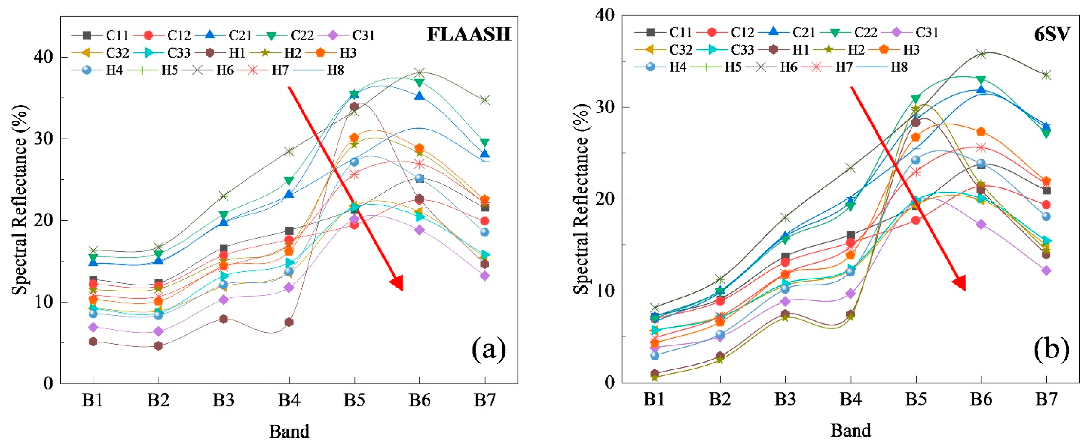
The soil surface’s reflectivity increases with the wavelength of visible and near-infrared light [9,53]. According to the United States Geological Survey’s Speclab report, soil reflectivity decreases with the increase in the grain size in the visible and near-infrared bands [54]. Figure 6 shows the topsoil sampling point’s reflection spectrum. The surface reflectance calculated by the two atmospheric correction models shows that the surface spectral reflectance is closely related to the particle-size composition of the topsoil at the sampling point. The soil surface reflectance curves calculated using the two models (Figure 6) have relatively similar spectral characteristics; except for a small amount of absorption in the red-light band, they all increase gradually in the visible near infrared band and decrease gradually in the short-wave infrared band. As shown in Figure 6, the red arrow indicates the direction of the increasing sand content and decreasing silt and clay contents of soil samples. The reflectivity decreases with the increasing sand content and increases with the decreasing silt and clay contents. In addition, due to the study area’s strong wind erosion climate conditions, there should be fewer fine particles exposed on the soil surface (as shown in Table 1, clay particles’ contents increase gradually with the increase in the soil thickness). The study area is arid and semi-arid, so the soil water-holding capacity is weak and the water distribution changes greatly. The superposition of these factors leads to the phenomenon of “wave crest moving forward” in the spectral reflection curve of the individual sampling points, but the overall trend is basically the same.

3.2. Correlation Analysis between Soil Grain Size and Surface Reflectance

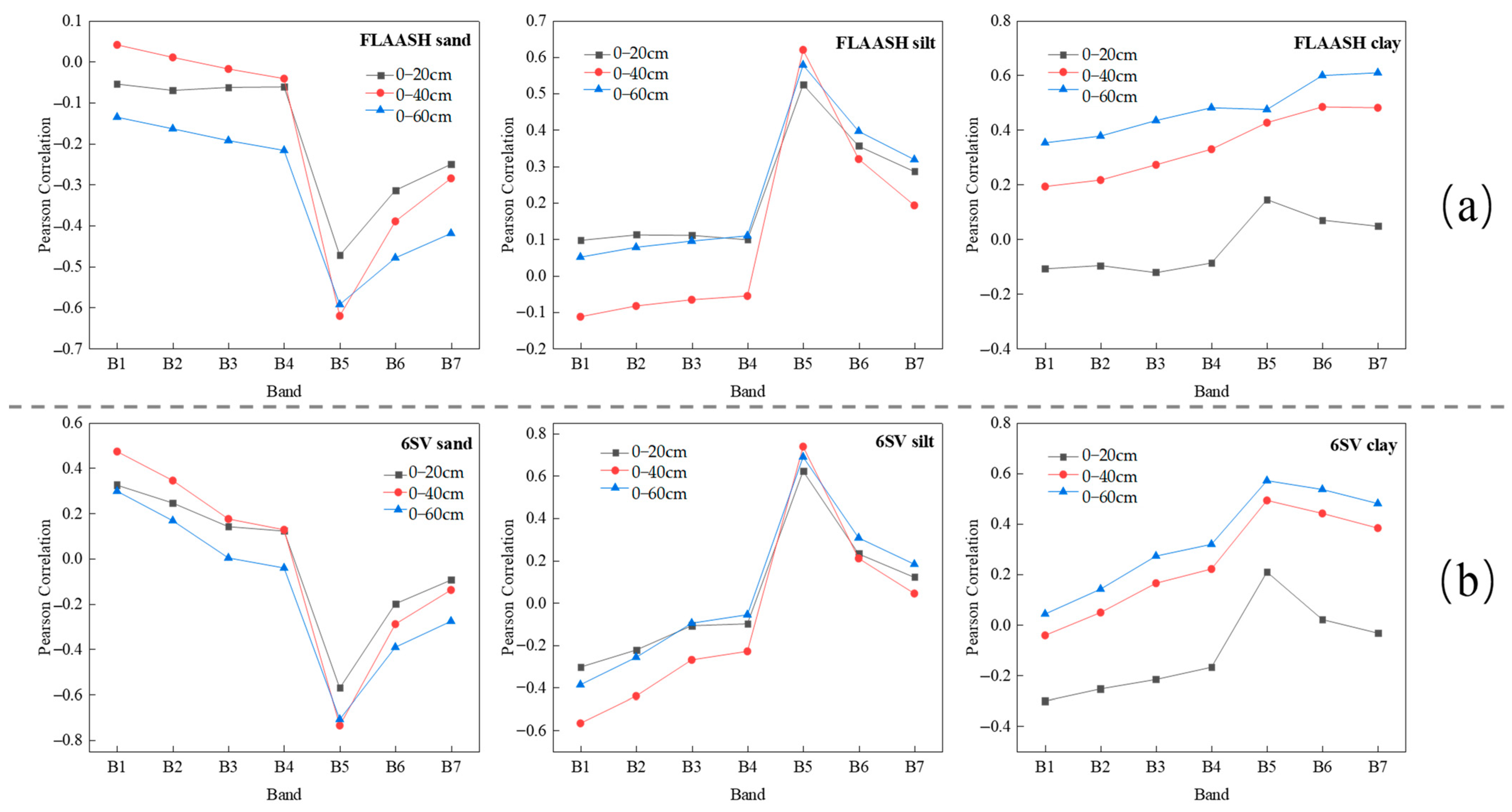
Figure 7 shows the relationship between the reflectance spectrum data calculated using the two atmospheric correction models [(a) FLAASH and (b) 6SV] and the three particle sizes’ contents (sand, silt, and clay) with different soil thicknesses (0–20 cm, 0–40 cm, and 0–60 cm). The sand content (0.05–2.0 mm) is almost all negatively correlated with the FLAASH model reflection spectrum data in B1–B7, positively correlated with the 6SV model reflection spectrum data in B1–B4, and negatively correlated with B5–B7. The correlation data of the 3 soil thicknesses showed a similar trend, in which the sand content with 0–40 cm soil thickness and most of the 2 models’ wave bands (B1–B5) showed a higher correlation than the particle size data of the other 2 soil thicknesses (0–20 cm and 0–60 cm) and showed a significant negative correlation in B5, with correlation coefficient values of −0.62 (FLAASH) and −0.73 (6SV), respectively.
The silt particles’ content (0.002–0.05 mm) is almost all positively correlated with the FLAASH model reflection spectrum data in B1–B7, negatively correlated with the 6SV model reflection spectrum data in B1–B4, and positively correlated with B5–B7. As with the sand data, the correlation data trend of the three thicknesses is similar. The silt content with 0–40 cm soil thickness and most of the 2 models’ wave bands (B1–B5) show a higher absolute correlation than the particle size data of the other 2 soil thicknesses (0–20 cm and 0–60 cm), and both show significant positive correlation in B5. The correlation coefficient values are 0.62 (FLAASH) and 0.74 (6SV), respectively.
The correlation trend of the clay content (<0.002 mm) and two kinds of reflectance spectral data are completely different from the first two. The correlation between 0–20 cm soil thickness and the reflectance spectral data of the two models is negative in B1-B4 and positive in B5–B7, and the absolute correlation is low, not exceeding 0.2 (FLAASH) and 0.3 (6SV), respectively. The correlation data of 0–40 cm soil thickness no longer have the strongest correlation, but the clay content with 0–60 cm soil thickness shows a higher absolute correlation with all the 2 models’ band data and shows the highest positive correlation in B7 and B5, respectively, with correlation coefficient values of 0.61 (FLAASH) and 0.57 (6SV), respectively.
The above analysis shows that the 0–40 cm soil thickness has the strongest correlation with the multiple wavebands’ reflectance data in both the sand and silt particle sizes. Although the clay particle data’s correlation intensity is not as strong as 0–60 cm, considering the special strong wind erosion climatic conditions in the research area mentioned above, the fine particles distributed in the soil’s upper layer may be relatively reduced to some extent, the correlation of the clay data with 0–40 cm soil thickness is reduced, and the correlation trend is similar to that of the 0–60 cm thickness soil. In addition, considering the optical remote sensing’s surface observation, the particle size content’s optimum soil thickness predicted using modeling in this study is determined to be 0–40 cm.

3.3. Model Establishment and Verification

3.3.1. Single-Band Model Analysis

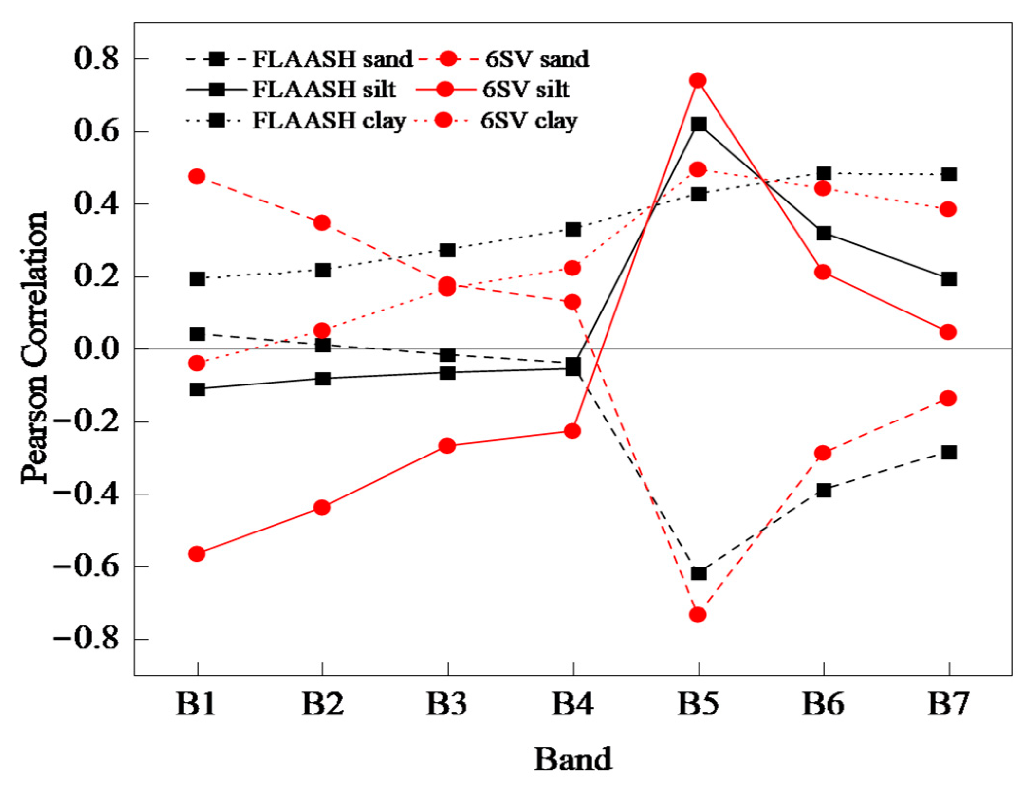
To evaluate the optimum model fitting’s performance for single-band data, the band with the highest correlation coefficient with each particle size content in the two atmospheric correction models is selected for fitting. As shown in Figure 8, the maximum Pearson correlation coefficient of the 3 particle sizes is the B5 of the 6SV model, −0.73 (sand), 0.74 (silt), and 0.50 (clay), respectively. Therefore, the land surface reflectance data of Band 5 calculated using the 6SV atmospheric correction model is finally selected for the optimum model fitting (Table 3).
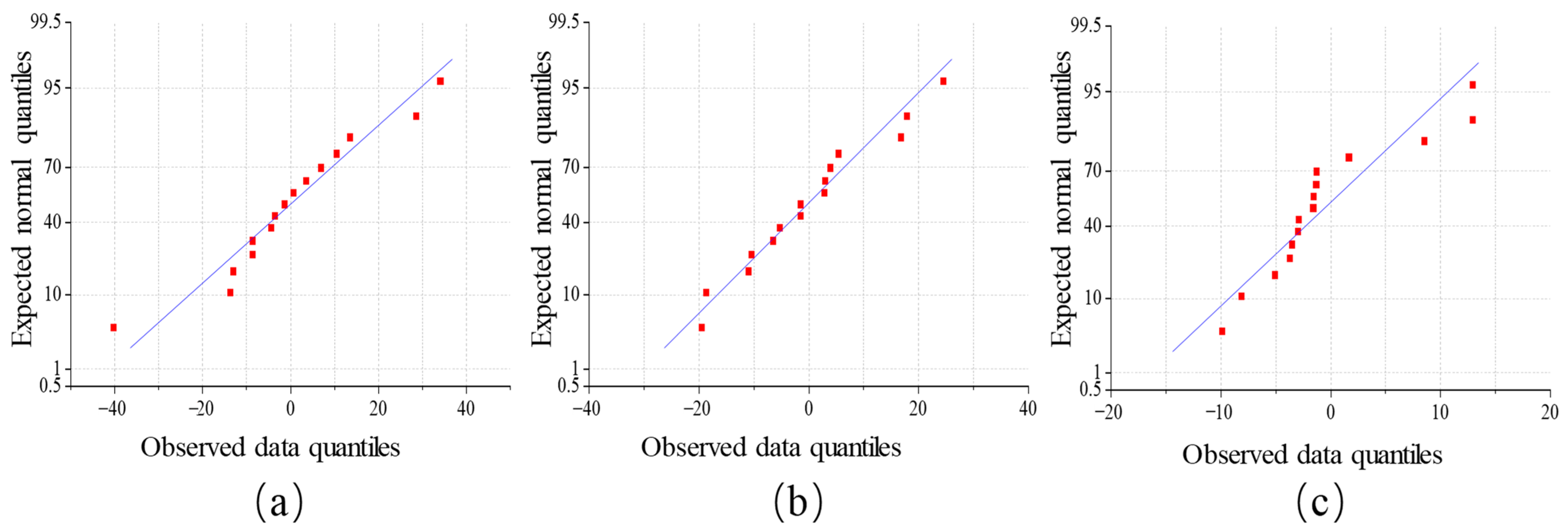
As shown in Figure 9, the Q–Q graphs of the three granularities show the conformity degree between the actual data (observed data) distribution and the theoretically calculated data distribution, testing whether the two sets of data obey the same distribution. The results show that they tend to fall in a straight line, thus indicating the experimental data’s overall normality and the established regression model’s validity. The fitting results are shown in Table 3. The sand and silt content are at the 0.05 level, and the fitting equation is obviously better than the equation y = c o n s t a n t . Among them, the silt content’s fitting model has the highest prediction ability, with adjusted R 2 = 0.518 and F = 71.415 , and the sand content’s fitting model with adjusted R 2 = 0.451 and F = 46.705 . The clay content fitting model has the worst prediction ability, with the adjusted R 2 = 0.172 and F = 17.024 , basically having no significant prediction ability.

3.3.2. Multi-Band Model Analysis

According to the multi-band surface reflectance data of FLAASH and 6SV atmospheric correction models, the MLR, PLSR, and SVM methods were used to establish prediction models for the sand, silt, and clay content in the 0–40 cm thick soil (Table 4 and Table 5). Obviously, the accuracies of the three prediction models established using 6SV correction data are better than that of the FLAASH correction data. The specific order of the model performance is 6SV-SVM > FLAASH-SVM > 6SV-MLR > FLAASH-MLR > 6SV-PLSR > FLAASH-PLSR. The data analysis shows that the precision of the particle size prediction models established using the two atmospheric correction methods are significantly different, and the 6SV model is generally superior to the FLAASH model, which is consistent with the fact that the 6SV model has a higher correlation coefficient in the correlation analysis. Thus, different atmospheric correction methods have significant differences in applicability when calculating specific areas’ surface reflectance, and their calculation results’ accuracy directly affects the soil particle-size prediction models’ accuracies.
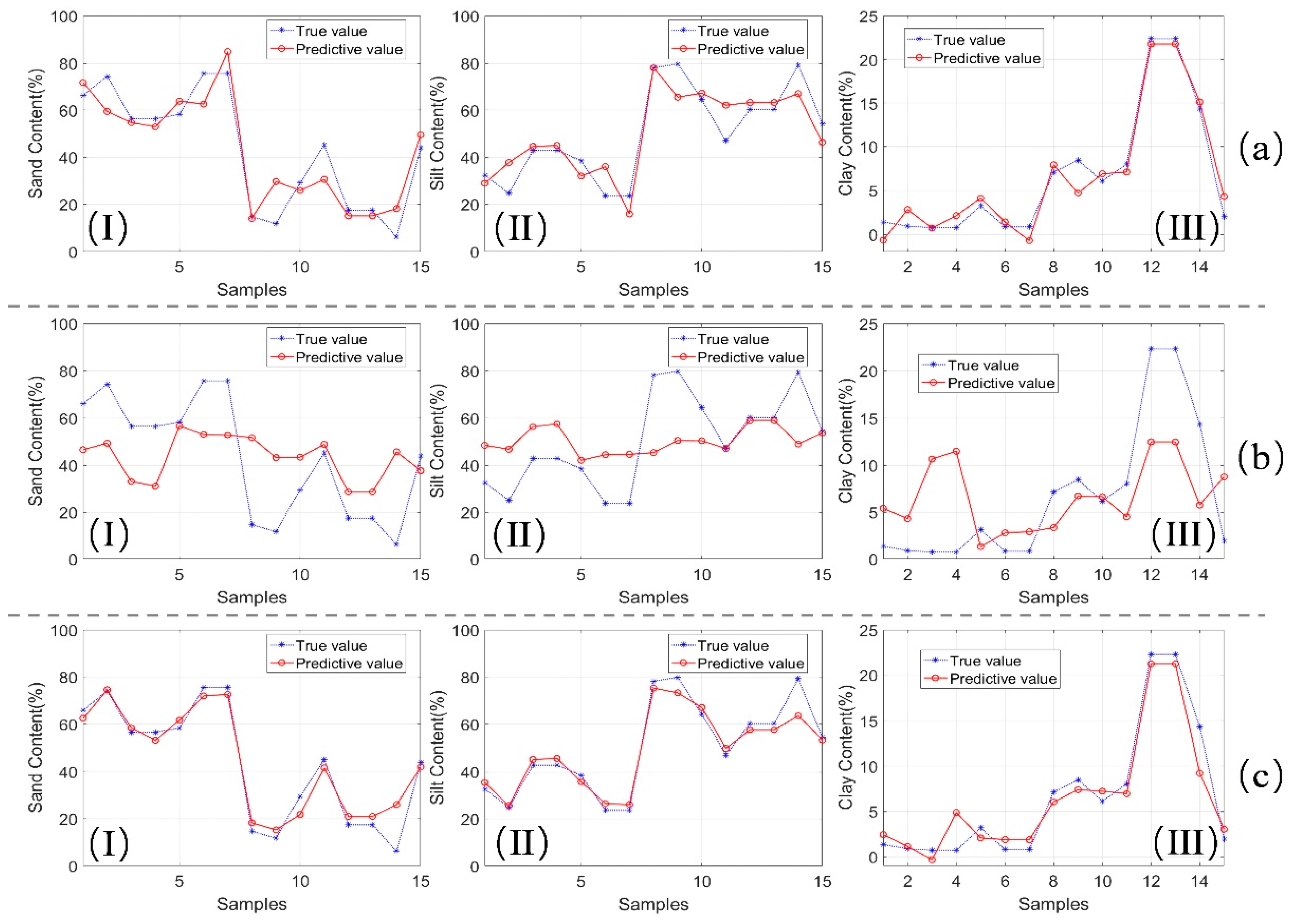
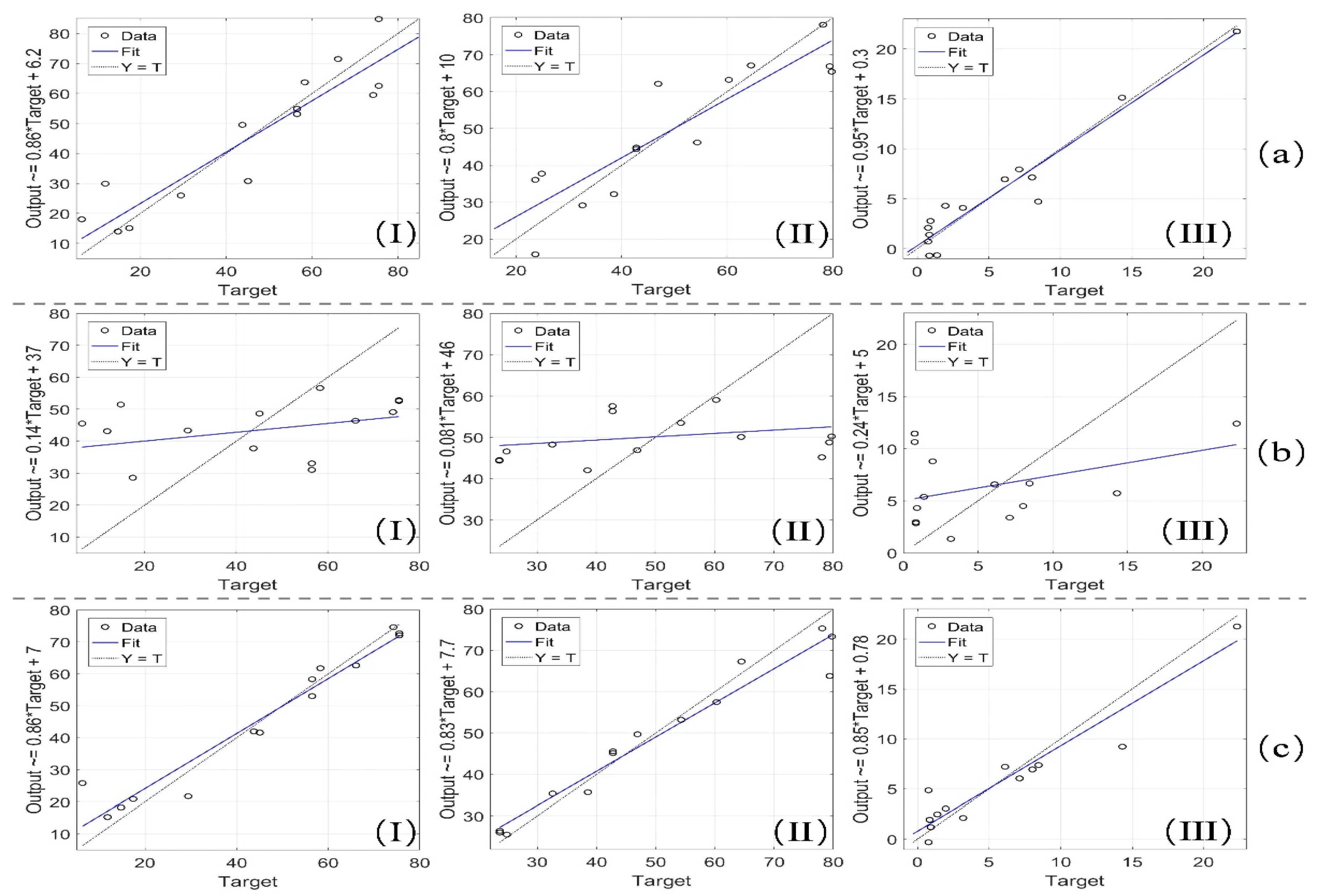
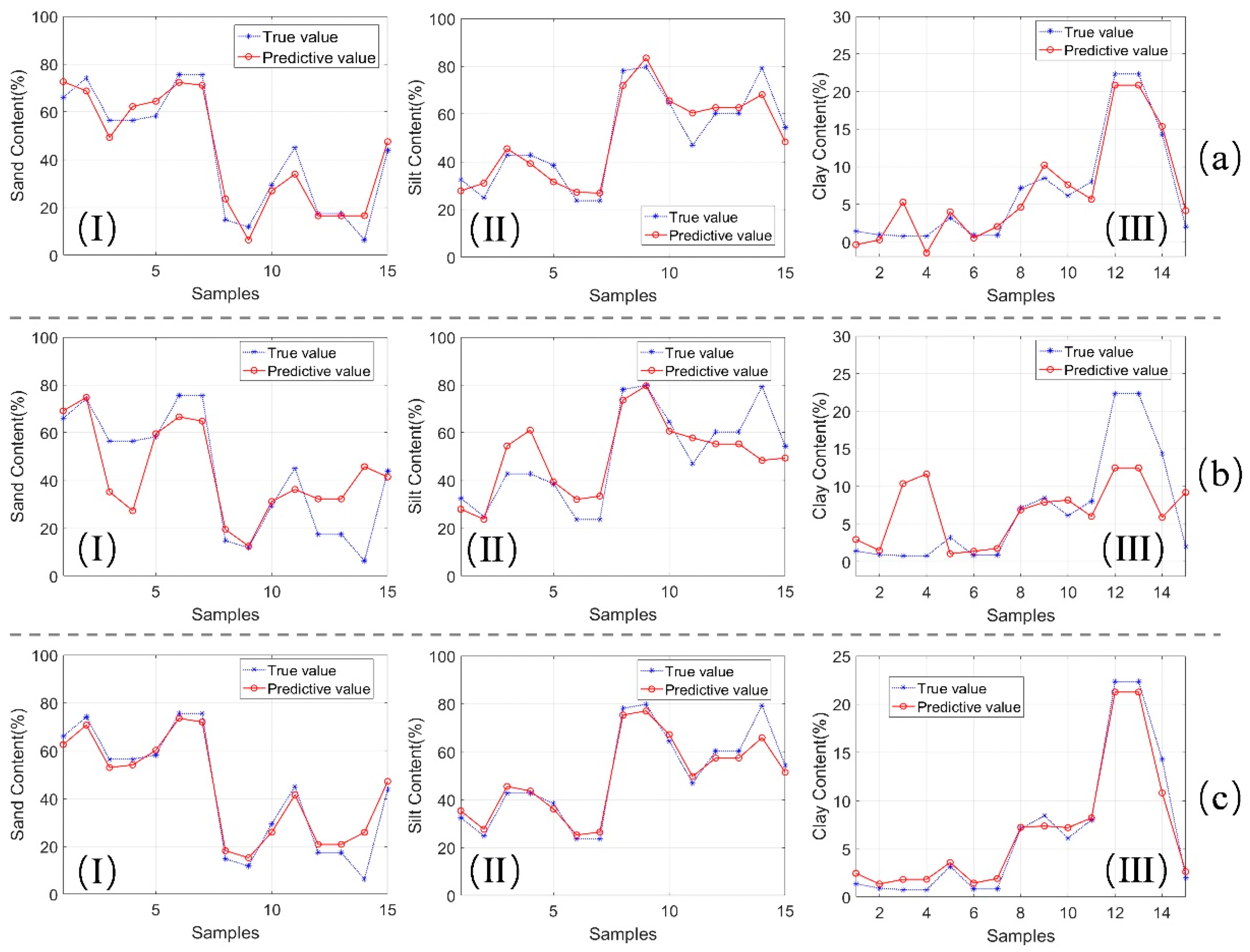
Analyzing the fitting effect diagram (Figure 10) of the predicted values and the real values of the three models established using the FLAASH correction data and the dispersion degree of points in the regression diagram (Figure 11) shows that the FLAASH-MLR model’s prediction accuracy is not very good (Figure 10a and Figure 11a). Except for the clay content, it is lower than the FLAASH-SVM model, in which R 2 = 0.856 and F = 5.948 (sand), R 2 = 0.798 and F = 3.943 (silt), and R 2 = 0.955 and F = 21.102 (clay). The particle size content prediction accuracy of the FLAASH-PLSR model is very poor (Figure 10b and Figure 11b). Among them, the clay content with the highest prediction accuracy is only R 2 = 0.240 , and the sand and clay contents are R 2 = 0.138 and R 2 = 0.081 , respectively. The generated model has no prediction ability at all. The FLAASH-SVM model has the highest prediction ability for 3 particle sizes’ contents (Figure 10c and Figure 11c), in which R 2 = 0.946 and M S E = 0.008 (sand), R 2 = 0.953 and M S E = 0.008 (silt), and R 2 = 0.936 and M S E = 0.008 (clay).
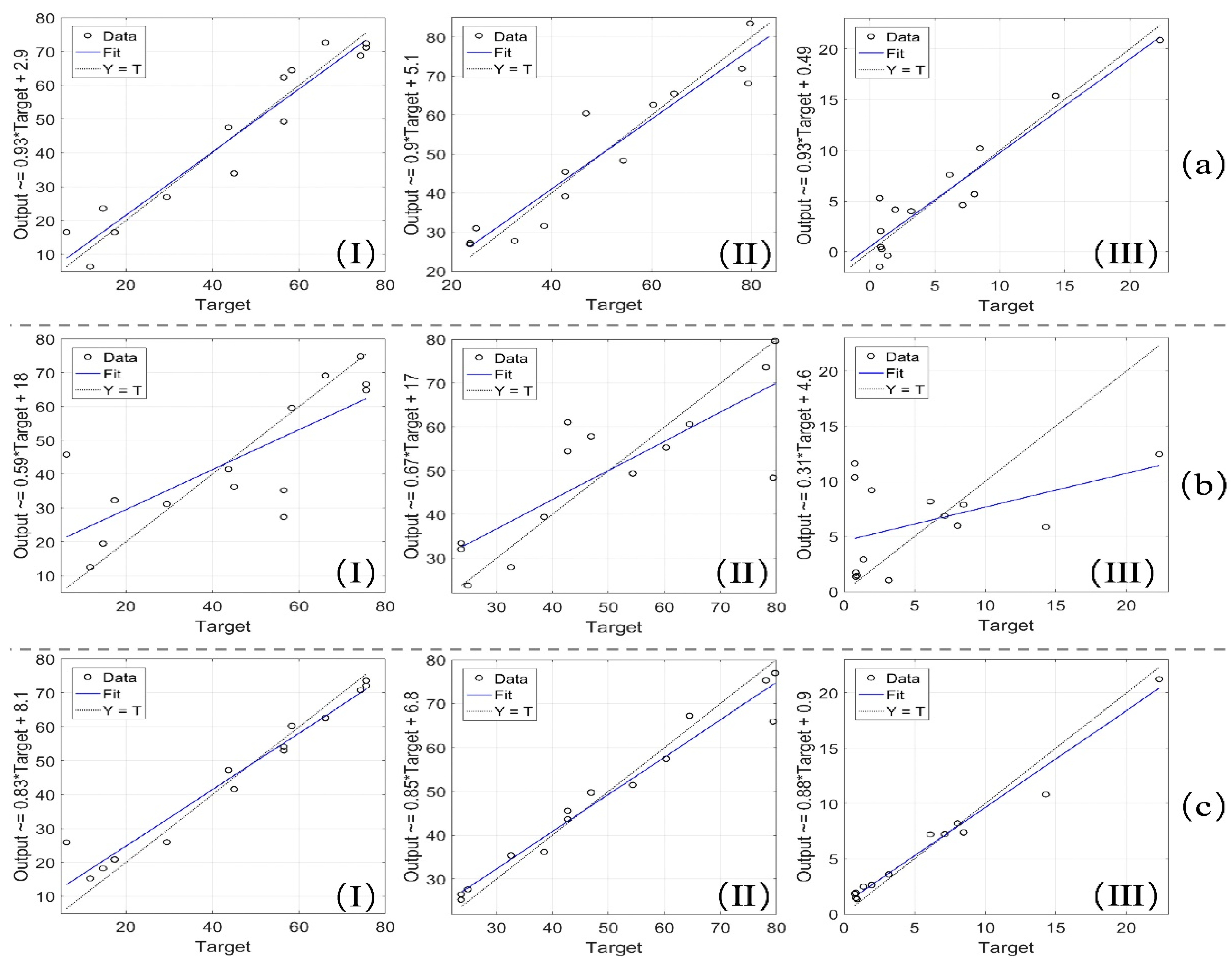
Analyzing the fitting effect diagram (Figure 12) of the predicted values and real values of the three models established using the 6SV correction data and the dispersion degree of the points in the regression diagram (Figure 13) shows that the 6SV-MLR model has good prediction accuracy (Figure 12a and Figure 13a). It is slightly lower than the 6SV-SVM model, in which R 2 = 0.934 and F = 14.129 (sand), R 2 = 0.899 and F = 8.873 (silt), and R 2 = 0.926 and F = 12.435 (clay). The particle size content prediction accuracy of the 6SV-PLSR model is the worst (Figure 12b and Figure 13b), in which the highest prediction accuracy of the silt content is only R 2 = 0.667 , while the sand and clay contents are R 2 = 0.591 and R 2 = 0.307 , respectively; and the generated model can hardly reach the prediction accuracy. The 6SV-SVM model has the highest prediction ability for 3 particle sizes’ contents (Figure 12c and Figure 13c), in which R 2 = 0.958 and M S E = 0.007 (sand), R 2 = 0.965 and M S E = 0.006 (silt), and R 2 = 0.983 and M S E = 0.003 (clay).

3.4. Inversion Results of Prediction Model

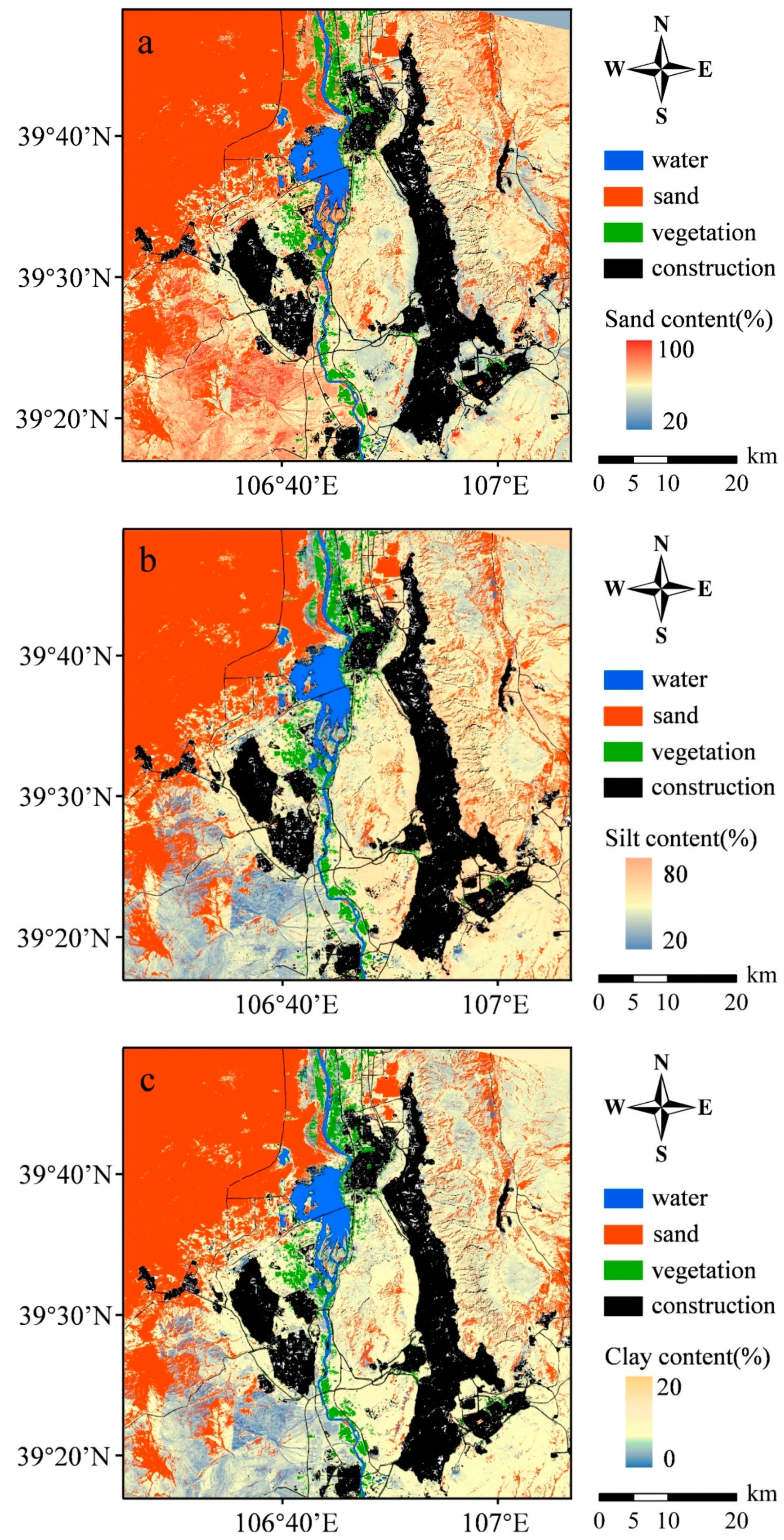
The 6SV-SVM model was used to predict the surface soil’s particle size content in the study area: the 6SV atmospheric correction was performed using RSD software to calculate the surface reflectance image of the entire study area, read the reflectance data of each image element, import the data into MATLAB software, use our 6SV-SVM model to calculate the sand, silt, and clay contents of each image element in the map, and export the data. The data were then added to ArcGIS software and overlaid with the classification layers of other feature types in the study area to obtain the inversion results of the soil grain size content (Figure 14). The northwest of the study area is a desert area, and the Yellow River in the middle meanders from south to north, with a small amount of vegetation on both banks. Except for urban buildings and mine construction land, the sand content of the bare land soil is high on the east and west sides and low in the middle. The desert border area in the northeast and southwest has a high sand content of about 70%. The area near the riverbank in the middle has a small increase of about 60%, and the rest is about 20–40% (Figure 14a). The distribution of the silt content is opposite to that of the sand content, which is low on the east and west sides and high in the middle. The silt content of the soil in the northeast and southwest is low, about 30%, and in other areas is about 60% (Figure 14b). The clay content is generally low, almost 0 in the northeast and southwest, and the overall average is about 11.25% (Figure 14c).

4. Discussion

4.1. Effectiveness of Surface Spectral Reflectance Data in Predicting Soil Particle-Size Distribution

Soil texture is an important physical property. Monitoring the soil particle-size distribution change during mine reclamation is a key indicator for evaluating the success or failure of ecological restoration in a mining area. Spectral characteristics, as an effective indicator to analyze gradual topsoil change, are affected by the difference of different particle sizes’ contents in soil. The grain size increase is accompanied by a decrease in the spectral reflectance in the visible and near-infrared bands. At present, remote sensing images of bare soil and the spectral reflectance of soil samples are successfully used to estimate soil properties accurately and quickly. However, the relationship between spectral reflectance and soil texture is affected by factors such as soil moisture and surface vegetation coverage. When it is used on a large scale from experimental testing to on-site use, the surface state change may lead to a large deviation in its accuracy.
In the arid and semi-arid opencast coal mine area in western China, the ecological restoration and topsoil reconstruction work for reclamation requires an effective method to dynamically monitor the surface soil particle size contents and distribution information. Its arid climate conditions and disturbance factors greatly reduce the influence of soil moisture and vegetation cover on soil texture monitoring using reflectance spectroscopy. In this study, the surface reflectance data from the Landsat8 OLI images are considered, and models are established in some research areas of Wuhai City, Inner Mongolia Autonomous Region, western China, to analyze different methods’ prediction accuracies for surface soil sand, silt, and clay particle sizes’ contents, and the inversion results are obtained by using the model calculation.

4.2. Evaluation of Advantages and Disadvantages of Different Models

The advantages and disadvantages of the two atmospheric correction methods for the Landsat8 OLI images were evaluated. The soil particle size content was modeled and analyzed using the surface reflectance data of the 6SV atmospheric correction, and the accuracy was better than that of the FLAASH atmospheric correction. Thus, the 6SV atmospheric correction model for the Landsat8 OLI images has better applicability in the study area. Considering the surface heterogeneity in the micro area and the combination of the high-spatial, -temporal, and -resolution meteorological auxiliary data, compared with the conventional FLAASH atmospheric correction model, it can truly reflect its surface reflectance characteristics.
The advantages and disadvantages of several statistical regression methods were evaluated to predict soil properties according to surface reflectance spectra characteristics. The results show that, although the single-band model selects the band data with the highest correlation coefficient, and the multi-band model adds some band data with low correlation, except for the multi-band FLAASH-PLSR model, the multi-band data model’s performance is better than the single-band data model’s. In addition, among the three single-band prediction models for the particle size content, the powder content prediction model with the highest accuracy does not have a significant prediction ability. One possible reason is that the single-band model lacks sufficient band information to solve the complex regression problem.
Generally, simple regression methods may be preferred for establishing prediction models. However, when the single feature band regression method cannot solve the regression prediction problem of soil particle size characteristics, the multivariable regression technology that is suitable for describing the complex relationship of the spectral characteristics becomes a very good alternative method. Among the multi-band data models, the SVM model has the best performance, followed by the MLR model, and the PLSR model has the worst performance. The MLR model directly establishes the linear regression relationship between multi-band surface spectral reflectance data and soil particle size content, while the PLSR model extracts the principal components of the surface spectral reflectance data and uses reduced-dimension data with original characteristics for ordinary least squares regression (OLSR). The SVM model is the opposite of the PLSR model. The original data are upgraded to effectively achieve nonlinear regression prediction in a high-dimensional space. Combining the original band data’s dimension difference with the three multi-band models’ performances, the model’s accuracy is shown to increase with the increase in the band data dimension, which may explain the difference in the three multi-band data models’ performances to some extent.
In addition, the better precision performance in the regression of the reflectance spectral data is not only due to the selection of the modeling methods but is also affected by the number of measured samples and sample range. Due to insufficient sample space coverage and other reasons, the soil particle size content prediction error may also be higher. The prediction value of the clay content in a small amount of soil samples in this study is negative, with large errors. If the sample range is expanded, the prediction result may be more accurate.

4.3. Applicability and Limitations

The 6SV-SVM topsoil particle size content prediction model based on the Landsat8 OLI images that were finally established in this paper is more effectively applied to arid and semi-arid climate regions with large topographic relief. The prediction accuracy R 2 of sand, silt, and clay particle size contents of 0–40 cm thick soil in this study area have reached more than 0.95, which helps study mine ecological restoration and soil reconstruction in arid and semi-arid regions in western China. It provides an effective method for dynamically monitoring the soil texture change information. In addition, the image data resolution used in this study is limited, and there is less soil sample data collected on the spot. In future research, conducting more field surveys, expanding the sample collection, and using drones and other remote sensing methods to carry out detailed research on the reclaimed soil in the mining area are necessary to improve the soil particle-size distribution prediction accuracy.

5. Conclusions

In this study, based on the texture change monitoring of reclaimed soil from arid and semi-arid mines in western China, using Landsat8 OLI multispectral images and measured soil sample particle-size data, the prediction method for sand, silt, and clay contents in topsoil was established using the surface reflectance calculation method, soil thickness correlation statistical analysis, and single-band and multi-band models. The results show that:
(1)
Compared with the FLAASH atmospheric correction model, the calculated surface reflectance data for modeling and analyzing the soil particle-size contents have higher accuracy and can more truly reflect its surface reflectance characteristics when using the 6SV atmospheric correction model in arid and semi-arid areas with undulating terrain;
(2)
Among the particle size content data of 3 kinds of soil with different thicknesses (0–20 cm, 0–40 cm, and 0–60 cm), the sand and silt contents of the soil with a thickness of 0–40 cm have the strongest correlation with the reflectance data of multiple bands, which is the optimum soil thickness for modeling and predicting the particle size content in this study;
(3)
The order of the single-band prediction model’s accuracy is silt > sand > clay. The adjusted R 2 values of the silt and sand content prediction models are 0.518 and 0.451, respectively, and the clay content model does not have significant prediction ability;
(4)
The order of the multi-band prediction model’s accuracy is SVM > MLR > PLSR. Among them, the 6SV-SVM model has the highest accuracy in predicting the particle size content of the soil with a thickness of 0–40 cm, and the prediction accuracy R 2 of the 3 particle sizes’ contents is above 0.95;
(5)
The 6SV-SVM model based on Landsat8 OLI images established in this study can calculate the soil particle size content distribution in arid and semi-arid areas with undulating terrain. It is suitable for arid and semi-arid mines in western China and other areas with complex terrain. It provides effective data support for the change monitoring of mine-reclaimed soil texture. It has broad application prospects in mastering the law of soil particle-size change and optimizing regional ecological environment governance monitoring.

Author Contributions

Conceptualization, Q.L. and Z.H.; methodology, Q.L. and F.Z.; software, Q.L. and Y.Y.; investigation, D.S.; resources, Y.L.; data curation, Q.L. and D.S.; writing—original draft preparation, Q.L.; writing—review and editing, Z.H.; visualization, Q.L.; supervision, Z.H.; project administration, Z.H.; funding acquisition, Y.L. All authors have read and agreed to the published version of the manuscript.

Funding

This research was funded by “the National Natural Science Foundation of China, grant number 41771542” and “the General Program of Beijing Natural Science Foundation, grant number 4202065”.

Data Availability Statement

Not applicable.

Acknowledgments

The authors thank the Institute of Land Reclamation and Ecological Reconstruction for their help in this research.

Conflicts of Interest

The authors declare no conflict of interest.

References

  1. Azizi, K.; Garosi, Y.; Ayoubi, S.; Tajik, S. Integration of Sentinel-1/2 and topographic attributes to predict the spatial distribution of soil texture fractions in some agricultural soils of western Iran. Soil Tillage Res. 2023, 229, 105681. [Google Scholar] [CrossRef]
  2. Bi, Y.L.; Peng, S.P.; Du, S.Z. Technological difficulties and future directions of ecological reconstruction in open pit coal mine of the arid and semi-arid areas of Western China. J. China Coal Soc. 2021, 46, 1355–1364. [Google Scholar] [CrossRef]
  3. Han, J.Z.; Hu, Z.Q.; Wang, P.J.; Yan, Z.G.; Li, G.S.; Zhang, Y.H.; Zhou, T. Spatio-temporal evolution and optimization analysis of ecosystem service value-A case study of coal resource-based city group in Shandong, China. J. Clean Prod. 2022, 363, 12. [Google Scholar] [CrossRef]
  4. Hu, Z.Q.; Zhao, Y.L. Main problems in ecological restoration of mines and their solutions. China Coal 2021, 47, 2–7. [Google Scholar] [CrossRef]
  5. Hu, Z.Q.; Zhao, Y.L. Principle and technology of coordinated control of eco-environment of mining areas and river sediments in Yellow River watershed. J. China Coal Soc. 2022, 47, 438–448. [Google Scholar] [CrossRef]
  6. Xi, J.P. Speech at the symposium on ecological protection and high-quality development in the Yellow River basin. Water Conserv. Constr. Manag. 2019, 39, 1–3+6. [Google Scholar] [CrossRef]
  7. Bao, N.; Liu, S.; Zhou, Y. Predicting particle-size distribution using thermal infrared spectroscopy from reclaimed mine land in the semi-arid grassland of North China. Catena 2019, 183, 104190. [Google Scholar] [CrossRef]
  8. Domínguez-Haydar, Y.; Velásquez, E.; Carmona, J.; Lavelle, P.; Chavez, L.F.; Jiménez, J.J. Evaluation of reclamation success in an open-pit coal mine using integrated soil physical, chemical and biological quality indicators. Ecol. Indic. 2019, 103, 182–193. [Google Scholar] [CrossRef]
  9. Clark, R.N.; Roush, T.L. Reflectance spectroscopy: Quantitative analysis techniques for remote sensing applications. J. Geophys. Res. Solid Earth 1984, 89, 6329–6340. [Google Scholar] [CrossRef]
  10. Xiao, J.; Shen, Y.; Tateishi, R.; Bayaer, W. Development of topsoil grain size index for monitoring desertification in arid land using remote sensing. Int. J. Remote Sens. 2007, 27, 2411–2422. [Google Scholar] [CrossRef]
  11. Ben-Dor, E.; Chabrillat, S.; Demattê, J.A.M.; Taylor, G.R.; Hill, J.; Whiting, M.L.; Sommer, S. Using Imaging Spectroscopy to study soil properties. Remote Sens. Environ. 2009, 113, S38–S55. [Google Scholar] [CrossRef]
  12. Fongaro, C.T.; Demattê, J.A.M.; Rizzo, R.; Lucas Safanelli, J.; Mendes, W.D.; Dotto, A.C.; Vicente, L.E.; Franceschini, M.H.D.; Ustin, S.L. Improvement of Clay and Sand Quantification Based on a Novel Approach with a Focus on Multispectral Satellite Images. Remote Sens. 2018, 10, 1555. [Google Scholar] [CrossRef]
  13. Shi, P.; Six, J.; Sila, A.; Vanlauwe, B.; Van Oost, K. Towards spatially continuous mapping of soil organic carbon in croplands using multitemporal Sentinel-2 remote sensing. ISPRS J. Photogramm. Remote Sens. 2022, 193, 187–199. [Google Scholar] [CrossRef]
  14. Wang, S.; Guan, K.; Zhang, C.; Lee, D.; Margenot, A.J.; Ge, Y.; Peng, J.; Zhou, W.; Zhou, Q.; Huang, Y. Using soil library hyperspectral reflectance and machine learning to predict soil organic carbon: Assessing potential of airborne and spaceborne optical soil sensing. Remote Sens. Environ. 2022, 271, 112914. [Google Scholar] [CrossRef]
  15. McCarty, G.W.; Reeves, J.B.; Reeves, V.B.; Follett, R.F.; Kimble, J.M. Mid-infrared and near-infrared diffuse reflectance spectroscopy for soil carbon measurement. Soil Sci. Soc. Am. J. 2002, 66, 640–646. [Google Scholar] [CrossRef]
  16. Chen, F.; Kissel, D.E.; West, L.T.; Adkins, W.; Rickman, D.; Luvall, J.C. Mapping soil organic carbon concentration for multiple fields with image similarity analysis. Soil Sci. Soc. Am. J. 2008, 72, 186–193. [Google Scholar] [CrossRef]
  17. D’Acqui, L.P.; Pucci, A.; Janik, L.J. Soil properties prediction of western Mediterranean islands with similar climatic environments by means of mid-infrared diffuse reflectance spectroscopy. Eur. J. Soil Sci. 2010, 61, 865–876. [Google Scholar] [CrossRef]
  18. Levi, N.; Karnieli, A.; Paz-Kagan, T. Airborne imaging spectroscopy for assessing land-use effect on soil quality in drylands. ISPRS J. Photogramm. Remote Sens. 2022, 186, 34–54. [Google Scholar] [CrossRef]
  19. Shoshany, M.; Roitberg, E.; Goldshleger, N.; Kizel, F. Universal quadratic soil spectral reflectance line and its deviation patterns’ relationships with chemical and textural properties: A global data base analysis. Remote Sens. Environ. 2022, 280, 113182. [Google Scholar] [CrossRef]
  20. Zolfaghari, A.A.; Toularoud, A.A.S.; Baghi, F.; Mirzaee, S. Spatial prediction of soil particle size distribution in arid agricultural lands in central Iran. Arab. J. Geosci. 2022, 15, 1574. [Google Scholar] [CrossRef]
  21. Shirazi, M.P.; Abtahi, S.A.; Nejad, M.B.; Moosavi, A.A.; Navidi, M.N. Improving Soil Texture Digital Mapping Using Landsat 8 Satellite Imageries in Calcareous Soils of Southern Iran. J. Agric. Sci. Technol. 2023, 25, 485–502. [Google Scholar]
  22. Zhao, X.; Xu, Z.J.; Yin, J.P.; Bi, R.T.; Feng, J.F.; Liu, P. Retrieval of Soil Organic Carbon in Cinnamon Mining Belt Subsidence Area Based on OLI and 6SV. Spectrosc. Spect. Anal. 2019, 39, 886–893. [Google Scholar]
  23. Madari, B.E.; Reeves, J.B.; Machado, P.; Guimaraes, C.M.; Torres, E.; McCarty, G.W. Mid- and near-infrared spectroscopic assessment of soil compositional parameters and structural indices in two Ferralsols. Geoderma 2006, 136, 245–259. [Google Scholar] [CrossRef]
  24. Liao, K.; Xu, S.; Wu, J.; Zhu, Q. Spatial estimation of surface soil texture using remote sensing data. Soil Sci. Plant Nutr. 2013, 59, 488–500. [Google Scholar] [CrossRef]
  25. Pereira, G.E.; Sequinatto, L.; Almeida, J.A.d.; ten Caten, A.; Mota, J.M. VIS-NIR spectral reflectance for discretization of soils with high sand content. Semin. Ciências Agrárias 2019, 40, 99–112. [Google Scholar] [CrossRef]
  26. Rosero-Vlasova, O.A.; Vlassova, L.; Pérez-Cabello, F.; Montorio, R.; Nadal-Romero, E. Soil organic matter and texture estimation from visible–near infrared–shortwave infrared spectra in areas of land cover changes using correlated component regression. Land Degrad. Dev. 2019, 30, 544–560. [Google Scholar] [CrossRef]
  27. Cooley, T.; Anderson, G.P.; Felde, G.W.; Hoke, M.L.; Ratkowski, A.J.; Chetwynd, J.H.; Gardner, J.A.; Adler-Golden, S.M.; Matthew, M.W.; Berk, A.; et al. FLAASH, a MODTRAN4-based atmospheric correction algorithm, its application and validation. In Proceedings of the IEEE International Geoscience and Remote Sensing Symposium, Toronto, ON, Canada, 24–28 June 2002; pp. 1414–1418. [Google Scholar]
  28. Houborg, R.; McCabe, M.F. Impacts of dust aerosol and adjacency effects on the accuracy of Landsat 8 and RapidEye surface reflectances. Remote Sens. Environ. 2017, 194, 127–145. [Google Scholar] [CrossRef]
  29. Escribano, P.; Schmid, T.; Chabrillat, S.; Rodríguez-Caballero, E.; García, M. Chapter 4—Optical Remote Sensing for Soil Mapping and Monitoring. In Soil Mapping and Process Modeling for Sustainable Land Use Management; Pereira, P., Brevik, E.C., Muñoz-Rojas, M., Miller, B.A., Eds.; Elsevier: Amsterdam, The Netherlands, 2017; pp. 87–125. [Google Scholar]
  30. Janik, L.J.; Forrester, S.T.; Rawson, A. The prediction of soil chemical and physical properties from mid-infrared spectroscopy and combined partial least-squares regression and neural networks (PLS-NN) analysis. Chemom. Intell. Lab. Syst. 2009, 97, 179–188. [Google Scholar] [CrossRef]
  31. Rossel, R.A.V.; Behrens, T. Using data mining to model and interpret soil diffuse reflectance spectra. Geoderma 2010, 158, 46–54. [Google Scholar] [CrossRef]
  32. Vereecken, H.; Schnepf, A.; Hopmans, J.W.; Javaux, M.; Or, D.; Roose, T.; Vanderborght, J.; Young, M.H.; Amelung, W.; Aitkenhead, M.; et al. Modeling Soil Processes: Review, Key Challenges, and New Perspectives. Vadose Zone J. 2016, 15, 1–57. [Google Scholar] [CrossRef]
  33. Zhang, F.; Hu, Z.Q.; Fu, Y.K.; Yang, K.; Wu, Q.Y.; Feng, Z.W. A New Identification Method for Surface Cracks from UAV Images Based on Machine Learning in Coal Mining Areas. Remote Sens. 2020, 12, 1571. [Google Scholar] [CrossRef]
  34. Zheng, G.; Ryu, D.; Jiao, C.; Xie, X.; Cui, X.; Shang, G. Visible and Near-Infrared Reflectance Spectroscopy Analysis of a Coastal Soil Chronosequence. Remote Sens. 2019, 11, 2336. [Google Scholar] [CrossRef]
  35. Tavakoli, H.; Correa, J.; Sabetizade, M.; Vogel, S. Predicting key soil properties from Vis-NIR spectra by applying dual-wavelength indices transformations and stacking machine learning approaches. Soil Tillage Res. 2023, 229, 105684. [Google Scholar] [CrossRef]
  36. Chursin, V.V.; Kuzhevskaia, I.; Merzliakov, O.E.; Valevich, T.; Ruchkina, K. Design of satellite sensing data classification algorithm based on machine learning using the example of granulometric composition of soils in agricultural landscapes of Western Siberia. Sovrem. Probl. Distantsionnogo Zondirovaniya Zemli Kosm. 2021, 18, 39–50. [Google Scholar] [CrossRef]
  37. Zhang, Y.; Zhang, L. Machine Learning Theory and Algorithms; Science Press: Beijing, China, 2012. [Google Scholar]
  38. Stevens, A.; van Wesemael, B.; Bartholomeus, H.; Rosillon, D.; Tychon, B.; Ben-Dor, E. Laboratory, field and airborne spectroscopy for monitoring organic carbon content in agricultural soils. Geoderma 2008, 144, 395–404. [Google Scholar] [CrossRef]
  39. Ishiyama, T.; Tsuchiya, K.; Sugihara, S. Ground surface features of the Taklimakan Desert. Adv. Space Res. 1996, 17, 41–48. [Google Scholar] [CrossRef]
  40. Lagacherie, P.; Baret, F.; Feret, J.B.; Netto, J.M.; Robbez-Masson, J.M. Estimation of soil clay and calcium carbonate using laboratory, field and airborne hyperspectral measurements. Remote Sens. Environ. 2008, 112, 825–835. [Google Scholar] [CrossRef]
  41. Seidel, M.; Vohland, M.; Greenberg, I.; Ludwig, B.; Ortner, M.; Thiele-Bruhn, S.; Hutengs, C. Soil moisture effects on predictive VNIR and MIR modeling of soil organic carbon and clay content. Geoderma 2022, 427, 116103. [Google Scholar] [CrossRef]
  42. Li, P.F.; Li, B.G. Study on some characteristics of evaporation of sand dune and evapotranspiration of grassland in Mu Us desert. J. Hydraul. Eng. 2000, 3, 25–30. [Google Scholar]
  43. Zhang, L. Research on Reservoir Water Depth Inversion and Water Area Extraction Based on Multi-Band Remote Sensing. Master’s Thesis, Inner Mongolia Agricultural University, Huhhot, China, 2018. [Google Scholar]
  44. Xiong, Y.; Li, Q.K. China Soil, 2nd ed.; Science Press: Beijing, China, 1986. [Google Scholar]
  45. USGS. Available online: https://earthexplorer.usgs.gov/ (accessed on 5 May 2022).
  46. Li, M.; Han, D.; Wang, X. Spectral Analysis Techniques and Their Applications; Science Press: Beijing, China, 2006. [Google Scholar]
  47. Rouse, J.W.; Haas, R.H.; Schell, J.A.; Deering, D.W. Monitoring vegetation systems in the Great Plains with ERTS. NASA Spec. Publ. 1974, 351, 309. [Google Scholar]
  48. Tanre, D.; Deuze, J.L.; Herman, M.; Santer, R.; Vermote, E. Second Simulation of the Satellite Signal in the Solar Spectrum, 6S: An overview. IEEE Trans. Geosci. Remote Sens. 2002, 35, 675–686. [Google Scholar]
  49. Vermote, E.; Justice, C.; Claverie, M.; Franch, B. Preliminary analysis of the performance of the Landsat 8/OLI land surface reflectance product. Remote Sens. Environ. 2016, 185, 46–56. [Google Scholar] [CrossRef]
  50. CSDN. Available online: https://blog.csdn.net/gordon3000/article/details/102911626 (accessed on 5 November 2022).
  51. Dalal, R.C.; Henry, R.J. Simultaneous Determination of Moisture, Organic Carbon, and Total Nitrogen by Near Infrared Reflectance Spectrophotometry. Soil Sci. Soc. Am. J. 1986, 50, 120–123. [Google Scholar] [CrossRef]
  52. Wold, S. The multivariate calibration problem in chemistry solved by the PLS method. In Lecture Notes in Mathematics; Springer: Berlin/Heidelberg, Germany, 1983. [Google Scholar]
  53. Hapke, B. Theory of Reflectance and Emittance Spectroscopy; Cambridge University Press: Cambridge, UK, 1993. [Google Scholar]
  54. Clark, R.N. Spectroscopy of rocks and minerals and principles of spectroscopy. Man. Remote Sens. 1999, 3, 3–58. [Google Scholar]
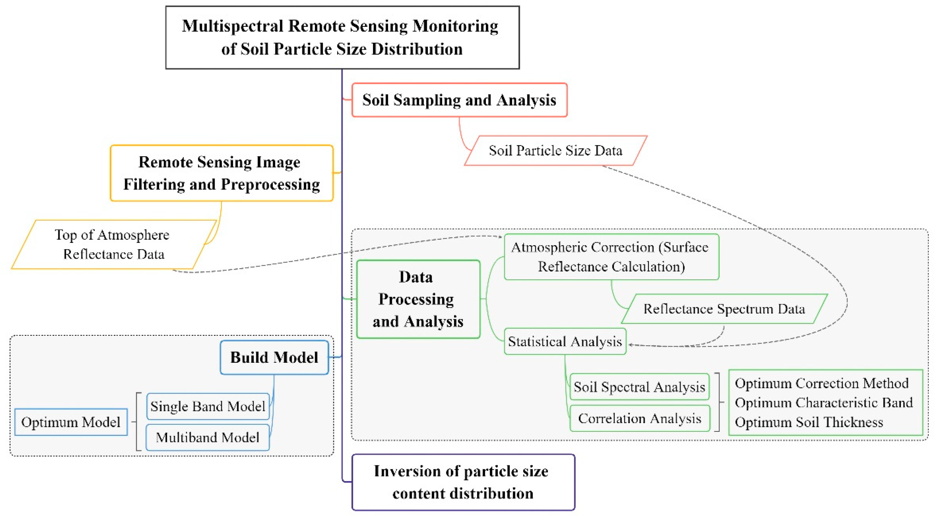
Figure 1. Experimental flow chart.
Remotesensing 15 02137 g001
Figure 2. (a) Overview map, (b) elevation change map, (c) NDVI distribution map, and (d) soil sampling distribution map of the study area.
Remotesensing 15 02137 g002
Figure 3. Photos of soil sampling.
Remotesensing 15 02137 g003
Figure 4. Histogram of soil particle-size distribution at sampling points with different soil layer thicknesses: (a) 0–20 cm, (b) 20–40 cm, and (c) 40–60 cm.
Remotesensing 15 02137 g004
Figure 5. Statistics histogram of NDVI values in the study area.
Remotesensing 15 02137 g005
Figure 6. Reflectance spectra of topsoil samples with different atmospheric correction models: (a) FLAASH atmospheric correction model and (b) 6SV atmospheric correction model.
Remotesensing 15 02137 g006
Figure 7. Correlation between soil particle-size content in different thickness and reflectance spectra of (a) FLAASH atmospheric correction model and (b) 6SV atmospheric correction model.
Remotesensing 15 02137 g007
Figure 8. Correlation between particle size content and reflectance spectra of 2 atmospheric correction models under 0–40 cm soil thickness.
Remotesensing 15 02137 g008
Figure 9. The quantile–quantile plots of (a) soil sand, (b) silt, and (c) clay content.
Remotesensing 15 02137 g009
Figure 10. Fitting effect of (a) MLR, (b) PLSR, and (c) SVM models, (I) sand, (II) silt, and (III) clay content predicted, and true values using FLAASH atmospheric correction surface reflectance data.
Remotesensing 15 02137 g010
Figure 11. Regression between predicted and true values of (a) MLR, (b) PLSR, and (c) SVM models, (I) sand, (II) silt, and (III) clay content using FLAASH atmospheric correction surface reflectance data.
Remotesensing 15 02137 g011
Figure 12. Fitting effect of (a) MLR, (b) PLSR, and (c) SVM models, (I) sand, (II) silt, and (III) clay content predicted and true values using 6SV atmospheric correction surface reflectance data.
Remotesensing 15 02137 g012
Figure 13. Regression between predicted and true values of (a) MLR, (b) PLSR, and (c) SVM models, (I) sand, (II) silt, and (III) clay content using 6SV atmospheric correction surface reflectance data.
Remotesensing 15 02137 g013
Figure 14. Inversion results of soil particle sizes’ contents (a) sand, (b) silt, and (c) clay.
Remotesensing 15 02137 g014
Table 1. Average content of soil particles at different sampling points.
Sampling PointSoil Thickness (cm)Average Content (%)
SandSiltClay
C0–2061.95436.8001.246
0–4066.11432.4671.419
0–6066.33932.1851.476
H0–2031.79860.2267.976
0–4024.07166.1679.763
0–6026.36163.9179.723
Table 2. Landsat8 OLI image band parameters.
BandWavelength Range/μm Signal-to-Noise Ratio Spatial Resolution/m
1—COASTAL/AEROSOL0.43–0.4513030
2—Blue0.45–0.5113030
3—Green0.53–0.5910030
4—Red0.64–0.679030
5—NIR0.85–0.889030
6—SWIR11.57–1.6510030
7—SWIR22.11–2.2910030
8—PAN0.50–0.688015
9—Cirrus1.36–1.385030
Table 3. Regression analysis of single-band optimum fitting model for three particle sizes.
Soil PropertiesOptimum Model FunctionR2FP
Sand contentExp2PMod20.45146.7051.199 × 10−5 *
Silt contentLangevin0.51871.4152.168 × 10−7 *
Clay contentExp1p2Md0.17217.0241
* At 0.05 level, the fitting equation is obviously better than the equation y = c o n s t a n t .
Table 4. Regression equation coefficient of MLR and PLSR models.
Model y i (Particle Size Content) b k 1 k 2 k 3 k 4 k 5 k 6 k 7
MLR y 1 (sand)−61.51−3.070.8436.91−7.91−1.659.26−19.92
y 2 (silt)111.97−6.809.59−20.32−1.540.45−4.9613.82
y 3 (clay)49.549.87−10.43−16.599.451.20−4.306.10
PLSR y 1 (sand)111.003.111.700.360.07−2.61−0.96−0.61
y 2 (silt)2.19−2.79−1.59−0.43−0.142.160.740.45
y 3 (clay)−13.20−0.32−0.110.070.080.450.220.16
Table 5. Prediction accuracy of MLR, PLSR, and SVM models.
Atmospheric Correction ModelModelEvaluation IndexSoil Properties
Sand ContentSilt ContentClay Content
FLAASHMLRR20.8560.7980.955
F5.9483.94321.102
PLSRR20.1380.0810.240
SVMR20.9460.9530.936
MSE0.0080.0080.008
6SVMLRR20.9340.8990.926
F14.1298.87312.435
PLSRR20.5910.6670.307
SVMR20.9580.9650.983
MSE0.0070.0060.003
Disclaimer/Publisher’s Note: The statements, opinions and data contained in all publications are solely those of the individual author(s) and contributor(s) and not of MDPI and/or the editor(s). MDPI and/or the editor(s) disclaim responsibility for any injury to people or property resulting from any ideas, methods, instructions or products referred to in the content.