Shoreline Detection from PRISMA Hyperspectral Remotely-Sensed Images

Abstract

Coastal managers, policymakers, and scientists use shoreline accretion/erosion trends to determine the coastline’s historical evolution and generate models capable of predicting future changes. Different solutions have been developed to obtain shoreline positions from Earth observation data in recent years, the so-called Satellite-Derived Shorelines (SDS). Most of the methodologies available in the literature use multispectral optical satellite imagery. This paper proposes two new methods for shoreline mapping at the subpixel level based on PRISMA hyperspectral imagery. The first one analyses the spectral signatures along defined beach profiles. The second method uses techniques more commonly applied to multispectral image analysis, such as Spectral Unmixing algorithms and Spatial Attraction Models. The results obtained with both methodologies are validated on three Mediterranean microtidal beaches located in two different countries, Italy and Greece, using image-based ground truth shorelines manually photointerpreted and digitised. The obtained errors are around 6 and 7 m for the first and second methods, respectively. These results are comparable to the errors obtained from multispectral data. The paper also discusses the capability of the two methods to identify two different shoreline proxies.

1. Introduction

The International Geographic Data Committee has recognised coastlines as one of the 27 most important features to map and monitor [1]. Coastal areas are the most populated areas [2], and they are increasingly vulnerable to erosion due to climate change, i.e., sea-level rise and more frequent extreme events [3,4]. Shoreline position and its variability have been used as an indicator in many coastal morphodynamic studies, and time series of shoreline position has been used to calculate rates of erosion/accretion [2,5] as beaches are natural protection for coastal areas as they act as a buffer for wave energy during storms, protecting the areas behind them from damage and flooding [6]. Various technologies are used to monitor and map the coastline (from field surveys to satellites). Among them, remote sensing techniques have stood out in the last decades for requiring less data acquisition time compared to traditional topographic surveys [7,8]. In this group of techniques, satellite remote sensing data are the most promising. Satellites provide images that cover large areas with high spatial and temporal resolutions, allowing near-real-time analysis of any point on Earth. Considering only the most widely used open-source constellations, Landsat (National Aeronautics and Space Administration, NASA) and Sentinel (European Commission through European Space Agency, ESA), medium spatial resolution images of the whole globe have been available since 1984 when Landsat-5 was launched. This satellite and its successors (Landsat 7–8) have a resolution of 30 m for the bands R, G, B, NIR, and SWIR-1, usually involved in the detection of the coastline, while Sentinel-2, the resolution is 10 m for the first four and 20 m for SWIR-1. The revisit times range between 5 and 16 days [9,10]. In recent decades, several algorithms and detection methodologies have been developed for automatic shoreline mapping from satellite remote sensing imagery (hereafter referred to as Satellite-Derived Shorelines, SDS). These algorithms are image-based models using image processing techniques. Two groups of satellites can be distinguished. First, synthetic aperture radar (SAR) satellites use microwaves to illuminate the target and record pulse echoes. The advantage of these satellites is that they produce images that can be used in adverse weather conditions (e.g., heavy cloud cover) and at any time of day (e.g., at night). These characteristics make SAR sensors a promising data source for developing coastal sensing applications for shoreline mapping [8,11]. On the other hand, multispectral (MSI) and hyperspectral (HSI) sensors record the response of targets at different wavelengths of the electromagnetic spectrum. To the best of the authors’ knowledge, two reviews collect information on the methods developed for the last type of satellites [12,13]. Both reviews collect and summarise the methodologies applied to MSI for shoreline detection. In contrast, HSI is barely mentioned. The main difference between the multi and hyperspectral images is the spectral and spatial resolution. While MSI usually has high spatial resolution and low spectral resolution, HSI has low spatial resolution and high spectral resolution. The HSI sensor measures contiguous wavelengths in narrow spectral bands (on the order of 10 nm), resulting in near-continuous spectral signatures that allow for better differentiation of materials and objects on the ground. However, due to high spectral resolutions, the images contain some “repeated” information; contiguous bands may not contain discriminant information between materials. Therefore, the algorithms initially developed to work with MSI are inefficient on HSI [14]. These limitations may be the reason for the scarcity of studies for obtaining the coastline using HSI [13]. Most studies combine HSI data with other sensors [15,16,17,18,19]; therefore, new solutions exploring the SDS obtained from HSI are needed. Recently, few papers have been published exclusively using HSI imagery. Ref. [20] propose a new method focused on shoreline detection on muddy coasts. This methodology uses Sentinel imagery; however, its applicability was tested on a hyperspectral image from the Advanced Hyperspectral Imager (AHSI) satellite. The steps for shoreline detection involve the selection of the optimal band (most significant reflectance difference between water and land) to which a high-pass filter is applied. From the resulting image, the range of reflectance values containing the low-frequency information is obtained by statistical histogram analysis. Finally, the image is binarised into land and water by a morphological filter using the range calculated above. Alternatively, ref. [21] use a Hyperion image in the Bosphorus area (Turkey) to determine the influence of Dimension Reduction (DR) methods to decrease the number of bands on shoreline extraction. The applied DR techniques were: (i) Principal Component Analysis, (ii) Maximum Noise Fraction and (iii) Independent Component Analysis. The bands obtained with each method are the inputs to classify the image, which is finally compared with the classified image using all the bands. Finally, ref. [22] present an algorithm developed on EO-1 Hyperion images. This method classifies images into four classes or features: water, vegetation, impervious and soil. Each class is represented by an index defined as a combination of the reflectance values of specific bands. Pixels with the highest index values are assigned to the class, and a reference spectrum is defined as its mean spectral signature. The PPI algorithm [23] is then used to identify a set of “pure” spectral signatures, often referred to as endmembers, so that the signature of each pixel can be expressed as a linear combination of them. These are assigned to the classes defined above by calculating the corresponding spectral angles. The “endmembers” abundances for each pixel are used as input for the Spatial Attraction Model (SAM) [24], in which every pixel is divided into sub-pixels.

The Italian Space Agency launched the hyperspectral Earth observation satellite mission called “PRecursore IperSpettrale della Missione Applicativa” (hereafter PRISMA) on 22 March 2019, by flight VEGA VV14 [25]. This satellite, which has a scheduled operational lifetime of five years, follows a Sun-synchronous orbit flying at an altitude of 615 km and with an inclination of 97.851 degrees. The revisit time of the satellite is 29 days, but the revisit capability is reduced to seven days by considering off-nadir angles. The satellite acquires images on demand according to “user’s needs” [26]. The images are available free of charge and can be downloaded from 21 May 2020, from https://www.asi.it/scienze-della-terra/prisma/, (accessed on 14 January 2023) after the user’s registration. The mission parameters are summarised in

Table 1. Main PRISMA mission characteristics.

Orbit altitude reference	615 km
Lifetime	5 years
Revisit time	29 days
Relook time	7 days

.

One of the main objectives of PRISMA is to support the development of new applications and algorithms for environmental monitoring and resource management [25]. Since PRISMA’s imagery has become widely available, many studies have been developed taking advantage of this new technology and related to different applications such as water [27,28], vegetation [29,30] or fire detection [31].

This publication aims to develop new solutions for SDS mapping, taking advantage of the new Italian HSI satellite PRISMA. The newly developed algorithms are referred to hereafter as “Method I: profiles approach” and “Method II: k-means approach”. Both methods have been tested on three different sites located in the Mediterranean Sea: Poetto (Sardegna, Italy), Ostia (Lazio, Italy) and Kolymvari (Crete, Greece). The accuracy of the obtained SDS is finally estimated using digitised shorelines on (almost) synchronous satellite images as image-based ground truth data (hereafter GT shorelines). The (almost) synchronous images used are Sentinel-2, Landsat 7 and 8, and very high-resolution Pleiades images. The last ones were made available for this study through the Data Warehouse Mechanisms of ESA in the framework of the H2020 ECFAS project (A proof of concept for the implementation of a European Copernicus coastal flood awareness system, GA n° 101004211, https://www.ecfas.eu/, accessed on 14 January 2023). Given the importance of shoreline analysis for coastal management purposes and in the aftermath of storm events that could generate large erosion impact, the ECFAS project aimed at developing tools and products for the evolution of the Emergency Management Service of Copernicus (CEMS), exploiting the medium resolution images from Landsat and Sentinel constellations to analyze shoreline displacement on low-lying coasts due to storm events using the semi-automatic algorithm for SDS extraction developed in the project, the Shoreline Analysis and Extraction Tool—SAET [32]. ECFAS has demonstrated that shoreline analysis can become an added-value product in the CEMS mapping component (https://emergency.copernicus.eu/mapping/, accessed on 14 January 2023) for emergency response and recovery actions.

2. Materials and Methods

2.1. PRISMA Mission and Products, HSI and PAN

The PRISMA payload, i.e., the elements producing the images, is constituted by a panchromatic camera that captures in the 400 to 700 nm range and a Hyper-Spectral Imager, capable of capturing images in narrow spectral bands ranging from 400 to 2500 nm. Hence, each PRISMA image, covering 30 km × 30 km scenes, is composed of a hyperspectral image or HSI and a panchromatic image (PAN). In addition, each HSI is composed of two “sub cubes”: the visible near-infrared (VNIR) and the shortwave infrared (SWIR, see

Table 2. Main PRISMA products’ technical features.

	HSI-VNIR	HSI-SWIR	PAN
Swath (km)	30	30	30
Spatial resolution (m)	30	30	5
Spatial pixels	1000	1000	6000
Spectral range (nm)	400–1010	920–2500	400–700
Spectral bands	66	176	1
Spectral Sampling Interval, SSI (nm)	7.2–11	6.5–11	-
Spectral Resolution (nm)	9–13	9–14.5	-
Absolute Radiometric Accuracy	$⩽5\%$ (Stability $⩽\pm 1\%$)	$⩽5\%$ (Stability $⩽\pm 1\%$)	-

).

PRISMA delivers data in three product levels (Table 2, for product levels and data details, see [33]). Here, we use only the products of the highest level, which represent the bot-tom-of-atmosphere reflectance after applying the atmospheric correction [34]. All the products are geocoded and provided in the Hierarchical Data Format Release 5 (HDF5).

2.2. Shoreline Extraction Algorithms

Two different approaches for SDS retrieval have been developed and are introduced below. Before using the two approaches, a series of steps must be applied to the PRISMA images:

• Reflectance. The (at-surface) reflectance values (for VNIR, SWIR and PAN) are obtained from the respective “digital numbers” (n, unsigned 16-bit integers, which are provided by PRISMA) via linear transformation [33].

  $$R^c\left(n\right)=R_{\min }^c+\frac{R_{\max }^c-R_{\min }^c}{2^{16}-1}n$$

  (1)

  where $R_{min}^c$ and $R_{max}^c$ are the minimum and maximum scaling factor values which are specified inside the image file. Provided that $0\le n\le 2^{16}-1$, the reflectance values $R^c$ range from $R_{min}^c$ to $R_{max}^c$.
• Pansharpening methods use a multispectral image and a panchromatic band to obtain a new multispectral image with the spatial resolution of the panchromatic band [35]. Among the existing algorithms, the Gram–Schmidt adaptive method [35,36] is chosen since its low computational complexity reduces the spectral distortion produced by other algorithms while maintaining spatial information. Still, pansharpening is the most time-consuming step in the preprocessing, its computational cost increasing linearly with the size of the area.
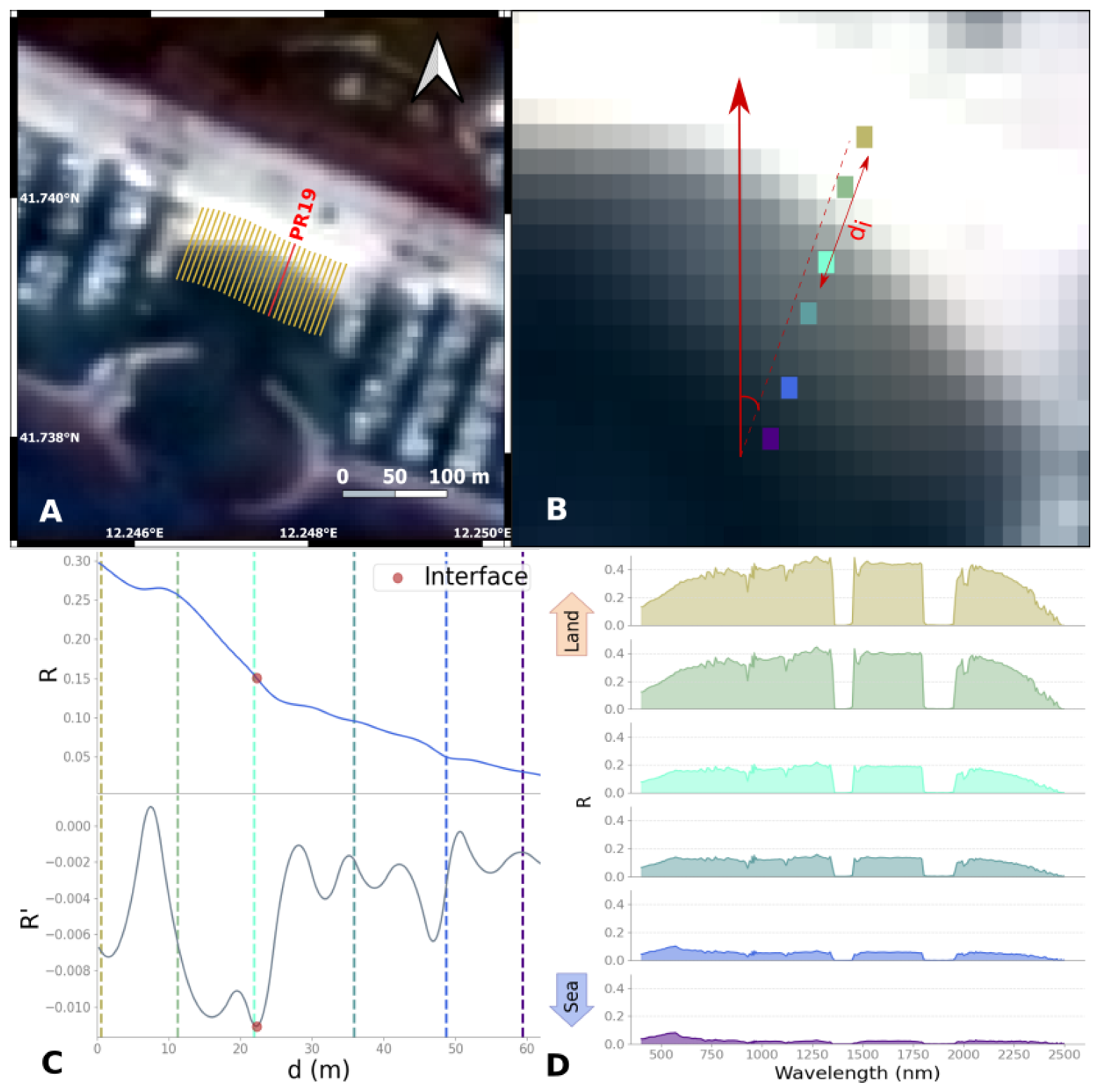
• Baseline and profiles. The baseline, i.e., the line delimiting the beach at its land part, is manually digitised from the pan-sharpened images of 5 m spatial resolution Area of Interest (AoI, Figure 1, insight B) and is then interpolated every 4.5 m to have at least one baseline point per pixel. Then, one profile per point is generated perpendicular to the baseline average direction (so that all the profiles are parallel).

The methodology and the inputs and outputs are represented in Figure 1.

2.2.1. Method I: Profile Approach

This method aims to detect the transition from sand to water by finding, for each profile, the point where the decrease (departing from the baseline) of the band-averaged reflectance values occurs faster. The method uses pan-sharpened AoI images of 5 m resolution (Figure 1B). The underlying principle is the different responses of water and sand. It is well known that water absorbs most of the NIR; therefore, the reflectance in these wavelengths is almost null. On the other hand, dry soil and land reflect more in all the wavelengths, especially in the NIR. The spectral signatures of the pixels that are crossed by the profiles were analysed to detect the differences between the signatures of the water pixels and those corresponding to other features (Figure 2B,D). The profiles approach has been used previously in other remote sensing coastal works using different types of data, for example, video monitoring [37] and satellite radar images [38]. Transects perpendicular to the beach shoreline are commonly used in shoreline displacement studies.

A profile going from $x^0$ to $x^F$ overlaps with n pixels, defining n segments (the part of the profile within the pixel) with midpoints $m^1,\dots ,m^n$.

Let $s\left(p\right)$ be the euclidean distance between $x^0$ and a point p on the profile,

$$s\left(p\right)=\sqrt{{\left(x^0-s\right)}^2}=\sqrt{{(x_x^0-s_x)}^2+{(x_y^0-s_y)}^2}$$

(2)

and $R^j$ the reflectance (averaged over all bands) of the pixel where $m^j$ falls into. Then we can use a cubic interpolation to calculate a function $R\left(s\right)$ from the n pairs $\{s\left(m^j\right),R^j\}$, representing the reflectance along the profile. An estimate of the interface point’s position $x^I$ is then obtained by minimizing the derivative

$$x^I={\mathrm{argmin}}_{x\in \mathrm{profile}}\frac{dR\left(s\right(x\left)\right)}{ds}$$

(3)

i.e., by finding the point where R decreases fastest.

This procedure is applied to each profile (Figure 2A), and the resulting set of points constitutes the ${\mathrm{SDS}}_{\mathrm{profile}}$.

2.2.2. Method II: k-Means Approach

Method II is a modification of the methodology proposed by [22], and it is applied to the 5 m spatial resolution pan-sharpened images cropped to the domain that strictly includes the profiles described in Method I (Figure 1C). In the following section, the different steps (Figure 3) used in the k-means approach are described. First, the unsupervised k-means algorithm implemented in the Python package spectral is applied to the spectral signatures of the pixels to cluster them into the classes. The k-means algorithm requires as input the desired number of clusters, which was set to three: water, sand and wet sand. Following the terminology of related works [39], the centroids of the clusters are considered in the following steps as the “endmembers” representing each class (Figure 3A).

The pixels usually contain more than one class/material. Therefore, the next step is to determine the abundance of each of the three endmembers for each of the pixels of the domain. Fully Constrained Least-Squares Based Linear Unmixing (FCLS) technique implemented in the pysptools Python package [38] has been used to get the three fraction maps. This technique assumes that each image pixel is constituted by the linear mixture of the (three) endmembers present in the image, and the fraction maps satisfy two constraints: (a) the sum of the abundances (fractions) sum up to one at each pixel and (b) all the abundances are non-negative. Once the abundances (fractions) maps are obtained (Figure 3B), the Spatial Attraction Model (SAM) described in [24] is applied to convert the above three fraction maps into one single class map (a segmented image with the dominant endmembers) at the subpixel level (Figure 3(C1)). SAM includes two user-defined parameters: the scale factor, S, which determines the number of sub-pixels present in the original pixel ($S^2$), and the neighbouring (quadrant, touching and surrounding). Each pixel (“parent pixel”) is divided into $S^2$ sub-pixels, with the abundances determining how many sub-pixels are to be assigned to each class (the higher the abundance of a class, the higher the number of sub-pixels for that class). Then, the location of the sub-pixels of each class within the parent pixel is determined according to the abundance fractions of neighbouring pixels, i.e., the abundance fractions of neighbours “attract” the sub-pixels of the same class. In this work, to obtain the highest number of subpixels, we consider $S=4$, resulting in class maps with a spatial resolution of 1.25 m and the neighbouring “quadrant”, which establishes that the pixels that can be considered neighbours of certain sub-pixels are in the same quadrant regarding the centre of the parent pixel. Next, a Sobel filter is applied to find the boundaries, both upper (border between wet and dry sands, in red in Figure 3(C3)) and lower (border edge between wet sand and water classes, in purple in Figure 3(C3)). Finally, two filters are applied to avoid artefacts: first, to remove the points of the edges that are more than two subpixels away from any of the two classes they delimit. A graph is then constructed in which the nodes are the points of the border, linking each pair of points whose distance is less than two subpixels and discarding all the points that are not in the largest connected component. In this way, two SDS are obtained from this method: the ${\mathrm{SDS}}_{\mathrm{upper}}$ and the ${\mathrm{SDS}}_{\mathrm{lower}}$.

2.3. Study Areas

A total of four beaches were selected in the Mediterranean Sea at three different sites and from two different countries to validate the shoreline detection algorithms proposed in this work. Three of these beaches are in Italy, and one is in Greece (Figure 4 upper panel). The Italian beaches are Poetto Beach in Sardinia (Figure 4A), Port Ostia Beach and Lido di Ostia Beach in the Lazio region (Figure 4B, green and red squares, respectively, in the same site). The Greek beach is Kolymvari, in the prefecture of Chania in Crete (Figure 4C, blue square). Two factors limited the selection of beaches: they had to be locations where the PRISMA satellite acquires images, and there had to be overlapping overpasses between PRISMA and other missions. Poetto is an 8 km long urban beach located on the Eastern part of Cagliari Gulf that preserves its natural state [40] (Figure 4A). It is a micro-tidal beach with tidal ranges lower than 20 cm [41,42]. Given the extent of the beach, four areas of interest were selected where SDS will be obtained (hereafter Poetto 1 to Poetto 4, from East to West, see Figure 4A. This beach presents the advantage that several PRISMA images were recorded concurrently with Open-Source satellite images (e.g., Sentinel-2 and Landsat 7-8).

Port Ostia Beach (hereafter “PortBeach”) and Lido di Ostia (“Ostia”) are urban beaches located in Rome’s coastal area (Figure 4B). The latter is part of the 20∼km long sandy beach forming the littoral extending south of the Tiber Delta. This stretch of coast is interrupted by a touristic harbour [43] where Port Ostia Beach is located. Here the local tide ranges are lower than 50 cm [44].

Finally, Kolymvary is an urban beach of 4 km in Chania that has suffered from erosion after the port construction in 2000 (Figure 4C). Local sources reported that the beach decreased its width from 50 to 25 m in two years, with the area next to the port (where the algorithms were tested) the narrowest zone [45]. The tidal range does not exceed ∼10 cm in this area [46].

2.4. PRISMA Dataset and Ground Truthing

The PRISMA image dataset employed in this study includes 7 images (

Table 3. Concurrent overpasses of PRISMA with medium and high-resolution satellite images used to digitise the shorelines, the image-based GT.

	PRISMA	Ground Truth (GT)
Beach	Overpass	Overpass	Mission	Resolution (Meters)
Poetto	2020/09/10 10:18:13	2020/09/10 10:20:01	Sentinel S2	10
	2020/10/09 10:17:51	2020/10/09 10:00:41	Landsat L8	15
	2021/02/14 10:22:50	2021/02/14 10:00:26	Landsat L8	15
	2021/05/12 10:21:40	2021/05/12 10:06:05	Landsat L8	15
	2021/05/29 10:15:00	2021/05/29 09:07:07	Landsat L7	15
PortBeach & Ostia	2020/08/06 10:14:13	2020/08/06 10:16:25	Pleiades PH1A	0.5
Kolymvari	2020/11/15 09:18:18	2020/11/15 09:02:26	Pleiades PH1B	0.5

) that met the requirements of being concurrent with other satellite missions and were free of clouds, which are known to affect the SDS mapping process [47]. In all the PRISMA images used, no foam is generated by the breaking waves, except in the Kolymvari scene.

Table 3 also includes information relative to the images used to assess the quality of proposed SDS algorithms. This study uses the well-known open-source mid-resolution missions Sentinel and Landsat for Poetto Beach and very high-resolution images from Pleaides, available through the ECFAS Project, for Ostia and Kolymvari beaches. Landsat and Sentinel images were downloaded using the Google Earth Engine API for Python, while the Pleiades images were obtained from the Copernicus Panda Catalogue (https://panda.copernicus.eu/, accessed on 14 January 2023). By selecting almost concurrent images (the maximum time interval is one hour, Table 3) and being in micro-tidal areas, tidal corrections were not performed, as done in previous works [48]. Two expert operators digitised the shorelines using the images from the concurrent missions (User I and User II in Figure 5). The shorelines were digitised twice to account for the errors made by the visual interpretation of the shoreline.

2.5. Georeferecing Accuracy and Co-Registration

The geolocation errors of the PRISMA products used in this work are estimated to be limited to 15 m if the images are provided after correction using Ground Control Points (GCPs) and to 200 m otherwise [49,50]. A recent study by [51] warns about GCPs not being operational at the time of image acquisition, which could explain why the observed offsets in the present study’s dataset are often larger than 15 m. These errors are too high for shoreline studies since they are in the order of magnitude of the variations analysed. In addition, the images used as GT also have geo-location errors of approximately 12 m [52,53]. Therefore, “co-registration” of the images is mandatory to properly assess the results of the proposed algorithms properly. For each pair of images, a set of pairs of analogous pixels (i.e., corresponding to the same features) were detected in each image to obtain information from one to another. The general perspective relationship between the two images is given by a homography [54]. Being $\left(c_{\mathrm{P}},r_{\mathrm{P}}\right)$ the pixel coordinates (column, row) in the PRISMA image and $\left(c_{\mathrm{GT}},r_{\mathrm{GT}}\right)$ the corresponding coordinates in the GT image frame, the homography relationship reads

$$\begin{array}{ccc}\hfill c_p=\frac{H_{11}{c}_{GT}+H_{12}{r}_{GT}+H_{13}}{H_{31}{c}_{GT}+H_{31}{r}_{GT}+1},& \hfill & \hfill r_p=\frac{H_{21}{c}_{GT}+H_{22}{r}_{GT}+H_{23}}{H_{31}{c}_{GT}+H_{32}{r}_{GT}+1}\end{array}$$

(4)

where $H_{ij}$ are the 8 parameters defining a homography from one frame to the other. However, provided that the images correspond to the “far field” (the satellite is very far away compared to the domain of the images), it can be assumed that $H_{31}\sim H_{32}\sim 0$ so that

$$\begin{array}{ccc}\hfill c_p=H_{11}{c}_{GT}+H_{12}{r}_{GT}+H_{13},& \hfill & \hfill r_p=H_{21}{c}_{GT}+H_{22}{r}_{GT}+H_{23}\end{array}$$

(5)

Provided a set of n ($\sim 10$ here) pairs between two images, the coefficients can be obtained by solving the system

$$\left(\begin{array}{cccccc}{c}_{\mathrm{GT},1}& r_{\mathrm{GT},1}& 1& 0& 0& 0\\ 0& 0& 0& c_{\mathrm{GT},1}& r_{\mathrm{GT},1}& 1\\ ⋮& ⋮& ⋮& ⋮& ⋮& ⋮\\ c_{\mathrm{GT},n}& r_{\mathrm{GT},n}& 1& 0& 0& 0\\ 0& 0& 0& c_{\mathrm{GT},n}& r_{\mathrm{GT},n}& 1\end{array}\right)·\left(\begin{array}{c}{H}_{11}\\ H_{12}\\ H_{13}\\ H_{21}\\ H_{22}\\ H_{23}\end{array}\right)=\left(\begin{array}{c}{c}_{\mathrm{P},1}\\ r_{\mathrm{P},1}\\ ⋮\\ c_{\mathrm{P},n}\\ r_{\mathrm{P},n}\end{array}\right).$$

(6)

While $n=3$ would suffice to solve for the three unknowns, a higher value was considered to assess the quality of the obtained transformation. Provided that the system is over-determined, the approximate solution ${\widehat{H}}_{ij}$ is found through the pseudo-inverse of the left-hand side matrix. The final error (Root Mean Squared Error, RMSE) of the transformation, expressed in pixels of the PRISMA image, is

$$\mathrm{RMSE}\left[\mathrm{pixel}\right]=\sqrt{\frac{1}{n}\sum _i^n\left[{\left(c_{\mathrm{P},i}-{\widehat{c}}_{\mathrm{P},i}\right)}^2+{\left(r_{\mathrm{P},i}-{\widehat{r}}_{\mathrm{P},i}\right)}^2\right]},$$

(7)

where $\left({\widehat{c}}_{\mathrm{P},i},{\widehat{r}}_{\mathrm{P},i}\right)$ are the reprojected coordinates given by

$$\left(\begin{array}{c}{\widehat{c}}_{\mathrm{P},1}\\ {\widehat{r}}_{\mathrm{P},1}\\ ⋮\\ {\widehat{c}}_{\mathrm{P},n}\\ {\widehat{r}}_{\mathrm{P},n}\end{array}\right)=\left(\begin{array}{cccccc}{c}_{\mathrm{GT},1}& r_{\mathrm{GT},1}& 1& 0& 0& 0\\ 0& 0& 0& c_{\mathrm{GT},1}& r_{\mathrm{GT},1}& 1\\ ⋮& ⋮& ⋮& ⋮& ⋮& ⋮\\ c_{\mathrm{GT},n}& r_{\mathrm{GT},n}& 1& 0& 0& 0\\ 0& 0& 0& c_{\mathrm{GT},n}& r_{\mathrm{GT},n}& 1\end{array}\right)·\left(\begin{array}{c}{\widehat{H}}_{11}\\ {\widehat{H}}_{12}\\ {\widehat{H}}_{13}\\ {\widehat{H}}_{21}\\ {\widehat{H}}_{22}\\ {\widehat{H}}_{23}\end{array}\right).$$

(8)

The RMSE can be alternatively expressed in meters provided by the resolution of the image.

3. Results

The errors associated with image co-registration and manual digitisation of shorelines by the two users are first shown and analysed. These errors assess the quality of the GT data. Then, the two proposed SDS approaches are compared with the image-based GT.

3.1. Ground Truth Error Assessment

3.1.1. Co-Registration Error

Table 4. Root Mean Square Error (RMSE) obtained for the homographies.

Beach	Date	♯ of Pairs	RMSE [m]
Poetto	10 September 2020	17	3.1
	9 October 2020	7	3.3
	15 October 2020	8	3.2
	14 February 2021	31	5.8
	12 May 2021	19	5.3
	29 May 2021	5	5.7
PortBeach & Ostia	6 August 2020	18	2.3
Kolymvari	15 November 2020	20	3.7

shows the number of pairs of features identified to co-register each image and the RMSE (expressed in m) obtained through the affine transformation as defined in Section 2.5.

The RMSE ranges between 2.3 m and 5.8 m, i.e., less than 1.5 pixels of the panchromatic image and, therefore, allows subpixel precision considering that the spatial resolution of PRISMA images is 30 m per pixel.

3.1.2. Manual Digitization Error

Two expert operators manually digitised the shorelines. In this work, the shoreline proxy used is the instantaneous shoreline described in [55], i.e., the interface between water and sand observed in the image. The error associated with the shoreline’s manual interpretation can represent a significant source of error [56,57]. For this purpose, for each beach and date, the distances between each point of User I to the polyline joining the points digitised by User II were calculated, following the methodology described in [58]. The distances are given with a sign, so they are positive/negative if the point of User I is seaward/landwards the polyline of User II.

Figure 6 shows the RMSE (Figure 6A) and bias (i.e., average, Figure 6B) values for all 23 shorelines digitised by both users. The digitised shorelines are generally very similar, with RMSE ranging from 0.9 to 10.23 m. The errors and biases at Poetto are larger than those obtained at Ostia and Kolymvari: this behaviour is related to the resolution of the images used as GT (Table 3). Considering the values in Table 4, both RMSE and bias are at the sub-pixel level for the GT image (and hence for the PRISMA image). Moreover, the User I shorelines are generally slightly biased seaward to the User II shorelines (positive biases).

Table 5. Time-averaged RMSE and bias in meters resulting from the user-digitized shoreline comparison per site.

Beach	RMSE [m]	Bias [m]
Poetto	6.4	+5.36
PortBeach & Ostia	1.20	−0.23
Kolymvari	1.98	−0.07

shows the time-averaged RMSE and bias per site.

Since the GT shorelines can be considered equivalent, for simplicity in the exposition of the results, the validation of the results will be done with the User I GT shorelines. Therefore, this GT shoreline will have an inherent error resulting from uncertainties in the image geolocation (georeferencing error, Table 4) and those associated with the digitising process (inter-operator errors, Table 5). The largest of which is the inherent error transmitted to the image validation process; 6 m in the case of Poetto Beach and 3 m for the other beaches. Consequently, any SDS obtained with the method presented here, profiles and k-means, will have associated the correspondent uncertainty.

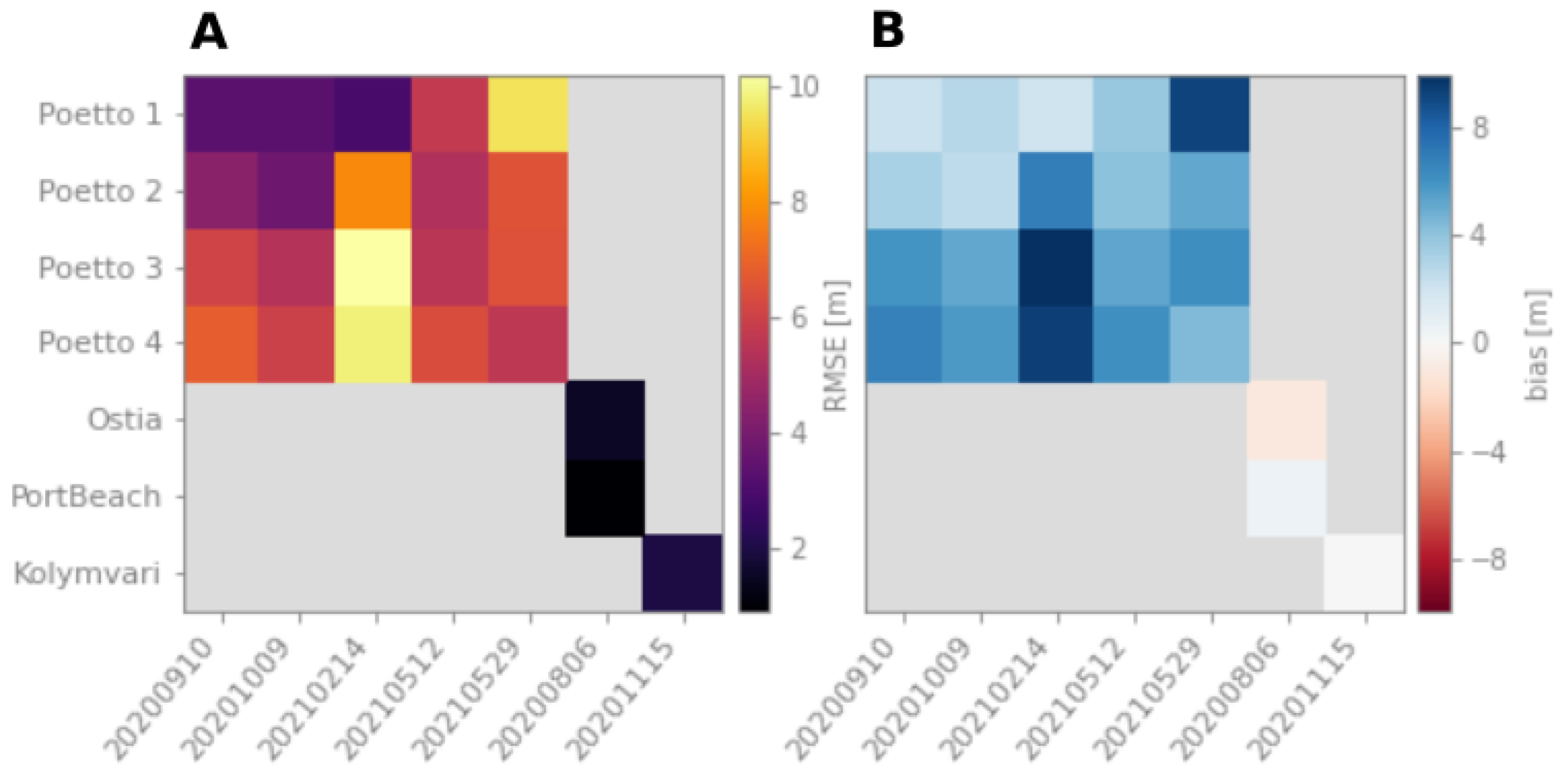
3.2. Method I: Profiles Approach Performance

The profiles approach was evaluated by comparing the 23 ${\mathrm{SDS}}_{\mathrm{profile}}$ with the two User I - GT shorelines. The RMSE and bias are calculated as described in Section 3.1.2, but in this case, the distances are computed from the ${\mathrm{SDS}}_{\mathrm{profile}}$ points to the digitized shorelines.

Figure 7 shows the RMSE (A) and bias (B) obtained by comparing the ${\mathrm{SDS}}_{\mathrm{profile}}$ with the GT shorelines. Errors for all beaches and dates range from 4 to 10 m, except for Kolymvari. A predominance of a seaward bias (positive values) of the GT shorelines with respect to the ${\mathrm{SDS}}_{\mathrm{profile}}$ is observed for almost all sites and beaches. In addition,

Table 6. Time-averaged RMSE and bias resulting from the comparison between the User GT shorelines and ${\mathrm{SDS}}_{\mathrm{profile}}$ comparison.

Beach	RMSE [m]	Bias [m]
Poetto	6.94	+2.65
PortBeach & Ostia	5.85	+0.81
Kolymvari	12.25	−10.03

shows the averaged values of RMSE and bias over time and AoI. Most importantly, except for Kolymvari, RMSEs are comparable to the GT inherent error.

The influence of profile direction on the method’s capability to retrieve the shoreline position was assessed in the $90\pm {15}^{\circ }$ range, finding errors lower than 5 m in Poetto beach for all the dates (Figure 8). The Method I profiles were robust, generating RMSE at the subpixel level even if the profile direction varies.

3.3. Method 2: k-Means Approach Performance

The performance of the k-means method is assessed by comparing the 23 shorelines obtained with this method (23 ${\mathrm{SDS}}_{\mathrm{upper}}$ and 23 ${\mathrm{SDS}}_{\mathrm{lower}}$) with the GT shorelines. Figure 8 shows the RMSE and bias of both limits (“upper” and “lower”) relative to the GT, and

Table 7. Time-averaged RMSE and bias resulting from the GT shorelines and ${\mathrm{SDS}}_{\mathrm{upper}}$ and ${\mathrm{SDS}}_{\mathrm{lower}}$ comparison.

	Beach	RMSE [m]	Bias [m]
${\mathrm{SDS}}_{\mathrm{upper}}$	Poetto	5.99	−2.61
	PortBeach & Ostia	3.19	+2.28
	Kolymvari	13.02	−0.12
${\mathrm{SDS}}_{\mathrm{lower}}$	Poetto	9.99	+9.45
	PortBeach & Ostia	15.95	+15.65
	Kolymvary	19.69	+14.35

summarises the results (time averaging).

From the values of RMSE in the Figure 8 and Table 7, ${\mathrm{SDS}}_{\mathrm{upper}}$ works notably better than ${\mathrm{SDS}}_{\mathrm{lower}}$, with errors that, except for Kolymvari, are similar to the inner errors of the GT. The bias performance is also better, in terms of absolute value, for the “upper” solution, working surprisingly well for Kolymvari.

4. Discussion

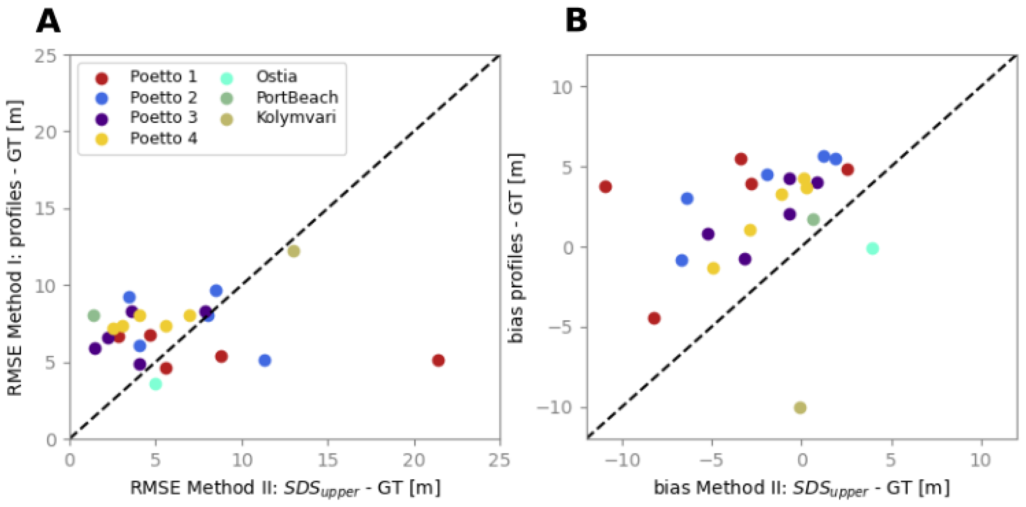
4.1. Profiles vs. k-Means Approaches

The performance of each methodology was determined by comparing their corresponding errors (relative to the image-based GT shoreline, i.e., as presented in Section 3.2 and Section 3.3).

Table 8. Time and beach averaged RMSE and bias for each of the presented methodologies, for all the AoI (Foam) and without the AoI with foam (No Foam).

	Foam		No Foam
	RMSE [m]	Bias [m]	RMSE [m]	Bias [m]
${\mathrm{SDS}}_{\mathrm{profile}}$	7.07	+1.94	6.98	+2.06
${\mathrm{SDS}}_{\mathrm{upper}}$	6.05	−2.08	5.77	−2.46

shows the averaged RMSE and bias for each method, while Figure 9 (A, B) shows the scatter plots of RMSE and bias, respectively, considering all dates and beaches. In the case of Method II, k-means, the results are presented considering the ${\mathrm{SDS}}_{\mathrm{upper}}$, as it has the lowest errors (Figure 9B,D). According to Table 8 and Figure 10, Method II seems to behave slightly better in terms of RMSE and bias than Method I; however, the differences are ∼1 m considering the mean values. Consequently, no significant improvements are obtained with Method II in terms of these two parameters.

The main difference between the two methods presented in this paper is the spectral information used to map the shoreline. While Method I uses the values resulting from averaging the reflectances of the different bands, Method II uses all the spectral information of the area of interest in the image. Since the Method I algorithm searches for the maximum slope of the derivative of the reflectance values averaged over the profiles, it will only detect one point per profile, so a unique SDS (${\mathrm{SDS}}_{\mathrm{profile}}$ in blue in Figure 11) is obtained. In contrast, Method II uses all the spectral signatures of the pixels to classify the image into three classes (water, wet sand, dry sand); consequently, two shorelines representing different interfaces are obtained (${\mathrm{SDS}}_{\mathrm{upper}}$ and ${\mathrm{SDS}}_{\mathrm{lower}}$ represented in pink and yellow colours in Figure 11). The ${\mathrm{SDS}}_{\mathrm{profile}}$ and ${\mathrm{SDS}}_{\mathrm{upper}}$ show opposite biases (Table 8 and Figure 9B). Almost all ${\mathrm{SDS}}_{\mathrm{profile}}$ show a seaward bias (positive values, Figure 9B) while the bias is landward in the ${\mathrm{SDS}}_{\mathrm{upper}}$ case; thus, the GT shoreline is located in an intermediate position between the two methods. The consistency of the bias could indicate that Method I and Method II could continuously be detecting different edges. While the ${\mathrm{SDS}}_{\mathrm{upper}}$ most likely represents the wet sand-dry sand boundary, the ${\mathrm{SDS}}_{\mathrm{profile}}$ could represent the instantaneous interface between water and wet sand (seaward bias). However, the ${\mathrm{SDS}}_{\mathrm{lower}}$ detected with Method II shows a considerable bias towards the sea with respect to the ${\mathrm{SDS}}_{\mathrm{profile}}$. The reasons behind this difference can have different explanations: (i) ${\mathrm{SDS}}_{\mathrm{profile}}$ do not represent the water–wet sand boundary but a wet sand contour defined by a certain degree of water saturation (ii) Method II cannot distinguish between wet sand and seabed in the shallow, limpid waters. Given the low resolution of the images used for digitising the GT shorelines, the absence of field measurements of the shoreline and the small tidal excursions in the microtidal environments, it is not possible to determine where the boundary between wet sand and dry sand is. However, through visual inspection of the different shorelines, the second explanation is the most plausible (Figure 11). The importance of correctly positioning shoreline proxies lies in the applicability of the methods on beaches with different morphodynamic characteristics, swash zone widths (part of the beach intermittently covered by water [59]) and tidal ranges, a problem addressed in previous studies [32,60,61] using multispectral data for detecting the instantaneous shorelines. These errors are minimised by using more stable and less tide-sensitive shoreline proxies, such as the wet-dry sand boundary [62]. In contrast to the wet sand-dry sand proxy, the instantaneous shoreline can have larger errors because run-up and swash processes influence its position.

The presence of foam generated by breaking waves has been detected as a driver of inaccuracies. Both algorithms failed to retrieve the shoreline in Kolymvari, where waves broke close to the shore. The Method I approach detects the onset of the wave zone (cyan SDS in Figure 12A), explaining the GT shoreline landwards bias of the order of 10 m (Figure 7) and the big RMSE (∼13 m). This result agrees with the work by [47], who report seaward shifts of 40 m in the SDS derived from Landsat-5/7/8 and Sentinel-2 images due to the presence of foam. The RMSE without considering Kolymavri are 6.98 and 5.77 m for Method I and Method II, respectively (

Table 9. Summary of SDS retrieval literature. In the table are indicated: the mission used to develop the methodology, the image satellite spectral resolution [m] and the spectral resolution, the reported RMSE [m], and the Ground Truth used to validate the method.

Method	Mission	Spatial Res. [m]	Spectral Res.	RMSE [m]	GT
Method I: profiles	PRISMA	30	hyper	6.98	digitised
Method II: k-means	PRISMA	30	hyper	5.77	digitised
[65]	L5-7-8 + S2	30	multi	8.8	in situ
[61]	L5-7-8 + S2	10–30	multi	7.3–12.8	in situ + video
[66]	L5-7-8	30	multi	1.5–36.5	in situ
[22]	EO-1	30	hyper	10.5–12	digitised
[47]	L5-7-8 + S2	10–30	multi	9.5–21.9	in situ
[67]	L7-8 + S2	10–30	multi	3.1–5.5	in situ + video
[68]	SPOT5	10	multi	5.6	in situ

, “No Foam”). This result is in line with different tools developed for the study of the classification and evolution of nearshore bars [63,64]. These tools are based on identifying reflectance intensity peaks in video monitoring system images that are used as a proxy of the submerged sandbars locations. In contrast, method II does not recover any clear boundary in the presence of foam (Figure 12A, yellow for ${\mathrm{SDS}}_{\mathrm{lower}}$ and pink ${\mathrm{SDS}}_{\mathrm{upper}}$). This is explained by the presence of the new class, which causes incorrect solutions of the FCLS and SAM. To determine if the foam class is indeed the cause of the erroneous results, method II was modified to consider this fourth class. The results confirm that the method distinguishes and delimits white water (Figure 12B); however, the shoreline obtained is unclear because wet and dry sand does not seem to be properly separated.

4.2. Comparison with other SDS Mapping Methods

The RMSEs obtained for the SDSs from PRISMA with the two automated methods presented in this paper are within the errors found in other papers presenting automated or semi-automated algorithms developed with different approaches and methodologies (Table 9); thus, at least in terms of errors, the methods are compared with those already reported in the literature.

Most of these algorithms work with multispectral images and are based on classifying the image pixels into two classes: water and non-water. For that, the reported multi-spectral works adopt the water index approach. This technique group use the mathematical combinations of bands to discriminate the water from other features. Then a threshold is selected using the distribution of the pixels’ water index values, assuming it is bimodal, to binarize the image. Hence, the SDS extraction process is affected by the selected threshold, and thus, also its position [69]. The threshold selection is a crucial factor in this type of approach. On the contrary, both methods presented in this publication do not rely on a threshold, being independent of other types of surfaces/classes that may be present in the image (built-up areas or roads). The use of pixel arrays defined by the profiles also ensures that only the classes of interest are considered in the SDS extraction. Therefore, Method I: profiles constitute a simple solution that does not require previous knowledge or selection of parameters. Despite the method’s simplicity, the algorithm obtains good results.

Of particular interest is the work of [22], the most recent paper where hyperspectral satellite imagery is used as the only resource to obtain SDSs. Even if this method and Method II: k-means share some steps (FCLS and SAM), the assumptions are different. The principal differences are the classes and procedures adopted to obtain their representative spectral signatures or end members. In their study, they have considered the classes vegetation, water, impervious and soil. Therefore, they attempt to detect the shoreline in different types of coasts. Method II: k-means, on the other hand, has been developed to focus on sandy beaches under the assumption that the spectral information provided by the hyperspectral images detects the moisture gradient in the cross-shore direction. In the Hong method, an empirical threshold, based on the NDWI histogram slope, is used to classify the pixels in pure water, non-water and mixture, which are the base for selecting the endmembers. So, the method performance depends on the selected threshold, which is site-specific. Method II is not site-specific, as the endmembers’ selection is applied to the k-means algorithm on the image cropped to the beach, ensuring that only the desired classes are present. This paper reports SDS RMSEs of 11.7 m estimated in one EO-1 image classified as sandy coast, which is higher than the errors obtained with Method II: k-means.

5. Conclusions

The two methods presented in this paper (Method I: profiles and Method II: k-means) for obtaining SDSs from PRISMA hyperspectral images allow obtaining shorelines at sub-pixel level with similar mean RMSE of 6 and 7 m, respectively (the initial spatial resolution of the images is 30 m). Moreover, the errors obtained with the proposed methodologies are comparable to those reported in the literature using multispectral data. Therefore, PRISMA hyperspectral imagery provides another important data source for studying shoreline position trends. Additionally, this study provides insights regarding the different limits detected by each methodology (instantaneous shoreline or wet-dry sand limit). The main inaccuracy factors detected in this work have been: (i) image georeferencing errors and (ii) the presence of foam in the images. The image georeferencing errors were resolved by using common GCP points between PRISMA and the near (coincident) images used to obtain the GT shorelines, which allows finding the relationship between the images and, in the end, transform from one image to the other for shoreline validation. The co-registrations were obtained at the sub-pixel level with errors ranging from 6 to 3 m. Regarding the presence of foam, Method I (profiles) detect the beginning of the surf zone, while Method II (k-means) produces an erroneous result because more classes are present in the image than the three initially considered: water, wet sand and dry sand. Without considering the outlier generated by the presence of foam, the RMSE obtained are 6.98 m for the profiles method and 5.77 m for the k-means method. Although the results obtained with the hyperspectral images are promising, further tests should be performed using a larger number of (almost) synchronous images to evaluate the robustness of the two proposed methods and to improve the accuracy analysis of one method compared to the other. Furthermore, the spectral resolution capabilities offered by PRISMA images should be addressed in depth in the subsequent works. Nevertheless, by exploring the foam spectral signatures, the methods can be modified to infer its presence and correct the results automatically. Moreover, analyzing the differences between the spectral signatures of dry and wet sand could help better delineate the different boundaries detected by each method (water-wet sand or wet sand-dry sand). Differentiating these two boundaries will improve the results and will assume a step forward with respect to the currently available algorithms, allowing for simultaneous analysis of different shoreline proxies. This improvement will be significant on dissipative beaches associated with fine sediments, high waves and large tides. On such beaches, the swash zone is usually large, i.e., the water-wet sand and wet sand-dry sand boundaries have large distances between them. These large distances can lead to significant errors if the detected edge is not correctly identified. Finally, to fully compare hyperspectral data with multispectral data, PRISMA images could be adapted to serve as input to currently available open-source algorithms using Landsat and Sentinel constellations (CoastSat, CASSIE and SAET). These algorithms work with well-known water indices (NDWI, MNDWI), calculated as combining two or more bands dividing the image into water/non-water classes. These indices are calculated and fitted to the hyperspectral data by taking advantage of their spectral resolution.

References

1. Committee, F.G.D. Revised Proposal for a National Shoreline Data Standard. 1998. Available online: https://www.fgdc.gov/standards/projects/metadata/shoreline-metadata/proposal (accessed on 14 January 2023).
2. Luijendijk, A.; Hagenaars, G.; Ranasinghe, R.; Baart, F.; Donchyts, G.; Aarninkhof, S. The state of the world’s beaches. Sci. Rep. 2018, 8, 1–11. [Google Scholar] [CrossRef] [PubMed]
3. Hinkel, J.; Nicholls, R.J.; Tol, R.S.; Wang, Z.B.; Hamilton, J.M.; Boot, G.; Vafeidis, A.T.; McFadden, L.; Ganopolski, A.; Klein, R.J. A global analysis of erosion of sandy beaches and sea-level rise: An application of DIVA. Glob. Planet. Chang. 2013, 111, 150–158. [Google Scholar] [CrossRef]
4. McGranahan, G.; Balk, D.; Anderson, B. The rising tide: Assessing the risks of climate change and human settlements in low elevation coastal zones. Environ. Urban. 2007, 19, 17–37. [Google Scholar] [CrossRef]
5. Cham, D.D.; Son, N.T.; Minh, N.Q.; Thanh, N.T.; Dung, T.T. An analysis of shoreline changes using combined multitemporal remote sensing and digital evaluation model. Civ. Eng. J. 2020, 6, 1–10. [Google Scholar] [CrossRef]
6. Charlier, R.H.; De Meyer, C.P. Beach nourishment as efficient coastal protection. Environ. Manag. Health 1995, 6, 26–34. [Google Scholar] [CrossRef]
7. Sunder, S.; Ramsankaran, R.; Ramakrishnan, B. Inter-comparison of remote sensing sensing-based shoreline mapping techniques at different coastal stretches of India. Environ. Monit. Assess. 2017, 189, 290. [Google Scholar] [CrossRef]
8. Gens, R. Remote sensing of coastlines: Detection, extraction and monitoring. Int. J. Remote Sens. 2010, 31, 1819–1836. [Google Scholar] [CrossRef]
9. Goward, S.; Arvidson, T.; Williams, D.; Faundeen, J.; Irons, J.; Franks, S. Historical record of Landsat global coverage. Photogramm. Eng. Remote Sens. 2006, 72, 1155–1169. [Google Scholar] [CrossRef]
10. Bergsma, E.W.; Almar, R. Coastal coverage of ESA’Sentinel 2 mission. Adv. Space Res. 2020, 65, 2636–2644. [Google Scholar] [CrossRef]
11. Dellepiane, S.; De Laurentiis, R.; Giordano, F. Coastline extraction from SAR images and a method for the evaluation of the coastline precision. Pattern Recognit. Lett. 2004, 25, 1461–1470. [Google Scholar] [CrossRef]
12. Toure, S.; Diop, O.; Kpalma, K.; Maiga, A.S. Shoreline detection using optical remote sensing: A review. ISPRS Int. J.-Geo-Inf. 2019, 8, 75. [Google Scholar] [CrossRef]
13. Zulkifle, F.A.; Hassan, R.; Kasim, S.; Othman, R.M. A review on shoreline detection framework using remote sensing satellite image. Int. J. Innov. Comput. 2017, 7, 40–51. [Google Scholar]
14. Sun, W.; Du, Q. Hyperspectral band selection: A review. IEEE Geosci. Remote Sens. Mag. 2019, 7, 118–139. [Google Scholar] [CrossRef]
15. Sukcharoenpong, A.; Yilmaz, A.; Li, R. An integrated active contour approach to shoreline mapping using HSI and DEM. IEEE Trans. Geosci. Remote Sens. 2015, 54, 1586–1597. [Google Scholar] [CrossRef]
16. Elaksher, A.F. Fusion of hyperspectral images and lidar-based dems for coastal mapping. Opt. Lasers Eng. 2008, 46, 493–498. [Google Scholar] [CrossRef]
17. Yousefi Lalimi, F.; Silvestri, S.; Moore, L.; Marani, M. Coupled topographic and vegetation patterns in coastal dunes: Remote sensing observations and ecomorphodynamic implications. J. Geophys. Res. Biogeosci. 2017, 122, 119–130. [Google Scholar] [CrossRef]
18. Valentini, E.; Taramelli, A.; Cappucci, S.; Filipponi, F.; Nguyen Xuan, A. Exploring the dunes: The correlations between vegetation cover pattern and morphology for sediment retention assessment using airborne multisensor acquisition. Remote Sens. 2020, 12, 1229. [Google Scholar] [CrossRef]
19. Taramelli, A.; Cappucci, S.; Valentini, E.; Rossi, L.; Lisi, I. Nearshore sandbar classification of Sabaudia (Italy) with LiDAR Data: The FHyL approach. Remote Sens. 2020, 12, 1053. [Google Scholar] [CrossRef]
20. Yang, Z.; Wang, L.; Sun, W.; Xu, W.; Tian, B.; Zhou, Y.; Yang, G.; Chen, C. A New Adaptive Remote Sensing Extraction Algorithm for Complex Muddy Coast Waterline. Remote Sens. 2022, 14, 861. [Google Scholar] [CrossRef]
21. Arslan, O.; Akyürek, Ö.; Kaya, Ş.; Şeker, D.Z. Dimension reduction methods applied to coastline extraction on hyperspectral imagery. Geocarto Int. 2020, 35, 376–390. [Google Scholar] [CrossRef]
22. Hong, Z.; Li, X.; Han, Y.; Zhang, Y.; Wang, J.; Zhou, R.; Hu, K. Automatic sub-pixel coastline extraction based on spectral mixture analysis using EO-1 Hyperion data. Front. Earth Sci. 2019, 13, 478–494. [Google Scholar] [CrossRef]
23. Boardmann, J.; Kruse, F.; Green, R. Mapping target signatures via partial unmixing of AVIRIS data. In Proceedings of the Summaries of the 5th Annual JPL Airborne Geoscience Workshop, Pasadena, CA, USA, 23–26 January 1995; Volume 1. [Google Scholar]
24. Mertens, K.C.; De Baets, B.; Verbeke, L.P.; De Wulf, R.R. A sub-pixel mapping algorithm based on sub-pixel/pixel spatial attraction models. Int. J. Remote. Sens. 2006, 27, 3293–3310. [Google Scholar] [CrossRef]
25. Cogliati, S.; Sarti, F.; Chiarantini, L.; Cosi, M.; Lorusso, R.; Lopinto, E.; Miglietta, F.; Genesio, L.; Guanter, L.; Damm, A.; et al. The PRISMA imaging spectroscopy mission: Overview and first performance analysis. Remote. Sens. Environ. 2021, 262, 112499. [Google Scholar] [CrossRef]
26. Taramelli, A.; Tornato, A.; Magliozzi, M.L.; Mariani, S.; Valentini, E.; Zavagli, M.; Costantini, M.; Nieke, J.; Adams, J.; Rast, M. An interaction methodology to collect and assess user-driven requirements to define potential opportunities of future hyperspectral imaging sentinel mission. Remote Sens. 2020, 12, 1286. [Google Scholar] [CrossRef]
27. Giardino, C.; Bresciani, M.; Braga, F.; Fabbretto, A.; Ghirardi, N.; Pepe, M.; Gianinetto, M.; Colombo, R.; Cogliati, S.; Ghebrehiwot, S.; et al. First Evaluation of PRISMA Level 1 Data for Water Applications. Sensors 2020, 20, 4553. [Google Scholar] [CrossRef] [PubMed]
28. Niroumand-Jadidi, M.; Bovolo, F.; Bruzzone, L. Water Quality Retrieval from PRISMA Hyperspectral Images: First Experience in a Turbid Lake and Comparison with Sentinel-2. Remote Sens. 2020, 12, 3984. [Google Scholar] [CrossRef]
29. Vangi, E.; D’Amico, G.; Francini, S.; Giannetti, F.; Lasserre, B.; Marchetti, M.; Chirici, G. The new hyperspectral satellite PRISMA: Imagery for forest types discrimination. Sensors 2021, 21, 1182. [Google Scholar] [CrossRef] [PubMed]
30. Pepe, M.; Pompilio, L.; Gioli, B.; Busetto, L.; Boschetti, M. Detection and Classification of Non-Photosynthetic Vegetation from PRISMA Hyperspectral Data in Croplands. Remote Sens. 2020, 12, 3903. [Google Scholar] [CrossRef]
31. Amici, S.; Piscini, A. Exploring PRISMA Scene for Fire Detection: Case Study of 2019 Bushfires in Ben Halls Gap National Park, NSW, Australia. Remote Sens. 2021, 13, 1410. [Google Scholar] [CrossRef]
32. Palomar-Vázquez, J.; Almonacid-Caballer, J.; Cabezas-Rabadán, C.; Pardo-Pascual, J.E. SAET: A new tool for automatic shoreline extraction with subpixel accuracy for characterising shoreline changes linked to coastal storms. In Proceedings of the EGU General Assembly Conference Abstracts, Vienna, Austria, 23–27 May 2022. [Google Scholar]
33. PRISMA. PRISMA Products Specifications. Available online: http://prisma.asi.it/missionselect/docs/PRISMA%20Product%20Specifications_Is2_3.pdf (accessed on 14 January 2023).
34. Guarini, R.; Loizzo, R.; Facchinetti, C.; Longo, F.; Ponticelli, B.; Faraci, M.; Dami, M.; Cosi, M.; Amoruso, L.; De Pasquale, V.; et al. PRISMA hyperspectral mission products. In Proceedings of the IGARSS 2018—2018 IEEE International Geoscience and Remote Sensing Symposium, Valencia, Spain, 22–27 July 2018; IEEE: Piscataway, NJ, USA, 2018; pp. 179–182. [Google Scholar]
35. Aiazzi, B.; Baronti, S.; Selva, M. Improving component substitution pansharpening through multivariate regression of MS + Pan data. IEEE Trans. Geosci. Remote Sens. 2007, 45, 3230–3239. [Google Scholar] [CrossRef]
36. Loncan, L.; De Almeida, L.B.; Bioucas-Dias, J.M.; Briottet, X.; Chanussot, J.; Dobigeon, N.; Fabre, S.; Liao, W.; Licciardi, G.A.; Simoes, M.; et al. Hyperspectral pansharpening: A review. IEEE Geosci. Remote. Sens. Mag. 2015, 3, 27–46. [Google Scholar] [CrossRef]
37. Armaroli, C.; Balouin, Y.; Ciavola, P.; Gardelli, M. Bar changes due to storm events using ARGUS: Lido di Dante, Italy. In Coastal Dynamics 2005: State of the Practice; ASCE: New York, NY, USA, 2006; pp. 1–14. [Google Scholar]
38. Braga, F.; Tosi, L.; Prati, C.; Alberotanza, L. Shoreline detection: Capability of COSMO-SkyMed and high-resolution multispectral images. Eur. J. Remote Sens. 2013, 46, 837–853. [Google Scholar] [CrossRef]
39. Prades, J.; Safont, G.; Salazar, A.; Vergara, L. Estimation of the number of endmembers in hyperspectral images using agglomerative clustering. Remote Sens. 2020, 12, 3585. [Google Scholar] [CrossRef]
40. Biondo, M.; Buosi, C.; Trogu, D.; Mansfield, H.; Vacchi, M.; Ibba, A.; Porta, M.; Ruju, A.; De Muro, S. Natural vs. Anthropic Influence on the Multidecadal Shoreline Changes of Mediterranean Urban Beaches: Lessons from the Gulf of Cagliari (Sardinia). Water 2020, 12, 3578. [Google Scholar] [CrossRef]
41. Brambilla, W.; Van Rooijen, A.; Simeone, S.; Ibba, A.; DeMuro, S. Field observations, video monitoring and numerical modeling at poetto beach, Italy. J. Coast. Res. 2016, 75, 825–829. [Google Scholar] [CrossRef]
42. Porta, M.; Buosi, C.; Trogu, D.; Ibba, A.; De Muro, S. An integrated sea-land approach for analyzing forms, processes, deposits and the evolution of the urban coastal belt of Cagliari. J. Maps 2021, 17, 65–74. [Google Scholar] [CrossRef]
43. Cenci, L.; Pampanoni, V.; Laneve, G.; Santella, C.; Boccia, V. Evaluating the Potentialities of Copernicus Very High Resolution (VHR) Optical Datasets for Assessing the Shoreline Erosion Hazard in Microtidal Environments. AIT Ser. Trends Earth Obs. 2021, 2, 81–84. [Google Scholar]
44. Lisco, S.N.; Acquafredda, P.; Gallicchio, S.; Sabato, L.; Bonifazi, A.; Cardone, F.; Corriero, G.; Gravina, M.F.; Pierri, C.; Moretti, M. The sedimentary dynamics of Sabellaria alveolata bioconstructions (Ostia, Tyrrhenian Sea, central Italy). J. Palaeogeogr. 2020, 9, 1–18. [Google Scholar] [CrossRef]
45. Synolakis, C.E.; Kalligeris, N.; Foteinis, S.; Voukouvalas, E. The plight of the beaches of Crete. In Proceedings of the Solutions to Coastal Disasters 2008 Conference, Oahu, HI, USA, 13–16 April 2008; pp. 495–506. [Google Scholar]
46. Velegrakis, A.; Trygonis, V.; Chatzipavlis, A.; Karambas, T.; Vousdoukas, M.; Ghionis, G.; Monioudi, I.; Hasiotis, T.; Andreadis, O.; Psarros, F. Shoreline variability of an urban beach fronted by a beachrock reef from video imagery. Nat. Hazards 2016, 83, 201–222. [Google Scholar] [CrossRef]
47. Hagenaars, G.; de Vries, S.; Luijendijk, A.P.; de Boer, W.P.; Reniers, A.J. On the accuracy of automated shoreline detection derived from satellite imagery: A case study of the sand motor mega-scale nourishment. Coast. Eng. 2018, 133, 113–125. [Google Scholar] [CrossRef]
48. Sánchez-García, E.; Palomar-Vázquez, J.; Pardo-Pascual, J.E.; Almonacid-Caballer, J.; Cabezas-Rabadán, C.; Gómez-Pujol, L. An efficient protocol for accurate and massive shoreline definition from mid-resolution satellite imagery. Coast. Eng. 2020, 160, 103732. [Google Scholar] [CrossRef]
49. Giacomo, C.; Ettore, L.; Rino, L.; Rosa, L.; Rocchina, G.; Girolamo, D.M.; Patrizia, S. The hyperspectral prisma mission in operations. In Proceedings of the IGARSS 2020—2020 IEEE International Geoscience and Remote Sensing Symposium, Waikoloa, HI, USA, 26 September–2 October 2020; IEEE: Piscataway, NJ, USA, 2020; pp. 3282–3285. [Google Scholar]
50. Lopinto, E.; Fasano, L.; Longo, F.; Varacalli, G.; Sacco, P.; Chiarantini, L.; Sarti, F.; Agrimano, L.; Santoro, F.; Cogliati, S.; et al. Current Status and Future Perspectives of the PRISMA Mission at the Turn of One Year in Operational Usage. In Proceedings of the 2021 IEEE International Geoscience and Remote Sensing Symposium IGARSS, Brussels, Belgium, 11–16 July 2021; IEEE: Piscataway, NJ, USA, 2021; pp. 1380–1383. [Google Scholar]
51. Marshall, M.; Belgiu, M.; Boschetti, M.; Pepe, M.; Stein, A.; Nelson, A. Field-level crop yield estimation with PRISMA and Sentinel-2. ISPRS J. Photogramm. Remote Sens. 2022, 187, 191–210. [Google Scholar] [CrossRef]
52. Wulder, M.A.; Loveland, T.R.; Roy, D.P.; Crawford, C.J.; Masek, J.G.; Woodcock, C.E.; Allen, R.G.; Anderson, M.C.; Belward, A.S.; Cohen, W.B.; et al. Current status of Landsat program, science, and applications. Remote Sens. Environ. 2019, 225, 127–147. [Google Scholar] [CrossRef]
53. Ye, Y.; Yang, C.; Zhu, B.; Zhou, L.; He, Y.; Jia, H. Improving Co-Registration for Sentinel-1 SAR and Sentinel-2 Optical Images. Remote Sens. 2021, 13, 928. [Google Scholar] [CrossRef]
54. Hartley, R.; Zisserman, A. Multiple View Geometry in Computer Vision; Cambridge University Press: New York, NY, USA, 2003. [Google Scholar]
55. Boak, E.H.; Turner, I.L. Shoreline definition and detection: A review. J. Coast. Res. 2005, 21, 688–703. [Google Scholar] [CrossRef]
56. Fabbri, S.; Grottoli, E.; Armaroli, C.; Ciavola, P. Using high-spatial resolution UAV-derived data to evaluate vegetation and geomorphological changes on a dune field involved in a restoration endeavour. Remote Sens. 2021, 13, 1987. [Google Scholar] [CrossRef]
57. Del Río, L.; Gracia, F.J. Error determination in the photogrammetric assessment of shoreline changes. Nat. Hazards 2013, 65, 2385–2397. [Google Scholar] [CrossRef]
58. Ribas, F.; Simarro, G.; Arriaga, J.; Luque, P. Automatic shoreline detection from video images by combining information from different methods. Remote Sens. 2020, 12, 3717. [Google Scholar] [CrossRef]
59. Short, A.; Jackson, D. Beach morphodynamics. Treatise Geomorphol. 2013, 106–129. [Google Scholar]
60. Castelle, B.; Masselink, G.; Scott, T.; Stokes, C.; Konstantinou, A.; Marieu, V.; Bujan, S. Satellite-derived shoreline detection at a high-energy meso-macrotidal beach. Geomorphology 2021, 383, 107707. [Google Scholar] [CrossRef]
61. Vos, K.; Splinter, K.D.; Harley, M.D.; Simmons, J.A.; Turner, I.L. CoastSat: A Google Earth Engine-enabled Python toolkit to extract shorelines from publicly available satellite imagery. Environ. Model. Softw. 2019, 122, 104528. [Google Scholar] [CrossRef]
62. Dolan, R.; Hayden, B.; Heywood, J. A new photogrammetric method for determining shoreline erosion. Coast. Eng. 1978, 2, 21–39. [Google Scholar] [CrossRef]
63. Armaroli, C.; Ciavola, P. Dynamics of a nearshore bar system in the northern Adriatic: A video-based morphological classification. Geomorphology 2011, 126, 201–216. [Google Scholar] [CrossRef]
64. Ruessink, B.; Pape, L.; Turner, I. Daily to interannual cross-shore sandbar migration: Observations from a multiple sandbar system. Cont. Shelf Res. 2009, 29, 1663–1677. [Google Scholar] [CrossRef]
65. Almeida, L.P.; de Oliveira, I.E.; Lyra, R.; Dazzi, R.L.S.; Martins, V.G.; da Fontoura Klein, A.H. Coastal Analyst System from Space Imagery Engine (CASSIE): Shoreline management module. Environ. Model. Softw. 2021, 140, 105033. [Google Scholar] [CrossRef]
66. Do, A.T.; Vries, S.d.; Stive, M.J. The estimation and evaluation of shoreline locations, shoreline-change rates, and coastal volume changes derived from Landsat images, 2018 The estimation and evaluation of shoreline locations, shoreline-change rates, and coastal volume changes derived from Landsat images. J. Coast. Res. 2019, 35, 56–71. [Google Scholar]
67. Pardo-Pascual, J.E.; Sánchez-García, E.; Almonacid-Caballer, J.; Palomar-Vázquez, J.M.; Priego De Los Santos, E.; Fernández-Sarría, A.; Balaguer-Beser, Á. Assessing the accuracy of automatically extracted shorelines on microtidal beaches from Landsat 7, Landsat 8 and Sentinel-2 imagery. Remote Sens. 2018, 10, 326. [Google Scholar] [CrossRef]
68. García-Rubio, G.; Huntley, D.; Russell, P. Evaluating shoreline identification using optical satellite images. Mar. Geol. 2015, 359, 96–105. [Google Scholar] [CrossRef]
69. Fisher, A.; Flood, N.; Danaher, T. Comparing Landsat water index methods for automated water classification in eastern Australia. Remote Sens. Environ. 2016, 175, 167–182. [Google Scholar] [CrossRef]
Figure 1. Schematic workflow for shoreline detection. The insets on the left (listed as (AD) illustrate the image domains and spatial resolutions used in the different steps of the workflow. Preprocessing, Method I and Method II. Each block contains the steps, indicating on which image each step is performed.
Remotesensing 15 02117 g001
Figure 2. Method I: profiles approach. In Panel (A), all profiles are shown in yellow. The profile analysed in panels (BD) is the PR19, highlighted in red in box (A). Panel (B) shows a zoom of the PR19 profile, highlighting with different colours some of the pixels crossed ( d i indicates the distance from the baseline to the middle point of the intersection of the profile and the pixel). Panel (C) shows the averaged interpolated pixel reflectances along the profile (R, upper half) and its derivative ( R , lower half): the red dot indicates the minimum of the derivative where the interface is located. Panel (D) shows the spectral signatures of the pixels highlighted in Panel (B).
Remotesensing 15 02117 g002
Figure 3. Example of the procedure applied to obtain the SDS with method II: k-means approach. Panel (A) shows the spectral signatures corresponding to the centroids obtained with k-means, indicating the number of final clusters as three: water, wet sand and dry sand. Panel (B) shows the abundance maps resulting from applying FCLS with the spectral signatures shown in A. Finally, panel (C) shows: in 1, the class map applying the SAM method to the abundance maps; in 2, the class map after modifying the classes of the isolated pixels and in 3, the edges of the wet sand class obtained by applying Sobel (in red the upper edge and in purple the lower edge).
Remotesensing 15 02117 g003
Figure 4. Location of test sites (top panel): (A) Poetto, Sardinia (Italy); (B) Ostia Port and Lido beaches, Lazio (Italy); (C) Kolymvari, Chania (Greece). Selected beaches are shown using PAN PRISMA images (panels A, B, C). Beach domains (AoI) used for algorithm testing are indicated by squares with different colours.
Remotesensing 15 02117 g004
Figure 5. Example of manually digitized shorelines (yellow: User I; red: User II) in Ostia, plotted on the pan-sharpened Pleiades image. Background image: Pléiades-1A @ CNES (2020), distributed by Airbus DS, provided under COPERNICUS by the European Union and ES, all rights reserved.
Remotesensing 15 02117 g005
Figure 6. (A) Root mean square error (RMSE) and (B) Bias in meters between the shorelines digitised by the two users for each data and AoI considered in the study.
Remotesensing 15 02117 g006
Figure 7. (A) Root mean square error (RMSE) and (B) Bias in meters between the SDS profile and the GT-digitised shorelines for each date and beach considered in the study.
Remotesensing 15 02117 g007
Figure 8. RMSE of the SDS profile obtained with the profiles at 90± 15 of inclination (blue and red, respectively) to the one obtained with the perpendicular profiles for the Poetto beach AoIs. Symbols represent each AoI.
Remotesensing 15 02117 g008
Figure 9. RMSE (A,C) and bias (B,D) obtained from the comparison of the k-means SDS upper and SDS lower with the GT (user-digitized) shorelines.
Remotesensing 15 02117 g009
Figure 10. Comparison of the RMSE (A) and the bias (B) of the SDS profile and SDS upper .
Remotesensing 15 02117 g010
Figure 11. Example of the SDSs retrieved with the two methods in the Poetto04 AoI (A). The red squares identified with numbers are the zooms shown on the right side of the figure (A.1,A.2).
Remotesensing 15 02117 g011
Figure 12. (A) SDSs obtained in the Kolymvari beach with the two methods (B) Upper and lower Sobel edges, resulting from the modification of the Method II: k-means to take into account the foam class.
Remotesensing 15 02117 g012