Remote Sensing Inversion of Typical Offshore Water Quality Parameter Concentration Based on Improved SVR Algorithm

Abstract

Chlorophyll a concentration and suspended matter concentration, as typical water quality parameters related to spectral characteristics, are essential for characterizing the degree of eutrophication in water bodies. They have become crucial indicators for water quality assessment of inland water bodies. The support vector regression model (SVR) is suitable for small samples, has excellent generalization ability, and has high prediction accuracy. Still, it has the problem of difficult selection of model parameters and quickly falling into local extremes. To solve this problem, a hybrid Differential Evolution-Grey Wolf Optimizer (DE-GWO) algorithm is introduced into the parameter selection process of the support vector regression model, and an improved SVR algorithm (DE-GWO-SVR) is proposed for the remote sensing inversion of chlorophyll a concentration and suspended sediment concentration in water bodies. In this paper, the spectral reflectance of the water surface and the chlorophyll a and broken matter concentration values were obtained by field measurements in the Tangdao Bay waters of Qingdao, Shandong Province. The inverse model between the concentration values of the two water quality parameters and the corresponding sensitive factors was established by first determining the sensitive factors based on the response of the spectral reflectance to the two water quality parameters and introducing the DE-GWO optimization algorithm into the parameter selection process of the SVR model. Finally, the accuracy of the model was verified using Sentinel II satellite remote sensing spectral data, and then the inverse accuracy of the two water quality parameters was obtained. The mean relative error (MRE) of the chlorophyll a prediction model built by the DE-GWO algorithm optimizing the SVR is 25.1%, and the mean relative error (MRE) of the suspended matter prediction model is 32.5%. The inversion results were all better than the other models (linear regression, SVR, and GWO-SVR model). When the best model, built from the measured water surface spectral data, was applied to the Sentinel II satellite data, the improved SVR model outperformed the other models in terms of mean relative error. The experimental results confirm that the DE-GWO-SVR algorithm is an effective method for remote sensing inversion of chlorophyll a and suspended matter concentrations in water bodies, which can provide a reference for remote sensing inversion of chlorophyll a and suspended matter concentrations in Chinese offshore waters and subsequent scientific management of waters.

1. Introduction

With the rapid development of the economy, the water environment is deteriorating, and the eutrophication of offshore and inland water bodies is intensifying, while the increasingly severe eutrophication of water bodies is also threatening the ecological environment, water for production and living in China, and restricting the sustainable development capability of the economy [1]. Chlorophyll a (Chl-a) and suspended matter (SPM) concentration are typical parameters for characterizing the degree of eutrophication in water bodies and have become important indicators for water quality assessment in inland water bodies. Studies have shown that the spectral reflectance of a water body is controlled by the intrinsic optical properties of the water body, and both chlorophyll a and suspended matter concentration can affect the inherent optical properties of the water body, thus further determining the spectral characteristics of the water body [2]. Chlorophyll a is the most abundant pigment in phytoplankton or algae, and its concentration in water can characterize the photoautotrophic biomass and primary productivity of phytoplankton in the water column. Its level can directly reflect the eutrophication of the water column [3]. First, suspended matter concentrations—especially high suspended matter concentrations—reduce the ability of light to pass through the water column, resulting in reduced water clarity and light transmission, thus affecting the productivity of phytoplankton and the living conditions of aquatic animals and vegetation, and therefore playing a vital role in the coastal productivity of phytoplankton and benthic ecosystems [4,5,6,7,8,9,10]. Traditional water quality monitoring methods can only obtain accurate concentrations of water quality parameters at the location of sampling points. Still, their collection area could be more extensive, requiring many human and material resources and making it difficult to achieve a large area of dynamic real-time monitoring.

The water quality components of water bodies are complex and diverse and interact with each other. The current remote sensing inversion of chlorophyll a and suspended matter concentration mainly studies the relationship between the spectral characteristics of water reflection and chlorophyll a and broken matter concentration to establish the inversion model. The support vector regression model (SVR) is suitable for small samples, has excellent generalization ability, and has high prediction accuracy, and this is suitable to determine the relationship between the spectral characteristics of water reflection and chlorophyll a and suspended matter concentration. Remote sensing spectral data can be obtained more accurately based on the support vector regression model. At present, many scholars at home and abroad use semi-empirical analysis methods to study the relationship between two water quality parameters—chlorophyll a and suspended sediment concentration—and spectral reflectance, and construct support vector regression (SVR) models based on the correlation to carry out inversion studies. Many scholars at home and abroad use various optimization algorithms, such as genetic algorithm [11,12,13], leapfrog algorithm [14], particle swarm optimization algorithm [15,16,17,18], firefly algorithm [19], and Grey Wolf Optimizer (GWO) algorithm [20], to optimize SVR models, so as to further achieve high-precision inversion of water quality parameters.

Despite the various advantages of SVR applications, several unknown parameters in their structure significantly affect the models’ prediction accuracy and generalization performance. Therefore, the model parameters need to be optimized to obtain a prediction model with good performance. Due to the simple structure, fast efficiency, and few adjustment parameters of metaheuristic algorithms, many scholars [21,22] used these algorithms, such as the frog-hopping algorithm (SFLA), the sparrow search algorithm (ISSA), the firefly algorithm (FA), and the Grey Wolf Optimizer (GWO) algorithm, to select the optimal values of the penalty factor and kernel function parameters of the SVR model, solving the problem of choosing the parameters of the traditional SVR prediction model. The improved SVR model has better prediction accuracy and generalization performance in water quality parameter prediction.

The Grey Wolf Optimizer (GWO) [23] algorithm is an optimization search method proposed by Mirialili et al. to simulate the hunting behavior of wolves, which shows a solid global search capability by simulating the hunting mechanism and leadership hierarchy of grey wolf packs in nature. In contrast, the algorithm has low complexity, fewer control parameters, high accuracy, and fast convergence speed, which makes it widely used in the function optimization process. Chenglong Kang et al. [24,25] used the Grey Wolf Optimizer (GWO) algorithm to optimize the support vector regression model to predict typical water quality parameters such as total phosphorus, total nitrogen, and dissolved oxygen in inland water bodies. Their prediction accuracy was better than that of the traditional SVR method.

The GWO also has problems with reduced population diversity and a tendency to fall into local optimality when searching close to the global optimum, similar to other population intelligence optimization algorithms. In order to overcome the deficiencies of the traditional GWO algorithm, this article introduces the cross-mutation operation of differential evolution algorithms (DE) on the basis of the Grey Wolf Optimizer algorithm, namely the (DE-GWO) algorithm, and uses this algorithm to optimize the support vector machine parameters and improve the prediction accuracy of the support vector machine. It is also applied to the inverse prediction of chlorophyll a and suspended matter concentration in water bodies.

2. Research Methodology

2.1. Support Vector Regression Models

Support vector regression (SVR) is a vital application branch of support vector machines (SVM) [26]. SVR transforms a special type of hyperplane that is linearly separable into a convex quadratic programming problem (as shown in Figure 1), which is essentially a feedforward neural network with a nonlinear unit hidden layer. SVR has shown good performance in fitting and predicting time series, and comes in two forms: linear support vector regression and nonlinear support vector regression. The goal of SVR is to find a hyperplane that minimizes the total variance of the distance between the training set and the hyperplane, and it has strong generalization ability and a simple structure, making it commonly used for the inversion of small sample water quality parameters. Assuming the following sample set: $\left\{\left(x_i,y_i\right),\mathrm{i}=1,2,\cdots ,\mathrm{n}\right\}$, $x_i=\left[x_i^1,x_i^2,\cdots ,x_i^d\right]$,$y_i\in R$. First, establish the following regression function Equation (1):

$$f\left(x\right)=\omega ·\phi \left(x\right)+\mathrm{b}$$

(1)

where, ω is the Characteristic right vector, φ(x) is non-linear mapping function, and b belongs to R as a threshold.

Introduce linear non-sensitive loss functions ξ in Equation (2):

$$L\left(f\left(x\right),y,\theta \right)=\{\begin{array}{c}0, \left|y-f\left(x\right)\right|\le \theta \\ \left|y-f\left(x\right)\right|-\theta , \left|y-f\left(x\right)\right|>\theta \end{array}$$

(2)

where, y is the actual value of the sample and f(x) is the predicted value obtained by the corresponding fitting function.

Introduce the Lagrange coefficient and transform it into a pair form in Equations (3) and (4):

$$min\frac{1}{2}{\displaystyle \sum }_{i,j=1}^m\left({\alpha }_i^{*}-{\alpha }_i\right)\left({\alpha }_j^{*}-{\alpha }_j\right)K\left(x_i,y_i\right)+\epsilon {\displaystyle \sum }_{i=1}^m\left({\alpha }_i^{*}-{\alpha }_i\right)-{\displaystyle \sum }_{i=1}^m\left({\alpha }_i^{*}-{\alpha }_i\right)$$

(3)

$$s.t.\{\begin{array}{c}{\displaystyle \sum _{i=1}^m}\left({\alpha }_i^{*}-{\alpha }_i\right)=0\\ 0\le {\alpha }_i^{*},{\alpha }_i\le \frac{C}{m}\\ i=1,2,\cdots ,m\end{array}$$

(4)

where, ${\alpha }_i$ is the sample data, and m is the sample size. C is the punishment coefficient, which represents the size of the sample error $\epsilon$, and $K\left(x_i,y_i\right)$ is the core function.

For different expression methods, the decision function of the SVR algorithm can be expressed in Equation (5):

$$f\left(x\right)={\displaystyle \sum }_{i=1}^m\left({\alpha }_i^{*}-{\alpha }_i\right)K\left(x_i,y_i\right)+\overline{b}$$

(5)

SVR maps the sample from the original space to the high-vitality constructing decision function through the nuclear function.

2.2. Grey Wolf Optimizer Algorithm

The Grey Wolf Optimizer (GWO) [23] algorithm simulates the foraging and hunting behavior of grey wolves in the natural environment and their strict social ruling hierarchy. Different from the meta-heuristic optimization algorithm that starts from a candidate solution, the GWO algorithm starts from a set of candidate solutions, which not only avoids the occurrence of local optimal stagnation in the iterative process, but also makes it more powerful in global search applications. The search space information contained in multiple candidate solutions of the GWO algorithm can be shared with each other, which makes the GWO algorithm have the ability of sudden jump. In addition, the GWO algorithm requires fewer operators in the optimization process and retains all the search space information and optimal solutions obtained in the iterative process. Therefore, the GWO algorithm has fast search speed and strong global search ability.

2.2.1. Grey Wolf Social Hierarchy

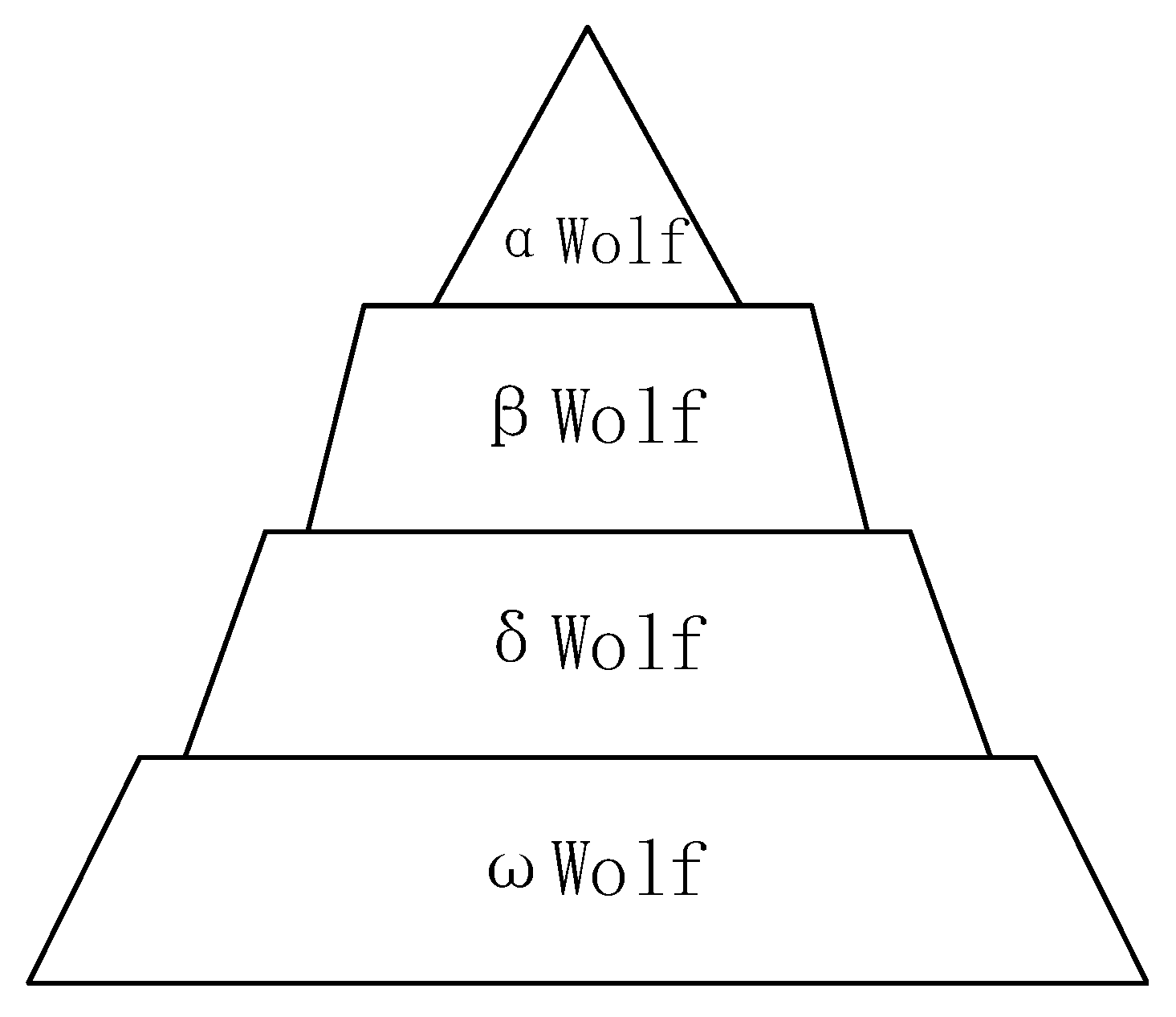
Grey wolves are social animals and have a very strict social hierarchy, as they rely on a clear division of labor and mutual cooperation for survival. According to the habits of the grey wolf, their population can be divided into four levels to conduct mathematical modeling of their hunting technology, as shown in Figure 2.

For the grey wolf group, wolf $\mathsf{\alpha }$ is their leader, responsible for deciding what to hunt, food distribution, sleeping place, wake up time, etc. wolf $\mathsf{\alpha }$ will listen to the advice of other grey wolves, so wolf $\mathsf{\alpha }$ is not necessarily the strongest predator in the pack, but the best wolf in management. In addition, wolf $\mathsf{\alpha }$ is only allowed to mate within the pack. In the hierarchy of GWO algorithm, an $\mathsf{\alpha }$ search agent is considered the best search agent in the population, just like wolf $\mathsf{\alpha }$.

wolf $\mathsf{\beta }$, in the second social rank of the grey wolf, plays the role of subordinate wolf. It carries out the command of wolf $\mathsf{\alpha }$ and transmits the command to other wolves at the same time, and gives the result of execution back to wolf $\mathsf{\alpha }$. When wolf $\mathsf{\alpha }$ dies or becomes sick, wolf $\mathsf{\beta }$ is considered the best replacement for wolf $\mathsf{\alpha }$. Accordingly, the second-best search agent of the GWO algorithm is a $\mathsf{\beta }$ search agent, whose function in the algorithm is similar to that of wolf $\mathsf{\beta }$ in the wolf pack.

wolf $\mathsf{\delta }$ listens to the signals of wolf $\mathsf{\alpha }$ and wolf $\mathsf{\beta }$, but can give orders to wolf $\mathsf{\omega }$. In the pack, wolf $\mathsf{\delta }$ is responsible for guard, hunting, reconnaissance, and other tasks. wolf $\mathsf{\delta }$ must obey the pack’s pecking order and help wolf $\mathsf{\alpha }$ and wolf $\mathsf{\beta }$ when rounding up prey. It also takes care of the young, weak, and sick in the pack. Accordingly, search agent $\mathsf{\delta }$ is considered the third-best search agent in the GWO algorithm.

Except for the $\mathsf{\alpha }$, $\mathsf{\beta }$, and $\mathsf{\delta }$ wolves, the rest of the pack is made up of $\mathsf{\omega }$ wolves. The existence of $\mathsf{\omega }$ wolves can maintain the stability of the hierarchy of the pack, and $\mathsf{\omega }$ wolves also act as babysitters in some cases. In the GWO algorithm, if a search agent is not an $\mathsf{\alpha }$, $\mathsf{\beta }$, and $\mathsf{\delta }$ agent, it is a $\mathsf{\omega }$ search agent. In order to mathematically simulate the group hunting behavior of grey wolves, a $\mathsf{\omega }$ search agent follows the search trajectory of $\mathsf{\alpha }$, $\mathsf{\beta }$, and $\mathsf{\delta }$ search agents, conducts further search around them, and finally finds the global optimal solution [27].

2.2.2. Collective Hunting Behavior of Grey Wolves

Grey wolf predation mainly includes two processes: social hierarchy and group hunting, as shown in Figure 2. The stages of grey wolf hunting can be divided into the following steps:

(1)

Surround the prey

The behavior of rounding up prey is the basis of location updating by $\mathsf{\omega }$ search agents in GWO, and the rounding mechanism can be modeled Equations (6) and (7) as follows:

$$\overrightarrow{D}=\left|\overrightarrow{C}·\overrightarrow{X_p}\left(i\right)-\overrightarrow{X}\left(i\right)\right|$$

(6)

$$\overrightarrow{X}\left(i+1\right)=|\overrightarrow{X_p}\left(i\right)-\overrightarrow{A}·\overrightarrow{D}|$$

(7)

where, $\overrightarrow{X_p}$ represents the position vector of prey, $\overrightarrow{X}$ represents the position vector of a grey wolf, $i$ represents the number of current iterations, and $\overrightarrow{A}$ and $\overrightarrow{C}$ represent the coefficient vector and can be calculated Equations (8) and (9) as follows:

$$\overrightarrow{A}=2\overrightarrow{a}·\overrightarrow{r_1}-\overrightarrow{a}$$

(8)

$$C=2\overrightarrow{r_2}$$

(9)

where, $\overrightarrow{r_1}$ and $\overrightarrow{r_2}$ are arbitrary vectors in the interval [0, 1], and the scaling factor $\overrightarrow{a}$ is time dependent. In the iteration process, the scaling factor $\overrightarrow{a}$ decreases linearly from 2 to 0. The expression Equation (10) as follows:

$$\overrightarrow{a}\left(i\right)=2-\frac{2i}{T_{max}}$$

(10)

where, $T_{max}$ represents the maximum number of iterations.

(2)

Hunt

Grey wolf ranks are not set in stone in wolf packs, and when $\mathsf{\alpha }$, $\mathsf{\beta }$, and $\mathsf{\delta }$ wolves become old, injured, or sick, and become weaker members of the pack, their social ranks are downgraded to $\mathsf{\omega }$ wolves. It is also possible that $\mathsf{\omega }$ wolves could be upgraded to higher-level wolves. Accordingly, in the GWO algorithm, the $\mathsf{\omega }$ search agents follow a random drive mechanism. In this regard, the random driving mechanism of a ω search agents can be mathematically simulated by the following Equation (11):

$$\{\begin{array}{c}\overrightarrow{D_{\alpha }}=\left|\overrightarrow{C_1}·\overrightarrow{X_{\alpha }}-\overrightarrow{X}\right|\\ \overrightarrow{D_{\beta }}=\left|\overrightarrow{C_2}·\overrightarrow{X_{\beta }}-\overrightarrow{X}\right|\\ \overrightarrow{D_{\delta }}=\left|\overrightarrow{C_3}·\overrightarrow{X_{\delta }}-\overrightarrow{X}\right|\end{array}$$

(11)

where $\overrightarrow{X_{\alpha }}$, $\overrightarrow{X_{\beta }},$ and $\overrightarrow{X_{\delta }}$, respectively, represent the first three optimal solutions in the current GWO iteration, and $\overrightarrow{C_1}$, $\overrightarrow{C_2}$, and $\overrightarrow{C_3}$ represent three random coefficient vectors. $\overrightarrow{X}$ represents the current location of the ω search agent.

Equation (11) specifies the estimated span between the current search agent ω and the $\mathsf{\alpha }$, $\mathsf{\beta }$, and $\mathsf{\delta }$ search agents. After estimating the step size of the ω search agent through Equations (8) and (9), the position vector of the final contribution of $\mathsf{\alpha }$, $\mathsf{\beta }$, and $\mathsf{\delta }$ search agents is determined by Equation (12):

$$\{\begin{array}{c}\overrightarrow{X_1}=\overrightarrow{X_{\alpha }}-\overrightarrow{A_1}·\overrightarrow{D_{\alpha }}\\ \overrightarrow{X_2}=\overrightarrow{X_{\beta }}-\overrightarrow{A_2}·\overrightarrow{D_{\beta }}\\ \overrightarrow{X_3}=\overrightarrow{X_{\delta }}-\overrightarrow{A_3}·\overrightarrow{D_{\delta }}\end{array}$$

(12)

where $\overrightarrow{A_1}$, $\overrightarrow{A_2}$, and $\overrightarrow{A_3}$ represent three arbitrary coefficient vectors. Assuming that $\mathsf{\alpha }$, $\mathsf{\beta }$, and $\mathsf{\delta }$ contribute equally to the search agent position vector, the final position of wolf ω is updated by the following Equation (13):

$$\overrightarrow{X}\left(i+1\right)=\frac{\overrightarrow{X_1}+\overrightarrow{X_2}+\overrightarrow{X_3}}{3}$$

(13)

(3)

Attacking prey

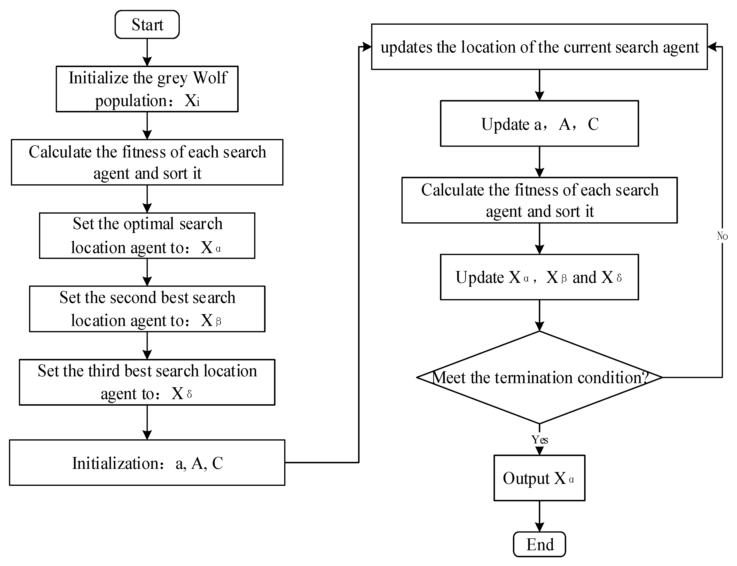
By combining Equation (8), it can be found that it is necessary to divide the range of coefficient vector $\overrightarrow{A}$ into two cases. In order to build a mathematical model approximating the global optimal, the value of $\overrightarrow{a}$ decreases linearly from 2 to 0 in the iterative process. However, the linear reduction in $\overrightarrow{a}$ makes GWO prone to local optimality, also known as stagnation at local optimality. The coefficient vector $\overrightarrow{C}$ is another way to improve the GWO’s exploration capability because it preserves randomness during iteration. The coefficient vector $\overrightarrow{C}$ provides random weights for position updates, which helps the ω search agent to improve the global optimization capability in the iterative process. The randomness of coefficient vector $\overrightarrow{C}$ is included in the whole iteration process, which can alleviate the occurrence of local optimal stagnation. The GWO algorithm is shown in Figure 3.

2.3. Differential Evolutionary Algorithms

Instead of using a separate probability distribution to generate individual fixes, the Differential Evolution (DE) algorithm perturbs the current generation of individuals using a scaled difference vector generated by randomly selected different individuals, in contrast to traditional evolutionary algorithms. A similar computational step to evolutionary algorithms exists, consisting of three operations: variation, crossover, and selection.

Define the population size N; in a D-dimensional search space, $X_{\mathrm{i}}\left(g\right)$ is the i-th individual of the g-th generation, $X_i^L\left(g\right)$ ≤ $X_{\mathrm{i}}\left(g\right)$ ≤ $X_i^U\left(g\right)$, then,

$$X_{\mathrm{i}}\left(g\right)=\left[x_{\mathrm{i}1}\left(g\right),x_{\mathrm{i}2}\left(g\right),\cdots ,x_{\mathrm{in}}\left(g\right)\right];i=1,2,\cdots ,N,g=1,2,\cdots ,t_{\max }$$

(14)

In Equation (14), the $X_i^L\left(g\right)$ is the lower bound of the population individuals, the $X_i^U\left(g\right)$ is the upper bound of the population individuals, and $(t_{\max }$) is the maximum number of iterations. The calculation steps are as follows.

(1)

Randomly generate N initial population individuals throughout the search space

$$x_{\mathrm{ij}}\left(0\right)=x_{ij}^L+rand\left(0, 1\right)\left(x_{ij}^U-x_{ij}^L\right)$$

(15)

In Equation (15), rand (0, 1) is a random number that follows a uniform distribution on [0, 1].

(2)

Variant operations

The following equation generates variant individuals.

$$h_{\mathrm{ij}}\left(g\right)=x_{\mathrm{p}1}+F\left(x_{\mathrm{p}2}-x_{\mathrm{p}3}\right)$$

(16)

In Equation (16), the $x_{\mathrm{p}1},x_{\mathrm{p}2},and x_{\mathrm{p}3}$ are three different parameter vectors chosen randomly from the current population, and $p_1\ne p_2\ne p_3\ne i$, F is the scaling factor between [0, 1].

(3)

Crossover operations

Crossover operations can increase the diversity of populations and are operated as follows.

$$v_{\mathrm{ij}}\left(g+1\right)=\{\begin{array}{c}{h}_{\mathrm{ij}}\left(g\right),rand\left(0, 1\right)\le CR or j=rand\left(1,n\right)\\ x_{\mathrm{ij}}\left(g\right),rand\left(0, 1\right)\le CR or j=rand\left(1,n\right)\end{array}$$

(17)

CR in Equation (17) is the crossover probability between the values [0, 1], and rand (0, 1) is the random number of [0, 1] obeying a uniform distribution. Used to determine that at least one dimensional component comes from the target individual $X_{\mathrm{i}}$

(4)

Select operation

Vector $x_{\mathrm{i}}\left(g\right)$ is compared by the evaluation function on the vectors $v_{\mathrm{i}}\left(g+1\right)$

$$x_{\mathrm{i}}\left(g+1\right)=\{\begin{array}{c}{v}_{\mathrm{i}}\left(g+1\right),f\left[v_{\mathrm{i}}\left(g+1\right)\right]<f\left[x_{\mathrm{i}}\left(g\right)\right]\\ x_{\mathrm{i}}\left(g\right),f\left[v_{\mathrm{i}}\left(g+1\right)\right]\ge f\left[x_{\mathrm{i}}\left(g\right)\right]\end{array}$$

(18)

Thus, this mechanism ensures that at least no child population is inferior to the current individuals, increasing the average performance of the population and creating an optimal solution.

The Differential Evolution algorithm seeks the optimal global solution to the problem to be optimized by finding differences between individuals in the population, then amplifying the different features to form a population of different features and evolving based on a greedy mechanism. The DE algorithm is effective in avoiding becoming trapped in an optimal local solution, but the variational iteration process is slow [28].

2.4. A Hybrid Optimization Model of the Differential Evolution-Grey Wolf Algorithm for SVR Parameter Search

In this paper, an improved nonlinear adjustment strategy is introduced into the time parameter $\overrightarrow{a}$ to improve the exploration and development capability of the DE-GWO. In addition, the location update rule of the GWO algorithm is modified to alleviate the local optimal stagnation phenomenon of the GWO. Finally, an improved GWO algorithm (DE-GWO) based on the idea of hybrid difference vectors is proposed.

2.4.1. Nonlinear Adjustment Strategy of Time Parameter

The time parameter $\overrightarrow{a}$ decreases linearly, ensuring the equal distribution of the exploration phase and development phase in the iterative process. However, the search process of all meta-heuristic algorithms is nonlinear, the search is extremely complex, and linear descent is not consistent with the actual search process. Considering the influence of time parameter $\overrightarrow{a}$ on the GWO algorithm, a new nonlinear time parameter containing a sine function is proposed in this paper. The value of time parameter $\overrightarrow{a}$ varies as follows:

$$\overrightarrow{a}=2-2\left(\frac{i}{T_{max}}\right)+0.3\sin \left(\frac{2i\pi }{T_{max}}\right)$$

(19)

where $i$ indicates the current iteration number, and $T_{max}$ indicates the maximum iteration number. It can be seen from Equation (19) that the value of time parameter $\overrightarrow{a}$ decreases nonlinearly in the iterative process.

2.4.2. Improved Location Update Rules

In the basic GWO algorithm, the assumption that the estimated step sizes of $\mathsf{\alpha }$, $\mathsf{\beta }$, and $\mathsf{\delta }$ search agents contribute equally to the position of search agent ω is not realistic. Too much information about the optimal solutions ($\mathsf{\alpha }$, $\mathsf{\beta }$, and $\mathsf{\delta }$ search agents) of the previous population is shared with the next generation, resulting in a lack of diversity among individuals of the next generation population. The basic GWO algorithm tends to fall into local optima due to over-learning from the optimal search agents obtained so far. Inspired by the idea of Differential Evolution (DE), a differential vector in DE is introduced into the basic GWO algorithm to obtain the improved version (DE-GWO). The formula of difference vector can be written mathematically as follows:

$$\overrightarrow{D}=\overrightarrow{X_a}-\overrightarrow{X_b}$$

(20)

where, $\overrightarrow{X_a}$ and $\overrightarrow{X_b}$ represent any two of the first three optimal solutions generated by the search agent based on $\mathsf{\alpha }$, $\mathsf{\beta }$, and $\mathsf{\delta }$, and $\overrightarrow{D}$ is the generated difference vector. As the population tends to be optimal, the differences between individuals within the population gradually decrease. The fastest rate of convergence is guaranteed by multiplying the difference vector $\overrightarrow{D}$ by a contraction factor F, where $0<$ F $\le$ 1.2. If the difference vector $\overrightarrow{D},$ scaled as required by F, is added to the remainder of the generated optimal solution (except for $\overrightarrow{X_a}$ and $\overrightarrow{X_b}$), a new and improved positional update rule is generated, as follows:

$$\overrightarrow{X}\left(i+1\right)=\overrightarrow{c_1}·\overrightarrow{X_c}+F·\overrightarrow{c_2}·\overrightarrow{D}$$

(21)

where, i represents the current number of iterations, $\overrightarrow{X_c}$ is the remaining one of the first three optimal solutions generated (divided by $\overrightarrow{X_a}$ and $\overrightarrow{X_b}$ outside), F is the scaling factor in the interval (0, 1.2], $\overrightarrow{c_1}$ and $\overrightarrow{c_2}$ are the random vectors in the interval (0, 1), and combined with Equation (20), Equation (21) becomes

$$\overrightarrow{X}\left(i+1\right)=\overrightarrow{c_1}·\overrightarrow{X_c}+F·\overrightarrow{c_2}·\left(\overrightarrow{X_a}-\overrightarrow{X_b}\right)$$

(22)

This is generated due to the basic GWO algorithm. $\overrightarrow{X_{\alpha }}$, $\overrightarrow{X_{\beta }}$, and $\overrightarrow{X_{\delta }}$ are randomly assigned to $\overrightarrow{X_1}$, $\overrightarrow{X_2}$, and $\overrightarrow{X_3}$, and $\overrightarrow{c_1}$ and $\overrightarrow{c_2}$ are random vectors. All of these provide an inevitable impetus for population individuals to roam in the parameter search space. The values of $\overrightarrow{c_1}$ and $\overrightarrow{c_2}$ not only change in the iterative process, but also change among population individuals, so the search performance of the DE-GWO algorithm is strengthened.

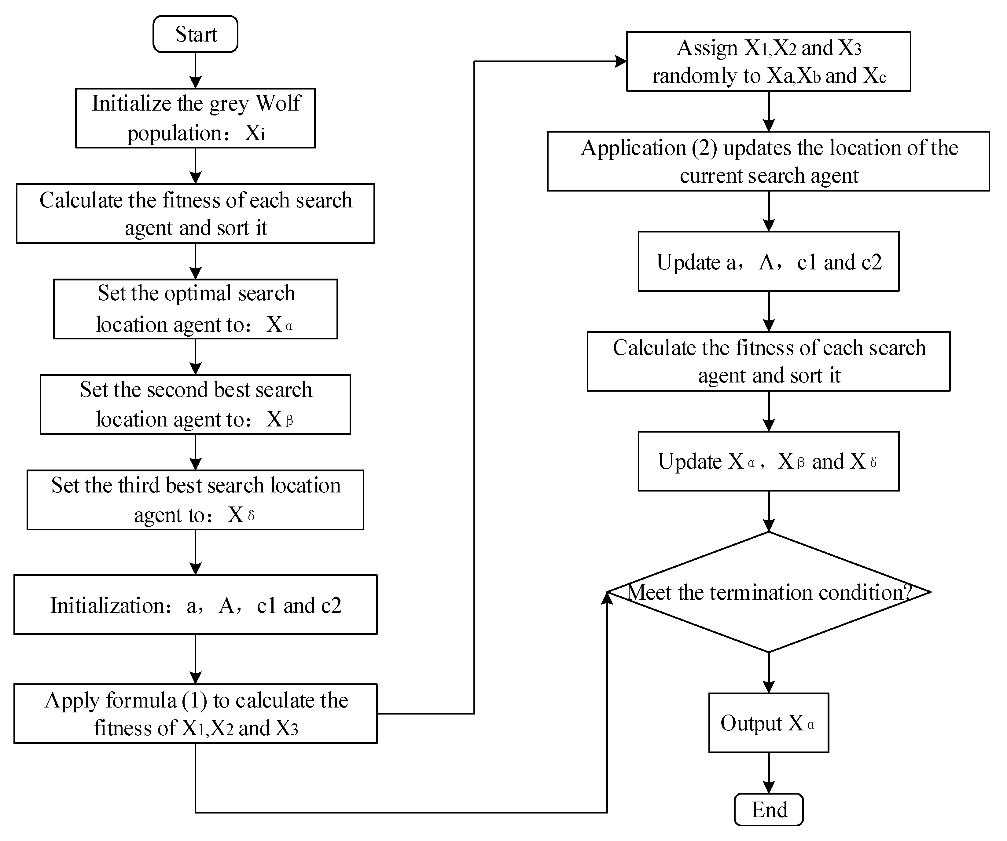
The main difference between the GWO algorithm and DE-GWO algorithm lies in the new position update rules and the new nonlinear adjustment strategy for time parameter $\overrightarrow{a}$. The flow chart of the DE-GWO hybrid optimization algorithm is shown in Figure 4.

3. Experiment

In order to verify the optimization performance of the DE-GWO hybrid optimization algorithm, this paper takes the inversion of a typical water quality parameter experiment as an example. In this paper, we propose using the DE-GWO hybrid optimization algorithm to optimize the support vector regression SVR model’s parameters and the improved SVR model to invert the chlorophyll a and suspended matter concentrations. First, an inversion model of chlorophyll a and suspended matter concentration in Tangdao Bay waters was developed based on the measured hyperspectral data to reduce the influence of atmospheric correction on the inversion accuracy. The model was then applied to the Sentinel II satellite data for remote sensing estimation of chlorophyll a and suspended matter concentrations in the watershed to provide a reference for long-term water quality monitoring and scientific and integrated management of the Tangdao Bay watershed.

3.1. Experimental Data

Tangdao Bay is located in the West Coast New Area of Qingdao, Shandong Province, divided into two shores, the north, and south. Tangdao Bay is located at 119.98 east longitude and 35.88 north latitude. Tangdao Bay has a planned area of 1637.6 hectares, including two categories of offshore and coastal wetlands and artificial wetlands, with a well-preserved ecosystem that is typical and representative of the coastal harbor area in northern China and has high scientific and conservation value. Due to the rapid economic development of the West Coast New Area and the improvement of people’s living standards, there is also a certain impact on the water quality, so it is essential to monitor the area’s water quality using remote sensing.

3.1.1. Measured Spectral Data

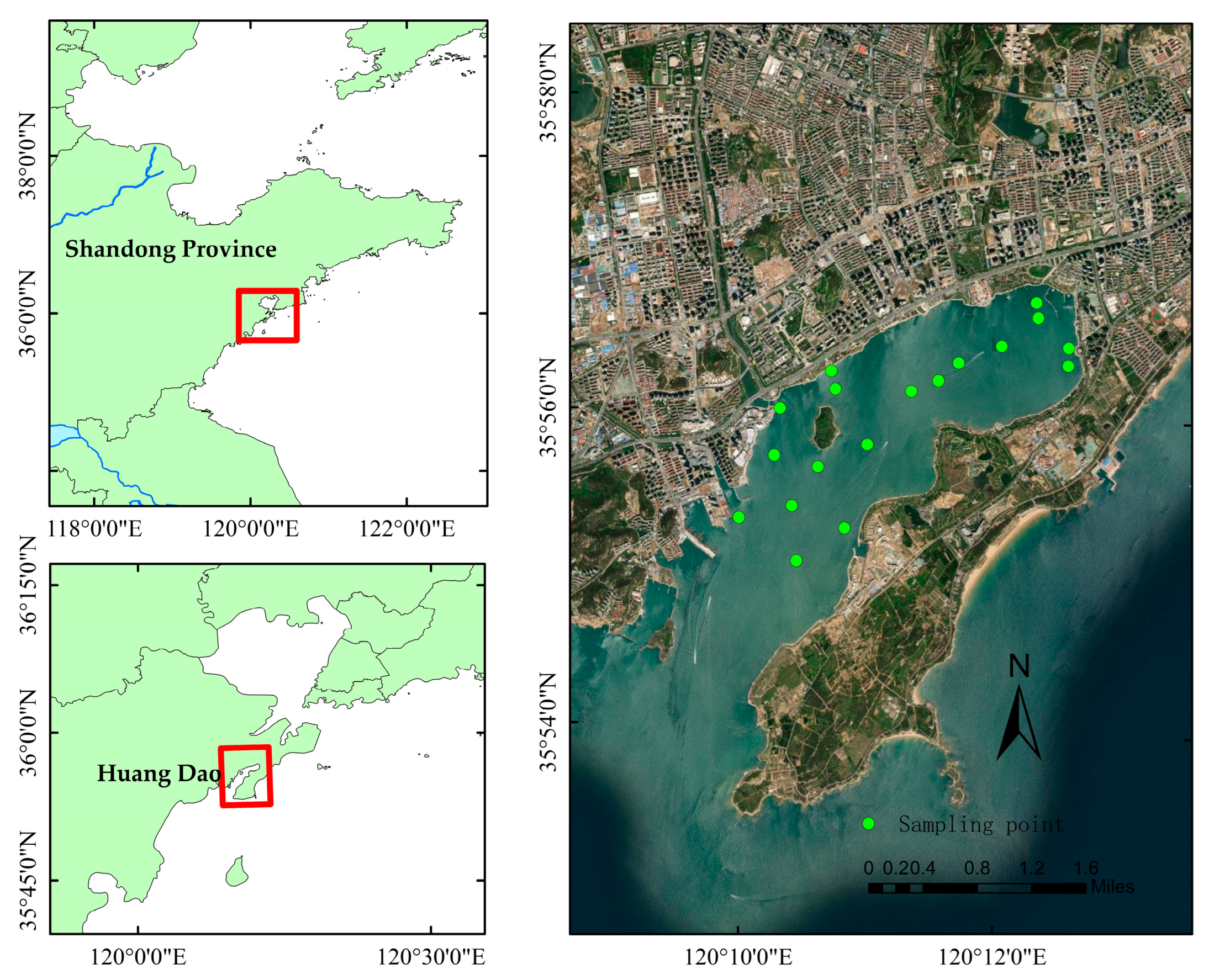
Spectral and water quality parameters were measured at 18 sampling points in Tangdao Bay waters on 8 September 2021. The locations of the sampling sites are shown in Figure 5. The spectral measurements were carried out using the YW-TRIOS-AWRMMS surface moving measurement system (spectral range 320–944 nm, spectral resolution 1 nm), which has a built-in GPS positioning system and can be carried easily for spectral measurements in various situations. During the measurement, the telescopic rod was always oriented at an angle of 135° to the plane of solar incidence, allowing the three sensors to effectively measure the three parameters of solar irradiance, water surface irradiance, and sky irradiance, respectively, and to view the spectral profile in real-time on display. Fifteen sets of spectra were averaged at each sampling point to minimize uncertainty, and the raw spectral data were processed by the method of Mobley (1999) and the spectral data processing procedure to obtain the spectral data information parameters of off-water irradiance and remote reflectance. After the measurement, the abnormal spectral curve was removed.

Water quality parameters at the sampling points were also collected simultaneously on-site. Each sampling point was measured 25 times using the EXO multi-parameter water quality analyzer and averaged to obtain the corresponding chlorophyll a concentration value at the sampling point. Suspended matter concentration values were measured by the weight method [29]. Outliers were removed after the measurement.

3.1.2. Remote Sensing Image Data

Sentinel-2 has two satellites: Sentinel-2A and Sentinel-2B, launched in 2015 and 2017, respectively, with a revisit cycle of 5 days. The Sentinel-2 remote sensing satellite carries a multispectral sensor (MSI). The MSI has 13 bands—4 visible at 10 m, 6 near-infrared bands at 20 m, and 3 bands at 60 m [30]—which cover the electromagnetic spectrum from visible to short-wave infrared wavelengths (0.44–2.2 μm). The orbital strip at ground level is about 290 km.

This experiment downloaded the 1View S2 class L1C product from the European Space Agency’s Copernicus Open Access Centre on 8 September 2021. During the whole experiment cycle of water quality parameters and spectral profile acquisition in Tangdao Bay waters, no natural phenomena such as significant weather changes occurred, so it can be assumed that the image on 8 September can be matched with the acquisition data on that day. For the pre-processing of the Sentinel-2 data, the Sentinel Application Platform version 4.0.2 (http://step.esa.int/main/toolboxes/snap/ (accessed on 15 September 2021)) was used for radiometric calibration and atmospheric correction [31]. The platform has the Sentinel-2 toolbox and the Sen2Cor plug-in version 2.2.1. Sentinel-2 data are radiometrically calibrated and converted to surface reflectance by atmospheric correction using the ATCOR code. After SNAP processing, a standard reflectance product is obtained. Then, the satellite reflectance data for each sample point are extracted using ArcGIS software based on the location of the sample points.

3.2. Typical Water Quality Parameters Concentration Remote Sensing Inversion Model Construction

To carry out remote sensing inversion of chlorophyll a and suspended matter concentrations in Tangdao Bay, first, the spectra were normalized, and correlation analysis was carried out to determine the sensitive band of the inversion model. Then, the inversion model was constructed from the sensitive band and the chlorophyll a and suspended matter concentration values. The inverse model was then constructed from the sensitive bands and the values of chlorophyll a and suspended matter concentrations. The support vector regression SVR model was parameter optimized using the DE-GWO hybrid optimization algorithm. The inversion of the chlorophyll a and suspended matter concentrations was carried out using the optimized SVR model. The model’s accuracy was then verified using satellite reflectance data from Sentinel-2 corresponding to the sampling points. The inversion of typical water quality parameters based on the DE-GWO-SVR model was carried out as follows.

(1)

Correlation analysis between spectral data and concentrations of chlorophyll a and suspended matter.

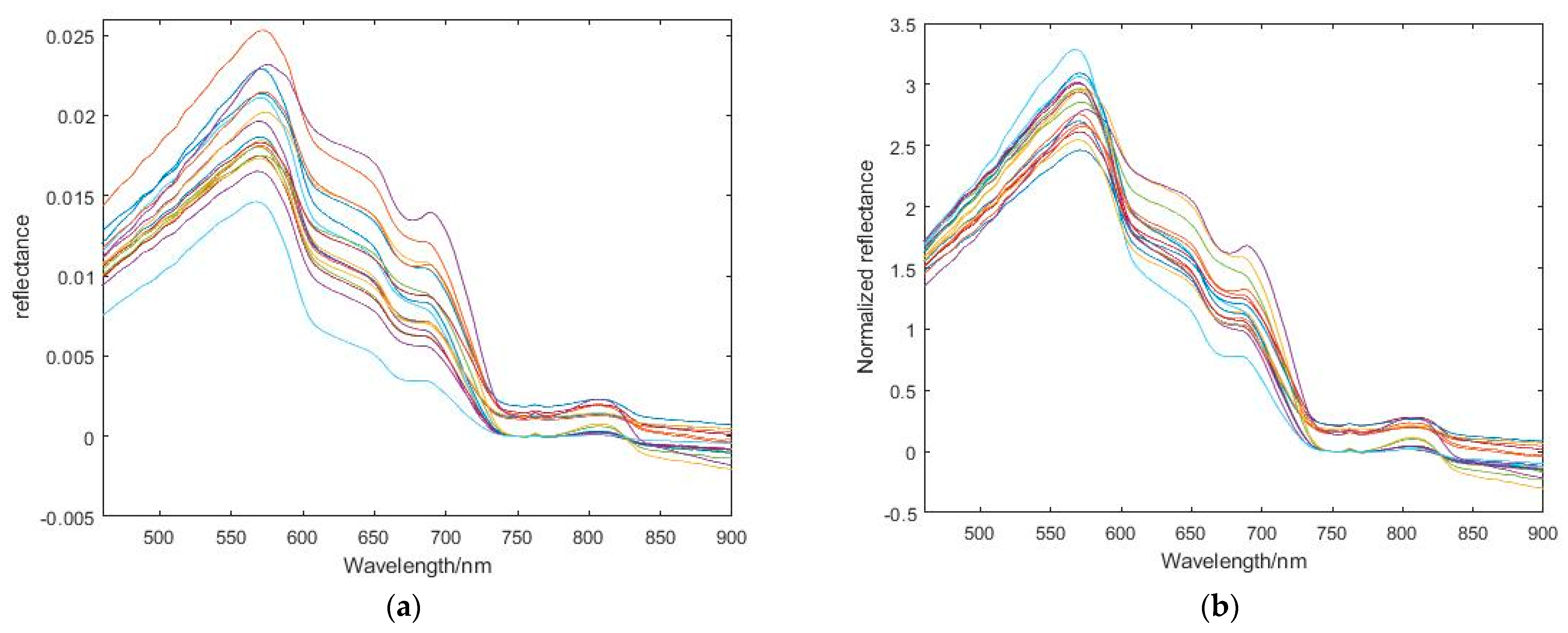
The original spectral curve measured in the field is shown in Figure 6a. After normalization, the result is shown in Figure 6b. The normalized spectral curve has a more pronounced reflectance peak and trough than the original. Pearson correlation analysis is a method to study the strength of the correlation between two or more random variables from the perspective of statistics. When the Pearson correlation analysis was carried out, the input forms included single band, band ratio, band difference, and NDVI-style ratio. It has been shown that the combination of bands can effectively attenuate the effects of other environmental factors, such as water surface smoothness and microwaves [32], thus improving the inversion accuracy of the model.

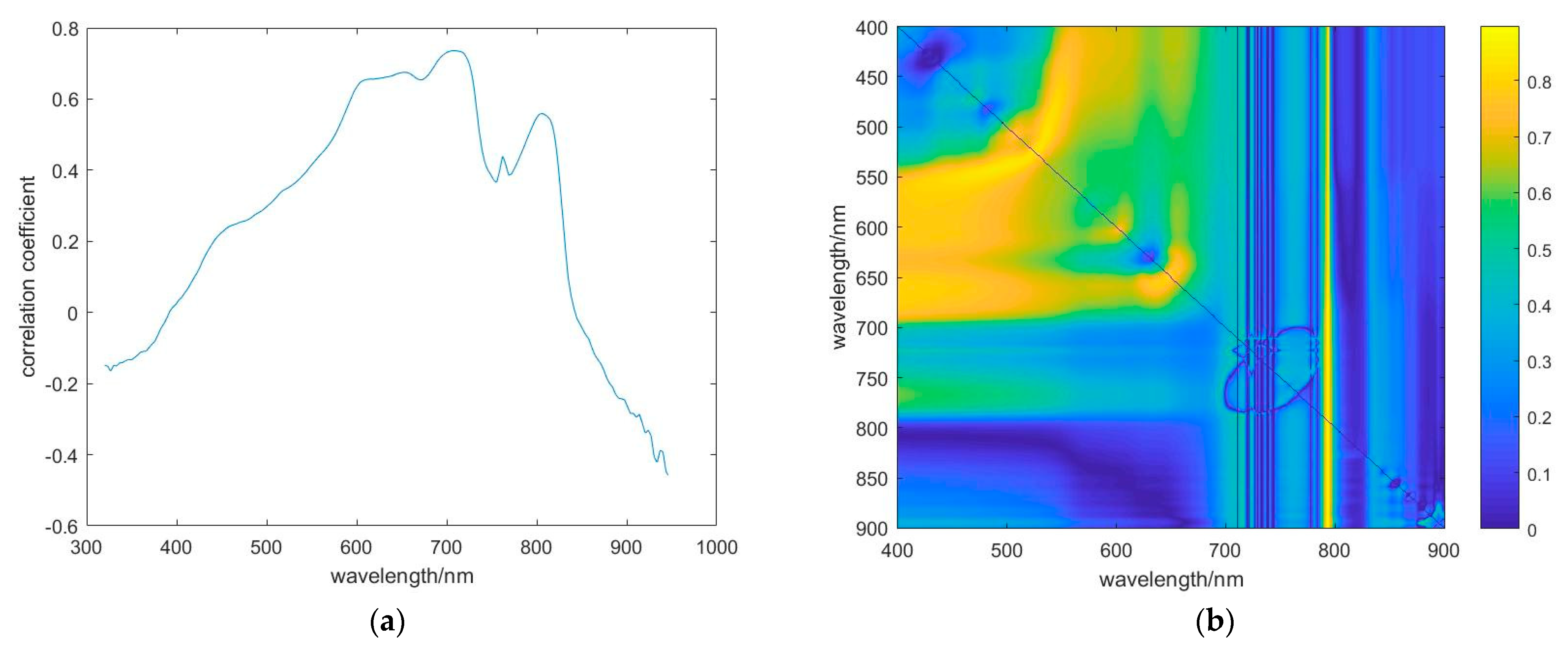
The correlation analysis was conducted between the chlorophyll a and suspended matter concentration values of each sampling point and the single band and band ratio of each set of spectral data, and the results of the correlation analysis were obtained as shown in Figure 7 and Figure 8. The single band and band ratio with the most significant correlation coefficient were selected as the best variables for inversion of chlorophyll a and suspended matter concentration. The results showed that the best band for retrieving chlorophyll a concentration was single band R (711 nm) and band ratio R (569 nm)/R (835 nm), and the correlation coefficients were 0.73 and 0.89, respectively. The best band for inversion of suspended solids concentration was single band R (680 nm) and band ratio R (732 nm)/R (714 nm), and the correlation coefficients were 0.54 and 0.61, respectively.

(2)

Model construction and testing

According to the selected optimal inversion band, this experiment used the measured spectral data of 14 sampling points as training data and 4 as test data to construct the DE-GWO-SVR model, GWO-SVR model, SVR model, and multivariate linear model. Among the DE-GWO-SVR model predictions, the initial parameters of the model were first set as follows: the population size was 60, the maximum number of iterations was 500, and the crossover probability was 0.2. The inversion results of the two water quality parameters are shown in

Table 1. Evaluation parameter results of training set and test set.

Water Quality Parameters	Models	Training Set		Test Set
		R2	MRE/%	R2	MRE/%
Chlorophyll a	Linear regression	0.55	43.2	0.42	48.6
	SVR	0.75	35.1	0.68	39.0
	GWO-SVR	0.81	27.2	0.71	29.1
	DE-GWO-SVR	0.84	25.1	0.76	27.9
SPM	Linear regression	0.46	48.1	0.45	51.6
	SVR	0.74	32.4	0.7	35.5
	GWO-SVR	0.75	30.6	0.69	37.1
	DE-GWO-SVR	0.8	28.1	0.75	32.2

.

The coefficient of determination used to determine the model’s goodness of fit was R². The value of the coefficient is between 0 and 1; the closer to 1, the better the fit of the model. In terms of the goodness of fit R², the coefficient of determination of the DE-GWO-SVR model was 0.84 for the chlorophyll a inversion model and 0.8 for the suspended matter inversion model. However, there were differences between the predicted and measured values of the sampling sites. The determination coefficients were significantly higher than those of the conventional SVR model. The average relative errors of the DE-GWO-SVR models in the test set were much smaller than those of the other models. By comparing the fit and mean relative error results of the DE-GWO-SVR model, GWO-SVR model, SVR model, and multivariate linear model, the improved DE-GWO-SVR model is the best model to achieve effective inversion of typical water quality parameters.

3.3. Typical Water Quality Parameters Concentration Remote Sensing Inversion Model Application

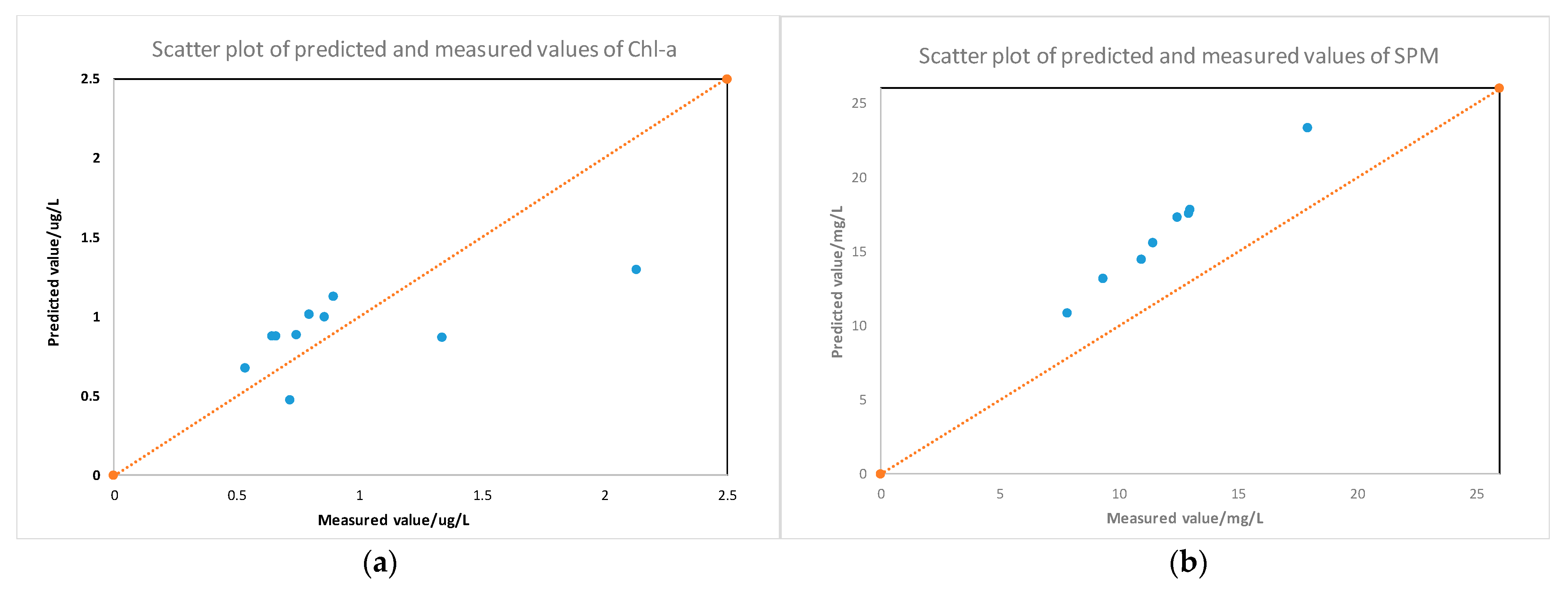
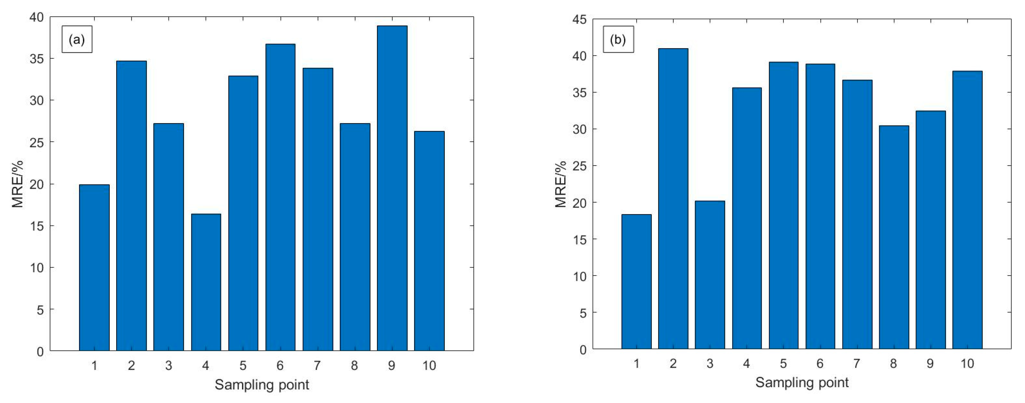
The improved DE-GWO-SVR model was used to convert chlorophyll a and suspended matter concentration on Sentinel-2 satellite data. To further validate the model’s accuracy on Sentinel-2 satellite images, 10 sampling points were selected for validation at the same time and location as the Sentinel-2 satellite image acquisition, and the correlation between the inversion values of the sampling points and the measured values was analyzed. The scatter plots of the inversion values of the sampled points and the measured values were obtained by statistical regression, as shown in Figure 9. The relative error results of each issue are shown in Figure 10.

The line in Figure 6 is the deviation line of the data distribution; the closer the inverse value is to the deviation line, the closer the inverse value is to the measured value, and the farther the deviation line is, the larger the difference. The coefficient of determination for fitting the inverse chlorophyll a concentration to the estimated value was 0.74, with 10 points distributed near the deviation line; the minimum relative error was 19.9%, and the average relative error of the 10 points was 29.4%. The average relative error of the 10 points was 33.0%. The inversion results of the two water quality parameters were similar to the accuracy of the inversion of water quality parameters from other satellite remote sensing images [33,34,35,36]. In summary, although the predicted values of some sampling points were somewhat different from the measured values, it can still be seen that the inversion results of the DE-GWO-SVR model showed good correlation and consistency with the measured values, indicating that the model can achieve effective inversion of the concentrations of typical water quality parameters.

As seen in Figure 7, the inversion results for some of the sampling points based on Sentinel-2 satellite remote sensing data differ slightly from the measured concentration values, presumably because of the difference in data quality between the two. The TRIOS sensor used to collect the measured spectra differs from the Sentinel-2 satellite sensor, and the sensor has a different set of parameters, such as signal-to-noise ratio. The results suggest that the sampling points should be located as far away from the shore as possible to minimize the influence of non-aqueous pixels on the coast of Tangdao Bay and that the slight swaying of the ship during the acquisition of the spectra leads to significant differences between some of the inversion results and the measured values.

4. Discussion

In order to address the impact of water environmental problems on ecosystems and achieve high-precision remote sensing inversion of typical water quality parameters such as chlorophyll a and suspended sediment concentration, especially in Class II water bodies, this study utilized water quality parameter data and spectral data measured in the Tangdao Bay waters on 8 September 2021, and constructed a DE-GWO-SVR model to predict the chlorophyll a and suspended sediment concentration in Tangdao Bay. The evaluation results show that the DE-GWO-SVR hybrid optimization model has good feasibility and predictability in the region. Compared with the MRE of the SVR model, the prediction errors of the DE-GWO-SVR model were reduced by 11.1% (chlorophyll a concentration) and 3.3% (suspended matter concentration). This analysis demonstrates that the DE-GWO-SVR model has better prediction accuracy for both chlorophyll a and suspended matter concentrations in the region than the SVR model. Other research results indicate that the optimized SVR algorithm significantly improves the prediction accuracy in predicting the process variables of marine protease fermentation [37], forecasting meteorological droughts [38], and predicting the geo-mechanical properties of rocks [39], compared to the original SVR model.

To address the problem of premature convergence and becoming stuck in local optima in the GWO algorithm, this study introduces a sine function into the time parameter $\overrightarrow{a}$ based on the traditional Grey Wolf Optimizer algorithm, which makes it nonlinearly decrease during the iteration process to improve the search ability of the GWO algorithm. Additionally, the position updating rule of the GWO algorithm is improved to alleviate the problem of local optima stagnation. The research results show that the MRE (Mean Relative Error) of the DE-GWO-SVR model, which has been improved, decreased by 1.2% (chlorophyll a concentration) and 4.9% (suspended solids concentration) compared to the GWO-SVR model. In the prediction of suspended solids concentration, the prediction accuracy of the GWO-SVR model decreased compared to the original SVR model, indicating that the GWO algorithm may have been trapped in a local optimum during the optimization process of SVR, resulting in a decrease in the model’s prediction ability. Overall, the improved DE-GWO-SVR model can effectively solve the problem of the GWO algorithm easily falling into local optima and has better prediction accuracy in the inversion of typical water quality parameters. This is consistent with the research results of Sun [40] in the prediction of steel thickness, indicating that the prediction performance of the HGWO-SVR model improved by the coefficient vector is better than that of the GWO-SVR and SVR models.

To verify the generalization ability of the DE-GWO-SVR algorithm on satellite remote sensing images, this study used synchronous Sentinel-2 satellite remote sensing reflectance data and selected 10 sampling points as detection points. The DE-GWO-SVR model was used to invert the water quality parameter concentration. From Figure 9 and Figure 10, it can be seen that the model still has good inversion accuracy. Currently, the accuracy of chlorophyll a concentration inversion requires the error to be no more than 50% for type II water bodies [41]. The inversion results of Sentinel-2 data demonstrate the effectiveness of remote sensing inversion for chlorophyll a and suspended solids concentrations.

When modeling using measured spectral data in this study, we obtain the sensitive factors of chlorophyll a and suspended matter concentration through Pearson correlation analysis; whether these sensitive factors can be used as sensitive factors for inverting water quality parameters in other water bodies still needs to be further studied. Meanwhile, the inversion results of Sentinel-2 satellite remote sensing data show a slightly larger discrepancy with the measured values, which is suspected to be due to uneven data quality. Since the TRIOS spectral measurement instrument and Sentinel-2 satellite are two completely different sensors, the parameters such as signal-to-noise ratio of the sensors are not consistent, so the data quality obtained by the two instruments is not consistent. The study shows that chlorophyll and suspended matter have a very sensitive response to the optical characteristics of water bodies. In order to reduce the impact of non-aquatic pixels near the shore, sampling points are selected as far away from the shore as possible. When using the DE-GWO algorithm to optimize the parameter values of the SVR model, the population is usually initialized in a random manner, which makes it difficult to ensure the diversity of the population and results in a slow convergence speed of the algorithm. Due to the limited number of samples, the applicability of this model in other water bodies needs further investigation.

5. Conclusions

Based on the Grey Wolf Optimizer algorithm, this paper develops the DE-GWO algorithm to address its shortcomings, such as local optima stagnation, low solution accuracy, and slow convergence rate. We use DE-GWO to optimize the parameters of the SVR model and establish a water quality parameter inversion model based on the optimized SVR parameters. Finally, the model is validated through experiments.

The main conclusions of this paper are as follows:

(1)

To address the shortcomings of the Grey Wolf Optimizer algorithm, such as local optima stagnation, low solution accuracy, and slow convergence rate, we introduce a nonlinear adjustment strategy for the time parameter $\overrightarrow{a}$ and improve the position update rule. Based on these improvements, we design a hybrid optimization algorithm called the DE-GWO algorithm.

(2)

We introduce the DE-GWO algorithm to optimize the parameters of the SVR model and compare and analyze it with various prediction methods such as multiple linear regression, SVR, and GWO-SVR methods. The results demonstrate that the inversion accuracy of the DE-GWO algorithm is significantly better than that of other models, and the prediction results are relatively stable. When the model is applied to the satellite remote sensing data of Sentinel-2, it still demonstrates good predictive performance. This indicates that the water quality parameter inversion method based on measured spectra and satellite images has good application prospects and promotion value.

The DE-GWO-SVR model based on measured spectra showed good performance in the Tangdao Bay water area, but its application performance in other complex water environments still needs further study. When using the GWO and DE-GWO to optimize the SVR algorithm, the random initialization method is usually adopted to initialize the population, and the diversity of the population is difficult to guarantee. In subsequent studies, some algorithms can be used to initialize the population to further improve the optimization performance of the algorithm. Therefore, the next step is to collect data on a wide range of water bodies and other water quality parameters to conduct a more comprehensive evaluation of the DE-GWO-SVR model method. Recommended and forthcoming future work includes the following:

(1)

In order to improve the predictive accuracy of our model, we will continue to conduct water experiments to expand our sample library.

(2)

We may use chaotic mapping to initialize the population, increase population diversity, and improve the convergence speed and optimization performance of the DE-GWO algorithm.

(3)

We will use other satellite remote sensing data (such as MODIS, GOCI, etc.) to conduct experiments in multiple water bodies to improve the applicability of the model.

References

1. Ding, H.; Wang, D. Eutrophication degree evaluation method based on cloud model. Acta Sci. Circumstantiae 2013, 33, 251–257. [Google Scholar]
2. Gordon, H.R.; André, Y.M. Remote Assessment of Ocean Color for Interpretation of Satellite Visible Imagery; Springer: Berlin/Heidelberg, Germany, 1983. [Google Scholar]
3. Cheng, C.M.; Li, Y.; Ding, Y.; Tu, Q.G.; Peng, Q. Remote sensing estimation of chlorophyll a and total suspended solids concentration in Qiantang River based on GF-1/WFV. J. Yangtze River Sci. Res. Inst. 2019, 36, 21–28. [Google Scholar]
4. Cole, B.E.; Cloern, J.E. An empirical model for estimating phytoplankton productivity in estuaries. Mar. Ecol. Prog. 1987, 36, 299–305. [Google Scholar] [CrossRef]
5. Dennison, W.C.; Orth, R.J.; Moore, K.A.; Stevenson, J.C.; Carter, V.; Kollar, S.; Bergstrom, P.W.; Batiuk, R.A. Assessing Water Quality with Submersed Aquatic Vegetation. Bioscience 1993, 43, 86–94. [Google Scholar] [CrossRef]
6. Miller, R.L.; McKee, B.A. Using MODIS Terra 250 m imagery to map concentrations of total suspended matter in coastal waters. Remote Sens. Environ. 2002, 93, 259–266. [Google Scholar] [CrossRef]
7. Chen, Z.; Hu, C.; Muller-Karger, F. Monitoring turbidity in Tampa Bay using MODIS/Aqua 250-m imagery. Remote Sens. Environ. 2007, 109, 207–220. [Google Scholar] [CrossRef]
8. Zhang, Y.; Zhang, B.; Ma, R.; Feng, S.; Le, C. Optically active substances and their contributions to the underwater light climate in Lake Taihu, a large shallow lake in China. Fundam. Appl. Limnol. 2012, 170, 11. [Google Scholar] [CrossRef]
9. Duan, H.; Ma, R.; Zhang, Y.; Zhang, B. Remote-sensing assessment of regional inland lake water clarity in northeast China. Limnology 2009, 10, 135. [Google Scholar] [CrossRef]
10. Dihkan, M.; Karsli, F.; Guneroglu, A. Mapping total suspended matter concentrations in the black sea using landsat TM multispectral satellite imagery. Fresen Environ. Bull. 2011, 20, 262–269. [Google Scholar]
11. Liu, S.Y.; Tai, H.J. A hybrid approach of support vector regression with genetic algorithm optimization for aquaculture water quality. Math. Comput. Model. 2013, 58, 458–465. [Google Scholar] [CrossRef]
12. Xue, T.L.; Zhao, D.F.; Han, F. Research on water quality prediction model of SVR based on GA optimization. Environ. Eng. 2020, 38, 123–127. [Google Scholar]
13. Cui, H.; Yu, X.L.; Pang, J.W.; Yang, S.H.; Ren, N.Q.; Ding, J. A soft measurement model for influent BOD using BP-ANN and improved SVR. J. Harbin Inst. Technol. 2022, 54, 59–66. [Google Scholar]
14. Mahmoudi, N.; Orouji, H. Integration of Shuffled Frog Leaping Algorithm and Support Vector Regression for Prediction of Water Quality Parameters. Water Resour. Manag. 2016, 30, 2195–2211. [Google Scholar] [CrossRef]
15. Sheng, H.; Chi, H.X.; Xu, M.M.; Liu, S.W.; Wan, J.H.; Wang, J.J. Improved SVR for hyperspectral remote sensing inversion of COD in inland water bodies. Spectrosc. Spect. Anal. 2021, 41, 3565–3571. [Google Scholar]
16. He, Z.X.; Bao, X.Y. Comprehensive evaluation of groundwater quality based on improved PSO optimized SVR. J. Occup. Health 2021, 41, 26–32. [Google Scholar]
17. He, Z.L.; Guo, Z.J.; Yang, J.G. Study on the prediction of residual chlorine in water supply system based on PSO-SVR model. J. Yangtze River Sci. Res. Inst. 2015, 32, 6–10. [Google Scholar]
18. He, T.D.; Li, M.W.; Huang, H. A water quality evaluation method for SVR with PSO preferred parameters. Comput. Eng. Appl. 2010, 46, 11–14. [Google Scholar]
19. Guo, L.J.; Li, B.L. Study on soft measurement of total nitrogen in effluent based on GNFA-SVR. Ind. Water Treat. 2022, 42, 111–117. [Google Scholar]
20. Zhang, Y.J.; Kang, C.L.; Liu, Y.Q.; Fu, X.G.; Zhang, J.X.; Wang, M.X.; Yang, L.Z. Rapid detection of total nitrogen and total phosphorus in water based on surface-enhanced Raman spectroscopy and GWO-SVR algorithm. Spectrosc. Spect. Anal. 2021, 41, 3147–3152. [Google Scholar]
21. Zheng, W.; Li, Z.; Jia, H.; Gao, C. Research on steelmaking end point prediction model based on improved whale optimization algorithm and least square support vector machine. Camb. J. Econ. 2019, 47, 700–706. [Google Scholar]
22. Ehteram, M.; Sharafati, A.; Asadollah, S.B.H.S. Estimating the transient storage parameters for pollution modeling in small streams: A comparison of newly developed hybrid optimization algorithms. Environ. Monit. Assess. 2021, 193, 475. [Google Scholar] [CrossRef]
23. Mirjalili, S.; Mirjalili, S.M.; Lewis, A. Grey Wolf Optimizer. Adv. Eng. Softw. 2014, 69, 46–61. [Google Scholar] [CrossRef]
24. Kang, C.L. Research on the Detection of Pollutants in Water Based on SERS Technology and GWO-SVR Algorithm. Ph.D. Thesis, Yanshan University, Hebei, China, 2021. [Google Scholar]
25. Zhou, P.J. Construction and Application of Water Quality Prediction Model Based on PLS-GWO-SVR. Ph.D. Thesis, Yanshan University, Hebei, China, 2020. [Google Scholar]
26. Ge, T.; He, K.; Ke, Q.; Sun, J. Optimized product quantization for approximate nearest neighbor search. In Proceedings of the 2013 IEEE Conference on Computer Vision and Pattern Recognition, Portland, OR, USA, 23–28 June 2013. [Google Scholar]
27. Tan, F.M.; Zhao, J.J.; Wang, Q. A study on a gray wolf optimization algorithm with an improved nonlinear convergence method. Microelectron. Comput. 2019, 36, 89–95. [Google Scholar]
28. Yang, X.S.; Deb, S. Cuckoo search via levy flights. In Proceedings of the 2009 World Congress on Nature Biologically Inspired Computing NaBIC, Coimbatore, India, 9–11 December 2009; pp. 210–214. [Google Scholar]
29. Zhou, H.L.; Zhu, J.H.; Han, B.; Chen, J. Research on the key technology for measuring suspended matter concentration by weight method. Ocean. Technol. 2004, 23, 6. [Google Scholar]
30. Aguilera, M.A.Z. Classification of land-cover through machine learning algorithms for fusion of sentinel-2a and planetscope imagery. In Proceedings of the 2020 IEEE Latin American GRSS & ISPRS Remote Sensing Conference (LAGIRS), Santiago, Chile, 22–26 March 2020. [Google Scholar]
31. Wang, J.; Ding, J.; Yu, D.; Ma, X.; Zhang, Z.; Ge, X.; Teng, D.; Li, X.; Liang, J.; Lizaga, I.; et al. Capability of Sentinel-2 MSI data for monitoring and mapping of soil salinity in dry and wet seasons in the Ebinur Lake region, Xinjiang, China. Geoderma 2019, 353, 172–187. [Google Scholar] [CrossRef]
32. Parida, B.R.; Kumari, A. Mapping and modeling mangrove biophysical and biochemical parameters using Sentinel-2A satellite data in Bhitarkanika National Park, Odisha. Model Earth Syst. Eny. 2021, 7, 2463–2474. [Google Scholar] [CrossRef]
33. El-Rawy, M.; Fathi, H.; Abdalla, F. Integration of remote sensing data and in situ measurements to monitor the water quality of the Ismailia Canal, Nile Delta, Egypt. Environ. Geochem. Health 2019, 42, 2101–2120. [Google Scholar] [CrossRef]
34. Gao, C.; Xu, J.; Gao, D.; Wang, L.L.; Wang, Y.Q. Inversion of total suspended solids concentration in Poyang Lake based on GF-1 and measured spectral data during the abundant water period. Remote Sens. Land Resour. 2019, 31, 101–109. [Google Scholar]
35. Liu, X.; Lee, Z.; Zhang, Y.; Lin, J.; Shi, K.; Zhou, Y.; Qin, B.; Sun, Z. Remote Sensing of Secchi Depth in Highly Turbid Lake Waters and Its Application with MERIS Data. Remote Sens. 2019, 11, 2226. [Google Scholar] [CrossRef]
36. Lu, S.; Deng, R.; Liang, Y.; Xiong, L.; Ai, X.; Qin, Y. Remote Sensing Retrieval of Total Phosphorus in the Pearl River Channels Based on the GF-1 Remote Sensing Data. Remote Sens. 2020, 12, 1420. [Google Scholar] [CrossRef]
37. Li, Z.; Rehman, K.U.; Wenhui, L.; Atique, F. Soft Sensor Modeling Method Based on SPA-GWO-SVR for Marine Protease Fermentation Process. J. Control. Sci. Eng. 2021, 2021, 6653503. [Google Scholar] [CrossRef]
38. Malik, A.; Tikhamarine, Y.; Souag-Gamane, D. Support vector regression integrated with novel meta-heuristic algorithms for meteorological drought prediction. Meteorol. Atmos. Phys. 2021, 133, 891–909. [Google Scholar] [CrossRef]
39. Xu, C.H.; Nait Amar, M.; Ghriga, M.A.; Ouaer, H.; Zhang, X.; Hasanipanah, M. Evolving support vector regression using Grey Wolf optimization; forecasting the geomechanical properties of rock. Eng. Comput. 2020, 38, 1819–1833. [Google Scholar] [CrossRef]
40. Sun, L.; Li, J.; Xiao, X.; Zhang, L.; Li, J. Improved Differential Gray Wolf Algorithm Optimized Support Vector Regression Strip Thickness Prediction Method. Eng. Lett. 2021, 29, 1462–1469. [Google Scholar]
41. Zhang, X.Y.; Wan, J.H.; Liu, S.W.; Song, D.M. Construction of chlorophyll a extraction index and concentration inversion of high suspended matter concentration in the Yellow River Estuary based on GOCI data. Ocean. Technol. 2022, 41, 19–20. [Google Scholar]
Figure 1. SVR model diagram.
Remotesensing 15 02104 g001
Figure 2. The division of grey wolf social hierarchy.
Remotesensing 15 02104 g002
Figure 3. GWO algorithm flow chart.
Remotesensing 15 02104 g003
Figure 4. DE-GWO algorithm flow chart.
Remotesensing 15 02104 g004
Figure 5. The maps of Tangdao Bay.
Remotesensing 15 02104 g005
Figure 6. Original and normalised spectral curves. (a) is the original spectral curve, (b) is the normalised spectral curve.
Remotesensing 15 02104 g006
Figure 7. Pearson correlation analysis of single band, band ratio, and chlorophyll a concentration: (a) single band; (b) band ratio.
Remotesensing 15 02104 g007
Figure 8. Pearson correlation analysis of single band, band ratio, and SPM concentration: (a) single band; (b) band ratio.
Remotesensing 15 02104 g008
Figure 9. Image sampling point inversion value and measured value scatter plot: (a) Chlorophyll a; (b) SPM.
Remotesensing 15 02104 g009
Figure 10. The relative error diagram of the inversion value and the measured value of the sampling point: (a) Chlorophyll a; (b) SPM.
Remotesensing 15 02104 g010