1. Introduction
David Glacier is the largest outlet glacier in Northern Victoria Land, collecting a catchment area of approximately 4% of East Antarctica [
1]. Its basin extends to Dome C and Talos Dome and produces a floating ice tongue of about 140 km long from the grounding zone and about 20 km wide, with 90 km of longitudinal extent not extending into the Ross Sea. As most of David Glacier basin is below the sea level, it is a marine-based glacier, with the grounding line about 2000 m below the sea level [
2,
3]. Basal melting at the grounding line position is estimated at 29 ± 6 m ice/yr [
1,
2]. Further downstream, basal melting decreases by a factor of two. Due to its size, the David-Drygalski ice system affects local ocean circulation and the persistence of the polynya within Terra Nova Bay. At the point where the David Glacier crosses the Transantarctic Mountains, there is a steep change in slope of the basal topography of the glacier, which generates an icefall, the so-called David Cauldron, not far from the area in which it is assumed the grounding line occurs [
4]. The David-Drygalski has been studied for a long time, since the early 1990s [
2,
5,
6,
7,
8,
9,
10,
11,
12,
13,
14,
15]. Current studies on the coupling between glaciers and bedrock identify the prevailing processes by which ice flows onto the bedrock before arriving at the grounding zone; these are regeneration and plastic flow. Danesi et al. [
16] observed an intense seismicity, clustered in time and space, at the base of the David Cauldron, which abruptly stopped after 2004; between 2003 and 2016 two significant seismic clusters were recorded upstream of the icefall, which highlighted the influence of basal lubrication conditions on seismic events. Finally, they observed at the end of 2003 a strong correlation between the sea tide and the icequake time series with a period of 14 days. The latter was analyzed in Vittuari et al. [
17], and it was found to be the period of passage of the moon at the equator that forces the variation in the amplitude of the sea tide in the area and influences the horizontal velocity of the ice flow. Moon et al. [
14], through a 3-year observation derived by synthetic aperture radar (SAR) offset tracking observations, show that the velocity observed astride the David Cauldron tends to increase during the Antarctic summer. The geodetic monitoring of the floating and grounded parts of the David Glacier can underline how much the GNSS data collected and well documented in the past can provide useful information today for further studies and evaluations, thanks to the advancement of analysis techniques.
In this study, we employed recent GNSS post-processing techniques using the kinematic precise point positioning (KPPP) undifferentiated approach. The latter was applied on two datasets, each lasting 24 days, collected in 2006, close to the grounding line and downstream of it. In this paper, two lines are reported: the first defined within the Polar Year Project ASAID [
4], and the second within the Project MEaSUREs Antarctic Grounding Line from Differential Satellite Radar Interferometry, Version 2 [
18,
19,
20].
One of the strengths of the method is that of being able to compare, in a very detailed way, daily signals coming from receivers placed in very different positions on the David Glacier, thus highlighting the influence of the tide on its horizontal and vertical movements. The spatial analysis was then extended using synthetic aperture radar (SAR), through the processing of three pairs of Cosmo-SkyMED Stripmap scenes. This makes it possible to evaluate the variations in the daily velocity of the ice flow over a period of fifteen days, considering the cycle induced in the ocean tide by the passage of the moon at the equator.
The fact that the David Glacier is a marine-based glacier means that it is particularly sensitive to changes in ocean conditions, such as warming ocean temperatures or the influx of warm water from currents. Understanding the behavior and response of marine-based glaciers like the David Glacier is an important area of research in understanding the impacts of climate change on the Antarctic Ice Sheet.
2. Ice Flow Derived by Geodetic GNSS Observations
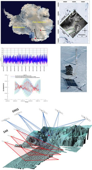
The David Glacier has two major feed streams: the main southern flow from Dome Circe and the slower-moving northern flow from Talos Dome, which merge. In this paper, the control points are located only within the southern flow and no information can be extracted from this analysis about the northern flow. To understand some characteristics of the dynamics of the southern ice flow and the effect of the ocean tide on the movements of the floating and grounded parts of David Glacier, two dual-frequency GNSS geodetic receivers were installed on its surface at the end of 2006. These stations have become part of an observation network of seismic stations already operating in the study area [
21].
To accomplish the above, the first station was installed at ICF1, close to the area where the flotation zone of David Glacier is assumed to start, and the second station was at DRY1, approximately 40 km downstream of ICF1 and 100 km from the edge of the Ross Sea (
Figure 1). Unfortunately, when the experiment was set up, the GNSS master station, installed on a rocky outcrop near the ice tongue, for some unidentified reason, stopped acquiring after a few days of operation. To overcome the problem, some satisfactory results have been achieved in post-processing, adopting the double difference technique, using data from a permanent GNSS station (TNB1), about 100 km away from the study area, at the Mario Zucchelli station (MZS) [
21].
Nowadays, the undifferenced GNSS post-processing analysis technique (Precise Point Positioning), together with the recent improvements available for the kinematic reconstruction of the position of a single GNSS instrument, with a sampling rate of even less than one minute, allow a detailed reanalysis of such data, highlighting signals that were not detectable with the analysis techniques used at the time of the experiment.
Reference [
17] includes comparisons between a double-difference approach using the Track Gamit-Globk software and the undifferentiated PPP approach using the Bernese GNSS software, Version 5.2. Given the distance of about 100 km from the reference station located on granite outcrops at Mario Zucchelli Station, the second solution is less noisy and does not have outliers that can reach and exceed one meter, which are present in the first solution. Some specifics on GNSS monumentation are provided here, as it is an important aspect of any geodetic installation, especially one built on a moving ice body with temperatures and winds varying suddenly and rapidly. The procedure that follows was repeated for each installation point. Starting from previous experience with GNSS measurements in similar conditions, a 3 m long aluminum pole of about 13 cm diameter was driven about one meter into the ice at the chosen position (
Figure 2). A hollow aluminum pole with a diameter sufficient to counteract vertical oscillations has two great advantages compared with other types of materials. Since the thickness of the metal is only a few mm, it is very light and tends to cool down and anchor itself very efficiently to the ice in which it is fixed, as it anchors very strongly inside and outside the circular section. Moreover, the variation in the length of pole due to the thermal expansion (26.3 × 10
−6 m per meter per Celsius degree) can be considered negligible. Then, a self-centering device was inserted at the top of the pole to fix the GNSS antenna.
Each instrument system was powered by two batteries recharged by solar panels. Since the installation points were reached by helicopter, the size and weight of the GNSS station facilities were designed to be easily transported considering the space available inside the Squirrel helicopter and in the basket placed above the skid.
Two GNSS units were used for the survey, each composed of a Trimble 5700 geodetic receiver equipped with a Trimble Zephyr antenna; the sampling rate of the raw acquisitions was fixed at 15 s. The GNSS receiver, together with the batteries and the electronic control unit, were placed inside insulated boxes to protect the instrumentation from temperature and ice. The collected GNSS data was then processed using the Precise Point Positioning (PPP) approach, implemented in the Bernese V5.2 software [
22], to obtain a kinematic averaged solution every 5 min.
The PPP technique allows the position of a single receiver to be determined with centimeter-level accuracy [
23], using undifferenced dual-frequency code and phase observations, whether the phase ambiguity resolution was successful. CODE/IGS products such as satellite orbits, Earth orientation parameters (EOP), satellite clock corrections, and absolute antenna phase center variation (PCV) models were used in the calculation, together with IGS products for the atmosphere modeling. Solid Earth tides, Earth rotation, and ocean tidal loading were applied according to IERS 2010 Conventions [
24]. PPP processing implies ionosphere-free combinations of multifrequency pseudorange and carrier-phase observations to estimate the unknown parameters by fixing satellite coordinates and satellite clock parameters. Receiver coordinates, the troposphere, carrier phase ambiguities, and the receivers’ clock parameters were estimated in a consistent way with respect to the global reference system defined by the satellite ephemerides and the ancillary products.
The PPP processing was part of an automated pipeline that starting from the daily observations to produce the estimate of the coordinates based on the user-defined kinematic sampling interval. To achieve the desired result, some modifications were made to the software, in particular to the client Perl scripts, in order to manage high-frequency outputs. The results were processed through Perl scripts and Fortran95 routines to obtain input files for the Matlab Tsview software [
25] used for interactive time series analysis.
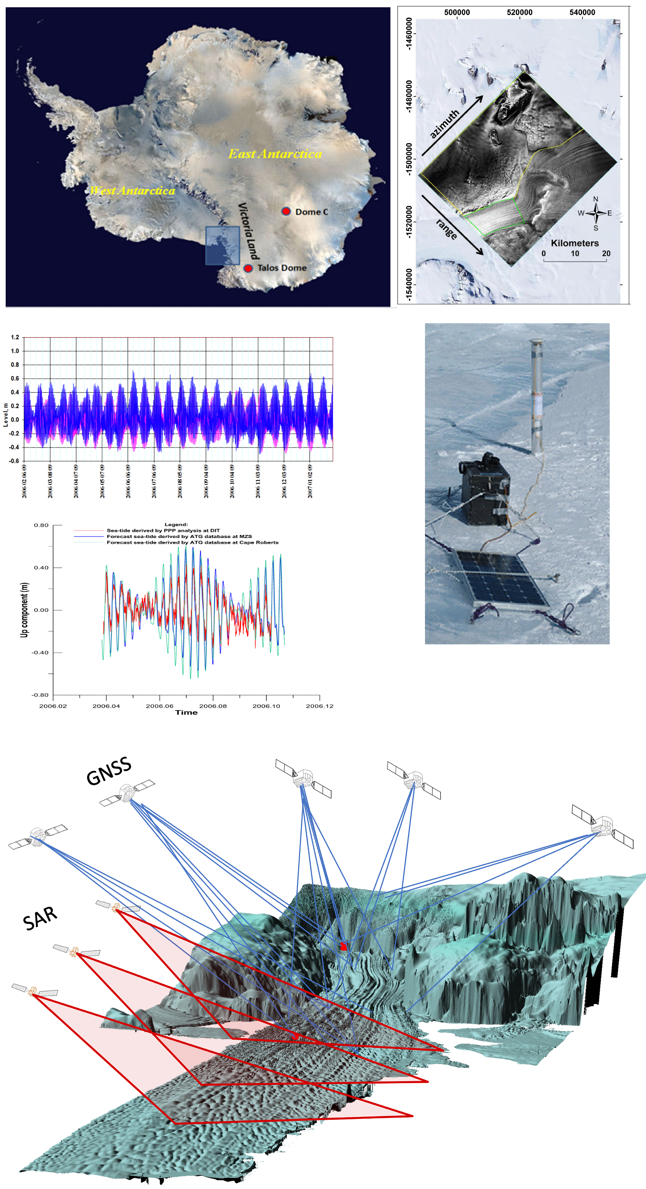
The result of the GNSS data processing is the estimation of the geocentric Cartesian coordinates of stations and their uncertainties expressed within the International Terrestrial Reference Frame 2014 (ITRF2014). The Cartesian coordinates were then converted to a local geodetic coordinate system (North, East, and Up). The time series of the local geodetic coordinates for both stations are shown in
Figure 3, where the trends of the North and East components represent the horizontal velocity of the ice flow, while the Up component represents the vertical motion measured during the 24 days of observation.
The open-source software Tsview, a MatLab program for interactive analysis of the time series based on the least squares fitting technique [
26,
27], was used to estimate linear trends and residual detrended coordinates of time series. The station velocities were then estimated individually for each component from the station position time series.
An interactive inspection of time series was performed to remove some outliers, followed by an automatic outlier rejection using the 3-sigma criterion. The RealSigma noise correlation model implemented in Tsview was used to account for the influence of time-correlated effects in estimating the confidence intervals of the velocity components; finally, the residual time series was estimated after subtracting the trend (
Figure 4,
Table 1).
Spectral analysis of GNSS time series provides a very powerful tool for understanding signals due to the intrinsic mechanism affecting the movements of the stations [
26]. This results in an intuitive means of determining the period of oscillation, but, unfortunately, the total sampling period of 24 days is not long enough to estimate the interesting frequency of 14 days due to the passage of the moon at the equator. Furthermore, the spectral analysis of NEU components was performed only on shorter periods, due to the main diurnal and small semi-diurnal components of the ocean tide, using the Lomb-Scargle periodogram [
27,
28,
29], a statistical tool which can detect and characterize periodic signals in unevenly sampled data. This method evaluates the time series data at the measured time and reconstructs the missing values from the amplitude and phase information of the dominant frequencies, without performing any interpolation [
30]. The results of the analyses are presented in
Figure 4,
Figure 5,
Figure 6 and
Figure 7 and in
Table 2.
The nonlinear motion of the ice flow evidenced by the North component was investigated in more detail, by projecting the components of motion along and across the ice flow direction at DRY1, because the magnitude of the component was not explainable by a simple oscillation of the aluminum pole induced by the ocean tide. In
Figure 5 are reported the components across the ice flow azimuth of 101.17°, measured from the motion profile at the point.
Figure 6 shows the periodograms obtained for time series of both GNSS stations compared with the synthetic ocean tide prediction data.
Concerning point ICF1, the horizontal component EN points out a curved motion of the ice flow where the pole was fixed, and an interesting movement with a saddle shape is evidenced by the Up component.
An important effect that is expected to be present in the David Drygalski movements is the response to ocean wave stresses. However, these vibration resonance frequencies, described, for example, for the ice tongue of the Mertz glacier, are on the order of 10s [
32]. This is too short a period to be highlighted by the spectral analysis described above, due to the sampling rate of the GNSS measurements analyzed.
3. SAR Data Analysis
Although the GNSS time series analysis is very accurate, it refers to isolated points, and therefore it was considered interesting to broaden the analysis in spatial terms also, using synthetic aperture radar (SAR). The processed dataset analyzed consists of 5 Cosmo-SkyMED Stripmap scenes (in the following CSK), made available by the Italian Spatial Agency (ASI) in the framework of the Announcement of Opportunity 2288.
The CSK sensor acquired in X band, with a wavelength of 3.1 cm, and a nominal spacing of 1.54 × 2.35 m, respectively, in range and azimuth. These scenes were acquired in descending geometry from August to September 2009, allowing the formation of three pairs, each with a temporal baseline of 8 days (
Table 3).
Due to the high differential kinematics of the glacier (faster at the center than at the sides, with stable rocky outcrops on the flanks), it is arduous to retrieve displacement velocities considering the unwrapped SAR phase, because of the lack of both sufficient coherence (even with a short temporal baseline) and of reliable ground control points for phase calibration.
An alternative approach is coregistration offset tracking (coherence tracking), less accurate than InSAR but with the benefit of also allowing observation in the azimuth direction [
33].
All the pairs were processed with a DEM-assisted coregistration [
34], considering a DEM previously obtained by processing two ERS tandem pairs (in the framework of ESA Cat.1 project 5410), whose height accuracy and spatial sampling have been deemed suitable to avoid topographic residuals. To mitigate errors related to acquisition geometry, offsets along the glacier were calibrated applying polynomials whose coefficients were estimated through a least square regression of “stable” point offsets (e.g., rocky outcrops where high coherence was retained). In summary, since glacier offsets are expressions of both ice velocities and errors, considering stable point offsets allows splitting these two components (for a review of this technique refer to Liu et al., [
35]).
In general, the precision of tracking-based methods depends on the pixel dimensions: in case of SAR coherence tracking, for the image-patch sizes and oversampling factors considered in this study, the accuracy is of about 1/20 of pixel dimension. The precision of the displacement vector can be approximated to the sum of the accuracies in ground-range and azimuth directions, so, a value referring to a single day is given by the division by the number of days between the two acquisitions [
33]. Knowing the acquisition geometry, local topography, and simulated tide heights, it is possible to decompose the displacement vector into its horizontal and vertical components [
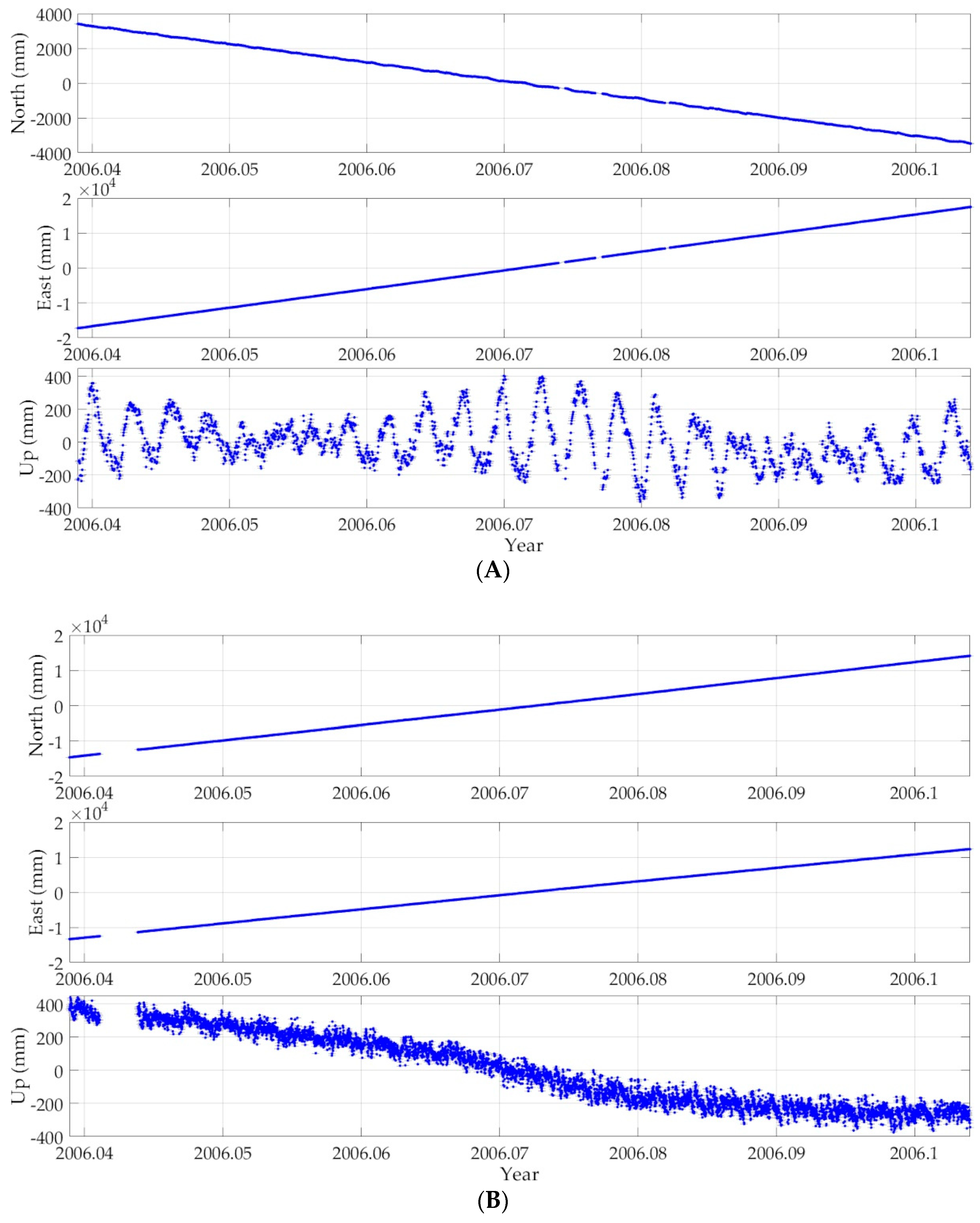
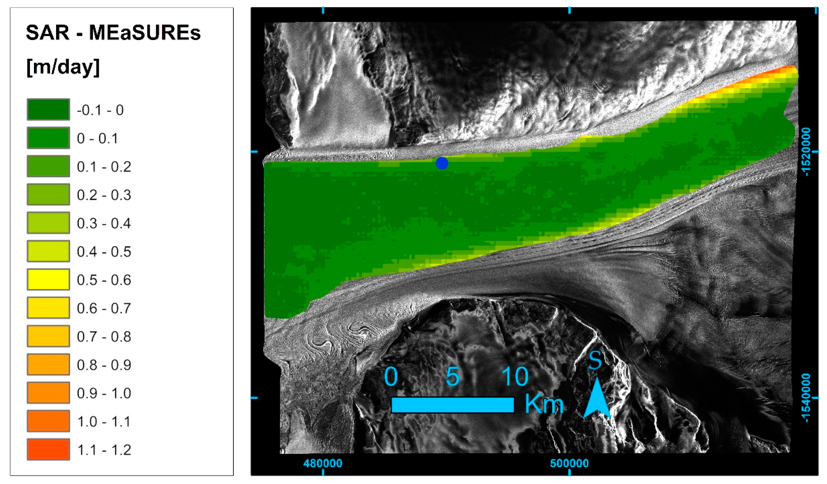
36]. Regarding the subsequent processing, we considered only the horizontal component. Offsets have been interpolated with a natural neighbor algorithm to get a continuous map of the glacier velocity field; then the obtained grids were validated in a GIS environment, comparing the obtained results with respect to the velocities reported in the MEaSUREs InSAR-Based Antarctica Ice Velocity Map, Version 2 [
13,
18,
37,
38,
39].
As a result, the differences with respect to the MEaSUREs velocities are on the order of a few centimeters/day, and the angular direction is consistent with the geomorphological control given by the main direction of the glacier flow (
Figure 8).
Moreover, the offset tracking velocities of the three SAR pairs were also validated with respect to the DRY1 GNSS point, as shown in the
Table 4.
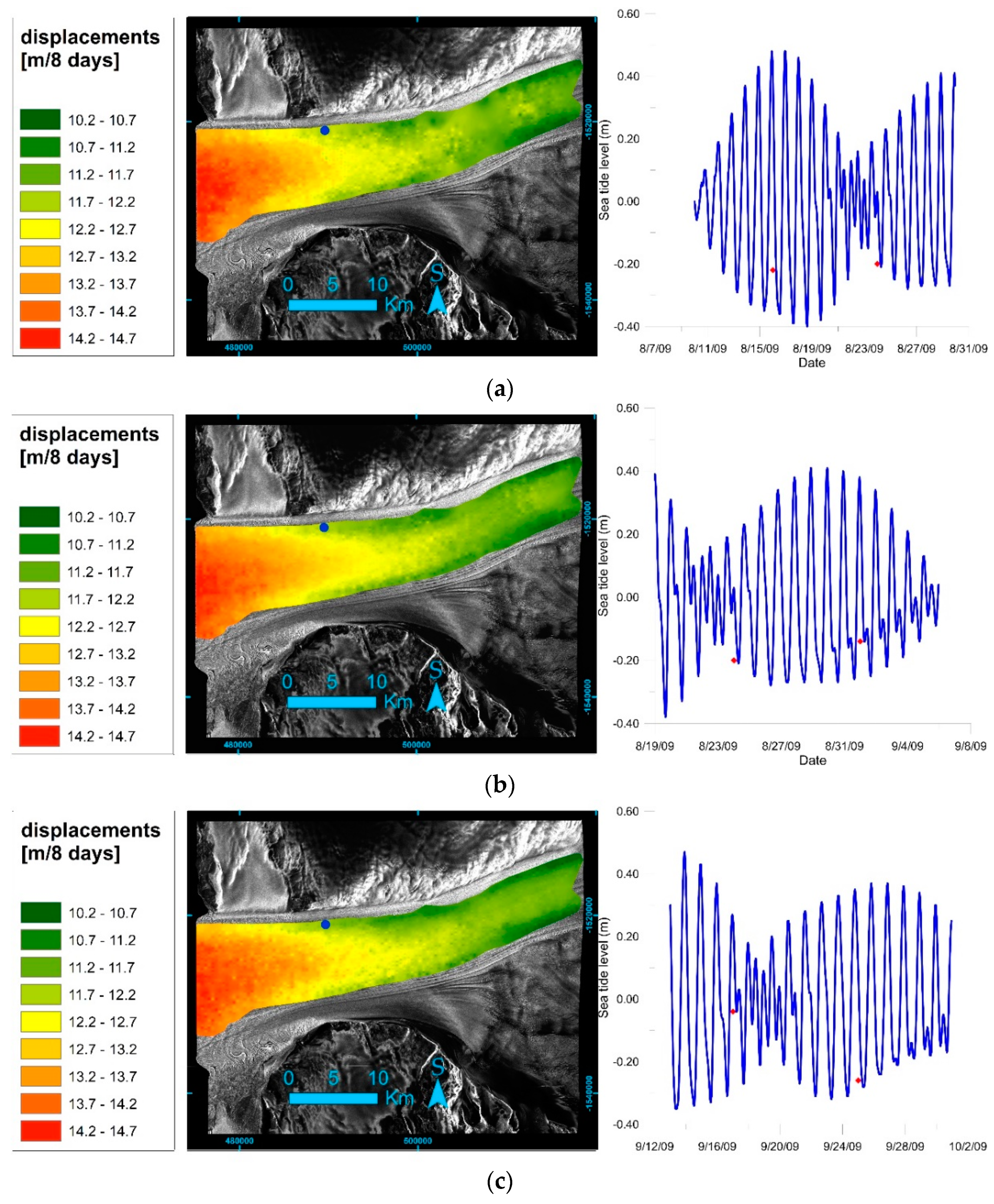
In
Figure 9a–c are reported the estimated horizontal velocities derived by interpolating the SAR offset tracking values of the three pairs, along with the predicted ocean tide in the period corresponding to the acquisition of the master and slave scene of each image pair.
5. Discussion
The analysis of the time series of the two GNSS stations can provide useful information on the movements of floating and grounded parts of David Glacier, both considering the total analyzed period and a daily scale. From the time series shown in
Figure 3 and
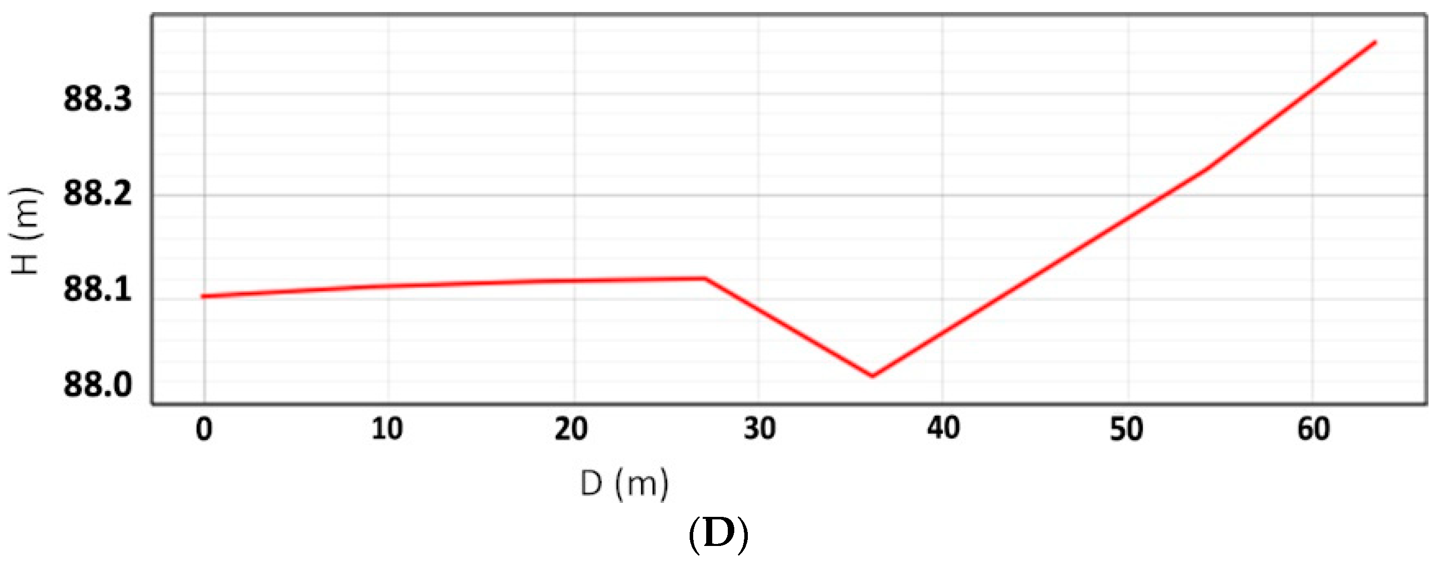
Figure 4, the two GNSS stations have significantly different oscillatory movements due to the locations of the two stations on the glacial tongue with respect to the grounding zone. The DRY1 station points out a horizontal velocity slower than the ICF1 (respectively, 543.447 m/yr ± 0.026 m/yr and 591.964 m/yr ± 0.021 m/yr), and it shows a clear vertical ocean tide signal, but with reduced amplitude, when compared with the predicted one at the same location. ICF1 shows a very small tidal signal at the daily scale in the three components and shows a clear change of horizontal ice flow direction following the constraints of the fjord geometry. A possible explanation for the “saddle” vertical behavior of the point, compared with the local slope of REMA, is that the ice flow from the plateau could encounter a morphological change in the bedrock interface.
In the paper Frezzotti et al. [
39], the velocities measured in the period December 1991–January/February 1994 of a series of points surveyed using GNSS are reported. One of these points (DA2) was in 1994 at a distance of 135.55 m from point DRY1, with an azimuth almost transversal to the point analyzed in this paper (92.47°N). In the period 1991–1994, the published velocity was 533.38 m/yr with an azimuth of 101° against values measured in 2006 through the analysis described here of 543.447 m/yr with an azimuth of 101.17°N. As can be seen, the direction has remained almost constant, although, in the first case, the velocity was averaged over several years in different seasons, and the velocity was higher than 10.07 m/yr in Antarctic summer 2006 with respect to the velocity during 1991–1994. It is not possible from the dataset analyzed in this context alone to understand whether it is a seasonal variation or an overall increase in meridional ice flow velocity, and further measurements would be required.
The ice tongue flows essentially along an E-SE direction; DRY1 shows daily East and North components in phase opposition with respect to the Up component (
Figure 4). The rising of the ocean tide even increases the movement component of DRY1 orthogonal to the main flow direction, which cannot be explained simply by a vertical oscillation of the aluminum pole caused by a transversal change in the glacier slope. In fact, the effects are greater than what might be expected if there were a lateral constraint caused by the anchoring of the ice to the fjord wall and a free vertical oscillation due to ocean tide in the floating part of the tongue, considering the arm of the GNSS antenna pole as leverage. For example, starting from the behavior of the component orthogonal to the ice flow at DRY1 described in
Figure 4, during the maximum tidal excursions, the horizontal variation orthogonal to the flow is about ±6 cm; considering the height of the pole of about 2 m out from the ice, in the case of a rotation instead of a horizontal movement, the effects should require a rotation of the ice surface of about ±2°, which, even in presence of fractured ice blocks of a few hundred meters, would require ocean tidal excursions of several meters. During the phase of greatest tidal excursion (14-day period), an increase in the horizontal ice flow following an increase in the ocean tide amplitude can be observed, but, at daily level, the maximum horizontal velocity it is often observed during the low-tide phase; this effect is in accordance with the direction of seawater outflow from the fjord into the ocean and could also be linked to the constraints of the ice flow driven by gravity [
41,
42,
43].
Analyzing the horizontal velocities at ICF1 and DRY1, a sinusoidal residual signal is highlighted in the detrended time series of movement differences, which could be induced by the torsional motion of the ice flow due to the outflow from the neck of fjord at ICF1 and by the strong confinement induced at DRY1 by the pressure of the northern stream fed by the Talos Dome.
Concerning the SAR data processing, even though the scenes were all acquired at the same time, about 06:15 UTC, corresponding to a low tide condition, their position in the tidal cycle is different, as shown in
Figure 9.
This means that, at the time of the SAR scene acquisition, the glacier is always grounded, but in the time span between on acquisition and another one, its floating time varies depending upon tidal conditions. Starting from this consideration, it is possible to hypothesize that, in the time span corresponding to the temporal baseline of the SAR pairs, the horizontal velocity of the glacier should be greater when the glacier remains floating for longer, since high tide tends to uplift the glacier from the bedrock, and so, due to decreasing basal friction, its horizontal velocity increases. To check this hypothesis, we compared the high tide total height with respect to the summation of horizontal displacements. The high tide total height was calculated with the Cavalieri-Simpson formula [
44] applied to predicted ocean tide at the DRY1 point location; in other words, the analysis corresponds to the mathematical integration of the height in every positive tide condition. A positive correlation between tide heights and velocity becomes clear starting from a tide threshold of 10 cm above the sea level (
Figure 12).
This correlation is verified both for the whole glacier region included in the SAR scenes and for an area of 12 km surrounding the point DRY1. Unfortunately, the few numbers of processed SAR pairs allow neither deriving a conclusion nor attempting a correlation with the GNSS time series.
6. Conclusions
The Drygalski ice tongue interacts with the southern coast of Terra Nova Bay and has an important role in the formation of the polynya, resulting from the action of strong persistent katabatic winds which inhibit the formation of sea ice in the bay and, at the same time, induce the ice formation process beyond this area due to persistent cooling of the water surface [
42]. In addition, Drygalski, with its giant length towards the sea, forms a physical obstacle to the entry of sea ice into Terra Nova Bay from the south. Various authors, e.g., [
3,
7,
11], observed that, even in the presence of a strongly segmented surface of the floating tongue, the main calving events are of large dimension, also connected to collisions with big icebergs (such as B15A) which significantly affect the tongue length. Precise measurements of ice flow velocities are particularly useful for understanding the equilibrium length of the tongue itself. Among these, geodetic GNSS measurements are the best ground truth constraints to be used for surveys extended at the areal level, conducted with remote sensing techniques such as satellite image feature tracking or SAR interferometry.
The analysis of the time series of the GNSS stations DRY1 and ICF1 has highlighted different behaviors, strictly dependent on their position on the ice tongue with respect to the grounding zone, the ocean tides, the morphology of the bedrock, and the fjord geometry. In general, the main daily signal is related to the tidal constraint, which produces changes in the ice flow velocities inversely proportional to its amplitude. During low tide, the velocity of the ice flow reaches its daily maximum, in accordance with the direction of seawater outflow from the fjord into the ocean. In contrast, the inflow of sea water during the rising of the ocean tide level is characterized by an opposite movement to the outflow of the ice towards the sea. During the phase of greatest daily tidal excursion, an increase in the horizontal ice flow velocity can be observed. This could be explained by longer periods of seawater presence at the bedrock-ice interface in the grounding zone, with respect to the phases of small daily ocean tidal excursions.
DRY1 demonstrates a clear response of the floating ice tongue to tidal forces, while ICF1, located close to the grounding zones, shows a very limited daily vertical amplitude of movements induced by the ocean tide.
The small oscillating components observed within the southern flow in a transversal direction with respect to the main longitudinal flow is not easily interpretable on the basis of only 24 days of GNSS observation and would require a longer acquisition at different points of the David Glacier and the Drygalski ice tongue to identify the principal causes of what was observed.
All processed SAR scenes were acquired at the same daily time, corresponding to the low-tide condition, in which the threshold of the grounding zone is supposed to lean against the bedrock. However, in the time span between scene acquisitions there were also tidal peaks, which facilitate the movements of the glacier. The comparison between the integral of tide height computed over an 8-day period against the summation of the horizontal displacements obtained by SAR offset tracking shows a positive correlation becoming clear from 0.1 m above sea level, while below this threshold it is assumed that the movement of the glacier is constrained.
In particular, the DRY1 GNSS time series highlights that, on a daily basis, the horizontal velocity of the pole on which the antenna was positioned increases in correspondence (with a delay of about 3 h) with low tide conditions, in accordance with the direction of seawater outflow from the fjord into the ocean and with a topographic gradient effect, while the SAR processing shows that, over an 8-day period, the overall horizontal velocity of the acquired portion of the glacier increases when it is released from the bedrock, i.e., in tidal conditions higher than a threshold of 10 cm above the sea level.
The variations in the strain pattern of the floating ice tongues can be induced by the formation of basal channels which are also located on the lower side of the David Drygalski [
3]. These channels can be explained by increased melting at the ice-ocean interface [
45,
46,
47,
48], and in some cases subglacial channel outflow can go beyond the grounding line [
12,
48].
Chen et al. [
49], reveals a complex model for the definition of grounding line, which is inconsistent in position with respect to simple tidal forcing and which presents migrations of the grounding line within a large grounding zone. This phenomenon is influenced by numerous factors, including, for example, the hardness of the bed and the presence of subglacial channels. Given that, for the David-Drygalski, as previously indicated, at least three main subglacial channels have been identified, there could be a phenomenon of inland sea water trapping. Even in this area, the position of the grounding line should perhaps be assumed not to be fixed. But to deepen this aspect for the grounding zone of the David Drygalski, further investigations would be necessary, through long time series of altimetric data straddling the grounding zone.
The position of the GNSS points ICF1 and DRY1 is lateral southward, in a higher altimetric position based on the description provided by the DEM REMA, with respect to the three subglacial channels identified in Indrigo [
3]. Two of these are located within the southern flow of David Glacier, and it has been hypothesized that they may reach the grounding line. In this case, the inflow and outflow induced by tidal level variations, which leads to the observation of significant surface velocity variation signals measured daily at the GNSS points, could have reciprocal correlations with the presence of the two subglacial channels.


