Monitoring and Mapping Floods and Floodable Areas in the Mekong Delta (Vietnam) Using Time-Series Sentinel-1 Images, Convolutional Neural Network, Multi-Layer Perceptron, and Random Forest

Abstract

The annual flood cycle of the Mekong Basin in Vietnam plays an important role in the hydrological balance of its delta. In this study, we explore the potential of the C-band of Sentinel-1 SAR time series dual-polarization (VV/VH) data for mapping, detecting and monitoring the flooded and flood-prone areas in the An Giang province in the Mekong Delta, especially its rice fields. Time series floodable area maps were generated from five images per month taken during the wet season (6–7 months) over two years (2019 and 2020). The methodology was based on automatic image classification through the application of Machine Learning (ML) algorithms, including convolutional neural networks (CNNs), multi-layer perceptrons (MLPs) and random forests (RFs). Based on the segmentation technique, a three-level classification algorithm was developed to generate maps of the development of floods and floodable areas during the wet season. A modification of the backscatter intensity was noted for both polarizations, in accordance with the evolution of the phenology of the rice fields. The results show that the CNN-based methods can produce more reliable maps (99%) compared to the MLP and RF (97%). Indeed, in the classification process, feature extraction based on segmentation and CNNs has demonstrated an effective improvement in prediction performance of land use land cover (LULC) classes, deriving complex decision boundaries between flooded and non-flooded areas. The results show that between 53% and 58% of rice paddies areas and 9% and 14% of built-up areas are affected by the flooding in 2019 and 2020 respectively. Our methodology and results could support the development of the flood monitoring database and hazard management in the Mekong Delta.

1. Introduction

Among natural disasters, floods are considered one of the greatest threats, the frequency of which is expected to increase in the future due to urban development and climate change [1]. Southeast Asian countries are particularly vulnerable to flooding hazards, especially during the wet season. Organizations such as the Mekong River Commission (MRC) and the Asian Disaster Preparedness Center (ADPC) are therefore implementing regional flood forecasting systems by synergistically combining hydrological data and modeling outputs [2]. Nowadays, satellite data have become an important component of environmental risk management through flood extent mapping. The latter—flood extent mapping- is a process used to identify the land areas impacted by flooding. At the same time, the production of land use/land cover (LULC) maps has become a frequently used method for flood risk monitoring [3,4]. These maps can be integrated into flood databases to identify risk zones and determine levels of vulnerability.

Floodable zones have become a considerable socio-economic issue at the local level of the Mekong Delta, which is ecologically, economically and socially important, thus many studies have been conducted over the years using Earth Observation data specially to characterize the rice crop. The majority of these studies have focused on delineating the distribution of rice crops using either optical satellite imagery (passive sensors) [5,6] or radar satellite images (active sensors) [7,8,9]. Active or passive sensors used for flood risk applications cover a very wide range of the electromagnetic spectrum, and information from these spectral ranges or their combination contributes significantly to forecasting and risk management. Unlike passive sensors (optical), which are severely affected by cloud cover, an obstacle to environmental studies in tropical and equatorial areas, satellite-based Synthetic Aperture Radar (SAR) can penetrate clouds. Thus, SAR is an interesting source of information for flood monitoring and soil moisture studies. SAR (post-2000), ALOS (L-band, Japan, 2006), TerraSAR-X (X-band, Germany, 2007), RADARRSAT-2 (C-band, Canada, 2007), COSMO-SkyMed and Sentinel-1 (C-band, European Union, 2014) offer new avenues of research, including high spatial resolution (metric resolution) and coherent polarimetric data, in flood management and sustainable development. With a higher temporal resolution than previous SAR instruments, Sentinel-1 is able to monitor the seasonal cycle of water cover every six days. These latest advances in SAR data acquisition have enabled the development of near real-time and automated flood mapping [10,11,12]. Indeed, the possibility of fully automated services for surface water [12] has been investigated and several works have focused on the mapping of the extension of flooded areas and the application of automatic methods using satellite images [13,14,15,16,17]. However, at the present time, Sentinel-1 C-band images for flood mapping have not yet been used in an exhaustive manner.

In addition, the low backscatter value of water, in the absence of wind effects, is frequently used for the detection of flooded areas on radar images. Water surfaces constitute a specular reflector of the radar pulse, which results in a reduced signal returning to the satellite [18,19]. However, rain and wind can increase the roughness of the water surface, backscatter the SAR signal and mask flooded areas. [18,20]. The backscatter of the SAR signal also varies with the angle of incidence (AI) and variations in the local angle of incidence (LIA) due to target topography and AI. [21]. Thus, the backscatter intensity can be influenced by environmental conditions such as landscape topography and shadows.

Another possible difficulty is the identification of flooding in areas where objects protrude above the water surface and thus interact with the radar signal. As such, it is difficult to determine a general threshold for backscatter. The environment can play a very important role in this. For example, water can be masked by vegetation cover, with lotuses and aquatic grasses resulting in uncertainty in mapping the extent of flooding. According to some authors [22], there are normally large areas of widespread aquatic grasses and lotus lakes during the flood season.

In the field of flood mapping, several methods have been applied using satellite images: photo-interpretation and image segmentation, which use mathematical principles such as edge detection, and fuzzy logic with artificial neural network exploration. The most frequently used method is thresholding, which is used for the analysis of SAR images in order to discriminate between the water and non-water areas. These techniques include the following: image histogram thresholding [17,23,24], image classification algorithms [25,26,27,28,29,30] image texture algorithms [31] and, multi-temporal change detection methods [28,29,32,33]. The scientific community agrees that machine learning (ML) methods have several advantages in environmental applications, such as improved mapping accuracy, reduced computation time and reduced model development cost [34,35,36,37]. According to several studies, ML has the potential to fundamentally improve future flood risk and impact assessments [38,39,40,41]. Moreover, recent developments in ML, especially neural network models, have made advanced applications in the field of environmental and risk analysis possible. Applications of ML methods to flood mapping have emerged in recent years [4,42]. Furthermore, CNNs have demonstrated excellent performance in various domains, including image classification [43], object-based image analysis (OBIA [44]) and, scene labeling [45], in the field of computer vision [46,47,48]. Nemni et al., 2020 [49] proposed a CNN-based method for isolating flooded pixels from Sentinel-1 images without any optical band and with minimal preprocessing. Li et al., 2019 [50] evaluated the role of interferometric coherence in urban flood detection using multi-temporal TerraSAR-X data. They introduced an active self-learning convolutional neural network (A-SL CNN) framework to mitigate the effect of a limited annotated training data set. Kang et al., 2018 [51] applied a fully convolutional network (FCN) based on the classical FCN to flood mapping using Gaofen-3 SAR images in China. Shen et al., 2019 [52] developed a near-real-time (NRT) flood mapping system, named RAPID, based on dual-polarized SAR data.

Overall, the present study puts in place a methodology of mapping the floodplain and its land use—in this case, rice paddies—before, during and after the floods and aims to map the fluctuation of the flooded areas. Specifically, it explores the potential of several robust ML models, namely CNN, MLP and RF, by comparing the accuracy of predictive models for flood and floodable area mapping in a complex deltaic environment (An Giang province, Mekong Delta). Moreover, this study attempts to analyze the contribution of Sentinel-1 SAR data in vertical and horizontal polarization, VV and VH, according to backscatter characteristics. Furthermore, based on the results of a comparative study between the optimized ML models, this paper proposes an accurate method for deriving complex decision boundaries between flooded and non-flooded areas and producing reliable detection and mapping of LULC classes that can be potentially impacted by floods.

2. Materials and Methods

2.1. Study Area, Rice Paddies and Hydrometeorological Regime of the Mekong River

2.1.1. Study Area

The study area is located in the Mekong Delta, between 8.5−11.5°N and 104.5−106.8°E in the southern part of Vietnam. Two provinces were studied as folows: An Giang and Dong Thap (Figure 1).

The Mekong is the seventh-longest river in Asia and the twelfth-longest in the world. This great river of Southeast Asia is nearly 4000 km long, has its source on the Tibetan plateau, and crosses China, Burma, Laos, Thailand, Cambodia and Vietnam before flowing into the South China Sea. In the Vietnamese part, the delta covers an area of nearly 40,000 km² in 12 provinces and municipalities inhabited by nearly 18 million people, accounting for 20% of the country’s population. The economy is mainly based on agriculture, fishing and trade.

2.1.2. Rice Paddies

The Mekong Delta is a vast flood plain and one of the most fertile agricultural areas in Asia. Indeed, the south of Vietnam is a large agricultural region that is specialized in the cultivation of rice. In 2020, despite drought and salinization, the Mekong Delta, the breadbasket of Vietnam, produced 24 million tons of rice from its 1.5 million hectares of cultivated land, an average yield per hectare of 6 tons. Rice export from the Mekong Delta amounted to 6 million tons according to Le Courrier du Vietnam, 27 May 2021. The main export markets for Mekong rice are Malaysia, the Philippines and China. Cultivation practices in the Mekong Delta include the traditional method, which involves transplanting and continuous flooding, and the modern method, which involves direct seeding and alternate drying. In the Mekong Delta, there are irrigated rice ecosystems with three main cropping seasons: winter-spring, summer-autumn and autumn-winter [53]. We are more interested in the autumn-winter cropping season. According to the rice cultivation calendar for this season, rice is planted in July-August and harvested in December-January. According to Phan 2018 [47], the autumn-winter crop has the lowest productivity during the wet season.

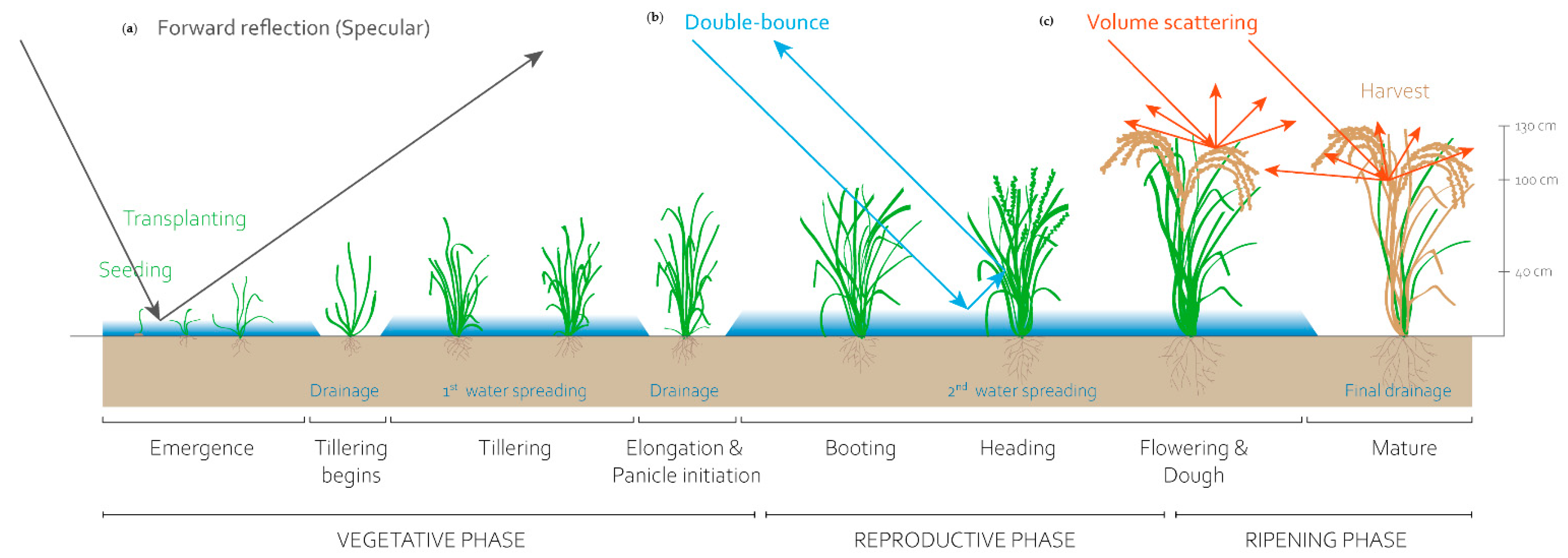
An acceptable estimate of flood-damaged rice must be made. Previous studies have shown that this is not an easy task [54], as permanent water must be distinguished from flood water. SAR data have the specific radar backscatter response of vertically structured vegetation on flooded or wet ground, and thus they have the ability to distinguish rice from other land cover classes. Figure 2 shows three mechanisms that intervene in the analysis of the interaction between a radar electromagnetic wave and the rice: the direct reflection (specular), the double rebound and the volume diffusion.

In the first period (vegetative phase) (Figure 2), the rice fields are covered with water for most of their growing cycle. The fields are only flooded during certain periods (emergence and tillering in the vegetative phase and booting and heading in the reproductive phase). The soil remains wet (not flooded) as tillering begins and during elongation and panicle initiation in the reproductive phase and ripening phase (maturation). Radar backscatter from flooded fields is low due to the specular reflectance of the water surface but is very high throughout the growing period (vegetative to reproductive phase). After this period, radar backscatter increases steadily with the rapid increase in height (up to 100 cm) and biomass of the rice plants. At this time, double bounce is the main backscattering mechanism. The next reproductive phase includes panicle initiation, heading and flowering. During this phase, there is less increase in plant height and therefore less increase in biomass [3,4]. The last phase, maturation, with its milk, dough and ripe grain processes, is characterized by volume diffusion (Figure 2).

2.1.3. Hydro-Meteorological Regime of the Mekong River

The rainfall regime of the region is characterized by an alternation between dry and wet seasons. The period of floods takes place between June and November. It coincides with the arrival of the monsoon, a hot and humid wind coming from the equator which brings abundant rainfall to the entire Southeast Asia region. The monsoon is reinforced by the temperature differential between the continent and the ocean. The region can record rainfall of up to 2000 mm per year. The amount of rain that falls in the region is highly variable depending on time and place. From one month to another, the amount of rainfall recorded can double. In addition to flooding, Southern Vietnam is particularly vulnerable to the effects of climate change. Indeed, the Mekong Delta is located 10 m above sea level, and so it is exposed to marine submersion. Rising sea levels will lead to increased saltwater intrusion into the main branches and channels of the Mekong, which will contribute to crop destruction, reduced yields and soil pollution.

The lower Mekong and its rivers are influenced by the Southeast Asian monsoon. The hydrological regime has very large annual and interannual variations. The monsoon season, which theoretically consists of a dry season and a rainy season (maximum in July), leads to rainfall in mid-April if there is no precipitous thaw, and water in July-August, all with strong year-to-year variations depending on the strength of the wet monsoon. Then there are the convergent rains that extend the rainy season; these result in floods from October to November more consistently. Finally, there are typhoons, which generate their maximum water potential in November-December.

2.2. Data Set

2.2.1. Satellite Data

The data used in this study are images from the Sentinel-1 radar satellite of the European Space Agency (ESA). Launched in 2015, Sentinel-1A and Sentinel-1B, share the same orbital plane, generatinge data in the microwave (long wavelength or microwave) in C band with a wavelength of about 4.5 cm. The images have been uploaded onto the ESA Hub Copernicus platform. They are in Ground Range Detected (GRD) (intensity and amplitude) and are obtained from SLC images (

Table 1. Dataset descriptions.

Attribute Name	Description
Collection	Sentinel 1A/Sentinel 1B
Time period	June to November 2019 and 2020
Level of processing	GRD
Polarization bands	C-band and VV—VH
Orbits	Ascendant/Descendent
Orbit number	18
Spatial resolution	10 × 10
Time resolution	06 days
N° images	60/2019 60/2020

).

The images are downloaded over a period of six months (from 6 June to 30 November), which corresponds to the period of flooding in the Mekong Delta region. The temporal resolution of the Sentinel-1 data is 6 days, which enables the acquisition of 30 images over the study period. The two Sentinel-1 satellites are located in the same orbit at about 900 km above the Earth’s surface. Their phase shift allows for a better temporal resolution. These images in the C band with a wavelength of about 4.5 cm are acquired in two polarizations, VH and VV. For each acquisition, Sentinel-1 generates two bands with a vertical polarization in transmission and a horizontal one in reception, and another vertical in transmission and reception. The polarization of Sentinel-1 is also called monochromatic polarization, which means that we will always obtain the same amplitudes and the same wavelengths. The data were acquired on orbit N° 18, which passes over the Mekong Delta. The number of the orbit is an important parameter as it allows for the acquisition of images of the same area of study and at the same time. However, images are acquired in ascending or descending orbits, and the direction of the orbit is an important parameter for taking into account the interpretation of the images. The characteristics of shots (angles of incidence) also have an impact on the interpretation of images. Indeed, the Sentinel-1 images were acquired with an angle of incidence between 30° and 45°, which means that the first pixels of the proximal range are at 30° and the last pixels of the distal range are observed with an angle of incidence of 45°. This means that two geographical objects of the same nature can have different backscatters depending on their acquisition angle. This can cause problems in interpreting the surfaces studied, especially when working on the entire image.

2.2.2. Environmental Data

Water level data of the Mekong River and diurnal precipitation data from 2019 to 2020 were downloaded from the NOAA (https//www7.ncdc.noaa.gov, accessed on 18 June 2022) and the Mekong River Commission platforms (https://www.mrcmekong.org/, accessed on 18 June 2022) corresponding to the measurement of the hydro-meteorological stations (Figure 2). These data were compared with the backscatter values from radar images acquired for the two years.

2.3. Methodology

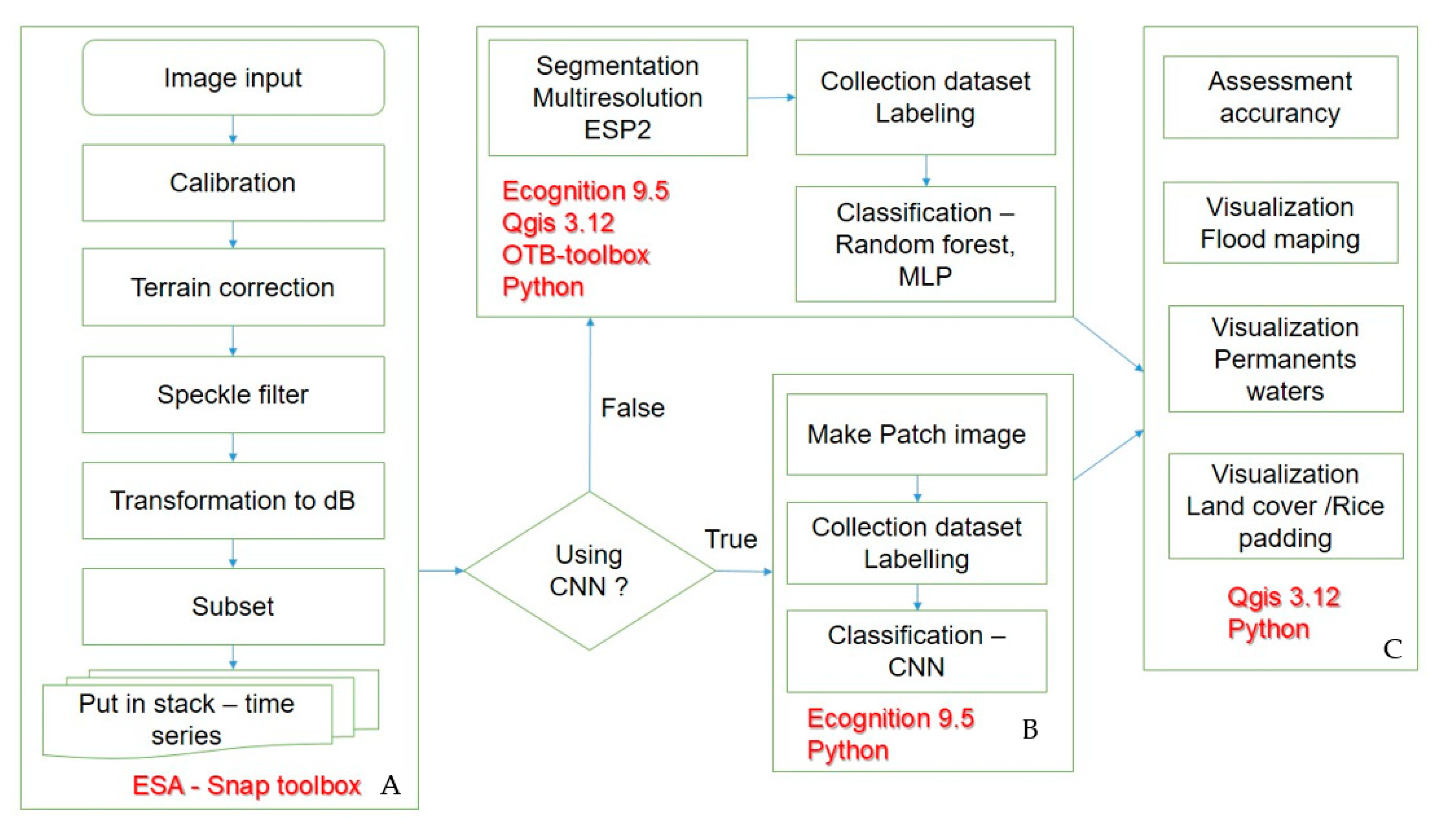
The methodology performed in this study aims, on the one hand, to observe and map the floodplain and its land use—in this case, rice fields—before, during and after the floods, and, on the other hand, to map the fluctuation of the flooded areas. Indeed, image processing was performed in three steps: pre-processing (Figure 3A), image processing (Figure 3B) and post-classification (Figure 3C).

2.3.1. Pre-Processing

After downloading the images, several processes are required to calibrate, filter and geometrically correct them. Calibration is the process of converting digital pixel values to metrically calibrated SAR backscatter. The GRD Sentinel-1 products, which are Level 1 products, have not received radiometric pixel corrections, and so radiometric biases may still be present in the images. In order to convert the intensity into a usable backscatter coefficient and to be able to compare images acquired at different dates, it is necessary to radiometrically calibrate the images. This is a normalization. The calibration allows the intensity of the signal to be corrected according to the characteristics of the sensor and the local angle of incidence. Several calibration options are available as follows: sigma0, gamma0 and beta0. In general, it is best to choose the sigma0 calibration for terrain with little relief, such as the Mekong Delta. The calibration allows the output images to be calibrated in sigma0 VH and VV.

“Terrain correction” processing was applied to allow orthorectification of the image to correct for distortion effects that occurred during image acquisition. This operation also allowed the image to be georeferenced so that it could be projected onto a known terrestrial reference frame (geographic [WGS] or cartographic [UTM]). This operation re-projects the image in the right direction, assigns a projection and corrects any effects related to the terrain. To do this, SNAP software used a DTM (by default, SRTM 3 s) that it downloaded automatically.

A pixel on the SAR image contains a signal with an intensity that corresponds to the backscatter of many reflectors present on the surface imaged by the sensor (Lee et al., 1994a). The total signal contained in a pixel is therefore a coherent superposition of all the contributions of the signals backscattered by each of the surface’s reflectors. The phase of each reflector is correlated with the distance between these reflectors and the satellite as well as with the physical and electromagnetic properties of the reflectors. Thus, this large number of reflectors produces interference between the signals backscattered by each reflector, causing the salt and pepper effect and the salt effect (speckle) observed on SAR images. The filter applied is a convolution window of variable size that reduces noise by smoothing the image values.

The last pre-processing step is the logarithmic transformation of the unit backscatter coefficient converted to dB.

As a result of data preprocessing, there are two datasets for the years 2019 and 2020. The data are a collection of images by the time of the flood season each year (from June to December). To analyze land cover, a machine-learning model was built on a data set consisting of 20 images in June, July, and August. To determine the evolution of the annual flood season, monthly data (from June to December) will be used to create a flood map for each month.

2.3.2. Machine Learning Algorithms (CNN, MLP and RF) and Classification of Flooded Areas and Flood Zones

Image Segmentation and Feature Extraction

Segmentation is defined as the process of dividing images into discrete regions or objects that are homogeneous with regard to their spectral and spatial characteristics [55,56]. In this study, multi-resolution segmentation (MRS; [57]) was applied. Implemented in the eCognition^® software (Trimble Geospatial Imaging), MRS has recently become the best-known algorithm for segmentation. MRS is a technique for merging regions of interest in order to achieve separations that maximize inter-object variability while minimizing intra-object variability. The fusion parameter of these regions is based on a homogeneity criterion resulting from the combination of a spectral criterion and a shape criterion. In total, three parameters are studied for the realization of the segmentation: scale parameter, the weight attributed to the spectral value and the shape of the pixel associations, as well as the weight attributed to the compactness and the roughness of the regions. The scale parameter, which is used to determine the final object size, corresponds to the maximum heterogeneity allowed for the creation of an object [58]. In order to segment the image into objects, MRS relies on a key control called the new scale parameter estimation (ESP). The local variance (LV) parameter capable of detecting scale transitions in geospatial data is the key element in the ESP segmentation algorithm. The tool detects the number of layers added to a project and iteratively segments them in a bottom-up or top-down approach where the scale factor of the segmentation increases by a constant increment provided by the user. The value of the local variance parameter is computed at each iteration and serves as a condition for terminating the segmentation process: when the LV value of a layer under consideration is equal to or less than the value of the previous iteration, the iteration terminates, and the objects in the layer are segmented [55].

A fusion image after preprocessing has a size of 11,961 × 9292 pixels. In this study, MRS extracted geographic image features with the parameters scale = 15, shape = 0.2, and compactness = 0.5 based on an optimization process. The geographic object had characteristic values, in this case the average value per signal band of all pixels belonging to this object. The dataset of objects had hundreds of thousands of objects that were generated after the application of MRS on fusion images. For the training set, labeling objects around the observation points have been collected. Algorithm MLP, RF used this training set for constructing and testing the models.

Table 2. Training set for MLP andRF descriptions.

Class Name	Number of Objects
Water	1065
Rice paddy	1177
Built-in	1109
Garden	1265
Forest	1100
Total	5716

shows the training dataset.

The fusion images with a size of 11,961 × 9292 pixels from the site web of The European Space Agency (https://scihub.copernicus.eu/dhus/, acceded 13 January 2021) has used to train the model; the authors divided the original image into a patch-images set with size 8 × 8 by a function chess-board segmentation of Ecognition@trimple 9.5. Thus, a data set created from an original image has 1,735,695 patch-images. The training dataset is selected based on a set of observation points at the terrain. Each selected patch image must have more than 70% of the pixels whose signal values correlate with one of the observed points (correlation approaches 1). From there, label the patch image as a highly correlated observation point. This labeling job is performed automatically by Ecognition@trimple software version 9.5.

Table 3. Training set for CNN descriptions.

Class Name	Number of Patch-Image
Water	1103
Rice paddy	1520
Built-in	1056
Garden	1504
Forest	1264
Total	6447

shows the training dataset.

In the case of building a flooded areas map (including the canal system and the flooded areas), the authors still use the data in Table 3, with the two classes: flooded areas, and non-flooded areas (the garden, built-in, and rice paddy).

Convolutional Neural Network

Convolutional Neural Networks (CNNs) use a mathematical operation (convolution) to replace general matrix multiplication in at least one of the layers [59]. CNNs have become popular due to their ability to solve classification problems such as image recognition and time series classification. LeCun et al., [60] obtained very good results by using a CNN with a model applying backpropagation. The idea of developing CNNs was initially based on local connectivity, in which each node is connected only to a local region of the input [61]. The resulting network has many connections but relatively few free parameters.

Model Building and Training

The architecture of CNNs is a structure with a series of layers: convolutional layers, grouping layers and perceptron layers. The CNN model proposed in this work is composed of two convolutional layers (Figure 4).

The feature maps are organized into convolutional layers in which each unit is connected to the local patches in the feature maps in the previous layer by shared weight matrices which are called filter banks. The usual size of a filter is 3 × 3, 5 × 5 or 7 × 7 pixels. In this study, a 3 × 3 filter was applied. The new hidden deep layers of neural maps were obtained as a result of repeating matrix convolution on the neural maps. The role of the pooling layer is to merge features into a pixel by maximum or average operations. After a pooling layer, the feature maps are reduced in size, but their basic features are kept for the next step. A CNN compares the images fragment by fragment. The fragments that are searched for are called features. The CNN looks for approximate features that are roughly similar in two different images rather than doing a full frame-by-frame comparison. According to Kim (2017), CNNs can be considered as trainable multilayer feedforward artificial neural networks that include several feature extractions stages. Convolutional layers characterize each feature extraction step with learning filters, pooling layers, and activation functions or nonlinearity layers [62]. Another important element in the process is the rectified linear unit, or ReLU, which replaces negative values of the network being trained with a zero.

Multi-Layer Perceptron

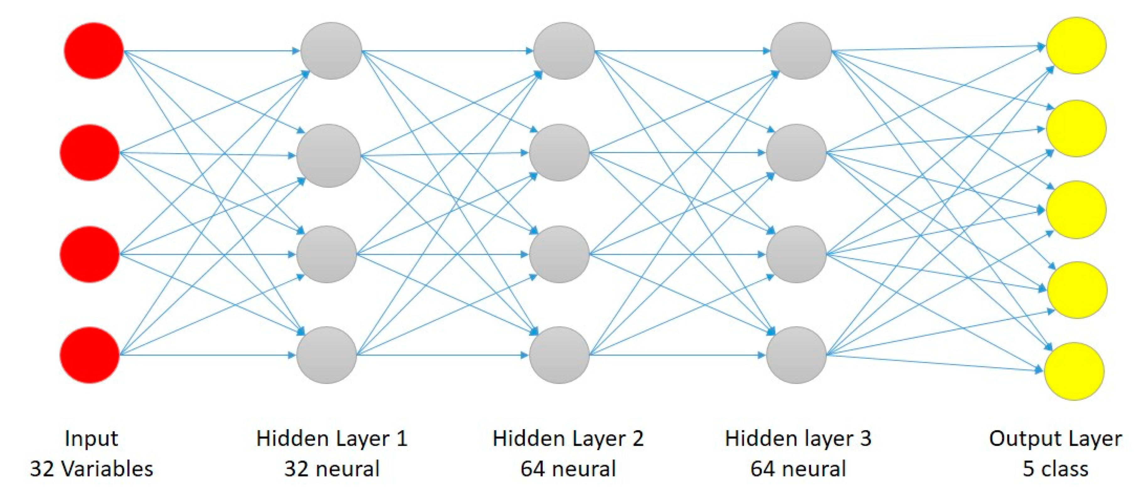
In the field of ML, the perceptron is a supervised learning algorithm for binary classifiers (i.e., separating two classes). It is a type of linear classifier and the simplest type of artificial neural network. The MLP is composed of several units, called neurons, linked together by connections. The MLP is an oriented network of artificial neurons organized into layers in which the information propagates in one direction only, from the input layer to the output layer. The neurons are organized into an input layer, output layer, and one or more hidden layers (Figure 5).

The input layer does not contain neurons. Rather, it is a virtual layer associated with the inputs of the system. The next layers are layers of neurons. In Figure 5, there are 40 strip inputs, with 32 neurons in the 1st hidden layer, 64 neurons in the 2nd, 32 neurons in the 3nd, and 5 land use classes in the output layer. The last layer always corresponds to the outputs of the system, which correspond to the outputs of the neurons. In general, an MLP can have several layers and several neurons (or inputs) per layer. The number of layers corresponds to the number of weight matrices available in the network. A layer is a set of neurons with no connections between them. In MLP, a neuron in a hidden layer is connected as input to each neuron of the previous layer and as output to each neuron in the next layer. The weighted connections link the neurons together. The functioning of the network is conditioned by the weights of these connections. The connections “program” an application from the space of inputs to the space of outputs through a non-linear transformation. The training process goes through two stages, feedforward and backpropagation.

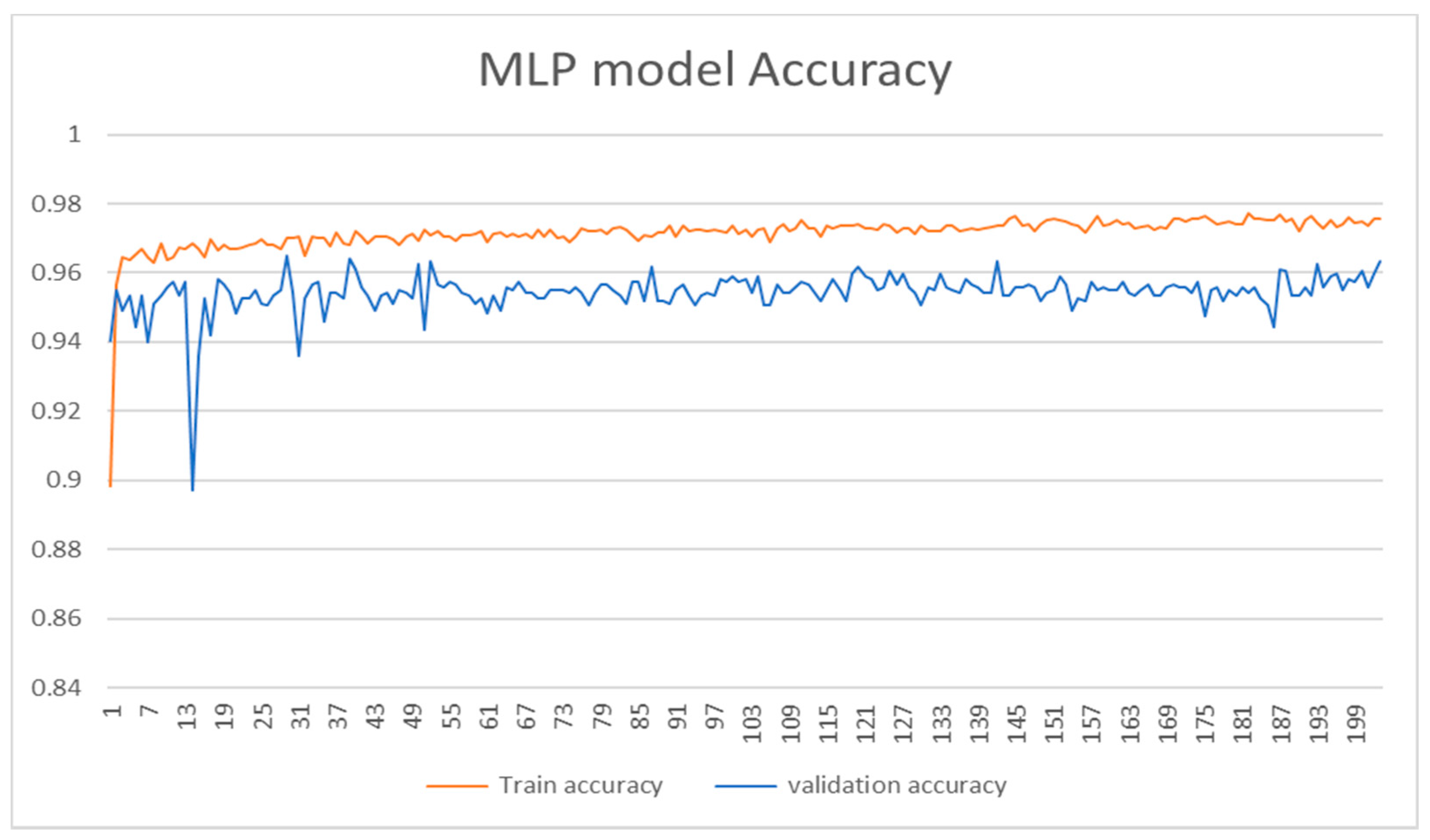
In Figure 6, the MLP model avoids the overfitting error with test—accuracy = 0.9541 and test-loss = 0.1297.

Table 4. The hyper-parameter of MLP.

Layer	Output Shape	Parameter
input	(none, 32)	1312
Hidden Layer 1	(none, 32)	1056
Hidden Layer 2	(none, 64)	2112
Hidden Layer 3	(none, 64)	14160
Output Layer	(none,5)	325
Total params:		8965

show hyper-parameter of a Multi-Layer Perceptron which is descripted in Figure 5.

Random Forest

The Random Forest (RF) algorithm has been widely applied to the classification of floods and floodable areas. It is a non-parametric ML algorithm developed by Breiman [63]. An RF algorithm is constructed with several decision trees based on the bootstrap technique, a statistical inference method that allows for the approximation of the distribution of an estimator when the distribution of the sample is not known. The most important parameters of an RF classifier are the tree depth and the minimum sample size. In this work, 500 trees were established with a subset as the number of features calculated as the square root of the total number of features. The free software Orfeo ToolBox (OTB), in the version integrated with QGIS, was used for this application. In order to train and validate the model on independent data sets, we randomly divided the database into 70% for training and 30% for validation. This algorithm has the advantage of not being influenced by the problem of overlearning that occurs when a model is based too strongly on the training data. This algorithm is frequently used for SAR image classifications, whether in forest areas [64,65] or in crop areas [66].

2.3.3. Accuracy Assessment

Evaluating an ML model is as important as creating it. We created models to run on new, unseen data, and so a thorough and versatile evaluation was necessary to create a robust model. In this work, a normalized matrix was used for this purpose [67]. The confusion matrix was normalized using the number of control points and based on the proportion of classes surface obtained in the classification. Moreover, the raw error matrix was obtained from the validation points. This matrix was normalized to obtain accuracy/error coefficients and statistics (Overall Accuracy [OA], Producer Accuracy [PA], and User Accuracy [UA]). These metrics were applied through the three algorithms to evaluate the performance of the classifications. In general, the OA is expressed as a percentage, and an accuracy of 100% corresponds to a good classification where all reference pixels have been classified correctly. It is calculated by dividing the number of correctly classified pixels by the total number of reference pixels. The PA is a class indicator that characterizes the omission error (PA = 1/omission), while UA is a class indicator that characterizes the commission error (UA = 1/commission). The probability of reference pixels being correctly classified in a searched class is expressed by the PA.

A presentation of the point estimate of precision is made by some studies [68] through the use of the confidence interval. The most commonly used confidence interval is 95% [67,69]. In land cover accuracy assessments, the standard method for constructing a confidence interval is to assume a normal distribution of the point estimate with a standard deviation equal to the resulting estimate of the error margin. In other words, the square root of the estimated variance is divided by the sample size [64]. In this paper, the confidence intervals were automatically calculated in the Python script included in QGIS.

3. Results

3.1. Backscatter Profiles of Rice Fields in the Dry Season and the Wet Season

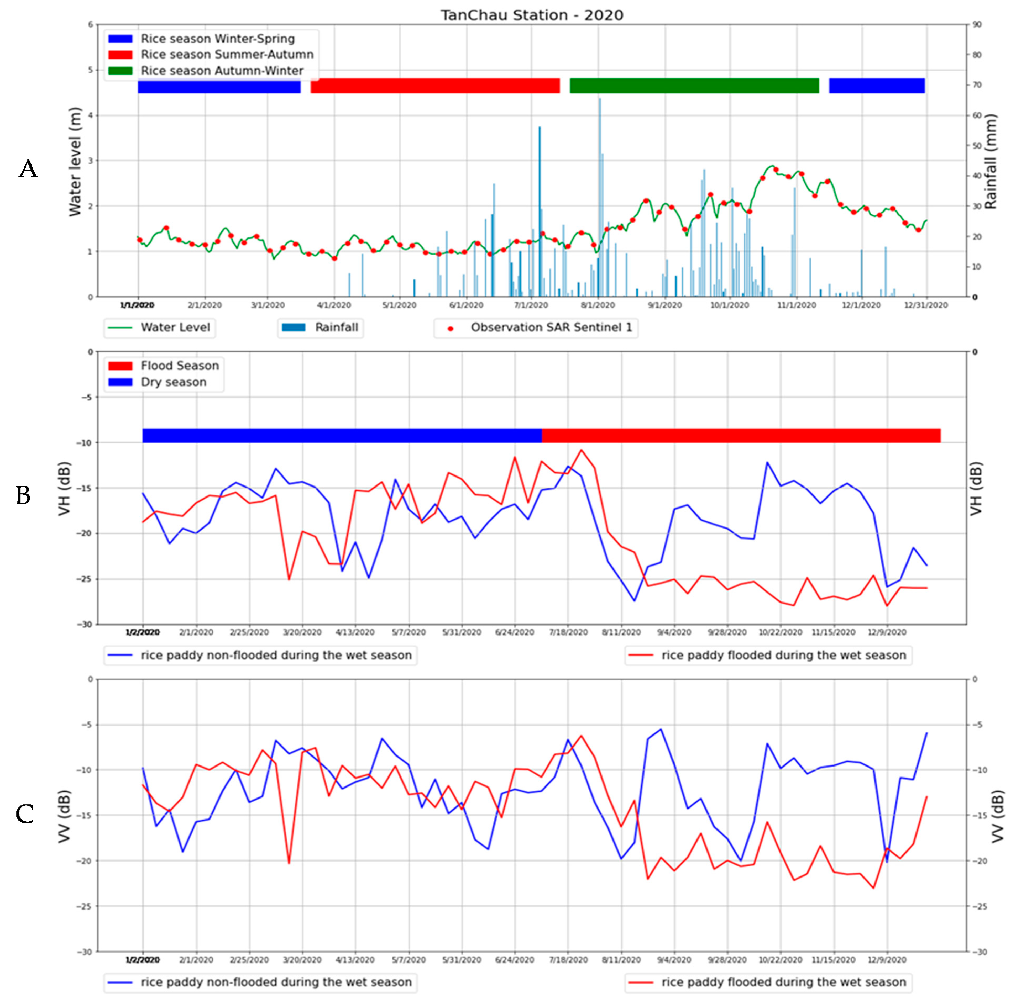
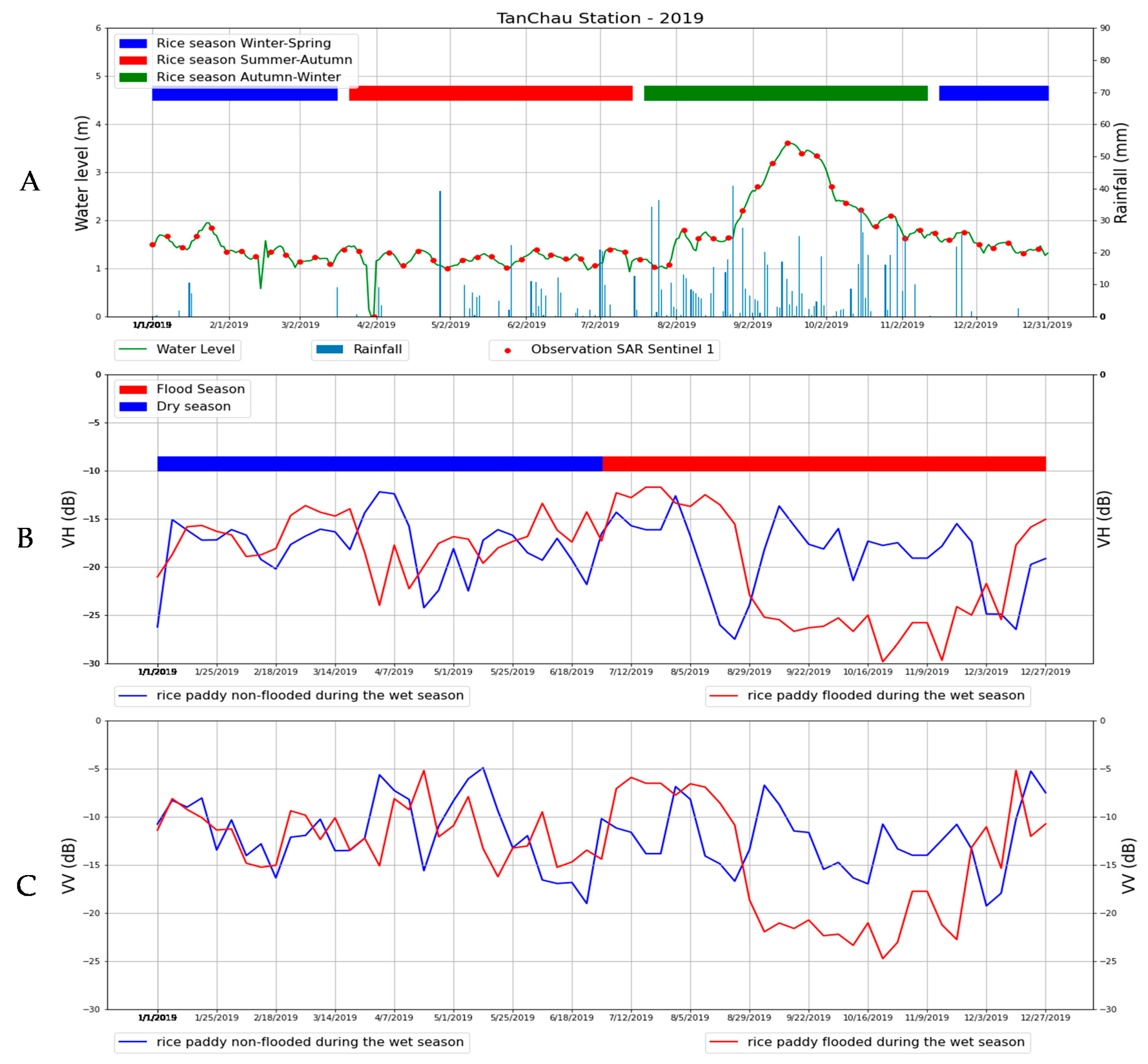
Based on the principle that the radar signal is sensitive to surface moisture, we analyzed the backscatter coefficient of a few different rice paddies for reference during the dry and the wet seasons (flooded paddies and non-flooded paddies) in correlation with the daily rainfall for two years (2019, 2020) recorded at the Tan Chau hydro-meteorological station located in the study area. These data were interpreted in relation to the rice seasons, the SAR Sentinel-1 satellite observations (60 images per year, 5 images per month) and the water levels of the Mekong River as recorded at the same station over the two years. The water levels of the Mekong River started to increase in June along with the increase in rainfall with a maximum of 70 mm on August 1, 2020. The rainfall determined the increase in the Mekong water levels between June and November of both years with a maximum of almost 3 m for 2020 and 3.5 m for 2019 because of the abundant rainfall in the same period.

The backscatter values were lowest for VH (b) and slightly higher for VV (c) in 2020. VH had the largest amplitude and showed significant backscatter peaks, especially for flooded rice paddies. The variation in backscatter coefficient values showed the influence of the surface moisture on the radar signal, namely during the wet season and for flooded rice paddies. For example, for June, the backscatter coefficient values were very low for flooded rice paddies, with values between −25 and −30 db in VH and between −20 and −25 db in VV (Figure 7). The coefficient showed low values until the end of the wet season (November) for the flooded rice paddies. The autumn-winter rice season was dominated in some areas by floods, and this season could therefore be considered less productive. The flooding period that coincides with the autumn-winter rice season should be considered a “rest” period in the rice growing cycle, as it is characterized by reduced rice production.

In the dry season for the two different rice paddies and in the wet season for the non-flooded rice paddies, the variation in the coefficients of VH and VV is explained by the different phenology of the rice. A rice cycle generally has three main stages: the vegetative phase, the reproductive phase and the ripening phase. Before transplanting, rice paddies are usually flooded for several weeks to prepare the soil (i.e., to make the soil very soft and to level the field). The rice plants are then planted in the flooded soil under 2–5 cm of water. The VH and VV backscatter values were relatively low during this transplanting period (December to January; between −20 and −22 db for the VH and between −15 and −20 db for the VV) for the first crop and July to August for the second crop (−27 for the VH and −25 db for the VV) because of the smooth water surface (forward reflection [specular]). After transplanting, the rice plants begin to grow by developing tillers and leaves, the initiation of panicles. At this stage, the height of the plants and their biomass become important. The rice plant has reached the heading stage when the panicle is fully visible. The backscatter intensity for both polarizations increased during February-March (−12 db for both polarizations) and June-July (−11 db for the VH and −6 db for the VV) due to changes in the roughness of the rice paddy surface. The rice showed two peaks indicating the two heading dates of the first and second crops, respectively. The first peak was often between late May and early June, while the second peak appeared in October. The flowering phase begins after the end of the heading phase, which is characterized by the cessation of the development of plant height and biomass and the reduction in the water content of the leaves and stem. During this phase, the intensity of backscatter values also decreased. After harvest, the fallow period rice fields were either bare or sparsely covered with weeds, resulting in a significant decrease in backscatter values (−25 db in VH and −20 in VV for early March and −27 db for the VH and −20 for the VV for early August). In a general way, for non-flooded rice fields, VH and VV showed an increase in backscatter coefficient values for the vegetative and reproductive periods of all three rice seasons, and of two rice seasons for the flooded rice paddies. The low values of the coefficients for both polarizations (−25 db for the VH for the flooded fields and −20 db for the VV) for the two types of rice fields during the dry season correspond to the harvesting of the rice paddies (Figure 7).

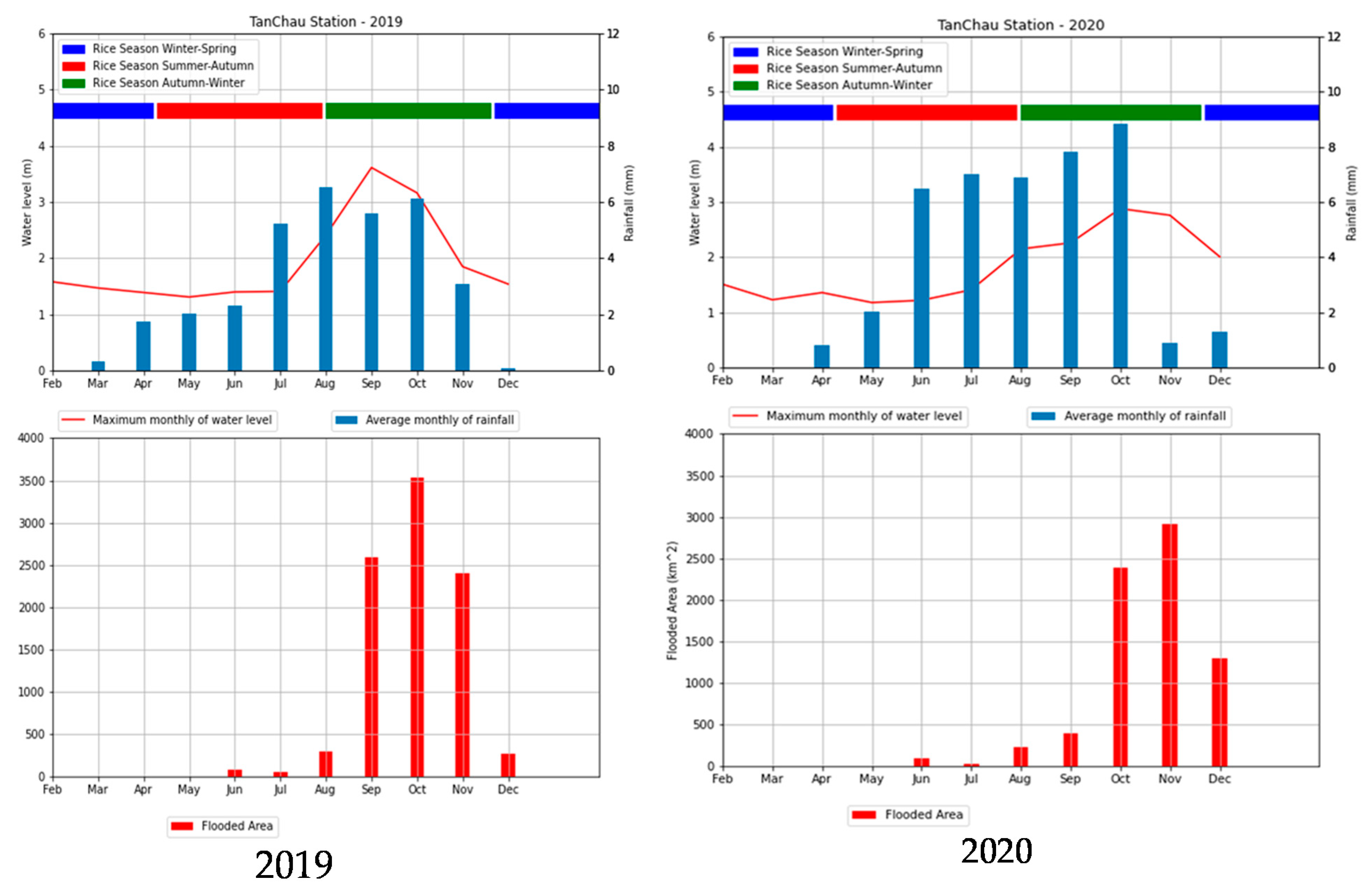
In 2019, according to Figure 8, the rainy season started later (end of June) and ended earlier (November). On the other hand, the maximum rainfall did not exceed 45 mm, and the highest amounts were recorded in August. The maximum level of about 3.5 m was recorded in mid-September. The backscatter values were lowest for VH (b) and slightly higher for VV (c) in 2019, as it was the case for 2020. The high backscatter coefficient values correspond to rice paddies with advanced vegetative development (high chlorophyll activity values). As with the year 2020, for all the reference rice paddies, the backscatter coefficient was found to increase progressively during the rice growth phase in all three seasons for the non-flooded rice paddies in the wet season and in two seasons for flooded rice paddies in the wet season. The two polarizations illustrate this sensitivity of the radar signal to rice growth. In addition, we also noted that the radar signal is sensitive to harvesting time: a decrease in the signal was observed after harvesting (Figure 9).

3.2. Model Validation and Comparison

An evaluation of the model performance with the validation and training data set was performed in order to find the optimal classification model based on its generalization ability. To evaluate the performance of all the methods, the statistical criteria of Overall Accuracy (OA) (

Table 5. OA and uncertainty of CNN, MLP and RF classifiers by month for the wet season.

	CNN Overall Accuracy (OA)
Month	2019		2020
	OA	Uncert	OA	Uncert
June	99.81	±0.01	99.66	±0.01
July	99.31	±0.03	99.68	±0.01
August	99.13	±0.02	99.62	±0.01
September	98.67	±0.02	99.87	±0.01
October	98.67	±0.02	99.51	±0.01
November	98.64	±0.02	96.51	±0.03
December	99.09	±0.01	99.35	±0.01
	MLP Overall Accuracy (OA)
Month	2019		2020
	OA	Uncertainty	OA	Uncertainty
June	97.57	±0.01	June	97.57
July	98.01	±0.02	July	98.01
August	97.12	±0.03	August	97.12
September	98.43	±0.01	September	98.43
October	96.18	±0.04	October	96.18
November	96.98	±0.02	November	96.98
December	95.53	±0.03	December	95.53
	RF Overall Accuracy (OA)
Month	2019		2020
	OA	Uncertainty	OA	Uncertainty
June	99.68	±0.01	June	99.68
July	98.87	±0.02	July	98.87
August	97.92	±0.03	August	97.92
September	99.43	±0.01	September	99.43
October	97.18	±0.03	October	97.18
November	94.98	±0.03	November	94.98
December	92.53	±0.02	December	92.53

) and Producer Accuracy (PA) (

Table 6. PA and uncertainty of CNN, MLP and RF classifiers by month for the wet season.

	CNN Producer Accuracy (PA)
Month	2019				2020
	Flooded		Non-Flooded		Flooded		Non-Flooded
	PA	Uncert	PA	Uncert	PA	Uncert	PA	Uncert
June	94.78	±0.2	99.98	0	90.25	±0.26	99.99	0
July	79.8	±0.62	100	0	88.34	±0.43	99.98	0
August	85.08	±0.26	99.99	0	94.96	±0.13	99.82	0
September	97.73	±0.04	99.16	±0.02	98.1	±0.1	99.98	0
October	97.73	±0.04	99.16	±0.02	99.59	±0.02	99.48	±0.01
November	97.18	±0.04	99.09	±0.01	98.92	±0.03	95.69	±0.04
December	89.99	±0.18	99.53	0	97.75	±0.07	99.6	±0.01
	MLP Producer Accuracy (PA)
Month	Flooded		Non-flooded		Flooded		Non-flooded
	PA	Uncert	PA	Uncert	PA	Uncert	PA	Uncert
June	76.12	±0.15	99.17	±0.09	76.12	±0.15	99.17	±0.09
July	87.64	±0.2	97.15	±0.3	87.64	±0.2	97.15	±0.3
August	80.47	±0.34	96.36	±0.25	80.47	±0.34	96.36	±0.25
September	95.63	±0.1	96.12	±0.16	95.63	±0.1	96.12	±0.16
October	95.13	±0.05	96.64	±0.04	95.13	±0.05	96.64	±0.04
November	92.67	±0.12	91.46	±0.1	92.67	±0.12	91.46	±0.1
December	94.23	±0.03	92.17	±0.03	90.13	±0.07	99.07	±0.02
	RF Producer Accuracy (PA)
Month	Flooded		Non-flooded		Flooded		Non-flooded
	PA	Uncert	PA	Uncert	PA	Uncert	PA	Uncert
June	91.42	0.26	99.94	0	93.23	0.18	99.68	0
July	91.18	0.3	99.35	0.01	90.43	0.31	99.93	0
August	71.22	0.27	99.99	0	85.99	0.17	99.64	0
September	99.59	0.03	99.4	0.02	82.43	0.24	99.92	0
October	93.88	0.07	98.81	0.02	99.24	0.02	93.6	0.04
November	96.88	0.04	94.29	0.03	99.1	0.02	90.91	0.05
December	96.72	0.07	91.96	0.02	92.06	0.11	99.43	0.01

), as well as User Accuracy (UA) by month for the wet season for the two years (

Table 7. UA and uncertainty of CNN, MLP and RF classifiers by month for the wet season.

	CNN User Accuracy (UA)
Month	2019				2020
	Flooded		Non-Flooded		Flooded		Non-Flooded
	UA	Uncert	UA	Uncert	UA	Uncert	UA	Uncert
June	99.26	±0.02	99.83	±0.01	99.7	±0.01	99.66	±0.01
July	99.85	±0.02	99.29	±0.03	99.39	±0.03	99.68	±0.01
August	99.89	±0.01	99.09	±0.02	96.01	±0.06	99.78	±0.01
September	98.37	±0.03	98.82	±0.02	99.61	±0.03	99.88	±0.01
October	98.37	±0.03	98.82	±0.02	98.32	±0.04	99.87	0
November	97.08	±0.05	99.12	±0.01	88.66	±0.1	99.62	±0.01
December	90.2	±0.08	99.52	±0.01	97.53	±0.06	99.64	±0.01
	MLP User Accuracy (UA)
	2019				2020
Month	Flooded		Non-flooded		Flooded		Non-flooded
	UA	Uncert	UA	Uncert	UA	Uncert	UA	Uncert
June	83.17	±0.18	98.43	±0.03	95.73	±0.03	98.76	±0.04
July	89.84	±0.12	98.78	±0.05	93.14	±0.1	97.92	±0.12
August	96. 71	±0.02	96.21	±0.01	89.67	±0.07	99.56	±0.06
September	94.57	±0.09	99.1	±0.06	95.27	±0.04	96.14	±0.04
October	96.37	±0.04	95.37	±0.01	87.13	±0.2	98.36	±0.03
November	85.64	±0.09	99.31	±0.15	86.41	±0.15	99.27	±0.08
December	65.78	±0.1	98.56	±0.3	95.06	±0.05	99.01	±0.04
	RF User Accuracy (UA)
	2019				2020
Month	Flooded		Non-flooded		Flooded		Non-flooded
	UA	Uncert	UA	Uncert	UA	Uncert	UA	Uncert
June	97.97	0.04	99.73	0.01	93.9	0.06	99.64	0.01
July	89.84	0.12	99.44	0.02	98.39	0.04	99.57	0.02
August	99.75	0.02	97.82	0.03	93.41	0.08	99.16	0.01
September	96.89	0.09	99.92	0	98.62	0.06	98.86	0.02
October	97.48	0.04	97.04	0.03	84.15	0.11	99.72	0.01
November	86.1	0.09	98.8	0.02	81.45	0.12	99.6	0.01
December	62.05	0.1	99.52	0.01	97.02	0.06	98.42	0.02

), were analyzed for all the used classifiers, that is to say, CNN, MLP and RF.

3.2.1. Overall Accuracy Assessment

The overall accuracy (OA) obtained, which represents the closeness of the predictions to their actual classes, shows that the CNN model had a very high performance for both wet seasons in both years (Table 5).

The OA values for the CNN algorithm for both flooding periods of the two years were between 96% (November 2020) and around 99% (for most months of the two years). Of the seven months of wet season observations in 2019, the OA of the four months exceeded 99%, and the other three months had values around 98%. The confidence interval for the same period varied between +0.01% and +0.03%. In 2020, for the seven months observed during the wet season, the OA values were about 99% for six months and about 96% for November 2020. The confidence interval varied in 2020 between the same limits as in 2019. The OA analysis for each month of the wet season shows that the additional filters added to the model with 32 learnable filters had no effect on the testing performance of the model. Thus, the model reached its optimal level of performance. We selected 32 learnable filters as the best choice for the L1 and L2 convolutional layers and N-3 as the best neighborhood window size for this study.

In general, the OA values obtained by the application of the CNN (above 99%) were higher for both years and for both major classes than the OA obtained by the application of the MLP (OA values, ranging from 93% to around 98 %, with a confidence interval varying between ±0.01 and ±0.05). For RF model, an accuracy greater than 99% was obtained for June of 2019 and for June and July of 2020. However, a comparison of the classification performances shows that the CNN model achieved a higher classification than the RF classifiers for all months of the flooding period.

3.2.2. Producer Accuracy Assessment

The omission errors were highlighted by the Producer Accuracy values for the flooded and non-flooded classes for the two wet seasons in 2019 and 2020 in Table 6. In 2019, CNN model showed a PA value for flooded areas for the seven months ranging from 79.8% (July corresponding to the minimum extension of the flooded areas) to 97.73 (September and October corresponding to the maximum extension of the flooded area). In 2020, the PA values of CNN model for flooded areas per month followed the same logic, with the lowest values for July (88.34%) and the highest values for October (99.59%) and then November (98.92%) (Table 6). For non-flooded areas, the PA values in 2019 ranged from 99.09% for November to 100% for July. In 2020, this trend in PA values was the same, with high values (99.99%) for June and lower values (99.48%) for October.

As noted for the CNN, the MLP model recorded lower PA values per month for the wet season for flooded areas than for non-flooded areas for both years. For flooded areas in 2019, the PA values of MLP ranged from 76.12% in June, to 95% in September and October. The same trend in PA values was observed for the flooded areas in 2020, where the lowest values were recorded for July (80.67%), and the highest values for November (97.62%). For non-flooded areas, the PA values in 2019 ranged from 91.46% for November, to 99.17% for June. In 2020, the same trend was recorded, with high PA values (99.13%) for a month with less floods (June) and lower values (92.18%) for one of the months with the maximum floods (November) (Table 6).

As with the CNN, for the RF model, the PAs of the flooded areas for both years, on the whole, were lower than the PAs for the non-flooded areas for all seven months. There were two exceptions: the November and December APs for flooded areas in 2019 were higher than the PAs for non-flooded areas, with 96.88% and 94.29% in November and 96.72% and 91.96% in December. This value of 96.72% in the month of December 2019 obtained as a result of the application of RF is even higher than the PA of the CNN for the same month and year (89.99%). Similarly, for July 2019, the CNN had a lower PA than the RF did (79.80% and 91.18%). With these exceptions, in general, the PAs obtained following the application of the CNN were higher for both years and for both major classes than the PAs obtained following the application of the MLP and RF.

3.2.3. User Accuracy Assessment

The commission errors were highlighted by the User Accuracy (UA) values for both flooded and non-flooded paddies during the two wet seasons in 2019 and 2020 and presented in Table 7.

In 2019, low PA values for CNN model (90.20%) (Table 7) were recorded for months with less flooding (December at the end of the wet season), and high values (99.89%) were recorded for months of moderate flooding (August). In the case of non-flooded areas in 2019, all the months had a UA above 99% except the months with the maximum extension of the flooded areas (October and November, with values above 98%). In 2020, in the case of flooded areas, the lowest values (88.66%) were recorded in November. The highest value (99.70%) of UA was recorded in June. As for the non-flooded areas, the UA values were without exception higher than 99%, with a maximum in September and a minimum in November.

For the MLP model, and as was the case with the PA values, the UA values were significantly lower for the flooded areas compared to the non-flooded areas for both years. For flooded areas, lower values were recorded for December in 2019 (65.78%) and November in 2020 (86.41%), while the maximum UA was obtained for August (96.61%) in 2019 and June (95.73%) in 2020. For non-flooded areas, the UA values ranged between 98% and 99% except for August 2019 (96.71%) and September 2020 (96.14%), which were less flooded periods.

The Ssame trends are recorded for RF model where the UA values were significantly lower for flooded areas than for non-flooded areas for both years. In the month of December 2019, we obtained the minimum value of 62.05% for flooded areas, while with the CNN, we obtained 90.20%. Lower values were also recorded in 2020 for October and November (84.15% and 81.45%). The maximum UA was obtained for August 2019, with 99.75% for flooded areas, and 99.72% in October 2020 for non-flooded areas. It is interesting to note that with the application of the CNN, the maximum UA value for flooded areas always corresponded to August (99.89%) (Table 7).

3.3. Building Models: Flooded and Floodable Area Mapping

3.3.1. SAR-Derived Flood Extent Mapping

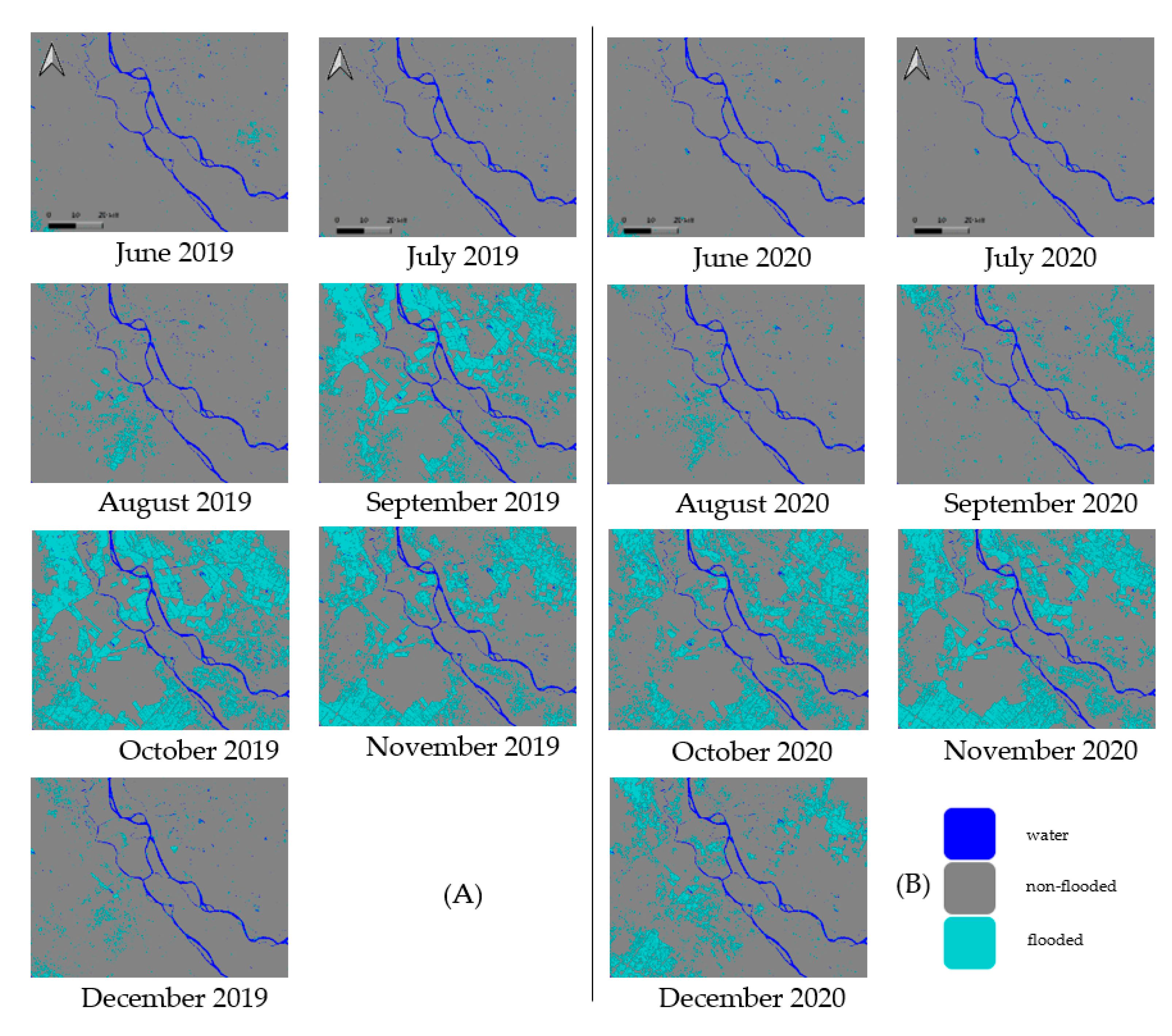
In this section, we present the results of mapping of the flooded and non-flooded areas of the studied zone using multi-date-based SAR techniques, Sentinel-1 dual-polarity (VV/VH). Time series inundation maps were generated from five images for each month of the wet season (6–7 months) by applying the CNN model (Figure 9).

The floodwater class was well highlighted over the entire inundated area as a result of applying the CNN algorithm during the wet season (Figure 9). A pixel-based spatial analysis is performed to determine the surface areas in km2 that was delineated with the CNN maps, in correlation with the precipitation data (Figure 9). It is noted that there is a good correlation between the precipitation and the flooded area superficies where the low precipitation that occurred during the period of March to July does not lead to an increase in flooded areas superficies. In 2019, the months in which the extension of the flooded area is the highest were September, October and November, reaching the maximum in October, while in 2020, there was a shift of one month, and thus the highest extension of flooded area is observed in October, November and December, reaching the maximum in November (Figure 10). It is interesting to note that the month with the least extension of flooded areas for both years was July, even though there was considerable precipitation. This precipitation occurred at the end of the month and its effects were observed in August.

3.3.2. Flood Mapping, Main Land Use/Land Cover (LULC)

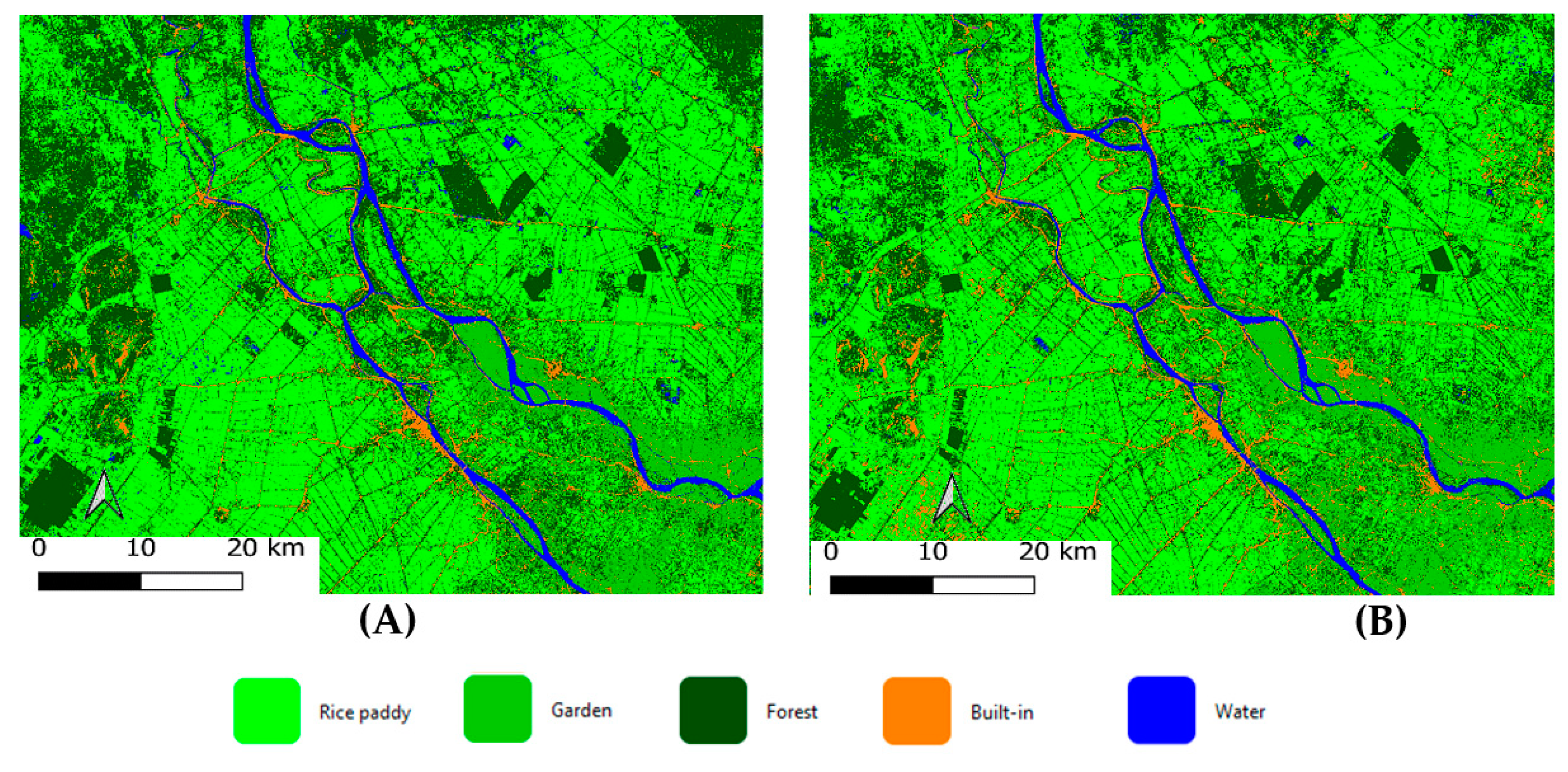
From the information on the maximum extension of the flooded areas (part of the floodable zones) for the two years (October 2019 and November 2020; Figure 10) the analysis first focused on the land use/land cover (LULC) classes before the wet season (Figure 10) to determine which land use classes were subsequently flooded. Analysis was then performed on the non-flooded LULC classes (Figure 11).

Figure 10 presents the spatial repartition of the LULC classes before the wet season in the study area. The CNN models have detected the five main classes, i.e., rice paddies, built-up areas, water, garden, and forests, for the years 2019 (Figure 11A) and 2020 (Figure 11B). Moreover,

Table 8. Area of land use/land cover before the wet season in 2019 and 2020.

	2019		2020
Class	Area (km2)	Percentage	Area (km2)	Percentage
Water	260.36	2%	318.92	3%
Rice paddy	5941.38	53%	6060.63	55%
Built-up	690.80	6%	426.14	4%
Garden	1605.34	15%	1272.24	11%
Forest	2605.34	24%	3035.02	27%

shows the superficies (km²) that covers each of these classes.

The spatial analysis of the LULC map shows that the built-up areas, rivers/wetlands and rice paddies were prominent and clear in the outputs of CNN. In both 2019 and 2020, rice fields occupied more than half of the study area (53% in 2019 and 55% in 2020) followed by forests (24% in 2019 and 27% in 2020) and gardens, which made up 15% and 11% of the landscape, respectively. The built-up area occupied 6% in 2019 and 4% in 2020. Water represented 2–3% of the landscape, while forests tended to be concentrated in the wetlands of the study area (Table 8).

By comparing the flood extents of the flood events (

Table 9. Area estimation of land use/land class impacted by flooding.

	2019		2020
Class	Area (km2)	Percentage	Area (km2)	Percentage
Water	25.42	1%	30.05	1%
Rice paddies	2615.26	58%	2075.67	53%
Built-up	409.66	9%	556.60	14%
Garden	1208.07	27%	1133.96	29%
Forest	220.56	5%	127.07	3%
Total of floodable area	4478.99		3923.37

), it was found that the 2020 flooded areas were smaller (3923.3 km²) than the 2019 flooded areas (4478.9 km²).

Although the rice paddies superficies were smaller, in 2019 the superficies of rice paddies impacted by flooding were greater than in 2020. Indeed, more than half of the rice fields were flooded both years: 58% in 2019 and 53% in 2020 (Figure 12). The flooding in both years significantly impacted another land use class with significant local economic value, gardens: 27% in 2019 and 29% in 2020. Urban areas were impacted much more strongly in 2020 (14%) than in 2019 (9%). In contrast, forests were less strongly impacted in 2020 than in 2019.

4. Discussion

The most frequent flooding in the Mekong Delta is mainly induced by the Mekong River flooding regime as well as by the surface flow. The construction of dyke systems from the early 1990s onwards to protect fields from flooding allows for third crop cultivation in some parts of the delta. However, this is not the case everywhere in our study area. Another category of floods is those caused by the distribution of a dense network of canals and controlled by dikes and lock gates. In this case flood monitoring is a hard task and relies mainly on data from a few meteorological stations in the region and on the hydrological models. However, flood forecasting from these models is becoming more difficult due to anthropogenic factors, sea level rise and environmental and climate changes [70] This study aimed at providing an accurate method for flood prone mapping in the Mekong Delta using satellite data and ML algorithms.

By testing the accuracy of the ML algorithm, the first objective of this study were to define an effective and validated method for detecting flooded and non-flooded areas in the Mekong Delta. This type of study could provide a large panel of users with the possibility and choice to reproduce the exact method in an automatic and standard way, which should allow the updating of a possible database shared between local institutes in an efficient way [71]. Thus, it was important not only use software algorithms and data that provide a reliable and accurate result but also that are available and reproducible, in order that the mapping can also be undertaken by the partners in Vietnam or in other concerned study areas. Regarding the data, we noticed that, although Sentinel-1 SAR data are widely used for flood monitoring due to their high spatial and temporal resolution and free availability, very few studies using Sentinel-1 SAR data for flood mapping and monitoring have been conducted in the Mekong Delta. For the algorithm choice, we have provided detailed results and the accuracy of three ML algorithms for image classification, via a comparative study. In addition, supervised and unsupervised classification methods have been widely applied for surface water mapping using satellite images [72] and have compared supervised and unsupervised machine learning methods, revealing an overall accuracy of the unsupervised water classification method of 89.3% [73], while in the present study, the accuracy has achieved higher values (globally higher than 95%). Although the supervised classification method is able to map water bodies efficiently, it could be a tedious task because of the creation of the training and the validation dataset, which could be time-consuming.

The flood maps derived from the algorithms tested here in our work were validated by overlaying them with metrological and hydrographical data. We noticed that the accuracy of the image classifications varies with the methods and techniques employed. Few studies have reported minor to moderate fluctuation in the accuracy of classification of flooded and non-flooded areas using different classifiers. Therefore, we attempt to pay a particular and detailed attention to the accuracy assessment and validation of the classification and mapping model, by comparing the results of the CNN model with other robust models such as MLP and RF. We noted that all models have the same trends of the accuracy indicators values. In general the accuracy indicators values achieved the highest values for months with maximum extension of flooded areas (October and then November) and the lowest values for months with less extension of flooded areas (July). However, the CNN model performed the best, achieving the highest accuracy. This accuracy analysis could be one of the added values of this study as it gives an idea of the performance of each model used and allows users to choose the appropriate one for flood and LULC mapping.

The Flood and Floodable Area Forecasting Model

In the field of flood mapping, the main objective is to distinguish between flooded and non-flooded areas, which can be treated as a binary classification process in which regions are labelled as “flood” or “non-flood.” In this study, the CNN classifier showed a very high overall accuracy of about 99% for flooded and non-flooded areas. It was directly used for binary classification in order to identify the regional floodable and non-floodable areas. In order to provide a simplified and reproducible approach, a 2D-CNN architecture was used for the generalized classification process.

Furthermore, we focused our analysis on the most flood-impacted zones of the study area (Table 9). It was found that the 2020 flooded areas were smaller (3923.3 km²) than the 2019 flooded areas (4478.9 km²). These differences in the extent of flooding could indicate that the flooded area should be analyzed in relation to the maximum level of the Mekong River. This level was recorded at Tan Chau station, and in 2019 it was almost 4 m compared to the level recorded in 2020 of less than 3 m. At the same time, the uncertainties of mapping using SAR techniques could be considered. It should be mentioned that the SAR signal may be influenced by speckle and thus by under- or over-detection of the flood extent, especially in urban and vegetated areas. In this context, the CNN framework aims to reduce classification errors associated with land cover heterogeneities and underlying complexity. This framework can efficiently distinguish permanent water from flood water even though minor misclassification errors may be observed among land cover classes.

In order to interpret and understand the driving forces behind the onset and progression of flooding in the Mekong Delta, it is important to understand the climate and hydrological regime in this extremely complex flooding environment. The most frequent flooding in the 203 delta is mainly induced by the Mekong River flooding regime as well as by the surface flow. The construction of dyke systems from the early 1990s onwards to protect fields from flooding allows for third crop cultivation in some parts of the delta. However, this is not the case everywhere in our study area. Another category of floods consists of those caused by the distribution of a dense network of canals and controlled by dikes and lock gates. We can admit that the flooding in the Mekong Delta has a series of secondary undesired and desired effects. The undesired effects of flooding lead to the destruction of infrastructure and crops. Meanwhile, floodwaters fertilize floodplain soils and can provide a habitat for aquatic animals, and when controlled, they enable irrigation activities and even energy generation. Based on the SAR time series alone, it is not possible to fully differentiate between the individual components, nor is it possible to distinguish between a “desirable flood” and an “undesirable flood’’ [26]. It is not always possible to distinguish between natural and man-made floods. However, interpretation can be more reliable in this respect if auxiliary data such as information on the type of land use and humane activities are available.

5. Conclusions

Floods are a recurrent risk in the Vietnamese Mekong Delta. This phenomenon is happening more frequently and with higher intensity due to climate change [74,75]. Indeed, the analysis and monitoring of flood events through mapping of flooded and floodable areas is becoming a priority in risk management. This study provides a systemic approach by exploring the potentials of advanced ML models with an optimal architectural design for flood and flood-prone area mapping from SAR images in tropical deltaic environments. In order to exploit the multi-temporal series of the Sentinel-1 images in dual polarization (VV and VH), a backscatter coefficient analysis was performed using a large amount of reference images (60 images per year and 5 images per month). Moreover, the hydrological regime data, the calendar of flooding and the rice cultivation period were incorporated in order to allow a much more reliable and accurate detection of changes during floods.

Three robust models of ML, namely CNN, MLP and RF, were developed, revealing high potentials for flood and floodable area mapping in the Mekong Delta. A comparative detailed analysis between different accuracy indicators recorded by the three ML models, with the correlation of flooding periods, could be considered especially important to allow for a perfect accuracy assessment. It was noted that the proposed CNN model demonstrated the highest reliability and flexibility for flood and floodable area mapping. These prediction results provide new insights into the patterns of flood variation in space and time in the Mekong Delta. Furthermore, the use of segmentation parameters adapted to seasonal and annual variations and the adaptation of CNN models to these variations are one of the original aspects of our classification method.

According to the results of the flood extent mapping derived from the application of the three ML algorithms, the predictions of the spatiotemporal flood forecast models based on the Sentinel-1 time series appear to be globally consistent. Furthermore, from a qualitative point of view, the magnitude of seasonal and inter-annual variations in flood extent was also consistent with significant peaks during the wet season and troughs during the dry season highlighted by the hydro-meteorological data. Indeed, peaks and troughs in flood extent are generally well aligned with the CNN mapping of flood events and floodable areas.

Although rice fields were the economic issue addressed in this study, a LULC analysis was also conducted to quantify the impact of flood risk on different land use classes with significant local economic value. This research suggests that the CNN model developed here could be generalized to other deltaic areas for future studies, using other types of remotely sensed images.

References

1. Kundzewicz, Z.W.; Kanae, S.; Seneviratne, S.; Handmer, J.; Nicholls, N.; Peduzzi, P.; Mechler, R.; Bouwer, L.; Arnell, N.; Mach, K.; et al. Flood Risk andzhong Climate Change–Global and Regional Perspectives. Hydrol. Sci. J. 2014, 59, 2014. [Google Scholar] [CrossRef]
2. Ahamed, A.; Bolten, J.; Doyle, C.; Fayne, J. Near Real-Time Flood Monitoring and Impact Assessment Systems. In Remote Sensing of Hydrological Extremes; Springer: Berlin/Heidelberg, Germany, 2017. [Google Scholar]
3. Dang, A.T.N.; Kumar, L. Application of Remote Sensing and GIS-Based Hydrological Modelling for Flood Risk Analysis: A Case Study of District 8, Ho Chi Minh City, Vietnam. Geomat. Nat. Hazards Risk 2017, 8, 1792–1811. [Google Scholar] [CrossRef]
4. Mojaddadi, H.; Pradhan, B.; Nampak, H.; Ahmad, N.; Ghazali, A.H. bin Ensemble Machine-Learning-Based Geospatial Approach for Flood Risk Assessment Using Multi-Sensor Remote-Sensing Data and GIS. Geomat. Nat. Hazards Risk 2017, 8, 1080–1102. [Google Scholar] [CrossRef]
5. Kontgis, C.; Schneider, A.; Ozdogan, M. Mapping Rice Paddy Extent and Intensification in the Vietnamese Mekong River Delta with Dense Time Stacks of Landsat Data. Remote Sens. Environ. 2015, 169, 255–269. [Google Scholar] [CrossRef]
6. Son, T.N.; Chen, C.-F.; Chen, C.-R.; Duc, H.-N.; Chang, L.-Y. A Phenology-Based Classification of Time-Series MODIS Data for Rice Crop Monitoring in Mekong Delta, Vietnam. Remote Sens. 2013, 6, 135–156. [Google Scholar] [CrossRef]
7. Karila, K.; Nevalainen, O.; Krooks, A.; Karjalainen, M.; Kaasalainen, S. Monitoring Changes in Rice Cultivated Area from SAR and Optical Satellite Images in Ben Tre and Tra Vinh Provinces in Mekong Delta, Vietnam. Remote Sens. 2014, 6, 4090–4108. [Google Scholar] [CrossRef]
8. Nguyen, T.T.H.; Bie, C.A.J.M.D.; Ali, A.; Smaling, E.M.A.; Chu, T.H. Mapping the Irrigated Rice Cropping Patterns of the Mekong Delta, Vietnam, through Hyper-Temporal SPOT NDVI Image Analysis. Int. J. Remote Sens. 2012, 33, 415–434. [Google Scholar] [CrossRef]
9. Kontgis, C.; Warren, M.S.; Skillman, S.W.; Chartrand, R.; Moody, D.I. Leveraging Sentinel-1 Time-Series Data for Mapping Agricultural Land Cover and Land Use in the Tropics. In Proceedings of the 2017 9th International Workshop on the Analysis of Multitemporal Remote Sensing Images (MultiTemp), Brugge, Belgium, 27–29 June 2017; pp. 1–4. [Google Scholar]
10. Martini, J.; Petzoldt, J.; Einsle, F.; Beesdo-Baum, K.; Höfler, M.; Wittchen, H.-U. Risk Factors and Course Patterns of Anxiety and Depressive Disorders during Pregnancy and after Delivery: A Prospective-Longitudinal Study. J. Affect Disord. 2015, 175, 385–395. [Google Scholar] [CrossRef]
11. Matgen, P.; Hostache, R.; Schumann, G.; Pfister, L.; Hoffmann, L.; Savenije, H.H.G. Towards an Automated SAR-Based Flood Monitoring System: Lessons Learned from Two Case Studies. Phys. Chem. Earth Parts A/B/C 2011, 36, 241–252. [Google Scholar] [CrossRef]
12. Twele, A.; Cao, W.; Plank, S.; Martinis, S. Sentinel-1-Based Flood Mapping: A Fully Automated Processing Chain. Int. J. Remote Sens. 2016, 37, 2990–3004. [Google Scholar] [CrossRef]
13. Amitrano, C.C.; Tregua, M.; Russo Spena, T.; Bifulco, F. On Technology in Innovation Systems and Innovation-Ecosystem Perspectives: A Cross-Linking Analysis. Sustainability 2018, 10, 3744. [Google Scholar] [CrossRef]
14. Bioresita, F.; Puissant, A.; Stumpf, A.; Malet, J.-P. A Method for Automatic and Rapid Mapping of Water Surfaces from Sentinel-1 Imagery. Remote Sens. 2018, 10, 217. [Google Scholar] [CrossRef]
15. Carreño Conde, F.; De Mata Muñoz, M. Flood Monitoring Based on the Study of Sentinel-1 SAR Images: The Ebro River Case Study. Water 2019, 11, 2454. [Google Scholar] [CrossRef]
16. Martinis, S.; Plank, S.; Ćwik, K. The Use of Sentinel-1 Time-Series Data to Improve Flood Monitoring in Arid Areas. Remote Sens. 2018, 10, 583. [Google Scholar] [CrossRef]
17. Zhang, M.; Chen, F.; Liang, D.; Tian, B.; Yang, A. Use of Sentinel-1 GRD SAR Images to Delineate Flood Extent in Pakistan. Sustainability 2020, 12, 5784. [Google Scholar] [CrossRef]
18. Jung, H.C.; Hamski, J.; Durand, M.; Alsdorf, D.; Hossain, F.; Lee, H.; Hossain, A.K.M.A.; Hasan, K.; Khan, A.S.; Hoque, A.K.M.Z. Characterization of Complex Fluvial Systems Using Remote Sensing of Spatial and Temporal Water Level Variations in the Amazon, Congo, and Brahmaputra Rivers. Earth Surf. Process. Landforms 2010, 35, 294–304. [Google Scholar] [CrossRef]
19. Schlaffer, S.; Matgen, P.; Hollaus, M.; Wagner, W. Flood Detection from Multi-Temporal SAR Data Using Harmonic Analysis and Change Detection. Int. J. Appl. Earth Observat. Geoinformat. 2015, 38, 15–24. [Google Scholar] [CrossRef]
20. Alsdorf, D.; Bates, P.; Melack, J.; Wilson, M.; Dunne, T. Spatial and Temporal Complexity of the Amazon Flood Measured from Space. Geophys. Res. Lett. 2007, 34, L08402. [Google Scholar] [CrossRef]
21. Wilusz, D.C.; Zaitchik, B.F.; Anderson, M.C.; Hain, C.R.; Yilmaz, M.T.; Mladenova, I.E. Monthly Flooded Area Classification Using Low Resolution SAR Imagery in the Sudd Wetland from 2007 to 2011. Remote Sens. Environ. 2017, 194, 205–218. [Google Scholar] [CrossRef]
22. Bouvet, A.; Le Toan, T. Use of ENVISAT/ASAR Wide-Swath Data for Timely Rice Fields Mapping in the Mekong River Delta. Remote Sens. Environ. 2011, 115, 1090–1101. [Google Scholar] [CrossRef]
23. Cao, H.; Zhang, H.; Wang, C.; Zhang, B. Operational Flood Detection Using Sentinel-1 SAR Data over Large Areas. Water 2019, 11, 786. [Google Scholar] [CrossRef]
24. Chini, M.; Hostache, R.; Giustarini, L.; Matgen, P. A Hierarchical Split-Based Approach for Parametric Thresholding of SAR Images: Flood Inundation as a Test Case. IEEE Transact. Geosci. Remote Sens. 2017, 55, 6975–6988. [Google Scholar] [CrossRef]
25. Greifeneder, F.; Wagner, W.; Sabel, D.; Naeimi, V. Suitability of SAR Imagery for Automatic Flood Mapping in the Lower Mekong Basin. Int. J. Remote Sens. 2014, 35, 2857–2874. [Google Scholar] [CrossRef]
26. Kuenzer, C.; Guo, H.; Huth, J.; Leinenkugel, P.; Li, X.; Dech, S. Flood Mapping and Flood Dynamics of the Mekong Delta: ENVISAT-ASAR-WSM Based Time Series Analyses. Remote Sens. 2013, 5, 687–715. [Google Scholar] [CrossRef]
27. Niculescu, S.; Lardeux, C.; Hanganu, J.; Mercier, G.; David, L. Change Detection in Floodable Areas of the Danube Delta Using Radar Images. Nat. Hazards 2015, 78, 1899–1916. [Google Scholar] [CrossRef]
28. Niculescu, S.; Lardeux, C.; Guttler, F.; Rudant, J.-P. Multisensor Systems and Flood Risk Management. Application to the Danube Delta Using Radar and Hyperspectral Imagery. Teledetection 2010, 9, 271–288. [Google Scholar]
29. Niculescu, S.; Lardeux, C.; Frison, P.-L.; Rudant, J.-P. L’approche Sociale et Radar de la Gestion du Risque d’inondation dans le Delta du Danube. Houille Blanche 2009, 95, 81–87. [Google Scholar] [CrossRef]
30. Pulvirenti, L.; Chini, M.; Pierdicca, N.; Boni, G. Use of SAR Data for Detecting Floodwater in Urban and Agricultural Areas: The Role of the Interferometric Coherence. IEEE Transact. Geosci. Remote Sens. 2016, 54, 1532–1544. [Google Scholar] [CrossRef]
31. Schumann, G.; Bates, P.D.; Horritt, M.S.; Matgen, P.; Pappenberger, F. Progress in Integration of Remote Sensing–Derived Flood Extent and Stage Data and Hydraulic Models. Rev. Geophys. 2009, 47, RG4001. [Google Scholar] [CrossRef]
32. Laugier, O.; Fellah, K.; Tholey, N.; Meyer, C.; Fraipont, P. High Temporal Detection and Monitoring of Flood Zone Dynamic Using ERS Data around Catastrophic Narural Events: The 1993 and 1994 Camargue Flood Events. Flood Detection Using ERS-1 SAR Data 1997. In Proceedings of the Space at the Service of Our Environment, Florence, Italy, 14–21 March 1997. [Google Scholar]
33. Martinis, S.; Rieke, C. Backscatter Analysis Using Multi-Temporal and Multi-Frequency SAR Data in the Context of Flood Mapping at River Saale, Germany. Remote Sens. 2015, 7, 7732–7752. [Google Scholar] [CrossRef]
34. Camps-Valls, G.; Tuia, D.; Zhu, X.X.; Reichstein, M. Deep Learning for the Earth Sciences: A Comprehensive Approach to Remote Sensing, Climate Science and Geosciences, 1st ed; Wiley: Hoboken, NJ, USA, 2021; ISBN 978-1-119-64614-3. [Google Scholar]
35. Sun, A.Y.; Scanlon, B.R. How Can Big Data and Machine Learning Benefit Environment and Water Management: A Survey of Methods, Applications, and Future Directions. Environ. Res. Lett. 2019, 14, 073001. [Google Scholar] [CrossRef]
36. Tahmasebi, P.; Kamrava, S.; Bai, T.; Sahimi, M. Machine Learning in Geo- and Environmental Sciences: From Small to Large Scale. Adv. Water Resour. 2020, 142, 103619. [Google Scholar] [CrossRef]
37. Zhong, S.; Zhang, K.; Bagheri, M.; Burken, J.G.; Gu, A.; Li, B.; Ma, X.; Marrone, B.L.; Ren, Z.J.; Schrier, J.; et al. Machine Learning: New Ideas and Tools in Environmental Science and Engineering. Environ. Sci. Technol. 2021, 55, 12741–12754. [Google Scholar] [CrossRef]
38. Wagenaar, D.; Curran, A.; Balbi, M.; Bhardwaj, A.; Soden, R.; Hartato, E.; Mestav Sarica, G.; Ruangpan, L.; Molinario, G.; Lallemant, D. Invited Perspectives: How Machine Learning Will Change Flood Risk and Impact Assessment. Nat. Hazards Earth Syst. Sci. 2020, 20, 1149–1161. [Google Scholar] [CrossRef]
39. Chen, J.; Huang, G.; Chen, W. Towards Better Flood Risk Management: Assessing Flood Risk and Investigating the Potential Mechanism Based on Machine Learning Models. J. Environ. Manage. 2021, 293, 112810. [Google Scholar] [CrossRef]
40. Yang, T.; Sun, F.; Gentine, P.; Liu, W.; Wang, H.; Yin, J.; Du, M.; Liu, C. Evaluation and Machine Learning Improvement of Global Hydrological Model-Based Flood Simulations. Environ. Res. Lett. 2019, 14, 114027. [Google Scholar] [CrossRef]
41. Costache, R. Flood Susceptibility Assessment by Using Bivariate Statistics and Machine Learning Models—A Useful Tool for Flood Risk Management. Water Resour. Manage. 2019, 33, 3239–3256. [Google Scholar] [CrossRef]
42. Bui, D.T.; Ngo, P.-T.T.; Pham, T.D.; Jaafari, A.; Minh, N.Q.; Hoa, P.V.; Samui, P. A Novel Hybrid Approach Based on a Swarm Intelligence Optimized Extreme Learning Machine for Flash Flood Susceptibility Mapping. CATENA 2019, 179, 184–196. [Google Scholar] [CrossRef]
43. Singh, A.; Singh, P. Image Classification: A Survey. J. Inform. Electr. Elecrtonics Eng. 2020, 1, 1–9. [Google Scholar] [CrossRef]
44. Gašparović, M.; Klobučar, D. Mapping Floods in Lowland Forest Using Sentinel-1 and Sentinel-2 Data and an Object-Based Approach. Forests 2021, 12, 553. [Google Scholar] [CrossRef]
45. Bui, D.T.; Tsangaratos, P.; Nguyen, V.-T.; Liem, N.V.; Trinh, P.T. Comparing the Prediction Performance of a Deep Learning Neural Network Model with Conventional Machine Learning Models in Landslide Susceptibility Assessment. CATENA 2020, 188, 104426. [Google Scholar] [CrossRef]
46. Khan, S.; Yairi, T. A Review on the Application of Deep Learning in System Health Management. Mechan. Syst. Signal Process. 2018, 107, 241–265. [Google Scholar] [CrossRef]
47. Rawat, W.; Wang, Z. Deep Convolutional Neural Networks for Image Classification: A Comprehensive Review. Neural. Comput. 2017, 29, 2352–2449. [Google Scholar] [CrossRef] [PubMed]
48. Voulodimos, A.; Doulamis, N.; Doulamis, A.; Protopapadakis, E. Deep Learning for Computer Vision: A Brief Review. Comput. Intell. Neurosci. 2018, 2018, e7068349. [Google Scholar] [CrossRef]
49. Nemni, E.; Bullock, J.; Belabbes, S.; Bromley, L. Fully Convolutional Neural Network for Rapid Flood Segmentation in Synthetic Aperture Radar Imagery. Remote Sens. 2020, 12, 2532. [Google Scholar] [CrossRef]
50. Li, Y.; Martinis, S.; Wieland, M. Urban Flood Mapping with an Active Self-Learning Convolutional Neural Network Based on TerraSAR-X Intensity and Interferometric Coherence. ISPRS J. Photogramm. Remote Sens. 2019, 152, 178–191. [Google Scholar] [CrossRef]
51. Kang, W.; Xiang, Y.; Wang, F.; Wan, L.; You, H. Flood Detection in Gaofen-3 SAR Images via Fully Convolutional Networks. Sensors 2018, 18, 2915. [Google Scholar] [CrossRef]
52. Shen, X.; Anagnostou, E.N.; Allen, G.H.; Robert Brakenridge, G.; Kettner, A.J. Near-Real-Time Non-Obstructed Flood Inundation Mapping Using Synthetic Aperture Radar. Remote Sens. Environ. 2019, 221, 302–315. [Google Scholar] [CrossRef]
53. Phan, T.H. Suivi Des Surfaces Rizicoles Par Télédétection Radar. Ph.D. Thesis, Université de Toulouse, Toulouse, France, 2018; p. 3. [Google Scholar]
54. Phan, A.; Ha, D.N.; Man, C.D.; Nguyen, T.T.; Bui, H.Q.; Nguyen, T.T.N. Rapid Assessment of Flood Inundation and Damaged Rice Area in Red River Delta from Sentinel 1A Imagery. Remote Sens. 2019, 11, 2034. [Google Scholar] [CrossRef]
55. Drǎguţ, L.; Csillik, O.; Eisank, C.; Tiede, D. Automated Parameterisation for Multi-Scale Image Segmentation on Multiple Layers. ISPRS J. Photogramm. Remote Sens. 2014, 88, 119–127. [Google Scholar] [CrossRef]
56. Ryherd, S.; Woodcock, C. Combining Spectral and Texture Data in the Segmentation of Remotely Sensed Images. Photogramm. Eng. Remote Sens. 1996, 62, 181–194. [Google Scholar]
57. Baatz, M.; Schäpe, A. Multiresolution Segmentation: An Optimization Approach for High Quality Multi-Scale Image Segmentation. 2000. Available online: https://pdf4pro.com/cdn/multiresolution-segmentation-an-optimization-approach-5aca1e.pdf (accessed on 15 December 2022).
58. Liu, T.; Elmikaty, M.; Stathaki, T. SAM-RCNN: Scale-Aware Multi-Resolution Multi-Channel Pedestrian Detection. arXiv 2018, arXiv:1808.02246. [Google Scholar]
59. Goodfellow, I.; Bengio, Y.; Courville, A. Deep Learning; MIT Press: Cambridge, MA, USA, 2016. [Google Scholar]
60. LeCun, Y.; Boser, B.; Denker, J.S.; Henderson, D.; Howard, R.E.; Hubbard, W.; Jackel, L.D. Backpropagation Applied to Handwritten Zip Code Recognition. Neural Computat. 1989, 1, 541–551. [Google Scholar] [CrossRef]
61. Borovykh, A.; Bohte, S.; Oosterlee, C.W. Conditional Time Series Forecasting with Convolutional Neural Networks. arXiv 2018, arXiv:1703.04691. [Google Scholar]
62. Gebrehiwot, A.; Hashemi-Beni, L.; Thompson, G.; Kordjamshidi, P.; Langan, T.E. Deep Convolutional Neural Network for Flood Extent Mapping Using Unmanned Aerial Vehicles Data. Sensors 2019, 19, 1486. [Google Scholar] [CrossRef]
63. Breiman, L. Random Forests. Machine Learn. 2001, 45, 5–32. [Google Scholar] [CrossRef]
64. Balzter, H.; Cole, B.; Thiel, C.; Schmullius, C. Mapping CORINE Land Cover from Sentinel-1A SAR and SRTM Digital Elevation Model Data Using Random Forests. Remote Sens. 2015, 7, 14876–14898. [Google Scholar] [CrossRef]
65. Rüetschi, M.; Schaepman, M.E.; Small, D. Using Multitemporal Sentinel-1 C-Band Backscatter to Monitor Phenology and Classify Deciduous and Coniferous Forests in Northern Switzerland. Remote Sens. 2018, 10, 55. [Google Scholar] [CrossRef]
66. Ghazaryan, G.; Dubovyk, O.; Löw, F.; Lavreniuk, M.; Kolotii, A.; Schellberg, J.; Kussul, N. A Rule-Based Approach for Crop Identification Using Multi-Temporal and Multi-Sensor Phenological Metrics. Eur. J. Remote Sens. 2018, 51, 511–524. [Google Scholar] [CrossRef]
67. Olofsson, P.; Foody, G.M.; Herold, M.; Stehman, S.V.; Woodcock, C.E.; Wulder, M.A. Good Practices for Estimating Area and Assessing Accuracy of Land Change. Remote Sens. Environ. 2014, 148, 42–57. [Google Scholar] [CrossRef]
68. Niculescu, S.; Boissonnat, J.-B.; Lardeux, C.; Roberts, D.; Hanganu, J.; BILLEY, A.; Constantinescu, A.; Doroftei, M. Synergy of High-Resolution Radar and Optical Images Satellite for Identification and Mapping of Wetland Macrophytes on the Danube Delta. Remote Sens. 2020, 12, 2188. [Google Scholar] [CrossRef]
69. Stehman, S.; Foody, G. Key Issues in Rigorous Accuracy Assessment of Land Cover Products. Remote Sens. Environ. 2019, 231, 111199. [Google Scholar] [CrossRef]
70. Duc Tran, D.; van Halsema, G.; Hellegers, P.J.G.J.; Phi Hoang, L.; Quang Tran, T.; Kummu, M.; Ludwig, F. Assessing Impacts of Dike Construction on the Flood Dynamics of the Mekong Delta. Hydrol. Earth Syst. Sci. 2018, 22, 1875–1896. [Google Scholar] [CrossRef]
71. Bengoufa, S.; Niculescu, S.; Mihoubi, M.K.; Belkessa, R.; Ali, R.; Rabehi, W.; Abbad, K. Machine Learning and Shoreline Monitoring Using Optical Satellite Images: Case Study of the Mostaganem Shoreline, Algeria. J. Appl. Remote Sens. 2021, 15, 026509. [Google Scholar] [CrossRef]
72. Martinis, S.; Twele, A.; Voigt, S. Unsupervised Extraction of Flood-Induced Backscatter Changes in SAR Data Using Markov Image Modeling on Irregular Graphs. IEEE Trans. Geosci. Remote Sens. 2011, 49, 251–263. [Google Scholar] [CrossRef]
73. Bangira, T.; Alfieri, S.M.; Menenti, M.; van Niekerk, A. Comparing Thresholding with Machine Learning Classifiers for Mapping Complex Water. Remote Sens. 2019, 11, 1351. [Google Scholar] [CrossRef]
74. Hoang, L.P.; Biesbroek, R.; Tri, V.P.D.; Kummu, M.; van Vliet, M.T.H.; Leemans, R.; Kabat, P.; Ludwig, F. Managing Flood Risks in the Mekong Delta: How to Address Emerging Challenges under Climate Change and Socioeconomic Developments. Ambio 2018, 47, 635–649. [Google Scholar] [CrossRef]
75. Triet, N.V.K.; Dung, N.V.; Hoang, L.P.; Duy, N.L.; Tran, D.D.; Anh, T.T.; Kummu, M.; Merz, B.; Apel, H. Future Projections of Flood Dynamics in the Vietnamese Mekong Delta. Sci. Total Environ. 2020, 742, 140596. [Google Scholar] [CrossRef]
Figure 1. Location of the study site and weather and hydrological stations.
Remotesensing 15 02001 g001
Figure 2. Schematic representation of C band backscatter mechanisms for rice (Oryza sativa) with three main phases in Mekong Delta (vegetative phase, reproductive phase and ripening phase); (a) forward reflection (specular); (b) Double-bounce; and (c) volume scattering.
Remotesensing 15 02001 g002
Figure 3. Process flowchart for flood zones, permanent waters and land cover mapping: pre-processing (A), image processing (B) and post-classification (C).
Remotesensing 15 02001 g003
Figure 4. Generalized CNN classifier with the 2D-CNN architecture.
Remotesensing 15 02001 g004
Figure 5. The structure of a three-layer multi-layer perceptron neural network with three hidden nodes and five output classes. Each hidden layer is directly connected to each component of the input layer and also to each component in the output layer.
Remotesensing 15 02001 g005
Figure 6. MLP model accuracy curve with epoch = 200.
Remotesensing 15 02001 g006
Figure 7. (A) Daily rainfall and daily water levels of the Mekong River recorded at the Tan Chau hydro-meteorological station during 2020. Seasons of the three rice cycles (rice season winter-spring, summer-autumn and autumn-winter). Observations of SAR Sentinel-1: 60 images for 2020; (B) Temporal VH profiles of non-flooded rice paddies during the wet season and of flooded rice paddies during the wet season; (C) Temporal VV profiles of non-flooded rice paddies during the wet season and of flooded rice paddies during the wet season.
Remotesensing 15 02001 g007
Figure 8. (A) Daily rainfall and daily water levels of the Mekong River recorded at the Tan Chau hydro-meteorological station during 2019. Seasons of the three rice cycles (rice seasons winter-spring, summer-autumn and autumn-winter). SAR Sentinel-1 observations: 60 images for 2019; (B) temporal VH profiles of non-flooded rice paddies during the wet season and of flooded rice paddies during the wet season; (C) temporal VV profiles of non-flooded rice paddies during the wet season and of flooded rice paddies during the wet season.
Remotesensing 15 02001 g008
Figure 9. Flood mapping by CNN model: (A) Flooded areas in 2019; and (B) Flooded areas in 2020 by month in the wet season, from June to December.
Remotesensing 15 02001 g009
Figure 10. Average monthly rainfall; Maximum monthly water levels and flooded area in km2 for 2019 and 2020.
Remotesensing 15 02001 g010
Figure 11. Land use/land cover (LULC) before the wet season (A) 2019 and (B) 2020 by CNN classifier.
Remotesensing 15 02001 g011
Figure 12. Land use/land cover (LULC) during the wet season (A) 2019 and (B) 2020 by CNN classifier.
Remotesensing 15 02001 g012