Communication

Mapping Wheat Take-All Disease Levels from Airborne Hyperspectral Images Using Radiative Transfer Models

College of Information and Management Science, Henan Agricultural University, Zhengzhou 450002, China
*
Author to whom correspondence should be addressed.
Remote Sens. 2023, 15(8), 1960; https://doi.org/10.3390/rs15081960
Submission received: 31 January 2023 / Revised: 4 April 2023 / Accepted: 5 April 2023 / Published: 7 April 2023

Abstract

:
Take-all is a root disease that can severely reduce wheat yield, and wheat leaves with take-all disease show a large amount of chlorophyll loss. The PROSAIL model has been widely used for the inversion of vegetation physiological parameters with a clear physical meaning of the model and high simulation accuracy. Based on the chlorophyll deficiency characteristics, the reflectance data under different canopy chlorophyll contents were simulated using the PROSAIL model. In addition, inverse models of spectral reflectance profiles and canopy chlorophyll contents were constructed using a one-dimensional convolutional neural network (1D-CNN), and a transfer learning approach was used to detect the take-all disease levels. The spectral reflectance data of winter wheat acquired by an airborne imaging spectrometer during the filling period were used as input parameters of the model to obtain the chlorophyll content of the canopy. Finally, the results of the distribution of winter wheat take-all disease were mapped based on the relationship between take-all disease and the chlorophyll content of the canopy. The results showed that classification based on the deep learning model performed well for winter wheat take-all monitoring. This study can provide some reference basis for high-precision winter wheat take-all disease monitoring and can also provide some technical method references and ideas for remote sensing crop pest and disease remote sensing mapping.

1. Introduction

Take-all, which is caused by Gaeumannomyces graminis var tritici, is a soil-borne root disease of wheat that has spread worldwide [1,2]. Take-all can affect wheat throughout its reproductive stage and is highly destructive. The occurrence of take-all disease can have a large impact on wheat yield, ranging from 10% yield loss to more than 50% loss or even crop failure. Effective control of wheat take-all is essential to ensure the level of wheat production and to improve farmers’ economic income [3].
Hyperspectral images, which can obtain continuous and fine spectral curves at any point in space, have become an important tool for the study of wheat disease [4,5,6,7]. In recent years, several studies have been conducted using UAV hyperspectral images for wheat take-all disease [8,9]. In these studies, the spectral features of wheat take-all were extracted from hyperspectral images, and statistical methods or machine learning methods were used to build regression models between vegetation indices and take-all. Finally, the classification results of take-all were obtained. In the above-mentioned methods, the characteristic bands of take-all must be found, and the best spectral indices in the detection process must be selected. Feature selection is the process of selecting the most relevant spectral bands from raw high-dimensional spectral data for subsequent analysis or modeling. By selecting the optimal spectral bands, feature selection can significantly reduce the computational cost of processing high spectral data, while reducing the impact of noise interference by eliminating spectral bands that have no contribution to the target variable, simplifying the modeling process, and improving model accuracy. However, feature selection cannot fully reflect all the information in the original spectral data, resulting in information loss. Additionally, it may not accurately capture all the features in the original spectral data, thereby introducing bias. Domain knowledge and experience are also required when selecting spectral bands. In addition to the obvious changes in spectral characteristics, the chlorophyll content of wheat canopies affected by take-all disease was also significantly reduced compared to that of normal leaves.
Therefore, using a vegetation radiative transfer model to invert canopy chlorophyll content can be used to determine the severity of take-all disease based on the deviation of chlorophyll content from normal values. Vegetation radiative transfer models are mathematical models based on radiation transfer theory that describes the interaction between vegetation and radiation. Common vegetation radiative transfer models include PROSAIL, PROSPECT, SAIL, and 4SAIL. PROSAIL is a flexible, accurate, and easy-to-use vegetation radiative transfer model that can simulate spectral reflectance and radiative transfer for various vegetation types. PROSAIL considers the impact of vegetation structure on radiative transfer and accurately models spectral reflectance and radiative transfer. In addition, PROSAIL can also consider the effects of changes in vegetation parameters on radiative transfer, such as chlorophyll content and coverage. PROSAIL has proven to be one of the most successful canopy radiative transfer models for crops, and high accuracy can be obtained in canopy chlorophyll inversion using PROSAIL [10,11,12,13,14,15,16,17,18,19].
In recent years, with the rapid development of deep learning, convolutional neural networks (CNNs) have been used to reduce model complexity with sparse connections and weight sharing and have unique advantages in extracting data features. CNNs have been widely used in remote sensing image target recognition, feature classification, etc. [20,21,22,23,24,25,26,27,28,29]. When using deep learning models for ground parameter inversion, to obtain a high-quality inversion model, a large amount of sample data is required to train the model. In addition, the acquisition of ground measurement parameters is generally time-consuming, and it is difficult to obtain a large amount of high-quality sample data. Therefore, we consider using the PROSAIL physical model to generate training samples. Transfer learning is a machine learning method that leverages the similarity between data, tasks, or models to apply a pre-trained model from a source domain to a new target domain. We first pre-train the model with a large simulated dataset so that the network model learns the basic feature information of the canopy spectrum; then, we use a relatively small number of measured datasets to transfer the pre-trained model using feature extraction methods to obtain more realistic prediction results.
Based on the above issues, we explored the use of canopy spectral features for chlorophyll content inversion and established an algorithm to discriminate wheat take-all disease classes based on the chlorophyll content. For winter wheat at the filling stage, canopy reflectance profiles with different chlorophyll contents were constructed using the PROSAIL model. A pre-trained model was obtained using the simulated reflectance curve as the input data and the canopy chlorophyll content as the output result. Then, the model parameters were fine-tuned based on the ground survey data, while the relationship between chlorophyll content and wheat take-all disease was determined based on the ground survey data. Finally, the spatial distribution results of the disease indices of winter wheat take-all were obtained using the hyperspectral UAV data.

2. Materials and Methods

2.1. Study Area

The study area was located in Pei Cheng, Luohe City, Henan Province (33°43 N, 113°50 E), and the wheat sowing date in the study area was 12 October 2016. The management during the growth stage was the same as that of a high-yielding field, and the location distribution of the study area is shown in Figure 1. Hyperspectral data were collected from 11:00–13:00 on 21 May 2017, when the winter wheat was in the filling stage. To support the flight experiment, a ground data survey was conducted simultaneously, and 20 sample areas (Figure 1C) were selected in the test area for chlorophyll measurement and allograft disease survey, each with an area of 1 m 2 .
When obtaining ground data for wheat, canopy reflectance was measured using an Analytical Spectral Devices (ASD) spectrometer, ASD FieldSpec HandHeld is a lightweight, reliable, and high-resolution portable spectrometer for in-field hyperspectral analysis. It measures the spectral reflectance of samples in the range 350–2500 nm and is widely used in agriculture, geology, environmental monitoring, and other fields. Representative wheat plants were destructively obtained from each sample area and brought back to the laboratory. Chlorophyll was extracted using 95% ethanol and the chlorophyll content was determined by using the colorimetric method, at which time the chlorophyll content was calculated in mgg, i.e., the mass of chlorophyll contained in a unit mass of leaves. For consistency in terms of the chlorophyll units obtained from remote sensing images, the chlorophyll concentration units were converted to μ g/cm 2 , the mass of chlorophyll per unit leaf area, using the specific leaf weight of the leaves.

2.2. Experimental Dataset

In the flight test, the UHD185 airborne high-speed imaging spectrometer was used. This spectrometer can be used to obtain full-frame, nonscanning, real-time imaging, has a spectral range of 450–950 nm, a spectral resolution of 4 nm, and a total of 125 spectral channels. The UAV route height is 50 m, the heading overlap is 80%, and the side overlap is 60%. The UHD185 airborne high-speed imaging spectrometer acquires the data mainly consisting of hyperspectral cube images as well as panchromatic JPG images. The pre-processing of the UHD185 hyperspectral images mainly includes three parts: image stitching, image registration, and extraction of the average spectrum of the corn canopy in the experimental area. The pre-processing flow of the high-spectral image in this study is as follows: (1) Use Cube-Pilot software to fuse grayscale images and high-spectral images; (2) Use Agisoft PhotoScan software to stitch the obtained images; (3) Based on ground feature points, perform geometric correction on the images; (4) Crop and generate high-spectral images in the study area. Considering that hyperspectral data are susceptible to noise during acquisition and transmission, and may have problems related to baseline translation and drift, causing distortion of spectral features, Savitzky–Golay [30] (SG) filtering was chosen for noise removal and the smoothing of reflectance curves.
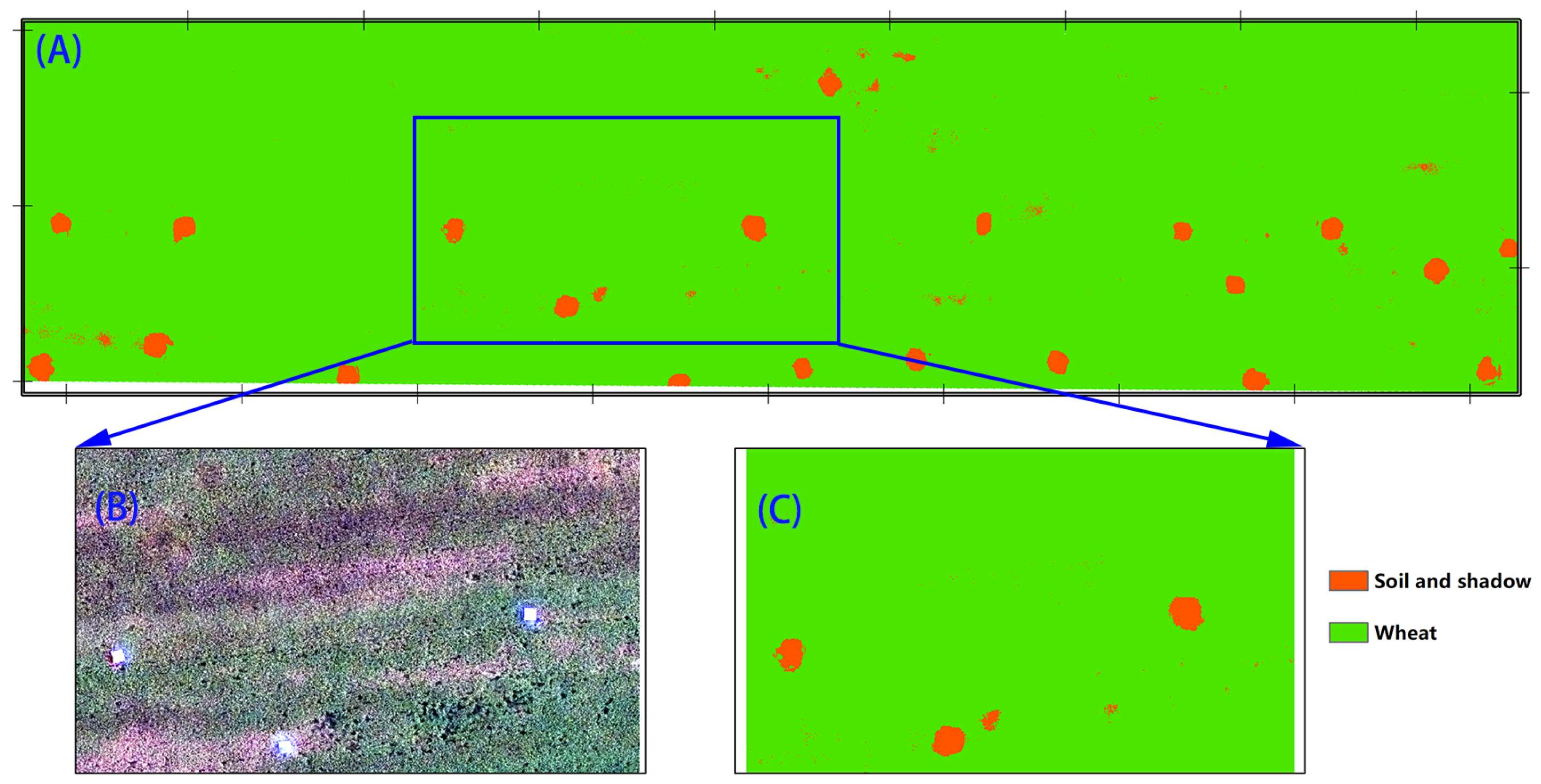
For the acquired hyperspectral images, the land types were labeled manually for training samples, and a support vector machine [31] (SVM) was used for land cover classification to distinguish winter wheat from weeds and background soil. A binary mask was eventually generated to exclude weed and background soil pixels from the UAV images (Figure 2) for further processing.
The chlorophyll content of winter wheat with take-all disease was reduced to varying degrees relative to normal growth, and the more severe the take-all disease was, the lower the chlorophyll content. Combining the ground survey data with expert experience, the threshold relationship between the levels of take-all disease and chlorophyll content can be determined using Table 1.

2.3. PROSAIL Model

The PROSAIL [32,33] model is composed of two sub-models, PROSPECT-D [34,35] and 4SAIL [36,37], capable of calculating the hemispherical reflectance and transmittance of leaves within a wavelength range of 400 nm to 2500 nm (1 nm increments). PROSPECT-D is a leaf radiative transfer model developed from the flat plate model, which assumes that leaves are stacked by N homogeneous layers separated by N − 1 layers of air. The PROSPECT-D model has seven input parameters, namely, leaf structural parameters, chlorophyll content, carotenoid content, brown pigment content, equivalent water thickness, dry matter content, and anthocyannins. The SAIL model is a bidirectional reflectance model for the vegetation canopy that assumes a continuous, horizontally uniform vegetation canopy and uses leaf reflectance and transmittance as input parameters to simulate the spectral and directional reflectance of plant canopies at any solar incidence angle and observation direction. The input parameters of the SAIL model mainly include the leaf area index, mean leaf inclination, hot spot, soil reflectance, and geometric parameters.
The SAIL model is a two-way reflectance model for the vegetation canopy, which assumes a continuous, horizontally homogeneous vegetation canopy with leaf reflectance. The input parameters of the 4SAIL model include leaf area index, mean leaf inclination, hot spots, soil reflectance, and geometric parameters. To construct the simulation data required for the inversion of the canopy chlorophyll content and combine the sensitivity of each parameter in the PROSAIL model to the canopy reflectance of the simulation results [38], the simulation parameters were set as shown in Table 2. For the two variable parameters, chlorophyll (C a b ) and leaf area index (LAI), in the generated simulation data, C a b varied from 10 to 80, and the step size was set to 1. The LAI, as another important parameter, varied from 1 to 8, and the step size was 0.1. The remaining parameters were set to fixed values or default values, among which the number of leaf layers N, which is related to the leaf structure, could not be measured directly. In this paper, only the winter wheat leaves during the filling period were considered, so the value of N was set to 1.5 [39]. The carotenoid content C a r was set to a fixed value of 6 μ g/cm 2 [40]. C w is mainly affected by the spectrum after 1000 nm in the NIR band and was set to a fixed value of 0.01 cm. The dry matter concentration C m has a certain effect on the visible NIR spectrum of the canopy, but the effect is weak, a fixed value of 0.005 μ g/cm 2 was set for C m . Parameters LIDFa and LIDFb control the average leaf slope and the distribution bimodality, respectively. We set the LIDFa and LIDFb of winter wheat to spherical [41] (LIDFa = 0.35 LIDFb = 0.15 ) according to the literature. The soil reflectance (Psoil) was assumed to be Lambertian in this study. For wheat leaves at the filling stage, the canopy was set as horizontal, and the hot spot parameter was 0.01. The angle parameter was set as the local solar incidence angle at 12:00 noon, the observed zenith angle was 0°, and the relative azimuth angle was 90°.
The canopy spectral reflectance interval output by the PROSAIL model was 1 nm, while the spectral resolution of the UAV hyperspectral data was 4 nm. The spectra in the simulated data were sampled using the mean value to make the spectral interval consistent with the 4 nm of the hyperspectral data, which is convenient for the subsequent comparison between the data.

2.4. CNN and Transfer Learning

CNN is a deep feedforward neural network with local connectivity and weight sharing. The CNN generally consists of cross-stacked convolutional, convergence, and fully connected layers. The fully-connected layer is generally the top layer of the convolutional network. CNN has three structural properties: local connectivity, weight sharing, and convergence. These features make the CNN invariant in translation, scaling, and rotation operations to a certain extent. CNN is mainly used in various image and video analysis tasks (e.g., image classification, object recognition, and image segmentation), and the accuracy of a CNN is generally far beyond that of other neural network models.
The structure of the 1D-CNN model for winter wheat take-all disease discrimination was designed with sixteen layers: an input layer, four CNN layers, pooling and dropout layers, two dense layers, and an output layer. When constructing the model, each piece of data was transformed into the appropriate form. The input layer was fed with reflectance profiles of hyperspectral data, followed by adaptive feature extraction and data dimensionality compression by the 1D-CNN and pooling layers, respectively, and the output layer is a fully connected layer with a softmax activation function.
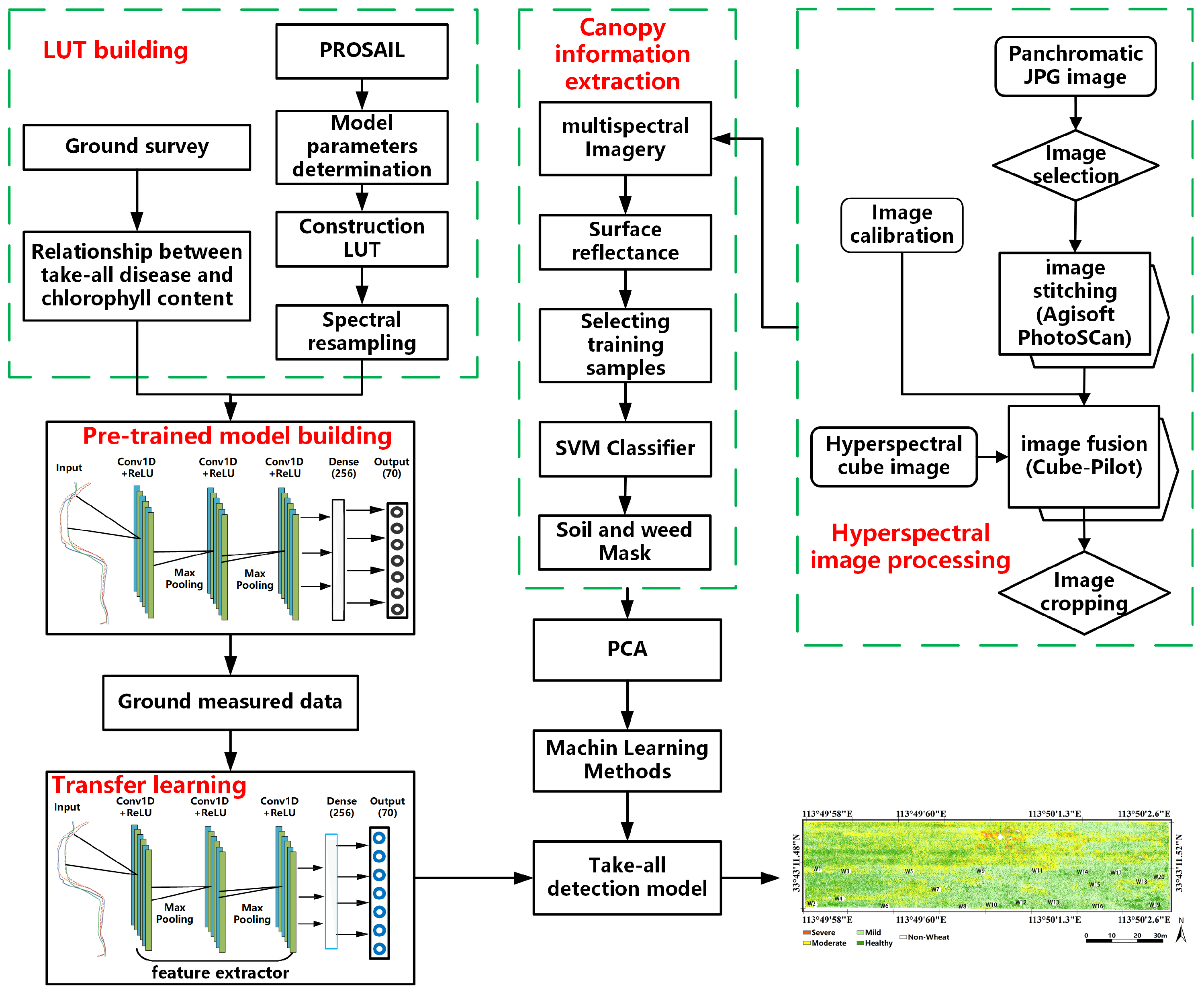
The deep learning system is a hierarchical architecture, where different layers learn different features. These layers are finally connected to a fully connected layer to obtain the final output. This hierarchical architecture allows us to use a pre-trained network with the final layer removed to act as a feature extractor for other tasks. In the transfer learning process [42], there is a large difference in the sample size between the two training periods, but there is a strong similarity between the data. Therefore, considering the overfitting problem, it is not a good idea to fine-tune the model. Therefore, we used a feature extraction approach for transfer learning [43]. We used the PROSAIL model simulation to obtain a large amount of training data, used the 1D-CNN network to obtain a pre-trained model, removed the last fully connected layer, and used the rest of the model as a fixed feature extractor for the new dataset. Finally, we used the ground truth data for transfer learning of the model to generate a new fully connected layer to improve the prediction accuracy of the model for real data. The algorithm flow is shown in Figure 3. We generated 47,040 sets of simulated data using the PROSAIL model and created a pre-trained model. To expand the usability of the pre-trained model, we employed transfer learning with feature extraction and applied it to 44 sets of measured data. This method enables the resulting model to be more widely applicable to different datasets and real-world scenarios.

2.5. Performance Metrics

The simulated results of canopy chlorophyll content were compared with the deep neural network estimates using the coefficient of determination ( R 2 ), and root mean square error ( R M S E ). The R M S E was calculated to quantify the error between the estimated and observed chlorophyll content results. The lower the R M S E is, the smaller the residual variance and the better the model effect. The R 2 value represents the degree of model fit and takes a value in the range of 0–1. The larger the value is, the better the model fit.
R M S E = 1 n i = 1 n ( y i ^ y i ) 2
R 2 = 1 i = 1 n ( y i ^ y ¯ ) 2 i = 1 n ( y i y ¯ ) 2
where n represents the number of samples, y i ^ is the predicted value of the i-th sample by the regression model, y i is the actual value of the i-th sample, and y ¯ is the mean value of all samples.

3. Results and Discussion

3.1. Modeling and Validation of Wheat Take-All

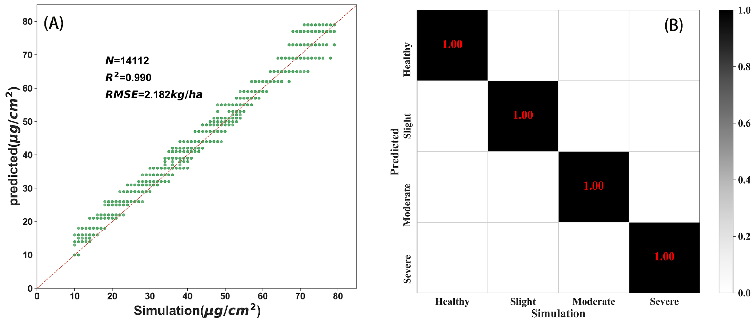
Using the simulated data from PROSAIL, the canopy reflectance curve and the take-all disease grade were used as input and output data, respectively, and the transfer learning model was trained using a ratio of 4:1 with respect to the amount of training and validation data. Figure 4 shows the validation comparison between the prediction results of the CNN model and the simulation results of the PROSAIL model. There are some differences between the prediction results of the model and the simulation results, and multiple simulation results correspond to one prediction result, but the R M S E between them is 2.631 and the R 2 is 0.732, while the probability of correctness of the classification classes for the take-all disease is 100% for both results, indicating that the classification model has high reliability.
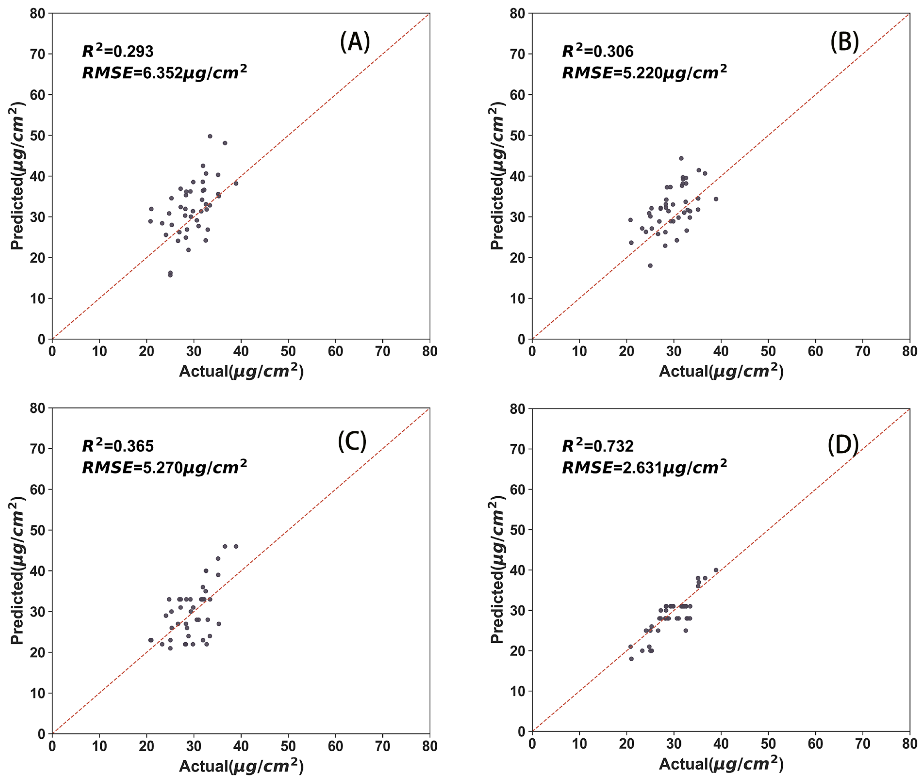
Although the model constructed using only simulated data has a certain physical basis, there may be problems in practical applications, and the hyperspectral curves acquired by the UAV may differ from the results simulated by PROSAIL. Therefore, in transfer learning, we can freeze all feature extraction layers and only adjust the weights of the fully connected layer. This method of freezing the feature extraction layer is suitable for tasks where the input data for the new task and the original task are highly similar, which allows us to fully utilize the already trained feature extraction layer on the new task, thereby speeding up the training process and improving the performance of the model. The 44 data measured on the ground were used as the new training samples to retrain the CNN model. To verify the chlorophyll inversion accuracy of the transfer learning model, the chlorophyll inversion results were compared with the ground truth data, and the results are shown in Figure 5D. There is a good linear relationship between the inverse chlorophyll content and the measured values.

3.2. Comparison of Canopy Chlorophyll Content Prediction from Different Methods

We also used some classical machine learning algorithms (partial least squares regression (PLSR), random forest [44] (RF), and support vector regression [45] (SVR)) to construct the inverse model of chlorophyll content. We chose the above methods because they are widely used and are mature regression and classification methods, which have been proven to be effective for high-dimensional and noisy data. Although LUT search is also widely used and has good interpretability, it requires a large amount of computational resources and storage space and has high requirements for preprocessing and feature extraction of input data. PLSR is a multivariate statistical data analysis method that combines the advantages of typical correlation analysis and linear regression analysis. RF is an ensemble learning method based on multiple decision trees that combines regression submodels to model a large number of interrelated input variables, and SVR is a supervised learning algorithm that finds a regression plane on which all data within the ensemble are closest to the plane. The same training is performed for the simulated data of PROSAIL, after which the trained model is validated on the ground truth data. Considering the existence of 175 bands in the hyperspectral data, we first used the principal component analysis [46,47] (PCA) method to downscale the data to 10 bands to eliminate the redundancy existing among the data bands, and the results of the three methods are shown in Figure 5, while the resultant performance metrics are presented in Table 3, where a comparison with our work is made.
The comparison of different methods showed that the accuracy of the machine learning method was significantly lower than that of the transfer learning method in chlorophyll content prediction, and the transfer learning model had the best accuracy, with R 2 and R M S E values of 0.732 and 2.631 mg/L, respectively. Although the vegetation radiative transfer model can achieve high accuracy in the inversion of canopy chlorophyll content, various factors can affect the fitting results. First, different vegetation types have different optical characteristics, so it is necessary to choose an appropriate model to improve the inversion accuracy. Secondly, it is necessary to consider and remove the influence of atmospheric and soil background to reduce interference and error. In addition, the influence of data quality also needs to be considered and processed. Finally, the selection of canopy structure and simulation parameters in the model may also affect the results. In order to improve the inversion accuracy, appropriate models and parameters should be selected according to specific conditions, and data processing and correction should be carried out to reduce errors and improve accuracy.

3.3. Spatial Distribution Results of Wheat Take-All

Based on the relationship between the chlorophyll content and take-all disease, the study area is filled with take-all disease, and the results are shown in Figure 6. It is noted that more than 60% of the image elements in the study area showed different degrees of allograft disease. By analyzing the regional inversion results, it can be seen that the disease spreads around a certain image element, which is consistent with take-all disease damage propagation.
However, potential issues exist with respect to the inversion results, which can occur due to several reasons. First, the determination of parameters is based on empirical knowledge of the model of the relationship between the chlorophyll content and wheat take-all disease. The fixed-threshold discrimination method has limitations, and errors may occur to some extent. Secondly, the hyperspectral sensor has a low signal-to-noise ratio, and changes in external conditions can easily affect the consistency of the quality of the acquired images, leading to deviation in the spectral data of the canopy from the real situation. Calibration errors of the sensor can also yield effects similar to those of random noise. External conditions, such as moisture or heavy metal stress, can cause a decrease in the chlorophyll content of the winter wheat canopy. For disease monitoring, using images from a single period for inversion has certain limitations and it is difficult to exclude the influence of some non-disease factors [48]. In the process of constructing simulated data, most parameters in the PROSAIL model use empirical values, which do not correspond to the actual situation and may cause errors when performing canopy chlorophyll inversion.
To address these issues, subsequent studies will optimize the parameters for constructing simulation data further to improve inversion accuracy. Additionally, multiple images will be used for comparisons with different periods to avoid uncertainties caused by data from a single period and to improve monitoring accuracy. In addition, both LAI and canopy chlorophyll content will be used to determine the level of wheat take-all disease, in order to avoid misjudgment caused by a fixed chlorophyll content threshold.

4. Conclusions

Considering the characteristics of hyperspectral sensor mapping, the PROSAIL model was used to construct the simulated data of winter wheat canopy chlorophyll content, and based on the relationship between the canopy chlorophyll content and take-all disease levels, the classification model between the canopy reflectance curve and take-all was obtained using a transfer learning method.
(1) The canopy chlorophyll content of wheat decreases after being infected with take-all disease, and the relationship between the canopy chlorophyll content and take-all disease levels is established based on their relationship. The classification model between the canopy reflectance curve and take-all disease is constructed using a CNN model, which can be used for remote sensing monitoring of take-all disease at a regional scale with high accuracy.
(2) The deep neural network requires a large amount of data support, and the training data are simulated data generated using the PROSAIL model. The pre-training model is generated using these data with clear physical meaning, and then the model is adjusted based on the ground measurement data using the transfer learning method of feature extraction to improve the robustness and generalization ability of the model.
For the method used in this paper, it is feasible to construct a model for monitoring take-all disease of winter wheat based on transfer learning of the canopy chlorophyll content, which has high prediction accuracy and can provide a new method for nondestructive and rapid monitoring of total erosion of wheat.

Author Contributions

Conceptualization, J.W. and H.Q.; methodology, J.W.; formal analysis, L.S.; data curation, H.Q.; writing—original draft preparation, J.W.; writing—review and editing, H.Q., L.S., Y.F., H.S. and Y.L. All authors have read and agreed to the published version of the manuscript.

Funding

This research was funded by the National Natural Science Foundation of China (NO. 42101362, 31501225); the Natural Science Foundation of Henan Province of China (NO. 222300420463); the Joint Fund of Science and Technology Research Development Program (Application Research) of Henan Province, China (222103810024).

Institutional Review Board Statement

Not applicable.

Data Availability Statement

Not applicable.

Conflicts of Interest

The authors declare no conflict of interest.

References

  1. James Cook, R. Take-all of wheat. Physiol. Mol. Plant Pathol. 2003, 62, 73–86. [Google Scholar] [CrossRef]
  2. Kwak Youn-Sig, W.D.M. Take-all of Wheat and Natural Disease Suppression: A Review. Plant Pathol. J. 2013, 29, 125–135. [Google Scholar] [CrossRef]
  3. Yuan, L.; Huang, Y.; Loraamm, R.W.; Nie, C.; Wang, J.; Zhang, J. Spectral analysis of winter wheat leaves for detection and differentiation of diseases and insects. Field Crop. Res. 2014, 156, 199–207. [Google Scholar] [CrossRef] [Green Version]
  4. Bhandari, M.; Ibrahim, A.M.; Xue, Q.; Jung, J.; Chang, A.; Rudd, J.C.; Maeda, M.; Rajan, N.; Neely, H.; Landivar, J. Assessing winter wheat foliage disease severity using aerial imagery acquired from small Unmanned Aerial Vehicle (UAV). Comput. Electron. Agric. 2020, 176, 105665. [Google Scholar] [CrossRef]
  5. Guo, A.; Huang, W.; Dong, Y.; Ye, H.; Ma, H.; Liu, B.; Wu, W.; Ren, Y.; Ruan, C.; Geng, Y. Wheat Yellow Rust Detection Using UAV-Based Hyperspectral Technology. Remote Sens. 2021, 13, 123. [Google Scholar] [CrossRef]
  6. Su, J.; Liu, C.; Coombes, M.; Hu, X.; Wang, C.; Xu, X.; Li, Q.; Guo, L.; Chen, W.H. Wheat yellow rust monitoring by learning from multispectral UAV aerial imagery. Comput. Electron. Agric. 2018, 155, 157–166. [Google Scholar] [CrossRef]
  7. Sun, Q.; Chen, L.; Xu, X.; Gu, X.; Hu, X.; Yang, F.; Pan, Y. A new comprehensive index for monitoring maize lodging severity using UAV-based multi-spectral imagery. Comput. Electron. Agric. 2022, 202, 107362. [Google Scholar] [CrossRef]
  8. Guo, W.; Zhu, Y.; Wang, H.; Zhang, J.; Dong, P.; Qiao, H. Monitoring Model of Winter Wheat Take-all Based on UAV Hyperspectral Imaging. Trans. Chin. Soc. Agric. Mach. 2019, 50, 162–169. [Google Scholar] [CrossRef]
  9. Guo, W.; Yang, Y.; Zhao, H.; Song, R.; Dong, P.; Jin, Q.; Baig, M.H.A.; Liu, Z.; Yang, Z. Winter Wheat Take-All Disease Index Estimation Model Based on Hyperspectral Data. Appl. Sci. 2021, 11, 9230. [Google Scholar] [CrossRef]
  10. Jay, S.; Maupas, F.; Bendoula, R.; Gorretta, N. Retrieving LAI, chlorophyll and nitrogen contents in sugar beet crops from multi-angular optical remote sensing: Comparison of vegetation indices and PROSAIL inversion for field phenotyping. Field Crop. Res. 2017, 210, 33–46. [Google Scholar] [CrossRef] [Green Version]
  11. Sun, J.; Wang, L.; Shi, S.; Li, Z.; Yang, J.; Gong, W.; Wang, S.; Tagesson, T. Leaf pigment retrieval using the PROSAIL model: Influence of uncertainty in prior canopy-structure information. Crop J. 2022, 10, 1251–1263. [Google Scholar] [CrossRef]
  12. Xu, L.; Shi, S.; Gong, W.; Shi, Z.; Qu, F.; Tang, X.; Chen, B.; Sun, J. Improving leaf chlorophyll content estimation through constrained PROSAIL model from airborne hyperspectral and LiDAR data. Int. J. Appl. Earth Obs. Geoinf. 2022, 115, 103128. [Google Scholar] [CrossRef]
  13. Malenovský, Z.; Homolová, L.; Zurita-Milla, R.; Lukeš, P.; Kaplan, V.; Hanuš, J.; Gastellu-Etchegorry, J.P.; Schaepman, M.E. Retrieval of spruce leaf chlorophyll content from airborne image data using continuum removal and radiative transfer. Remote Sens. Environ. 2013, 131, 85–102. [Google Scholar] [CrossRef] [Green Version]
  14. Botha, E.J.; Leblon, B.; Zebarth, B.; Watmough, J. Non-destructive estimation of potato leaf chlorophyll from canopy hyperspectral reflectance using the inverted PROSAIL model. Int. J. Appl. Earth Obs. Geoinf. 2007, 9, 360–374. [Google Scholar] [CrossRef]
  15. Sun, B.; Wang, C.; Yang, C.; Xu, B.; Zhou, G.; Li, X.; Xie, J.; Xu, S.; Liu, B.; Xie, T.; et al. Retrieval of rapeseed leaf area index using the PROSAIL model with canopy coverage derived from UAV images as a correction parameter. Int. J. Appl. Earth Obs. Geoinf. 2021, 102, 102373. [Google Scholar] [CrossRef]
  16. Qiao, L.; Tang, W.; Gao, D.; Zhao, R.; An, L.; Li, M.; Sun, H.; Song, D. UAV-based chlorophyll content estimation by evaluating vegetation index responses under different crop coverages. Comput. Electron. Agric. 2022, 196, 106775. [Google Scholar] [CrossRef]
  17. Qian, B.; Ye, H.; Huang, W.; Xie, Q.; Pan, Y.; Xing, N.; Ren, Y.; Guo, A.; Jiao, Q.; Lan, Y. A sentinel-2-based triangular vegetation index for chlorophyll content estimation. Agric. For. Meteorol. 2022, 322, 109000. [Google Scholar] [CrossRef]
  18. Atzberger, C. Object-based retrieval of biophysical canopy variables using artificial neural nets and radiative transfer models. Remote Sens. Environ. 2004, 93, 53–67. [Google Scholar] [CrossRef]
  19. Darvishzadeh, R.; Skidmore, A.; Schlerf, M.; Atzberger, C. Inversion of a radiative transfer model for estimating vegetation LAI and chlorophyll in a heterogeneous grassland. Remote Sens. Environ. 2008, 112, 2592–2604. [Google Scholar] [CrossRef]
  20. Pantazi, X.; Moshou, D.; Alexandridis, T.; Whetton, R.; Mouazen, A. Wheat yield prediction using machine learning and advanced sensing techniques. Comput. Electron. Agric. 2016, 121, 57–65. [Google Scholar] [CrossRef]
  21. Jeong, S.; Ko, J.; Yeom, J.M. Predicting rice yield at pixel scale through synthetic use of crop and deep learning models with satellite data in South and North Korea. Sci. Total Environ. 2022, 802, 149726. [Google Scholar] [CrossRef] [PubMed]
  22. Koirala, A.; Walsh, K.B.; Wang, Z.; McCarthy, C. Deep learning—Method overview and review of use for fruit detection and yield estimation. Comput. Electron. Agric. 2019, 162, 219–234. [Google Scholar] [CrossRef]
  23. Krizhevsky, A.; Sutskever, I.; Hinton, G.E. ImageNet Classification with Deep Convolutional Neural Networks. Commun. ACM 2017, 60, 84–90. [Google Scholar] [CrossRef] [Green Version]
  24. Schmidhuber, J. Deep learning in neural networks: An overview. Neural Netw. 2015, 61, 85–117. [Google Scholar] [CrossRef] [Green Version]
  25. LeCun, Y.; Bengio, Y.; Hinton, G. Deep learning. Nature 2015, 521, 436–444. [Google Scholar] [CrossRef] [PubMed]
  26. Fischer, T.; Krauss, C. Deep learning with long short-term memory networks for financial market predictions. Eur. J. Oper. Res. 2018, 270, 654–669. [Google Scholar] [CrossRef] [Green Version]
  27. Shendryk, Y.; Rist, Y.; Ticehurst, C.; Thorburn, P. Deep learning for multi-modal classification of cloud, shadow and land cover scenes in PlanetScope and Sentinel-2 imagery. ISPRS J. Photogramm. Remote Sens. 2019, 157, 124–136. [Google Scholar] [CrossRef]
  28. Ji, S.; Dai, P.; Lu, M.; Zhang, Y. Simultaneous Cloud Detection and Removal From Bitemporal Remote Sensing Images Using Cascade Convolutional Neural Networks. IEEE Trans. Geosci. Remote Sens. 2021, 59, 732–748. [Google Scholar] [CrossRef]
  29. Sun, L.; Yang, X.; Jia, S.; Jia, C.; Wang, Q.; Liu, X.; Wei, J.; Zhou, X. Satellite data cloud detection using deep learning supported by hyperspectral data. Int. J. Remote Sens. 2020, 41, 1349–1371. [Google Scholar] [CrossRef] [Green Version]
  30. Chen, J.; Jönsson, P.; Tamura, M.; Gu, Z.; Matsushita, B.; Eklundh, L. A simple method for reconstructing a high-quality NDVI time-series data set based on the Savitzky–Golay filter. Remote Sens. Environ. 2004, 91, 332–344. [Google Scholar] [CrossRef]
  31. Cortes, C.; Vapnik, V. Support-vector networks. Mach. Learn. 1995, 20, 273–297. [Google Scholar] [CrossRef]
  32. Jacquemoud, S.; Verhoef, W.; Baret, F.; Bacour, C.; Zarco-Tejada, P.J.; Asner, G.P.; François, C.; Ustin, S.L. PROSPECT+SAIL models: A review of use for vegetation characterization. Remote Sens. Environ. 2009, 113, S56–S66. [Google Scholar] [CrossRef]
  33. Berger, K.; Atzberger, C.; Danner, M.; D’Urso, G.; Mauser, W.; Vuolo, F.; Hank, T. Evaluation of the PROSAIL Model Capabilities for Future Hyperspectral Model Environments: A Review Study. Remote Sens. 2018, 10, 85. [Google Scholar] [CrossRef] [Green Version]
  34. Féret, J.B.; Gitelson, A.; Noble, S.; Jacquemoud, S. PROSPECT-D: Towards modeling leaf optical properties through a complete lifecycle. Remote Sens. Environ. 2017, 193, 204–215. [Google Scholar] [CrossRef] [Green Version]
  35. Féret, J.B.; Berger, K.; de Boissieu, F.; Malenovský, Z. PROSPECT-PRO for estimating content of nitrogen-containing leaf proteins and other carbon-based constituents. Remote Sens. Environ. 2021, 252, 112173. [Google Scholar] [CrossRef]
  36. Verhoef, W.; Bach, H. Coupled soil–leaf-canopy and atmosphere radiative transfer modeling to simulate hyperspectral multi-angular surface reflectance and TOA radiance data. Remote Sens. Environ. 2007, 109, 166–182. [Google Scholar] [CrossRef]
  37. Verhoef, W.; Jia, L.; Xiao, Q.; Su, Z. Unified Optical-Thermal Four-Stream Radiative Transfer Theory for Homogeneous Vegetation Canopies. IEEE Trans. Geosci. Remote Sens. 2007, 45, 1808–1822. [Google Scholar] [CrossRef]
  38. Atzberger, C.; Richter, K. Spatially constrained inversion of radiative transfer models for improved LAI mapping from future Sentinel-2 imagery. Remote Sens. Environ. 2012, 120, 208–218. [Google Scholar] [CrossRef]
  39. Jacquemoud, S.; Baret, F. PROSPECT: A model of leaf optical properties spectra. Remote Sens. Environ. 1990, 34, 75–91. [Google Scholar] [CrossRef]
  40. Hosgood, B.; Jacquemoud, S.; Andreoli, G.; Verdebout, J.; Pedrini, G.; Schmuck, G. Leaf Optical Properties EXperiment 93 (LOPEX93); Office for Official Publications of the European Communities, Joint Research Centre: Ispra, Italy, 1994. [Google Scholar]
  41. Wohlfahrt, G.; Bahn, M.; Tappeiner, U.; Cernusca, A. A multi-component, multi-species model of vegetation–atmosphere CO2 and energy exchange for mountain grasslands. Agric. For. Meteorol. 2001, 106, 261–287. [Google Scholar] [CrossRef]
  42. Weiss, K.R.; Khoshgoftaar, T.M.; Wang, D. A survey of transfer learning. J. Big Data 2016, 3, 9. [Google Scholar] [CrossRef] [Green Version]
  43. Bernico, M.; Li, Y.; Zhang, D. Investigation on How Data Volume Affects Transfer Learning Performances in Business Applications. arXiv 2017, arXiv:1712.04008. [Google Scholar]
  44. Breiman, L. Random Forests. Mach. Learn. 2001, 45, 5–32. [Google Scholar] [CrossRef] [Green Version]
  45. Chang, C.C.; Lin, C.J. LIBSVM: A Library for Support Vector Machines. ACM Trans. Intell. Syst. Technol. 2011, 2, 1–27. [Google Scholar] [CrossRef]
  46. Abdi, H.; Williams, L.J. Principal component analysis. WIREs Comput. Stat. 2010, 2, 433–459. [Google Scholar] [CrossRef]
  47. Xiong, Z.; Sun, D.W.; Pu, H.; Zhu, Z.; Luo, M. Combination of spectra and texture data of hyperspectral imaging for differentiating between free-range and broiler chicken meats. LWT Food Sci. Technol. 2015, 60, 649–655. [Google Scholar] [CrossRef]
  48. Berger, K.; Machwitz, M.; Kycko, M.; Kefauver, S.C.; Van Wittenberghe, S.; Gerhards, M.; Verrelst, J.; Atzberger, C.; van der Tol, C.; Damm, A.; et al. Multi-sensor spectral synergies for crop stress detection and monitoring in the optical domain: A review. Remote Sens. Environ. 2022, 280, 113198. [Google Scholar] [CrossRef]
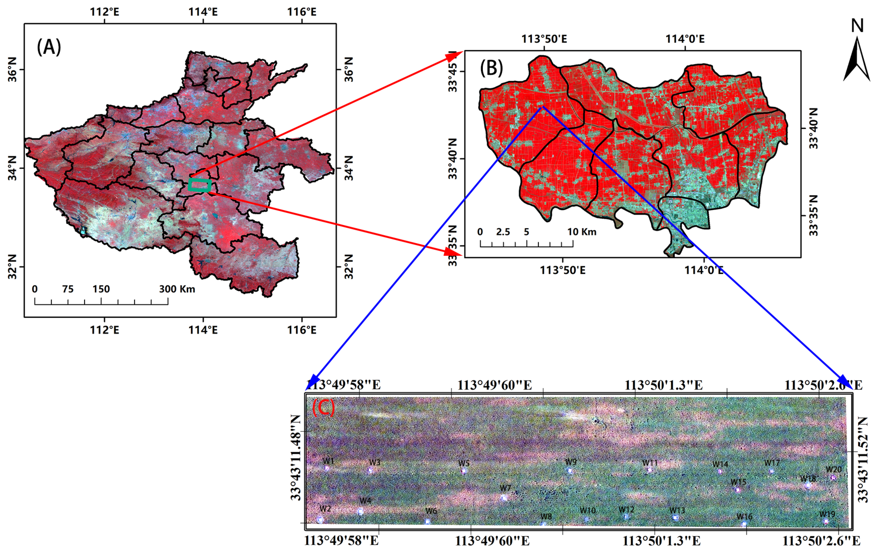
Figure 1. The geographic location of the study area. (A) False color composite map of remote sensing data in Henan Province. (B) False color composite map of remote sensing data in Luohe City. The blue box on the left is the location of the study area. (C) Color composite map of the study area (R:30, G:20, B:10). The white boxes are the sampling areas. There were 20 areas sampled.
Remotesensing 15 01960 g001
Figure 2. Map of land classification results. (A) Study area. (B) Regional RGB (R:30, G:20, B:10) image. (C) Close-up views of the corresponding winter wheat and background soil maps.
Remotesensing 15 01960 g002
Figure 3. A workflow diagram of data processing, feature extraction, and modeling.
Remotesensing 15 01960 g003
Figure 4. CNN model training results. (A) Comparison of simulated and predicted chlorophyll content in the prediction set using the CNN model. (B) Confusion matrix diagram between the prediction results using the transfer learning model and the results using the PROSAIL model.
Remotesensing 15 01960 g004
Figure 5. Comparison of multiple machine learning methods and transfer learning methods for chlorophyll content prediction. (A) PLSR. (B) RF. (C) SVR. (D) Transfer learning model.
Remotesensing 15 01960 g005
Figure 6. Spatial distribution of the disease index of wheat take-all in the study area.
Remotesensing 15 01960 g006
Table 1. The relationship between the levels of wheat take-all disease and the content of chlorophyll.
Chlorophyll Content ( μ g/cm 2 )Class
≥36Healthy
28–35Mild
21–27Moderate
≤20Severe
Table 2. The input parameters of PROSAIL.
ParameterDescription of ParameterUnitsParameter Setting
NLeaf structure parameterN/A1.5
C a b Chlorophyll a+b concentration μ g/cm 2 10–80 (SL:1)
C a r Carotenoid concentration μ g/cm 2 6
C b r o w n Brown pigment μ g/cm 2 0.1
C w Equivalent water thicknesscm0.01
C m Dry matter contentg/cm 2 0.005
LAILeaf Area Indexm 2 /m 2 1–8 (SL:0.1)
LIDFaLeaf angle distributionN/A−0.35
LIDFbLeaf angle distributionN/A−0.15
PsoilDry/Wet soil factorN/A0.5
hspotHotspot parameterN/A0.01
θ s Solar zenith angledeg25
θ v Observer zenith angledeg0
ψ Relative azimuth angledeg90
Table 3. R 2 and RMSE of the prediction in the simulation data.
PLSRRFSVROur Model
R 2 0.2930.3060.3650.732
RMSE6.3525.225.272.631
Disclaimer/Publisher’s Note: The statements, opinions and data contained in all publications are solely those of the individual author(s) and contributor(s) and not of MDPI and/or the editor(s). MDPI and/or the editor(s) disclaim responsibility for any injury to people or property resulting from any ideas, methods, instructions or products referred to in the content.