Technical Note

Effects of Atmospheric Correction on Remote Sensing Statistical Inference in an Aquatic Environment

1
Donghai Laboratory, Zhoushan 316021, China
2
Department of Marine Informatics, Ocean College, Zhejiang University, Zhoushan 316021, China
*
Author to whom correspondence should be addressed.
Remote Sens. 2023, 15(7), 1907; https://doi.org/10.3390/rs15071907
Submission received: 10 February 2023 / Revised: 30 March 2023 / Accepted: 30 March 2023 / Published: 2 April 2023

Abstract

:
Atmospheric correction (AC) plays a critical role in the preprocessing of remote sensing images. Although AC is necessary for applications based on remote sensing inversion, it is not always required for those based on remote sensing classification. Recently, remote sensing statistical inference has been proposed for evaluating water quality. However, input data for these models have always been remote sensing reflectance (Rrs), which requires AC. This raises the question of whether AC is necessary for remote sensing statistical inference. We conducted a theoretical analysis and image validations by testing 24 water bodies observed by Landsat-8 and compared their spectral probability distributions (SPDs) calculated from Rrs before and after AC (using the ACOLITE model). Additionally, we tested and found that, if we use remote sensing inference as a tool to quantitatively infer statistical parameters of a specific waterbody, it is better to perform atmospheric correction. However, if the quantitative inference is applied to a large number of water bodies and high inference accuracy is not required, atmospheric correction may not be necessary, and a quick calculation based on the strong correlations between Rrs at the surface and sensor-observed reflectance can be used as a substitute.

1. Introduction

Recently, a new remote sensing analytical method called remote sensing statistical inference, also known as ‘remote sensing inference’ or simply ‘inference’, has been proposed for remote sensing in aquatic environments [1,2]. Remote sensing inference utilizes statistical information (e.g., mean, min, max, and statistical distributions) of the image-observed optical properties (e.g., remote sensing reflectance or water-leaving radiance) of ground objects (e.g., lakes) to infer statistical information (e.g., mean, min, max, and statistical distributions) of non-optical properties (e.g., lake depth, temperature, and turbidity) of these objects. The theoretical foundations of remote sensing inference are statistical optics and radiative transfer [3,4]. Compared with the other two well-known remote sensing analytical methods, classification and inversion, it can serve as either a qualitative analysis of remote sensing classification or a quantitative analysis of remote sensing inversion. The advantage of remote sensing inference is that it not only provides a new perspective for classifying objects in images but also performs more rapidly and accurately than remote sensing inversion in evaluating the statistical features of ground objects. Remote sensing inference has been preliminarily applied in water type classification and inferring the statistical features of yellow substances in lakes [1,5].
The key information used in remote sensing inference is the statistical features of spectra in images. These statistical features include common parameters such as mean, median, standard deviation (std), minimum (min), and maximum (max), or their statistical distributions within region of interest (ROI) pixels, known as the spectral probability distribution (SPD) of an ROI object. In statistics, the SPD is equivalent to the probability distribution function and, in remote sensing, SPDs are often present as histograms of optical or spectral variables (e.g., reflectance and radiance) derived from ROI pixels. SPDs are primarily used for the classification or qualitative analysis of ground objects in remote sensing inference. In traditional remote sensing classification, the spectral curve extracted from a pixel is used to classify partial objects represented by the pixel into a specific type, while in remote sensing inference, the SPD curve of a large number of pixels of an object is used to classify the entire object to a specific type. For instance, in remote sensing in an aquatic environment, we typically classify the water in a lake pixel into turbid or clear, which means the lake could be entirely turbid or clear, or some parts of it are turbid and some are clear. However, in remote sensing inference, we use SPDs of a lake to classify it quickly as turbid or clear. We treat the lake as a whole waterbody rather than a collection of water pixels, similar to how we sometimes treat a person as a complete body instead of a collection of cells. Recent studies suggest that the skewness of the SPD is associated with the watershed status and inference models have been developed and compared to evaluate CDOM in Qiandao Lake [5].
It is known that ground spectral information derived from satellite images is distorted by the atmosphere; hence, atmospheric corrections (AC) are sometimes necessary to reduce interference [6,7,8]. Previous studies have shown that AC is not required for some applications involving remote sensing classification and change detection [9,10,11], while it is necessary for most applications involving remote sensing inversion [12,13,14,15]. In previous studies of remote sensing inference, spectral information such as SPDs was derived from atmospherically corrected water-leaving signals, such as remote sensing reflectance (Rrs), which is widely used in water color remote sensing. Because SPDs used in remote sensing inference are normalized linearly by their own scale and shift factors, it is possible that the normalized SPDs are not significantly affected by the atmosphere. However, it has not been investigated if AC is necessary for using Rrs-based normalized SPDs in remote sensing inference, as there are many other remotely sensed variables available for making SPDs, such as digital number (DN) and radiance at the top of the atmosphere (TOA), which can be obtained without AC. Retrieving Rrs from satellite images is a complicated process involving not only AC but also removing the reflective effect of the water surface. If the SPD of Rrs is the same as the SPD of DN, meaning AC is not necessary, then a lot of work can be saved in remote sensing inference applications.
The objective of this study is to conduct theoretical and image analyses to explore the effects of atmospheric correction on remote sensing statistical inference. First, we will use theoretical analysis to show that normalized SPDs should remain invariant during radiative transfer between the atmosphere and the Earth’s surface. Next, we will use image analysis to verify the accuracy of the theoretical analysis.

2. Theoretical Analysis

To compare different SPDs of various water bodies in nature, it is common practice to normalize them into the same range, because, in remote sensing inference, we focus mainly on the key statistical characteristics of SPD rather than their magnitudes. This is similar to topology, where the shape of an object is sometimes the only concern, regardless of how it is scaled or shifted. If the SPDs of two lakes are both normal distributions, but with different means and standard deviations, then the two SPDs are the same in form because one normal distribution can be scaled and shifted to the other normal distribution. In remote sensing statistical inference, max-min normalization (linear normalization) is used to scale and shift Rrs of different waters into the same range 0–1 [1,16], using the following equation:
R r s _ n o r m = R r s min ( R r s ) max ( R r s ) min ( R r s )
where Rrs_norm is the linearly normalized Rrs and max(Rrs) and min(Rrs) are the maximum and minimum Rrs, respectively, of all ROI pixels. Using Equation (1), the maximum and minimum Rrs are normalized to 1 and 0, respectively, and the other Rrs are normalized to values between 0 and 1.
The relationship between the observed radiance LTOA or reflectance RTOA and the DN measured by the satellite (e.g., Landsat-8) is given by
L T O A = g a i n × D N + o f f s e t .
where the gain and offset are sensor-specific parameters. The RTOA can be calculated using the same Equation (2) but with different gain and offset.
The LTOA can be further decomposed into three components, such that
L T O A = L p a t h + L r e f l e c t e d + L a d j a c e n c y
where Lpath is the atmospheric path radiance, Lreflected is the radiance reflected by the ground surface, and Ladjacency is the radiance reflected by the adjacent pixels. If we assume (A1) that the signals from adjacent pixels are quite small and can be ignored, and (A2) that the atmosphere is horizontally homogenous within the water of interest (WOI), which typically covers tens or hundreds of km2, then Equation (3) becomes
L T O A = L p a t h + R s u r f E d T π ( 1 R s u r f S )
where Rsurf is the surface reflectance, Ed is the total downwelling irradiance, T is the total transmittance from the surface to the sensor, and S is the spherical albedo of the atmosphere [17]. By estimating the parameters Lpath, Ed, T, and S, atmospheric corrections can predict Rsurf based on the sensor-observed LTOA. If we further assume (A3) that Rsurf × S is much smaller than 1, then Equation (4) becomes
L T O A = L p a t h + R s u r f E g T π
This equation is then converted into
R s u r f = π E d T L T O A π L p a t h E d T
In addition, water’s Rsurf is contributed by the signals reflected only from the water surface and the signals leaving the water, which are reflected by in-water components as well as by the water itself, so, to obtain Rrs, the water-surface signals must be removed using the equation
R r s = 1 π R s u r f L s u r f E d
where Lsurf is the radiance reflected by the water surface [18].
Because RTOA and Rrs are in different units, to compare them, we use the variable Rrs_TOA, defined by
R r s _ T O A = 1 π R T O A
where Rrs and Rrs_TOA are both in the unit sr−1.
Equations (2), (6) and (7) demonstrate that there are always linear transforms along the variables DN to LTOA/RTOA, Rsurf, and Rrs. Therefore, the results of their linear normalization should be invariant, as the scale and shift factors in Equations (2), (6) and (7) will be canceled out when using the normalization Equation (1).
We have theoretically proven that SPDs of linearly normalized Rrs should be approximately equal to those of the linearly normalized DN. However, this approximation depends on the above three key assumptions, (A1), (A2), and (A3), which transform Equation (3) into Equation (6). If these three assumptions—namely, (A1) the effects of adjacent pixels can be ignored, (A2) the atmosphere is horizontally homogenous, and (A3) Rsurf × S is much smaller than 1—are not true, then the SPDs of Rrs_norm may deviate significantly from the SPDs of the linearly normalized LTOA to some extent. Therefore, in the following section, we compare the SPDs of normalized Rrs and Rrs_TOA retrieved from real images to determine whether the above assumptions hold true and whether any differences can be ignored.

3. Image Data Analysis

3.1. Data and Method

Landsat-8 Level-1 images were used in this study and Rrs and RTOA in the five visible and near-infrared bands of Landsat-8, i.e., B1 (443 nm), B2 (483 nm), B3 (555 nm), B4 (665 nm), and B5 (865 nm), were obtained from 24 images (the years of their observation range from 2013 to 2019, and the months range from January to November). These images cover 24 water bodies around the world, including lakes, bays, lagoons, and estuaries (Figure 1). Note that water bodies studied by remote sensing inference should be closed and connected, so they are labelled as closed-connected water bodies [1]. While most of the lakes are closed-connected, bays, lagoons, and estuaries with narrow channels to the open sea can also be considered as approximately closed-connected.
Rrs were obtained using the ACOLITE atmospheric correction processor, which is designed for use in coastal and inland water applications. ACOLITE employs the ‘dark spectrum fitting’ approach, which automatically selects the most relevant spectral band and aerosol model [19,20,21,22]. ACOLITE supports Landsat-8. It can mask all non-water pixels in an image and calculate Rrs of all water pixels. Note that many of the known AC methods (such as iCOR, FLAASH, and 6S) were not compared in this study as they are not specifically developed for water applications and their results are only slightly different.
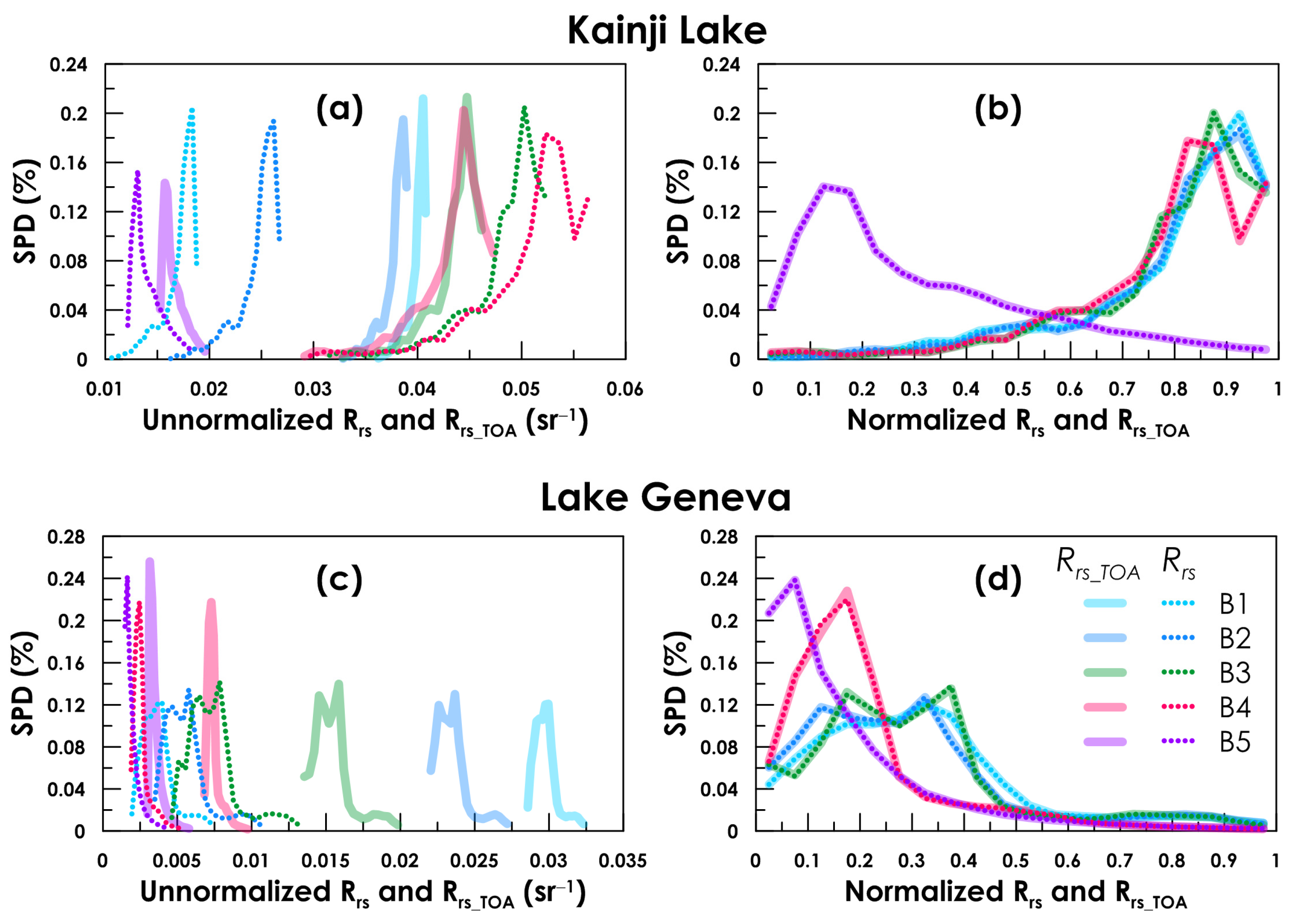
After applying the ACOLITE correction, we selected the WOI pixels in the resulting image and calculated their Rrs_norm and thus the SPD. The maximum 2% and minimum 2% Rrs within the WOI pixels were excluded from the SPD calculations, and the remaining 96% were used to construct the SPD’s histograms with bin number = 20 [1]; see SPD examples in Figure 2. As the number of WOI pixels in each water body varied, we calculated the pixel probability (the percentage of WOI pixels in each bin) rather than the raw pixel count.
The RTOA was calculated directly from the Landsat-8 DN using Equation (2), and the gains and offsets were retrieved from the image metadata files (_MTL.txt). To calculate the SPDs of RTOA, we used the exact same WOI pixels that were used to calculate the SPDs of Rrs. RTOA were also linearly normalized using the same method in Equation (1), and then SPDs of Rrs_TOA = 1 π RTOA were also calculated accordingly.
The difference between normalized Rrs and Rrs_TOA was expressed as MAPE (mean absolute percentage error) using the following formula:
M A P E = 100 % n i = 1 n | S P D ( R r s _ T O A , i ) S P D ( R r s , i ) | S P D ( R r s , i )
where SPD(Rrs, i) and SPD(Rrs_TOA, i) are the spectral probabilities (percentage counts) of Rrs and Rrs_TOA, respectively, in the i-th bin. In addition, we also calculated the RMSE (root mean squared error) and bias between the two variables to provide more information about their difference.

3.2. Results and Discussion

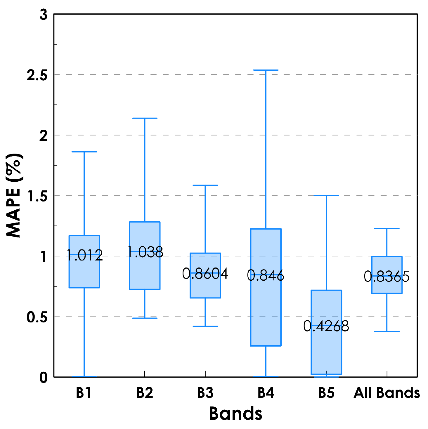
The results show that, for all 24 water bodies in the study, the overall average MAPE between the SPDs of the normalized Rrs and Rrs_TOA at five Landsat-8 bands is only 0.84% (Figure 3). This error is quite small, indicating that the SPDs of Rrs and Rrs_TOA are almost the same. Their differences in RMSE and bias were also quite small (overall average RMSE = 0.0012% and bias = 0.000059%). From the two examples in Figure 2b,d, the five respective SPD curves of Rrs and Rrs_TOA in Kainji Lake and Lake Geneva both matched perfectly well. Good agreement also occurred in the other 22 water bodies, proving the correctness of the above theoretical analysis in Section 2. The three assumptions, (A1), (A2), and (A3), are typically true, i.e., the effects of the adjacent radiance, atmospheric horizontal inhomogeneity, and multiple reflections can be ignored. When using SPDs of Rrs_norm for water quality or classification analysis, we can directly use the SPDs of linearly normalized Rrs_TOA or even DN, and it is not necessary to make atmospheric corrections to first calculate Rrs.
The highest MAPE of 1.82% was observed in a closed-connect bay in the Falkland Islands, South America; the lowest of 0.29% was observed in Lake McKerrow in New Zealand; and the median MAPE of the 24 water bodies was only 0.82%. The MAPEs at blue bands B1 and B2 were both around 1.02% and greater than the MAPEs at the green and red bands B3 and B4, which were both around 0.85%. It makes sense that the MAPE at the near-infrared band B5 is the smallest (0.43%), because the strong absorption effect of pure water at near-infrared wavelengths absorbs most of the downwelling irradiance and water appears dark at this band, thus the noise signals due to adjacent pixels and atmospheric multiple reflections would be less at B5 than at the other bands.
If we sometimes need to extract the quantitative statistical information (e.g., mean, min, and max) from the SPDs to infer the quantitative statistical information (mean, min, and max) of the water quality, do we need to make atmospheric corrections? To answer this question, we compared the unnormalized Rrs and Rrs_TOA. The results—see examples in Figure 2a,c—show that the shapes of the corresponding curves are similar but fall in different ranges (in unit sr−1) because of the effects of atmospheric path radiance. It seems that, if we stretch/squeeze and shift the SPDs of Rrs_TOA, then we get the SPDs of Rrs, which why their normalized SPDs match well; see Figure 2b,d. As the unnormalized SPDs of Rrs and Rrs_TOA were of different magnitudes, the quantitative statistical information derived from their SPDs will also be different. For example, in Lake Geneva and for band B3 (555 nm), the mean Rrs is 0.0075 sr−1, while the mean Rrs_TOA is 0.0487 sr−1 and, obviously, if we use mean Rrs_TOA to replace mean Rrs in inference models, it will bring large errors. Therefore, in order to quantitatively calculate some statistical parameters, such as the mean and median of Rrs, we need to make atmospheric corrections to remove the noise signals caused by atmospheric path radiance. It is the same as in remote sensing inversion, that is, atmospheric correction is necessary to apply inversion models to images.
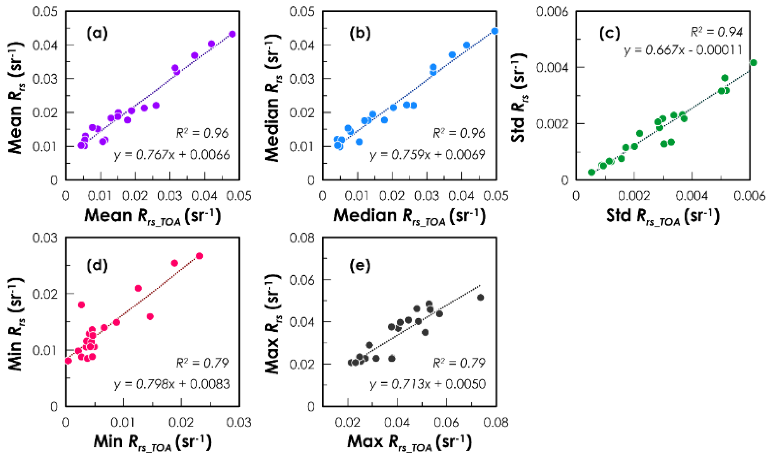
Although AC is necessary for quantitative applications of remote sensing inference, it is still a complicated task. In this study, we provide a simple method to quickly calculate the main statistical parameters (mean, median, std, min, and max) of Rrs from the same parameters of Rrs_TOA. We found that there were good correlations between the corresponding parameters of the two variables in the 24 water bodies in the study; see the results in Table 1. The overall correlation coefficient (r) of all bands and parameters is r = 0.92. For bands B3, B4, and B5, the correlations (r = 0.94, 0.95, and 0.96, respectively) were even better than the correlations for bands B1 (r = 0.86) and B2 (r = 0.89). Among the five statistical parameters, the mean, median, and std show better correlations (r = 0.95, 0.95, and 0.97, respectively) than the other two parameters, min (r = 0.87) and max (r = 0.87). These good correlations imply that we can calculate the statistical parameters of Rrs directly from the corresponding parameters of Rrs_TOA, without using the atmospheric correction to know Rrs at each pixel. We have performed the linear regressions between the respective parameters of Rrs and Rrs_TOA, so their relationships are easily expressed and the statistical parameters of Rrs can be quickly calculated using equations such as those shown in Figure 4. We suggest that, when using remote sensing inference to quantitatively study a large number of water bodies or images, we can use the above quick calculations, but when focusing on only one specific water body, atmospheric correction is needed to obtain Rrs and thus calculate its more accurate statistical parameters. Note that the empirical relationships shown in Figure 4 were only obtained from the 24 water bodies in the study, so in future work, we suggest further checking whether they apply to more water bodies or whether they need to be modified.

4. Conclusions

According to the results of using the ACOLITE model and the 24 water bodies observed from Landsat-8 images, the difference between the SPDs of normalized Rrs and Rrs_TOA is less than 1%, which means that, in remote sensing inference, if we only use linearly normalized SPDs to qualitatively classify and analyze the water types or qualities, it is not necessary to make atmospheric corrections, and SPDs can be calculated directly from the DN values. If we use statistical parameters, such as the mean, median, std, min, max, or statistical distributions of surface spectra, to quantitatively infer statistical parameters of non-optical properties of a particular water body, it is better to make atmospheric corrections. However, if the quantitative inference has been applied to a large number of water bodies for comparative analysis and inference accuracy is not a strict requirement, then atmospheric correction is sometimes not necessary. Instead, we can use the simple correlations between the corresponding statistical parameters of Rrs and Rrs_TOA to approximate the statistical parameters of Rrs—this would be much simpler and faster than using atmospheric correction.

Author Contributions

All by W.Z., except data curation by W.X. All authors have read and agreed to the published version of the manuscript.

Funding

This research was funded by the Science Foundation of Donghai Laboratory, grant number DH-2022KF01009, and the National Natural Science Foundation of China, grant number 41971373.

Data Availability Statement

Not applicable.

Conflicts of Interest

The authors declare no conflict of interest.

References

  1. Zhu, W.; Zhang, Z.; Yang, Z.; Pang, S.; Chen, J.; Cheng, Q. Spectral Probability Distribution of Closed Connected Water and Remote Sensing Statistical Inference for Yellow Substance. Photogramm. Eng. Remote Sens. 2021, 87, 807–819. [Google Scholar] [CrossRef]
  2. Zhu, W. Remote sensing statistical inference: Basic theory and forward simulation of water–air statistical radiative transfer. Earth Sci. Inform. 2021, 14, 2145–2159. [Google Scholar] [CrossRef]
  3. Goodman, J.W. Statistical Optics, 2nd ed.; John Wiley & Sons Press: Hoboken, NJ, USA, 2015. [Google Scholar]
  4. Kandidov, V. Monte Carlo method in nonlinear statistical optics. Uspekhi Fiz. Nauk. 1996, 166, 1309–1338. [Google Scholar] [CrossRef] [Green Version]
  5. Zhu, W.; Yang, Z.; He, S.; Cheng, Q. Skewness-Based Classification and Environmental Indication of Spectral Probability Distribution of Global Closed Connected Waters. IEEE Geosci. Remote Sens. Lett. 2022, 19, 1–5. [Google Scholar] [CrossRef]
  6. Kondratyev, K.Y.; Kozoderov, V.V.; Smokty, O.I. Remote Sensing of the Earth from Space: Atmospheric Correction; Springer: Berlin/Heidelberg, Germany, 1992. [Google Scholar] [CrossRef]
  7. Chavez, P.S. Image-Based Atmospheric Corrections Revisited and Improved, Photogrammetric Engineering and Remote Sensing; Springer: Berlin/Heidelberg, Germany, 1996; Volume 62, pp. 1025–1036. [Google Scholar]
  8. Emberton, S.; Chittka, L.; Cavallaro, A.; Wang, M. Sensor Capability and Atmospheric Correction in Ocean Colour Remote Sensing. Remote Sens. 2015, 8, 1. [Google Scholar] [CrossRef] [Green Version]
  9. Song, C.H.; Woodcock, C.E.; Seto, K.C.; Lenney, M.P.; Macomber, S.A. Classification and change detection using Landsat TM data: When and how to correct atmospheric effects? Remote Sens. Environ. 2001, 75, 230–244. [Google Scholar] [CrossRef]
  10. Lin, C.; Wu, C.-C.; Tsogt, K.; Ouyang, Y.-C.; Chang, C.-I. Effects of atmospheric correction and pansharpening on LULC classification accuracy using WorldView-2 imagery. Inf. Process. Agric. 2015, 2, 25–36. [Google Scholar] [CrossRef] [Green Version]
  11. Vanonckelen, S.; Lhermitte, S.; Van Rompaey, A. The effect of atmospheric and topographic correction on pixel-based image composites: Improved forest cover detection in mountain environments. Int. J. Appl. Earth Obs. Geoinf. 2015, 35, 320–328. [Google Scholar] [CrossRef]
  12. Campbell, G.; Phinn, S.R.; Dekker, A.G.; Brando, V.E. Remote sensing of water quality in an Australian tropical freshwater impoundment using matrix inversion and MERIS images. Remote Sens. Environ. 2011, 115, 2402–2414. [Google Scholar] [CrossRef] [Green Version]
  13. McCarthy, S.C.; Gould, R.W.; Richman, J.; Kearney, C.; Lawson, A. Impact of Aerosol Model Selection on Water-Leaving Radiance Retrievals from Satellite Ocean Color Imagery. Remote Sens. 2012, 4, 3638–3665. [Google Scholar] [CrossRef] [Green Version]
  14. Liu, G.; Li, Y.M.; Lyu, H.; Wang, S.; Du, C.G.; Huang, C.C. An improved land target-based atmospheric correction method for Lake Taihu. IEEE J. Sel. Top. Appl. Earth Obs. Remote Sens. 2016, 9, 793–803. [Google Scholar] [CrossRef]
  15. Zhu, W.; Tian, Y.Q.; Yu, Q.; Becker, B.L. Using Hyperion imagery to monitor the spatial and temporal distribution of colored dissolved organic matter in estuarine and coastal regions. Remote Sens. Environ. 2013, 134, 342–354. [Google Scholar] [CrossRef]
  16. Dodge, Y. The Oxford Dictionary of Statistical Terms, 6th ed.; Oxford University Press: Oxford, UK, 2006. [Google Scholar]
  17. Liang, S.L. Quantitative Remote Sensing of Land Surfaces; John Wiley & Sons, Inc.: Hoboken, NJ, USA, 2004. [Google Scholar]
  18. Mobley, C.D. Light and Water: Radiative Transfer in Natural Water; Academic Press: San Diego, CA, USA, 1994. [Google Scholar]
  19. Vanhellemont, Q.; Ruddick, K. Atmospheric correction of metre-scale optical satellite data for inland and coastal water applications. Remote Sens. Environ. 2018, 216, 586–597. [Google Scholar] [CrossRef]
  20. Vanhellemont, Q. Adaptation of the dark spectrum fitting atmospheric correction for aquatic applications of the Landsat and Sentinel-2 archives. Remote Sens. Environ. 2019, 225, 175–192. [Google Scholar] [CrossRef]
  21. Vanhellemont, Q. Sensitivity analysis of the dark spectrum fitting atmospheric correction for metre- and decametre-scale satellite imagery using autonomous hyperspectral radiometry. Opt. Express 2020, 28, 29948–29965. [Google Scholar] [CrossRef] [PubMed]
  22. Vanhellemont, Q.; Ruddick, K. Turbid wakes associated with offshore wind turbines observed with Landsat 8. Remote Sens. Environ. 2014, 145, 105–115. [Google Scholar] [CrossRef] [Green Version]
Figure 1. Map of the water bodies in the study.
Remotesensing 15 01907 g001
Figure 2. Normalized and unnormalized Rrs and Rrs_TOA of Lake Geneva and Kainji Lake: (a,c) unnormalized Rrs and Rrs_TOA and (b,d) normalized Rrs and Rrs_TOA.
Remotesensing 15 01907 g002
Figure 3. Errors (MAPEs) between linearly normalized Rrs and Rrs_TOA for the 24 water bodies in five Landsat-8 bands.
Remotesensing 15 01907 g003
Figure 4. Relationships between the statistical parameters ((a) mean, (b) median, (c) std, (d) min, and (e) max) of unnormalized Rrs and Rrs_TOA for the 24 water bodies at the B3 band (555 nm) of Landsat-8.
Remotesensing 15 01907 g004
Table 1. Correlation coefficients between the statistical parameters of unnormalized Rrs and Rrs_TOA for the 24 water bodies at five Landsat-8 bands and the averages for all five bands and five parameters. The p-values of their correlations, with the orders of 10−12 to 10−14, are much smaller than 0.05.
Stat. Para.B1B2B3B4B5Average
Mean0.880.930.980.980.970.95
Median0.880.930.980.990.970.95
Std0.950.950.970.980.980.97
Min0.750.790.890.890.980.87
Max0.810.850.890.920.890.87
Average0.860.890.940.950.960.92
Disclaimer/Publisher’s Note: The statements, opinions and data contained in all publications are solely those of the individual author(s) and contributor(s) and not of MDPI and/or the editor(s). MDPI and/or the editor(s) disclaim responsibility for any injury to people or property resulting from any ideas, methods, instructions or products referred to in the content.