Sequential Seismic Anisotropic Inversion for VTI Media with Simulated Annealing Algorithm Aided by Adaptive Setting of Optimization Parameters

Abstract

As an important geophysical data processing technique, seismic inversion estimates subsurface rock properties with seismic observations. However, anisotropic inversion, intended for a vertical transverse isotropy (VTI) media that primarily describes shale gas/oil resources, suffers from high nonlinearity. Simulated annealing is a widely used global optimization algorithm for solving nonlinear seismic inverse problems, but it involves multiple optimization parameters (e.g., initial temperature, search limit, and perturbation range). The importance of such parameters has been proven whilst the relevant analysis is limited in seismic inversion studies. This work hereby proposes a sequential anisotropic inversion method for VTI media, wherein we combine Bayesian linear and simulated annealing nonlinear inversion schemes. The simulated annealing is featured by adaptive optimization parameters aided by the linear result. Rather than the conventional method, the adaptive setting can be implemented trace by trace for complex reservoirs, which endows the method with enhanced stability and extended applicability. Synthetic tests and practical application demonstrate the validity of the method, wherein the obtained stiffness parameters facilitate the characterization of potential shale reservoirs with an improved accuracy.

1. Introduction

Prestack AVO/AVA (amplitude variation with offset/angle) seismic inversion aims to quantitatively explore the information of subsurface elastic (e.g., longitudinal and transverse wave velocities, density, anisotropy, etc.) [1,2,3,4,5,6,7,8] or petrophysical parameters (e.g., porosity, fluid saturation, mineral content, etc.) [9,10,11,12,13] and then provides a database for geofluid identification, lithology classification, and reservoir prediction [14]. By using the processed seismic gathers as input data and geological or logging data as prior constraints, it is one of the most effective techniques in seismic exploration of the oil/gas industries.

Under the assumption of an isotropic media, the traditional prestack AVO/AVA inversion achieved great successes for wide applications in sandstone hydrocarbon reservoir exploration. However, some of the highly promising unconventional resources, such as shale gas and coalbed methane, are currently considered the most important alternative resources [15]. Influenced by the oriented clay particles or horizontal laminar structures [16], most shale and coal may exhibit the vertical transverse isotropy (VTI) anisotropic characteristics [17,18], of which the seismic wavefield responses are significantly different from those of conventional sandstones [19,20]. Therefore, seismic inversions based on anisotropy theory are expected for the exploration of such unconventional reservoirs.

For the AVO/AVA modeling of VTI media, Carcione [21], Graebner [22], Schoenberg, and Protázio [23] gave the exact expressions for the corresponding reflection coefficients, which are functions of the elastic stiffness parameters. Thomsen [24] defined the three parameters, ε, δ, and γ, in order to characterize the anisotropy features of a VTI media. Then, under the assumption of weak anisotropy, Rüger [25,26] derived a simplified expression for the reflection coefficient as a function of the three Thomsen’s parameters. Due to the simple and linear forms, the Rüger approximation and its modified forms have become the widely used reflection coefficient expressions for AVO/AVA inversion of VTI media [27,28,29,30,31]. However, these approximations have lower accuracy at large incidence angles and are restricted to the assumptions of weak anisotropy and weak impedance contrasts, which limit the accuracy and applicability of the corresponding inversions [32,33]. The forward operator is a key factor of the inversion and significantly affects the result. It is therefore recommended to employ the exact formulation of the reflection coefficients to improve the accuracy of the VTI inversion. However, the solution to the inverse problem is difficult to obtain analytically, due to the high nonlinearity of the exact-equation-based forward operator. In addition, compared to the isotropic inversions (with three target parameters), the VTI inverse problem involve more unknown parameters (five or even more), leading to higher ill-posedness and thus more difficulties in practice [28,30,33]. To this end, the global optimization algorithm is an important approach for solving the prestack inversion problems.

Simulated annealing (SA), a Monte Carlo based heuristic algorithm, has the advantage of overstepping local extremes for highly nonlinear inverse problems, and is one of the most widely applied global optimization algorithms [34,35,36]. SA is proposed because of the similarity between the annealing process of solids and general optimization problems. The algorithm is featured by the probabilistic acceptance of candidate solutions according to the Metropolis criterion for achieving a global optimal solution. Rothman [37] initially introduced SA into the geophysical field to solve the residual static correction problem for seismic data processing. Since then, SA has been extended to the field of seismic inversion due to its robustness and reliability [38]. However, SA involves a variety of optimization parameters (e.g., the initial temperature, the search limit, and the perturbation range of model parameters, etc.), the settings of which have an important influence on the inversion result [39]. At present, these optimization parameters are basically set by trial and error approaches and adjusted by inversion tests with synthetic or borehole-side seismic traces, which are highly empirical and prone to an unstable result. Attempts have been made for the quantitative setting of optimization parameters. Basu and Frazer [40] suggested that a higher initial temperature and smaller damping coefficient contribute to the mature convergence of the inversion process. Aarts and Korst [41] proposed to determine the initial temperature according to the first acceptation probability. However, the reported works mainly focus on the setting of initial temperature. The relevant studies on setting optimization parameters are still limited for solving seismic inversion problems. There are fewer studies on comprehensively initializing such parameters, especially for the anisotropic inversion, which should adaptively and properly initialize multiple optimization parameters to improve the accuracy of final result.

Since the anisotropic inversion for VTI media is complicated in comparison to the conventional prestack inversions [33], it is important to reduce the artificial interferences and improve the stability and applicability of the algorithm. In this work, we presented a sequential inversion method for VTI media by combining the Bayesian linear and SA-based nonlinear inversion approaches. In particular, the optimization parameters are adaptively initialized aided by the linear inversion result for the SA algorithm. The proposed method aims to improve the simultaneous estimation of the four elastic stiffness parameters (c₃₃, c₅₅, c₁₁, and c₅₅) with enhanced stability and applicability. Although the commonly used Rüger approximation has limited accuracy at large angle ranges and strong impedance contrasts, the approximation-based linear inversion is convenient for implementing with high efficiency. Therefore, such linear results can provide a preliminary model to assist the optimization parameter estimation of the subsequent SA nonlinear inversion. For the nonlinear inversion, Graebner’s exact formulation [22] is introduced as the forward operator to improve the accuracy and applicability. The VTI inversion requires simultaneous estimations of five target parameters, which leads to an inverse problem with higher ill-posedness and more local minima. Since it is difficult to solve using the commonly used linear optimization, the SA algorithm aided by the adaptive optimization parameter setting is adopted to solve the inverse problem. The sequential inversion process includes two steps: the Rüger approximation based Bayesian linear inversion, followed by the SA nonlinear inversion based on Graebner’s exact formulation. In the first step, the preliminary estimations of the stiffness parameters can be obtained efficiently using the linear anisotropic inversion. Then, based on the preliminary result, the initial temperature and perturbation ranges can be obtained quantitatively according to the local potential energy trace by trace, and the search limit (solution space) that depends on the preliminary result can also be properly reduced, all of which is used to initialize the subsequent SA nonlinear inversion (the second step). This sequential scheme aims to improve the stability of the optimization process and the accuracy of the final result for seismic anisotropic inversion.

The paper is organized as follows. First, we present the theory of the proposed sequential anisotropic inversion method, including Graebner’s exact formulation of the reflection coefficients of the VTI media, the nonlinear inversion with the fast simulated annealing algorithm, and the adaptive optimization parameter setting aided by the linear Rüger approximation based linear inversion. Then, according to the synthetic data tests, we analyze the influences of the initial temperature, the perturbation range, and the search limit on the accuracy of inversion results. Finally, the proposed method is tested by using both synthetic data and field data applications, which demonstrate the validity of the sequential inversion scheme for anisotropic multi-parameter inversion.

2. Theory

2.1. Forward Modeling for VTI Media

Based on the convolution model, the synthetic record d can be obtained by multiplying a reflection/transmission coefficient vector ${R}\left({m},\theta \right)$ with a wavelet matrix W as follows:

$$d=G\left(m\right)+e=W\cdot R\left(m,\theta \right)+e$$

(1)

where $G\left(m\right)$ represents the forward operator and e is a vector of random noise. $R={\left[R_{PP},R_{PS},T_{PP},T_{PS}\right]}^{\mathrm{{\rm T}}}$ contains the reflection coefficients of PP ($R_{PP}$) and PS ($R_{PS}$), and the transmission coefficients of PP ($T_{PP}$) and PS ($T_{PS}$). For an interface separating two VTI media, the exact analytical expression of R is a function of the elastic parameters m (including four elasticities of c₁₁, c₁₃, c₃₃, and c₅₅, density ρ), and the incidence angle $\theta$ [22], which can be computed by

$$S\cdot R=b$$

(2)

with

$$S=\left[\begin{array}{cccc}{𝓁}_P^U& n_S^U& -{𝓁}_P^L& -n_S^L\\ n_P^U& -{𝓁}_S^U& n_P^L& -{𝓁}_S^L\\ a^U& b^U& a^L& b^L\\ d^U& e^U& -d^L& -e^L\end{array}\right]\mathrm{and}b=\left[\begin{array}{c}-{𝓁}_P^U\\ n_P^U\\ a^U\\ -d^U\end{array}\right]$$

(3)

where the superscripts U and L represent the parameters of the upper and lower layers, respectively, and the subscripts P and S denote the P- and S-wave modes, respectively. The specific expressions of the components ($a^{\ast }$, $b^{\ast }$, $d^{\ast }$, and $e^{\ast }$, with $\ast =U,L$) of Equation (3) are given in Appendix A.

2.2. Prestack Seismic Anisotropic Inversion

In the prestack seismic inversion, an objective function is set up and solved by an optimization method. However, due to the presence of noise and the nonlinearity of the forward operator, the inverse problem is ill-posed. The regularization techniques are commonly introduced to mitigate the ill condition. Based on the Bayes’ theorem [42], the objective function can be derived as follows (see Appendix B):

$$\begin{array}{ll}P\left(m|d\right)=& \frac{1}{\sqrt{2\pi \left|{\Sigma }_e\right|}}\cdot \exp \left[{\left(d-G\left(m\right)\right)}^{\mathsf{{\rm T}}}{\Sigma }_e^{-1}\left(d-G\left(m\right)\right)\right]\\ & \cdot \frac{1}{{\left(2\pi \left|{\Sigma }_m\right|\right)}^{n/2}}\cdot \exp \left[{\left(m-\overline{m}\right)}^{\mathsf{{\rm T}}}{\Sigma }_m^{-1}\left(m-\overline{m}\right)\right]\end{array}$$

(4)

where $P\left(m|d\right)$ denotes the posterior probability. The model parameter vector m includes five target parameters of the anisotropic inversion, namely the elastic stiffnesses c₁₁, c₁₃, c₃₃, and c₅₅, and the density ρ. ${\Sigma }_m$ represents the covariance matrix of the model parameters $m$, the expression of which is given in Appendix B. ${\Sigma }_e$ is the covariance matrix of the random noises. Maximizing Equation (4) leads to the estimation of unknown parameters $m$, which can be treated with minimizing the objective function of

$$J\left(m\right)={\left(d-G\left(m\right)\right)}^{\mathsf{{\rm T}}}{\Sigma }_e^{-1}\left(d-G\left(m\right)\right)+\lambda {\left(m-\overline{m}\right)}^{\mathsf{{\rm T}}}{\Sigma }_m^{-1}\left(m-\overline{m}\right)$$

(5)

where $\lambda$ is a trade-off regularization parameter, which is introduced to balance the data and the prior terms during inversion process.

2.3. Optimization Method Based on Fast Simulated Annealing

The inversion procedure is an optimization approach minimizing the objective function of Equation (5). By considering the highly nonlinear forward modeling (the relations between subsurface property parameters and survey data), the simulated annealing is a widely adopted global optimization algorithm to achieve the optimal solution for seismic inversion problems [43,44]. Compared to linear optimization, the algorithm is capable of jumping out of local minima. In this work, following the classic form of fast simulated annealing (FSA) [34,35], we derive the perturbation/update of a model parameter in the k-th iteration as

$$m_{k+1}=m_k+T_k\mathrm{sign}\left(\xi -0.5\right)\lfloor {\left(1+1/T_k\right)}^{\left|2\cdot \xi -1\right|}-1\rfloor \Delta m$$

(6)

where $m_{k+1}$ and $m_k$ are the perturbed and present model parameters, respectively. $\Delta m$ represents the perturbation range, by which the step/size of model update at each iteration is restricted. $\mathrm{sign}\left(\cdot \right)$ represents the sign function and $\xi$ is a random number between 0 and 1. $T_k$ denotes the present temperature at the k-th iteration, which starts with the pre-defined initial temperature $T_0$. The temperature gradually reduces based on the cooling schedule,

$$T_k=T_0\exp \left(-\beta k^{1/N}\right)$$

(7)

where β denotes the damping coefficient and is commonly set as a constant, N represents the dimension of model parameters (for VTI anisotropic inversion, N equals to 5). At the k-th iteration, we may accept the perturbation m_k+1 conditionally according to the acceptance probability $P_k$ as

$$P_k\left(m_k\to m_{k+1}\right)=\left\{\begin{array}{cc}1,& \Delta E<0\\ \exp \left(-{\left(\Delta E\right)}_k/T_k\right),& \Delta E>0\end{array}\right.$$

(8)

where $\Delta E$ denotes the energy difference between the objective functions with the present and perturbed model parameters at the k-th iteration. According to the defined Markov chain length, the procedure may be repeated several times until the maximum iteration number is reached.

2.4. Adaptive Optimization Parameter Setting

Although the SA algorithm has advantages for solving nonlinear inverse problems, it involves with a variety of optimization parameters, among which the search limit, perturbation range, and initial temperature directly determine the convergence of the optimization process and thereby influence the accuracy of inversion results. Therefore, we propose a sequential prestack seismic inversion based on the FSA algorithm with an adaptive optimization parameter setting, the procedure of which is described in Algorithm 1 and Figure 1. In the following, the algorithm is summarized: (1) set the initial mean and covariance matrix of the five parameters for the linear inversion according the well log data; (2) perform the linear inversion based on the Rüger approximation to generate the preliminary result (linear result); (3) set the linear result as the initial model for the subsequent FSA inversion and set up the prior term; (4) estimate the initial temperature, perturbation ranges, and search limits of FSA trace by trace with the linear inversion result; (5) obtain the final result by using the FSA nonlinear optimization approach.

2.4.1. Linear Inversion Based on the Rüger Approximation

The linear inversion by the Rüger approximation is a commonly used method to estimate the elastic parameters for VTI media, e.g., shale rocks, etc. [26,28,30]. Such a linear method has high computational efficiency; however, it obtains inverted results with limited accuracy due to the simplified forward engine with the linear optimization. Although the linear inversion results deviate from the true models to some extent, they can still provide assistances or prior information for a subsequent nonlinear inversion. Therefore, we propose to adopt the Rüger approximation based linear inversion as the first step of the sequential scheme.

In the Rüger approximation based linear inversion, the inverted parameter vector is set as $x$, including P-wave velocity v_P, S-wave velocity v_S, density ρ, and the two Thomsen’s anisotropic parameters, ε and δ. A discrete version of the reflection coefficient r is performed.

$$r=ADx$$

(9)

where the matrix $A$ is defined with the coefficients $A_{v_P}\left(\theta \right)$, $A_{v_S}\left(\theta \right)$, $A_{\rho }\left(\theta \right)$, $A_{\epsilon }\left(\theta \right)$, and $A_{\delta }\left(\theta \right)$ (see Appendix C), and $D$ is the first-order difference matrix. The corresponding synthetic record can be obtained by the convolution model as

$$d=Fx+e=WADx+e$$

(10)

where the matrix $F$ represents the forward operator, and $W$ is a wavelet matrix at a certain incidence angle. According to Buland and Omre [42], the explicit analytical solution of the inverse problem is derived based on the Bayesian framework,

$${\mathsf{\mu }}_{x|d}={\mathsf{\mu }}_x+{\left(F{\Sigma }_x\right)}^{\mathsf{{\rm T}}}{\left(F{\Sigma }_x{F}^{\mathsf{{\rm T}}}+{\Sigma }_e\right)}^{-1}\left(d-F{\mathsf{\mu }}_x\right)$$

(11)

where ${\mathsf{\mu }}_x$ and ${\Sigma }_x$ are the expectation and covariance matrices of $x$, respectively, which can be estimated with well log data, and ${\mathsf{\mu }}_{x|d}$, the posterior expectation, corresponds to the linear inversion result.

Based on the aforementioned inversion result, namely, v_P, v_S, ρ, ε, and δ, we can obtain the four stiffness parameters according to following equations [32]:

$$c_{33}=v_P^2\rho ,c_{55}=v_S^2\rho ,c_{11}=\left(2\epsilon +1\right)v_P^2\rho$$

(12)

$$c_{13}={\left[2\delta {\rho }^2{v}_P^2\left(v_P^2-v_S^2\right)+{\rho }^2{\left(v_P^2-v_S^2\right)}^2\right]}^{\frac{1}{2}}-\rho v_S^2$$

(13)

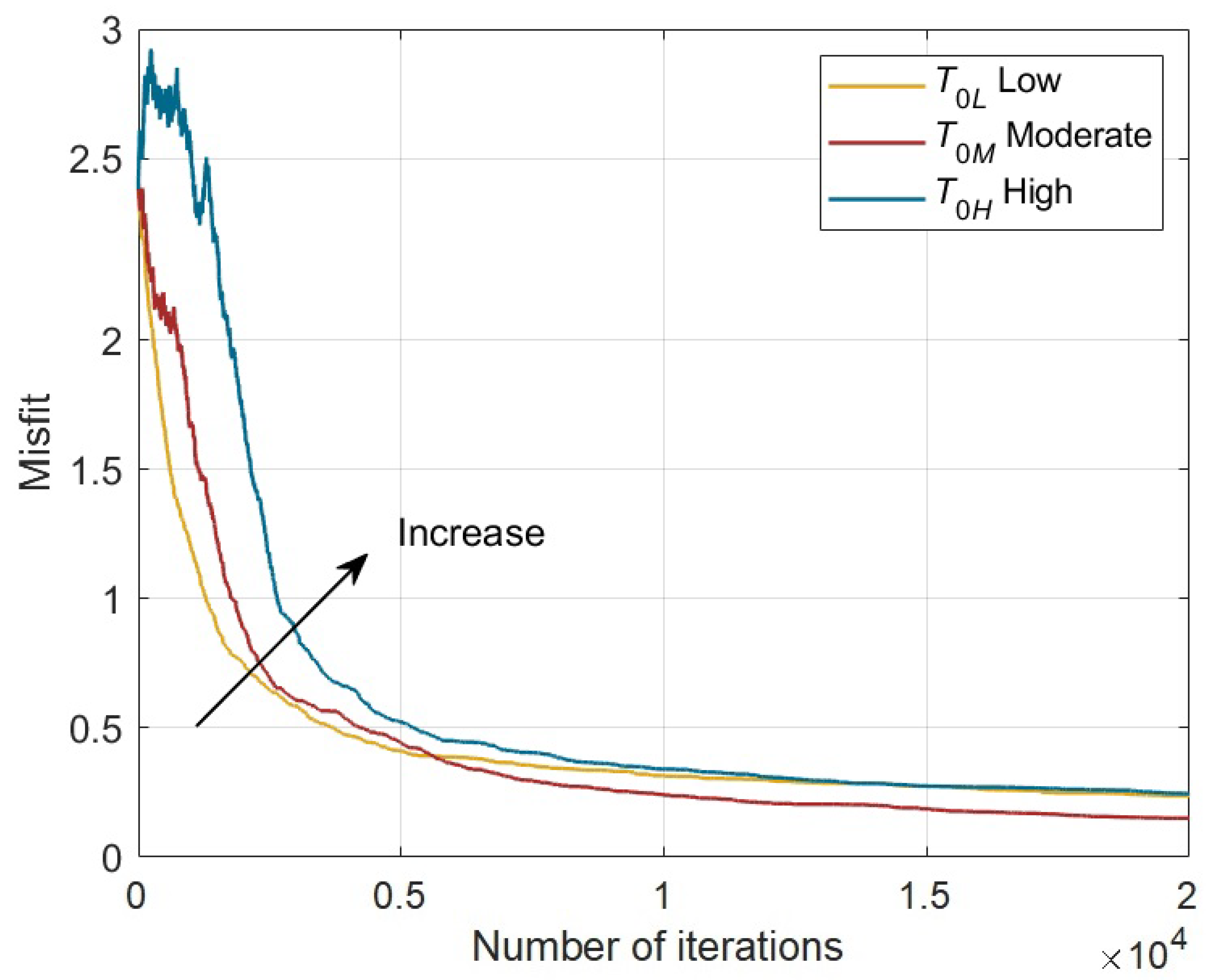
2.4.2. Initial Temperature Setting

For the traditional nonlinear inversion methods, the initial temperature is commonly set as a constant for all seismic traces, according to trial and error from models or logging data tests. Such an empirical setting may introduce errors, and it is difficult to obtain an optimal initial value for nonlinear seismic inversion. The temperature initialization therefore cannot be adaptively adjusted, which should change trace by trace with the input data condition for 2D/3D field applications. In this work, we propose to adaptively estimate the initial temperature according to the local energy variation aided by the linear inversion result, as

$$T_{0,i}=-\frac{{\displaystyle \sum _{k=1}^{N_{\mathrm{est}}}\left[J\left(m_{i,k}\right)-J\left({\left(m_L\right)}_i\right)\right]}}{N_{\mathrm{est}}\cdot \ln \left(P_{0,i}\right)}$$

(14)

where i denotes the i-th trace of model with i = 1, 2, ..., i_max, k is the k-th iteration with k = 1, 2, ..., N_est, with N_est denotes the iteration number for the estimation, which is set as 1000 in practice. The local energy is associated with the objective function value for the model parameters within a specific area (e.g., a seismic trace). The local energy variation is controlled by the temperature, which essentially determines the acceptance probability. We obtain the values of the objective function $J_{i,k}\left(m_{i,k}\right)$ and $J_i\left(m_L\right)$ by substituting the perturbed model at the i-th trace and the k-th iteration, $m_{i,k}$, and the linear result at the i-th trace, ${\left(m_L\right)}_i$, into Equation (5), respectively. $P_{0,i}$ is the initial acceptance probability, which is expected to be large (~0.95).

In practice, the perturbation of $m_{i,k}$ in the estimation cannot follow Equation (6) since the initial temperature is unknown. The perturbation is thus simplified as

$$m_{i,k+1}=m_{i,k}+\mathrm{sign}\left(\xi -0.5\right)\Delta m$$

(15)

2.4.3. Search Limit and Perturbation Range Setting

Setting the suitable search limit and perturbation range for nonlinear inversion is a key factor to accelerate the convergence and improve the result. The limits denoted by $\left[m_{\min }^{},m_{\max }^{}\right]$ are expected to be small and at the same time cover all possible solution spaces. With m_j representing the model parameter at the j-th depth point, and based on the linear result, we set the search limit as

$$m_{\min ,j}^{}=\left\{\begin{array}{ll}\left(1-2b\right)m_{L,j},& \left(m_{R,j}-m_{L,j}\right)<b{m}_{L,j}\\ \left(1-2b\right)m_{R,j}-2b\left(m_{R,j}-m_{L,j}\right),& \left(m_{R,j}-m_{L,j}\right)\ge b{m}_{L,j}\end{array}\right.$$

(16)

$$m_{\max ,j}^{}=\left\{\begin{array}{ll}\left(1+2b\right)m_{L,j},& \left(m_{R,j}-m_{L,j}\right)<b{m}_{L,j}\\ \left(1+2b\right)m_{R,j}+2b\left(m_{R,j}-m_{L,j}\right),& \left(m_{R,j}-m_{L,j}\right)\ge b{m}_{L,j}\end{array}\right.$$

(17)

where $m_{L,j}$ is the inversion result of the linear optimization, and $m_{R,j}$ denotes a true value at the same depth point extracted from reference well data. A scale coefficient b is set to vary with the relative variation of the inverted parameter. The size of search limit depends on the accuracy of the linear result, $m_{L,j}$. When the linear result is less different from the reference true value, a smaller window can be obtained according to Equations (16) and (17), while a wider search window can be obtained when the result contains many anomalies.

The perturbation range $\Delta m$ is important for updating model parameters in Equation (6). An overlarge range may cause an unstable inversion process, whilst a small range may cause the model parameter unable to reach the global optimal solution. We set the perturbation range according to the linear result, and the range is the mean of maximum and minimum values of the result at each trace,

$$\Delta m_j=\frac{1}{2}\left[\max \left(m_{L,j}\right)-\min \left(m_{L,j}\right)\right]$$

(18)

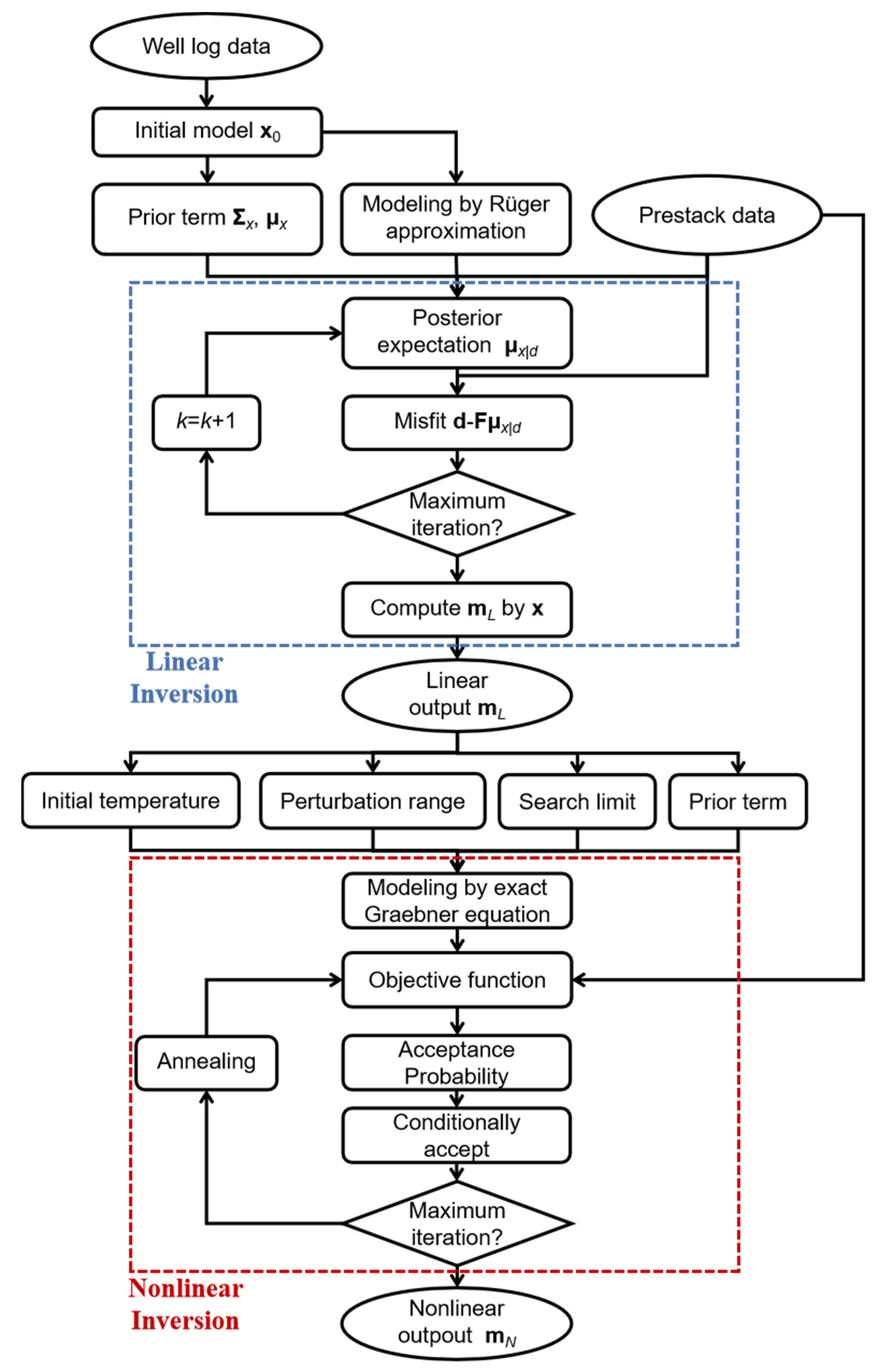
Algorithm 1 The Proposed Sequential Prestack Anisotropic Inversion Method

1. Input: the observed prestack seismic data d, and the logging data

2. Initialization for linear inversion:

2-1. Initialize the model vector for the linear inversion, and we obtain x0 = [vP0, vS0, ρ0, ε0, δ0]

2-2. Initialize the initial statistical relations among the five parameters from x0, and we obtain Σx0 and μx0 of Equation (11)

3. Stage 1 linear inversion

Adopt Equation (11) and start the loop: k = 1, 2, 3, ... do

3-1. Compute the synthetic data based on the initial model by using the Rüger approximation of Appendix C and the forward operator matrix F according to Equation (10)

3-2. Calculate the posterior expectation μx|d according to Equation (11)

3-3. Compute the misfit d-μd. Output the inversion result x = μx|d if the maximum iteration is reached, or x0 = μx|d, and repeat steps 2–3

3-4. Compute the model vector mL = [c33L,c55L,c11L,c13L,ρL] according to Equation (12) based on x

4. Preliminary output: the result mL of the first step

5. Initialization for nonlinear inversion:

5-1. Set m0 = mL as the initial model of the nonlinear inversion

5-2. Initialize the statistical relations among the five target parameters from m0, and we obtain Cm0 and $\overline{\mathbf{m}}$ of Equation (5)

5-3. Generate the initial temperature according to Equation (13) based on m0

5-4. Generate the search limit and perturbation range according to Equations (16) and (17) based on m0

6. Stage 2 nonlinear inversion:

Adopt the objective function (5) and start the loop: k = 1, 2, 3, ... do

6-1. Perturb the model parameter according to Equation (6) and calculate the acceptance probability

6-2. Reject or accept the perturbation according to Equation (8); repeat the process several times within the Markov chain

6-3. Reduce the temperature and repeat 6-1 to 6-2 until twenty consecutive perturbations are rejected or the maximum iteration is reached

7. Final output: the final result mN.

3. Effect of Optimization Parameter

In this section, the effects of the optimization parameters (the initial temperature, perturbation range, and search limit) on the FSA-based inversion result are analylzed. The inverted parameters include the four stiffness parameters (c₃₃, c₅₅, c₁₁, c₁₃) and density ρ. Three sets of tests are designed, i.e., Test 1 varying initial temperature, Test 2 on the different perturbation ranges, and Test 3 on the different search limits generated based on the two types of initial models. A well log model is considered for the tests and the true curves are given in Figure 2. The input data are a synthetic angle gather ranging from 0 to 40 degrees by convolving a Ricker wavelet of 45 Hz dominant frequency with the exact reflection coefficient proposed by Graebner [22], shown in Figure 3.

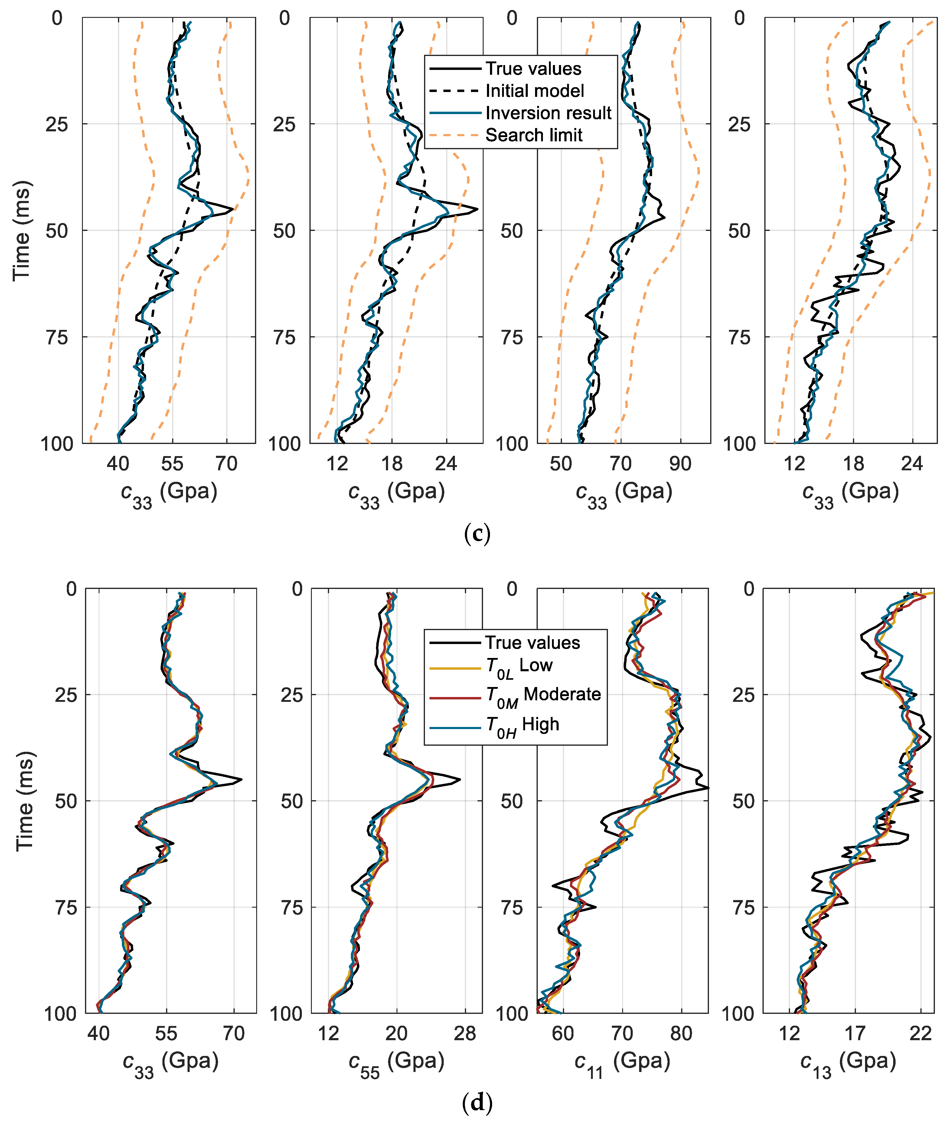
3.1. Initial Temperature

Test 1: In analyzing the influence of initial temperature, all the other optimization parameters are fixed, including the initial model, perturbation range, regularization weight, search limit, and the number of iterations. Three initial temperatures are analyzed, i.e., a high temperature (T_0H = 2.62), a moderate one (T_0M = 0.131), and a low one (T_0L = 0.00262). The initial model of five parameters is given with black dash curve and the search limit is designed based on the initial model with the orange dash curve in Figure 4a. The perturbation range is set as Δm_PA = [Δc₃₃, Δc₅₅, Δc₁₁, Δc₁₃, Δρ] = [0.111 Gpa, 0.170 Gpa, 0.241 Gpa, 0.101 Gpa, 0.0073 g/cm³]. Figure 4a–c shows the inversion results obtained by the FSA optimization approach with the low, moderate, and high initial temperatures, respectively. To demonstrate the effect of initial temperature on the convergence rate and result, the convergence curves are given describing the misfit (objective function) evolution for the three optimization procedures in Figure 5. It is shown that the initial temperature exhibits apparent effects on the inversion result, which vary with the different target parameters. The results of stiffness parameters c₁₁ and c₁₃ are more sensitive to the temperature. Compared with the high and low temperatures, the moderate one (Figure 4b) yields the best result, which can be observed from the estimations of c₅₅, c₁₁, and c₁₃ in Figure 4d. Notably, the low temperature typically suffers from immature convergence. Although the high initial temperature (blue curve in Figure 5) increases the convergence rate, it causes more fluctuations at the early stage and fails to obtain a reasonable estimation. Therefore, proper setting of initial temperature improves the convergence performance as well as the final result.

3.2. Perturbation Range

Test 2: To analyze the influences of perturbation ranges on the result, four inversions are performed by using different perturbation ranges. Similarly, the other optimization parameters are fixed. The initial model, regularization weight, search limit, and the number of iterations are the same as those of Test 1. The initial temperature is set as 0.5, which corresponds to the moderate temperature according to previous analysis, and the initial model and search limit are given as black and orange dash curves in Figure 6a–d, respectively. The four perturbation range vectors are

$$\begin{array}{cc}\Delta m_{PA1}& =\left[\Delta c_{331},\Delta c_{551},\Delta c_{111},\Delta c_{131},\Delta {\rho }_1\right]\hfill \\ & =\left[0.043\mathrm{Gpa},0.051\mathrm{Gpa},0.072\mathrm{Gpa},0.029\mathrm{Gpa},0.0022{\mathrm{g}/\mathrm{cm}}^3\right],\end{array}$$

$$\begin{array}{cc}\Delta m_{PA2}& =\left[\Delta c_{332},\Delta c_{552},\Delta c_{112},\Delta c_{132},\Delta {\rho }_2\right]\hfill \\ & =\left[0.112\mathrm{Gpa},0.135\mathrm{Gpa},0.192\mathrm{Gpa},0.077\mathrm{Gpa},0.0058{\mathrm{g}/\mathrm{cm}}^3\right],\end{array}$$

$$\begin{array}{cc}\Delta m_{PA3}& =\left[\Delta c_{333},\Delta c_{553},\Delta c_{113},\Delta c_{133},\Delta {\rho }_3\right]\hfill \\ & =\left[0.166\mathrm{Gpa},0.187\mathrm{Gpa},0.265\mathrm{Gpa},0.106\mathrm{Gpa},0.0087{\mathrm{g}/\mathrm{cm}}^3\right],\end{array}$$

$$\begin{array}{cc}\Delta m_{PA4}& =\left[\Delta c_{334},\Delta c_{554},\Delta c_{114},\Delta c_{134},\Delta {\rho }_4\right]\hfill \\ & =\left[0.334\mathrm{Gpa},0.424\mathrm{Gpa},0.580\mathrm{Gpa},0.233\mathrm{Gpa},0.018{\mathrm{g}/\mathrm{cm}}^3\right],\end{array}$$

The ranges gradually increase from $\Delta m_{PA1}$ to $\Delta m_{PA2}$, by which four sets of the inversion results are obtained with the conventional FSA and shown in Figure 6a–d. The influence of perturbation range on inversion can be observed with the comparisons of inverted results (Figure 6e) and convergence curves (Figure 7). It is shown that (a) similar to the initial temperature, the perturbation range has more significant effects on c₁₁ and c₁₃ among the four stiffness parameters; (b) a small range may lead to an immature convergence of the optimization procedure and fail to obtain an acceptable result; (c) with the increase of ranges, the convergence speed generally increases and the final misfit decreases (see Δm_PA1 to Δm_PA3 in Figure 7); (d) the moderate range Δm_PA3 yields the best inversion result; (e) the overlarge range Δm_PA4 leads to an unstable inversion result (gray curve in Figure 6e) with more errors (greater misfit). In setting a perturbation range, an adaptive method may be essential to provide a suitable and moderate one.

3.3. Search Limit

Test 3: Since the search limit is generated according to the initial model, the four search limits are considered to analyze the effects on the FSA inversion, which are modified based on the smoothing initial models. We obtain two smoothing initial models by changing the smoothing parameter SP (the span of the moving average filter), namely, the initial model 1 with SP = 25 and the initial model 2 with SP = 15. Smaller SP better describes the true model. A scale factor is applied on the initial model, and a small, moderate, or large limit is obtained depending on the factor. The search limits are given as limit 1 (orange dash curve in Figure 8a), and a small limit generated with the initial model 1 (black dash curve); limit 2 (orange dash curve in Figure 8b), and a moderate limit with the initial model 1; limit 3 (orange dash curve in Figure 8c), and a large limit with the initial model 1; limit 4 (orange dash curve in Figure 8d), a moderate limit with the initial model 2 (black dash curve in Figure 8d). The other optimization parameters are fixed, the initial temperature is set as 0.5, and the perturbation range vector and number of iterations are the same as Test 1. Figure 8a–d shows the inversion results with the limits 1–4, respectively, and the comparison of these results are given in Figure 8e. To quantify the optimization processes, the corresponding convergence curves are shown in Figure 9. By using the initial model 1, the result with the small limit is unacceptable, especially for the case when it starts from the initial model with an apparent difference from the true model (yellow curve in Figure 8e). The convergence speed improves and the final misfit (error) reduces when the limit is extended to a moderate one (red curve in Figure 9). With a successive increase of the limit, the misfit slightly increases (blue curve in Figure 9), indicating that the large limit is not essentially needed. Limit 4 yields the best result with the lowest error, which can be observed from the gray curve in both Figure 8e and Figure 9. The search limit has a significant influence on the FSA inversion. A suitable limit generated from an appropriate initial model could be much more helpful.

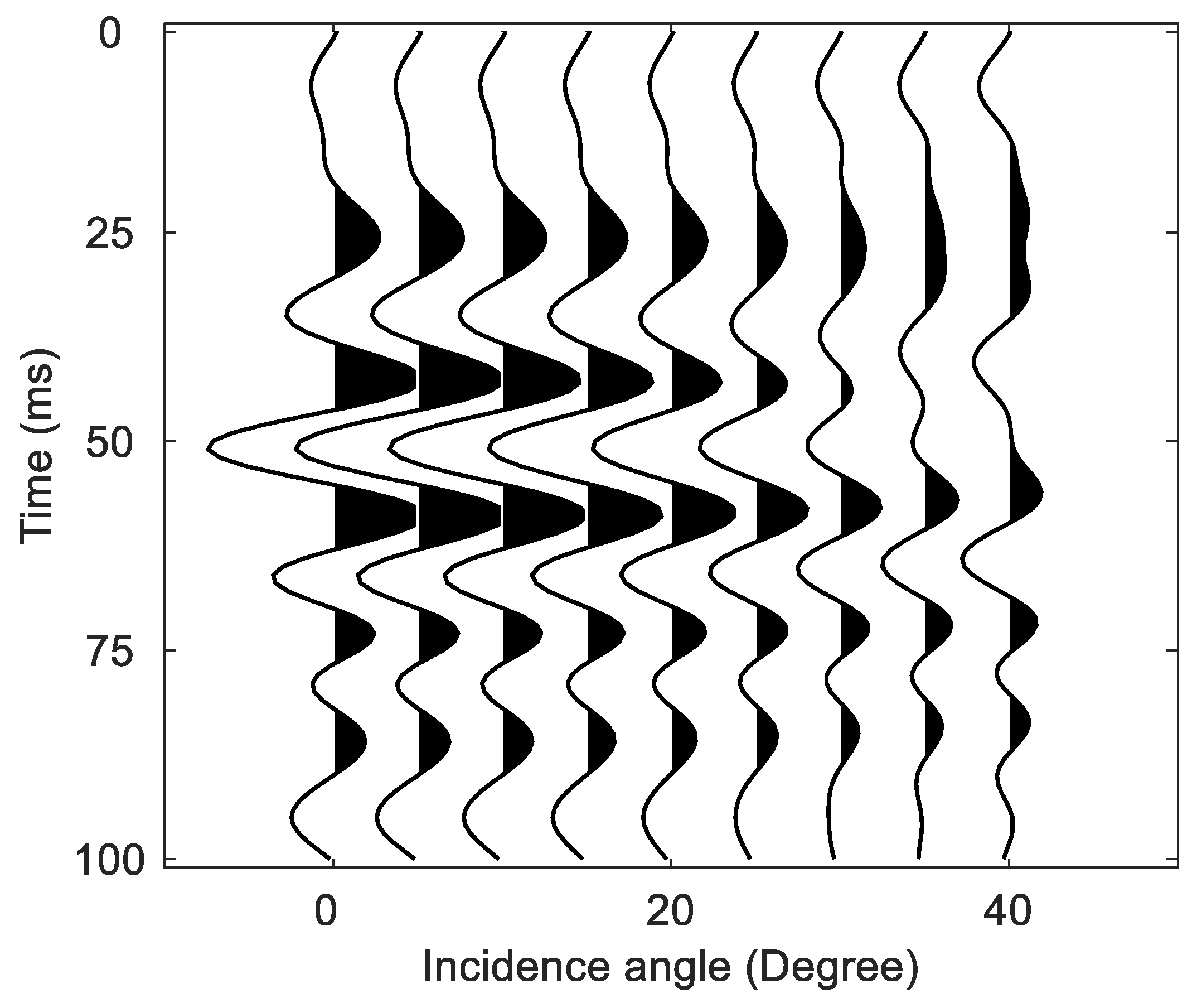
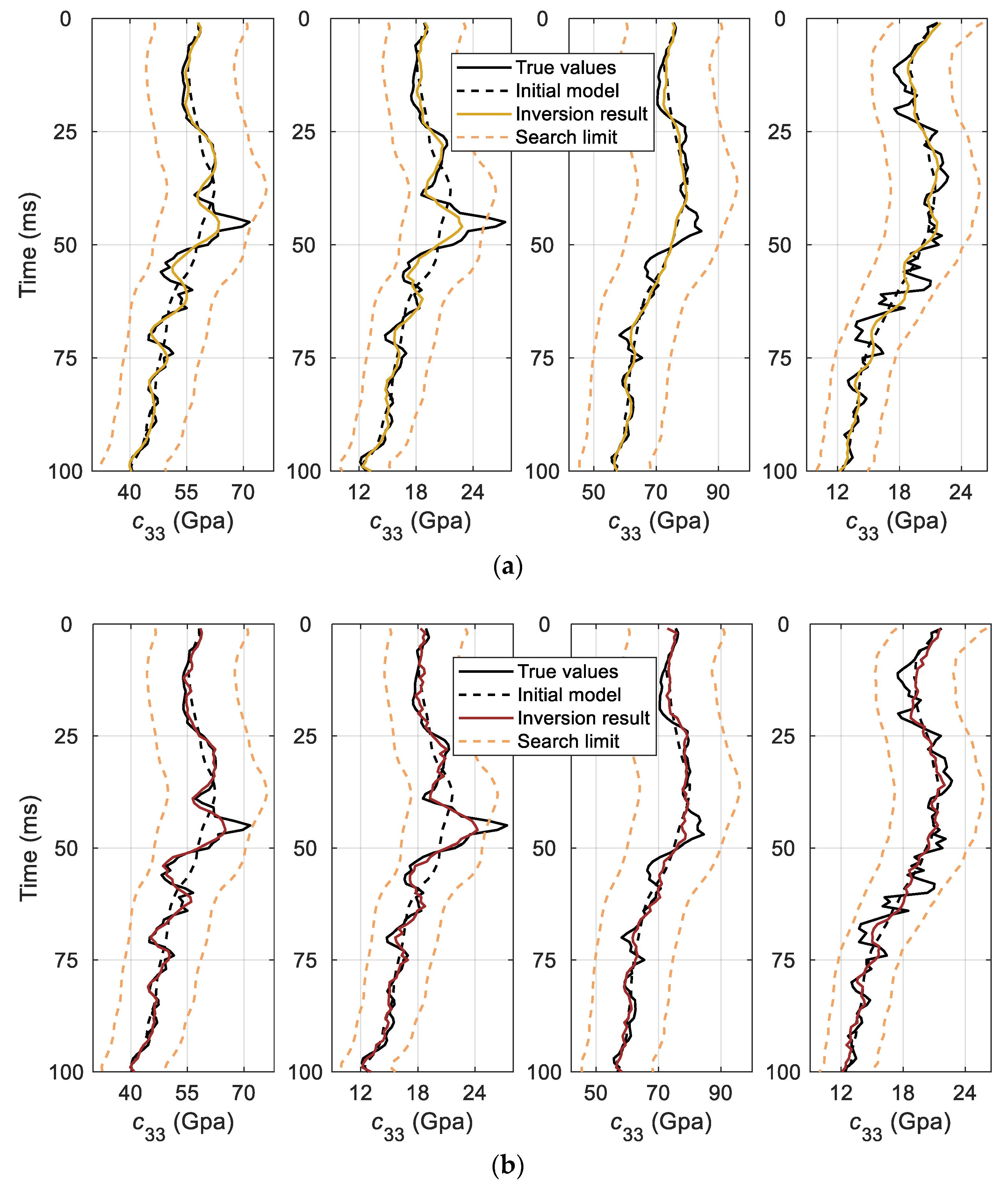
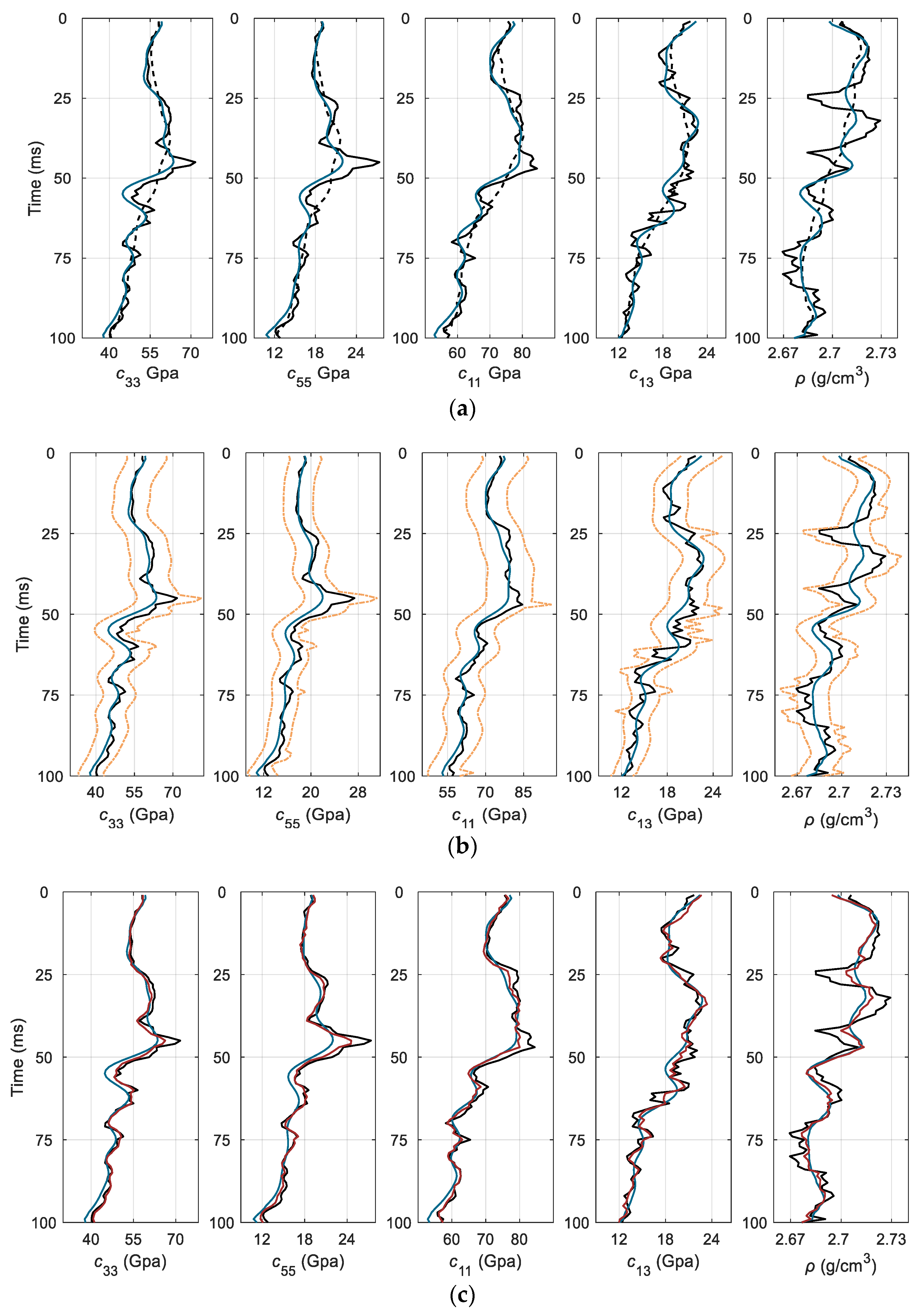
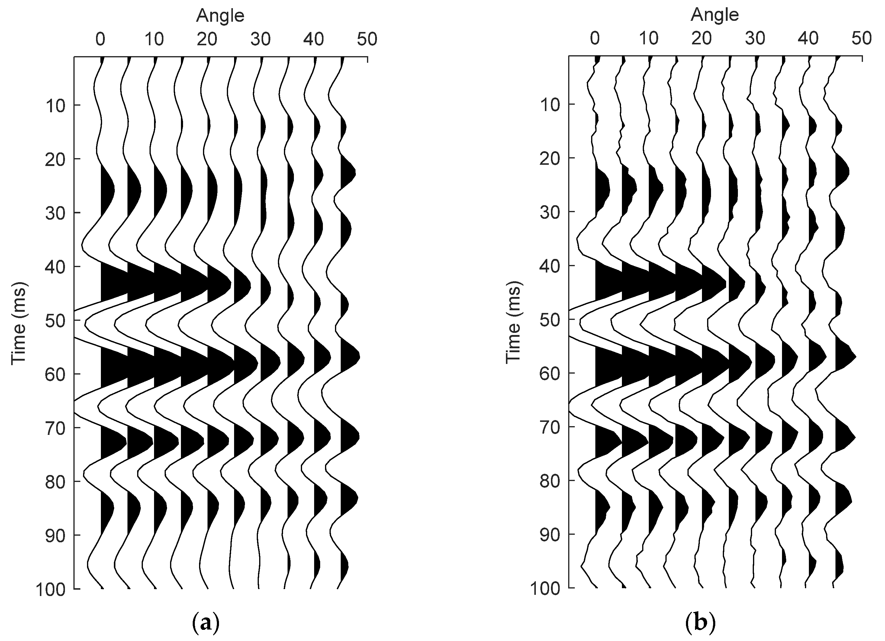
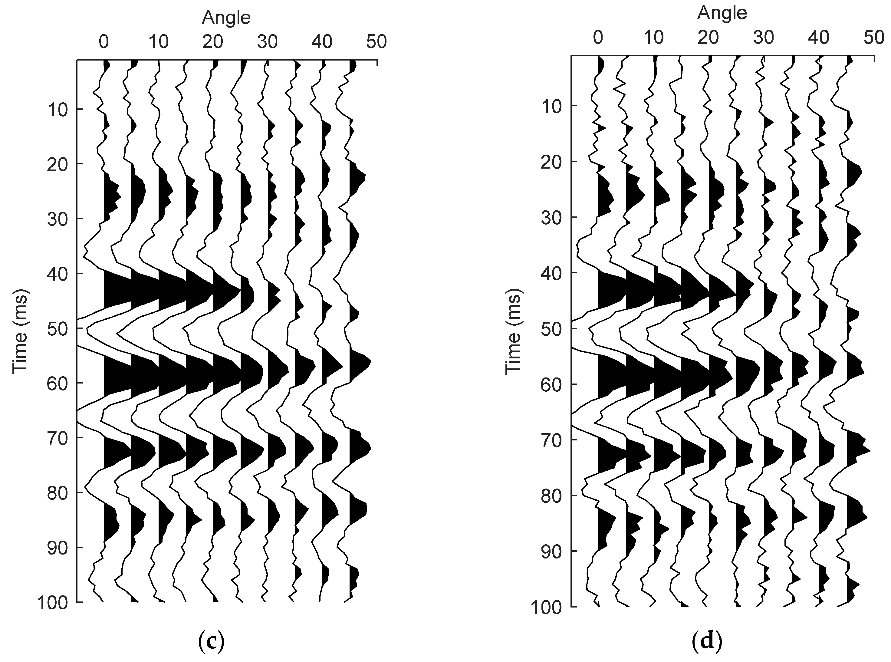
4. Synthetic Data Test

The well log model in Figure 2 is further considered to verify the proposed method by using the synthetic input gather as shown in Figure 3. In this section, three inversions are compared, i.e., Test 4 of the commonly used linear inversion based on the Rüger approximation (the linear step of the sequential method), Test 5 of the nonlinear inversion based on the Graebner exact reflection coefficient by using the FSA method with the adaptive optimization parameter setting aided by the linear result (the nonlinear step of the sequential method), and Test 6 of the full nonlinear inversion based on the Graebner exact reflection coefficient by using the conventional FSA without the aid of the linear result. The damping coefficient is set as 0.95 and the maximum iteration is set as 20,000 in the tests. However, to improve the inversion efficiency, the iteration process will be terminated if twenty consecutive perturbations are rejected.

In Test 4, we first obtain the inversion results of the parameters v_P, v_S, ρ, ε, and δ, and then compute the estimations of c₃₃, c₅₅, c₁₁, c₁₃, and ρ according to Equation (12), which are the outputs of the linear step of the sequential method. In Test 5, we set up the initial model, and we compute the prior term and estimate the optimization parameters (including the initial temperature, perturbation range, and search limit) aided by the linear result of Test 4, followed by the FSA nonlinear inversion. The preliminary (Test 4) and final results (Test 5) of the proposed method are shown as the blue curve in Figure 10a and the red curve in Figure 10c, respectively. The black solid and black dash curves are the true logs and the initial model for the linear inversion (Test 4), respectively. The orange dash curve in Figure 10b shows the search limit generated from the linear result. We compute the correlation coefficients between the true model and the results of the Rüger linear inversion (the commonly used method and the linear step of the sequential scheme) and the FSA aided by the linear results (the nonlinear step of the sequential scheme), respectively, as is shown in

Table 1. Correlation coefficients of the inversion results in Figure 10a,c and the true models.

Correlation Coefficients	c33	c55	c11	c13	ρ
Rüger inversion (linear step)	0.9605	0.9413	0.9324	0.9102	0.8731
Aided FSA (nonlinear step)	0.9932	0.9825	0.9801	0.9717	0.9201

. Figure 10 indicates that although the linear result of Test 4 contains anomalies (see Table 1), they are close to the true values compared with the provided initial models (see the black dash curve). The setting method of search limit (Equations (16) and (17)) considers all feasible solution spaces as well as reduces the searching window. The FSA approach yields a significant improvement of inversion result, especially for the anisotropy-related stiffnesses c₁₁ and c₁₃ and density ρ, when it is constrained by the linear result and the adaptive parameter settings are incorporated. The improvement can be quantified with the corresponding correlation coefficients, i.e., 0.9932 (c₃₃), 0.9825 (c₅₅), 0.9801 (c₁₁), 0.9717 (c₁₃), and 0.9201 (ρ).

Test 6 adopts the conventional FSA, which is not constrained by the linear result. The initial temperature and perturbation range vector are the same as Test 3. The search limit (orange dash curve in Figure 11a) is obtained by the constrains of the provided initial model (black dash curve in Figure 11a). Figure 11b shows the comparison of the results of Test 5 (red) and Test 6 (gray).

Table 2. Correlation coefficients of the inversion results in Figure 11a and the true models.

Correlation Coefficients	c33	c55	c11	c13	ρ
Conventional FSA	0.9806	0.9719	0.9626	0.9495	0.8737

shows the correlation coefficients between the result of the conventional FSA (gray curves in Figure 11a) and the true model. The sequential method with an adaptive parameter setting (Test 5) yields a better result than the conventional FSA (Test 6), especially for c₁₁, c₁₃, and ρ, where the lower correlation coefficients of the result of Test 6 are obtained (see Table 2). Since the anisotropic inversion for VTI media is concerned with the anisotropy-related parameters c₁₁ and c₁₃, the proposed method with adaptive FSA is helpful in inverting the anisotropy information.

Although the proposed method improves the results of the five parameters, it is also shown that the results of c₁₃ and ρ exhibit lower accuracy compared to those of c₃₃, c₅₅, and c₁₁. There is a highly coupled relation between density and the four stiff parameters according to Equation (12), which causes the unacceptable density. To overcome this problem, the parameterization of the objective function should be improved by decoupling density with the other parameters. To obtain a better result of c₁₃, a joint inversion with PP and PS data may be considered.

To further evaluate the proposed method, we analyze the inversion result from seismic data with different noise levels in terms of signal-to-noise ratios (SNRs) in Test 7. The Gaussian random noise is added to the synthetic gather (Figure 12a) to obtain the new input data, as shown in Figure 12b–d, which correspond to the noisy gathers with SNRs of 10, 5, and 3, respectively. The noise may be caused by forward modeling or observation errors. The inversion results are shown in Figure 13 with the accuracy in terms of correlation coefficient listed in

Table 3. Correlation coefficients of the inversion results in Figure 13a–c and the true models.

Correlation Coefficients	c33	c55	c11	c13	ρ
SNR = 10	0.9846	0.9731	0.9703	0.9598	0.8889
SNR = 5	0.9808	0.9681	0.9611	0.9543	0.8769
SNR = 3	0.9744	0.9630	0.9587	0.9501	0.8643

. Although the density result exhibits the lowest accuracy in those tests, its accuracy exhibits a reduction of 5% as the SNR of seismic data declines from 10 dB to 3 dB (and a reduction of 8% from noise free to noise level of 3 dB). The test indicates the proposed method has a satisfactory anti-noise performance with the adopted global optimization.

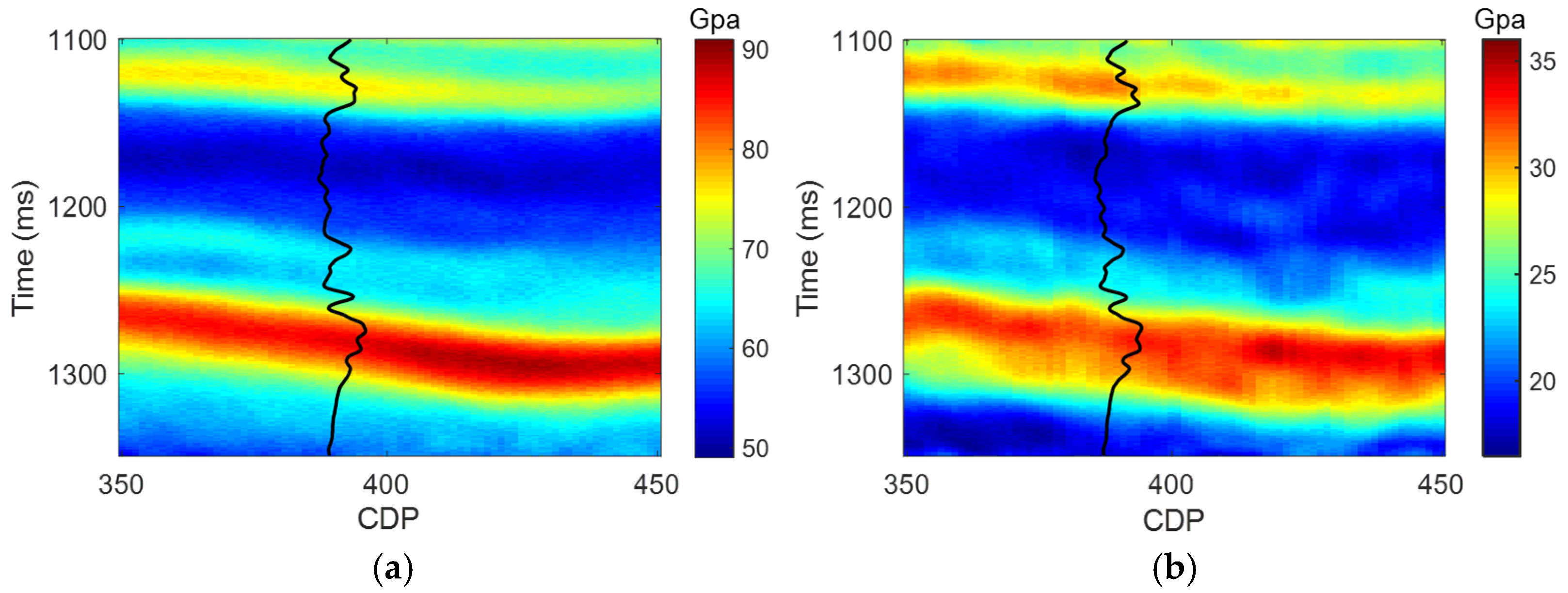
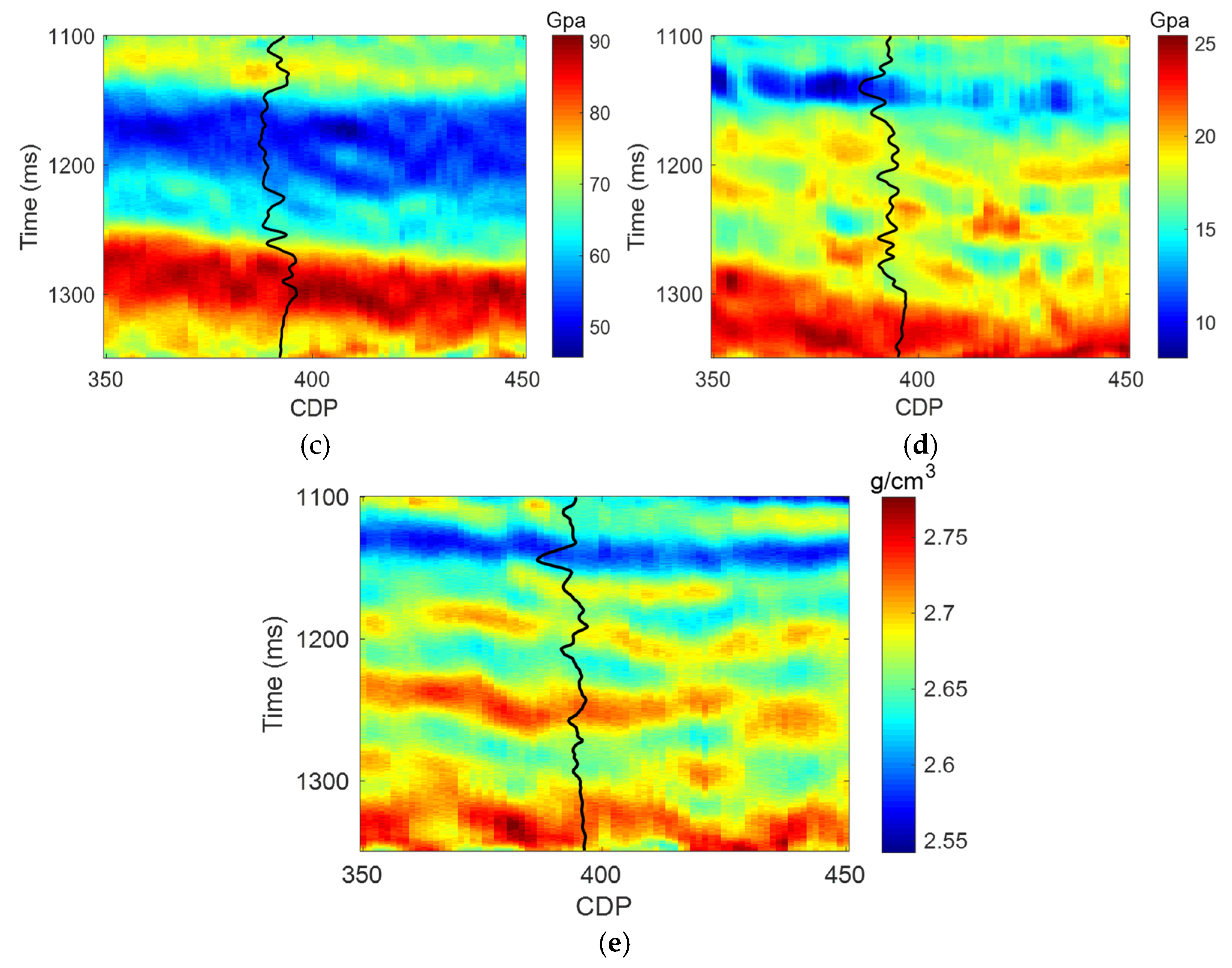
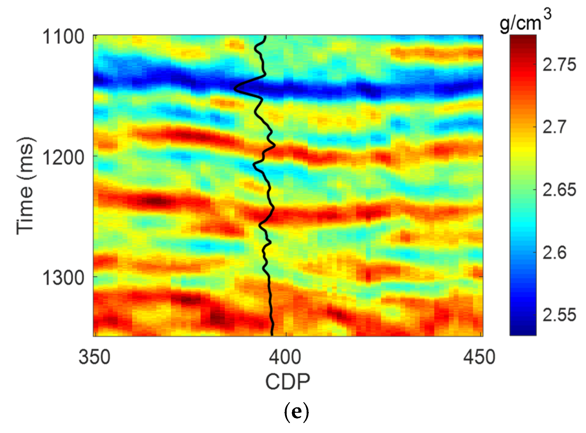
5. Real Data Application

A real seismic dataset is considered to verify the proposed method. The seismic data is acquired from a gas-bearing shale reservoir survey of Sichuan Basin, southwest China. The log data of a well for the target layers are shown in Figure 14, including the four elastic stiffness parameters of c₃₃, c₅₅, c₁₁, and c₁₃, and density ρ. The input data are seismic angle gathers. Each gather ranges from 5 to 45 degrees. Five partially stacked seismic profiles are obtained by processing the angle gathers corresponding to the constant angle sections of 9, 17, 25, 33, and 41 degrees. The angle-dependent source wavelets for the inversion are extracted from these data using the statistical method [45].

We first perform the Rüger approximation based linear inversion to obtain the preliminary result. The initial model used for the linear inversion is built by interpolating logs along the interpreted geological horizons. The linear inversion result is shown in Figure 15, and is overlapped by the relevant log curves at the well location. We set the linear result as the initial model for the subsequent FSA inversion. The optimization parameters of FSA are set according to the linear result, where the initial temperature, search limit, and perturbation range are estimated trace by trace according to Equations (14)–(18). The estimation aided by the linear result enables an adaptive optimization setting according to the data of each seismic gather. The prior term is computed based on the linear result so as to provide a reliable constraint for the nonlinear inversion. Figure 16a–e shows the final results of the five parameters using the proposed method. Compared to the linear result, the final results reveal more structural details with better lateral continuity. In order to evaluate the two sets of results, we compute the correlation coefficients between the true logs and the results at the well location (

Table 4. Correlation coefficients of the inversion results by seismic traces near the well in Figure 13 and Figure 14 and the real logs.

Correlation Coefficients	c33	c55	c11	c13	ρ
Rüger inversion (linear step)	0.818	0.767	0.726	0.631	0.627
Aided FSA (nonlinear step)	0.875	0.841	0.819	0.721	0.715

). From this it is revealed that, compared to the linear result, the sequential inversion result shows a better consistency with the log data.

6. Discussion

The proposed method is motivated by the significance of setting optimization parameters in the simulated annealing algorithm, especially for complex reservoirs involved with the observation variations among different seismic traces in a VTI inversion. We hereby propose the sequential inversion method, wherein the simulated annealing nonlinear inversion is driven by a Bayesian linear inversion. In particular, the linear result not only provides reliable prior constraints, but also enables an adaptive setting of the optimization parameters for the simulated annealing inversion.

The simulated annealing endows better capability of escaping local minima for the multi-modal and multi-parameter inverse problems. Furthermore, the proposed method does not require considerable extra computational cost, since the linear inversion and optimization parameter estimation take much less time compared with the simulated annealing inversion process, which enables us to select the global optimization of simulated annealing for solving the seismic VTI inversion problem. Admittedly, other nonlinear or probabilistic inversion methods can also be employed; however, this work focuses on addressing the observation variations among different seismic traces for complex reservoirs rather than delving into the algorithm itself. The efforts that we have made (the two-step inversion strategy) not only improve the accuracy of optimization parameters, but also provide reliable prior models to constrain the inversion process, which make the proposed method a broad applicability.

The test indicates that twenty thousand iterations are required to guarantee convergence. In practice, the optimization process is terminated if twenty consecutive perturbations are rejected, by which the total iteration number can be largely reduced. However, the computational cost should be considered when applying to large-scale 3D surveys. Future studies are supposed to make efforts on improving the computational efficiency for the method.

7. Conclusions

In this work, we propose a sequential inversion method for VTI media by using the FSA approach with adaptive setting of the optimization parameters. The method adaptively estimates the optimization parameters (i.e., initial temperature, perturbation limit, and search range) of FSA aided by the linear inversion result, which effectively improves the final results. Since forward modeling is a key factor of inversion procedure, the exact reflection coefficient of VTI media proposed by Graebner is employed to improve the accuracy of the method. The proposed method is tested on both synthetic and real seismic data, which demonstrates the advantage over the conventional FSA inversion. The method obtains the results with improved accuracy and stability, especially for c₁₁ and c₁₃. Whereas, further improvement can be achieved on density and c₁₃ by decoupling density with the other parameters and employing a joint PP- and PS-wave inversion scheme.

References

1. Chen, H. Seismic frequency component inversion for elastic parameters and maximum inverse quality factor driven by attenuating rock physics models. Surv. Geophys. 2020, 41, 835–857. [Google Scholar] [CrossRef]
2. Huang, G.; Ba, J.; Gei, D.; Carcione, J. A matrix-fracture-fluid decoupled PP reflection coefficient approximation for seismic inversion in tilted transversely isotropic media. Geophysics 2022, 87, M275. [Google Scholar] [CrossRef]
3. Huang, G.; Chen, X.; Luo, C.; Chen, Y. Mesoscopic wave-induced fluid flow effect extraction by using frequency-dependent prestack waveform inversion. IEEE Trans. Geosci. Remote Sens. 2021, 59, 6510–6524. [Google Scholar] [CrossRef]
4. Luo, C.; Huang, G.; Chen, X.; Chen, Y. Registration free multicomponent joint AVA inversion using optimal transport. IEEE Trans. Geosci. Remote Sens. 2022, 60, 4501513. [Google Scholar] [CrossRef]
5. Luo, C.; Ba, J.; Huang, G.; Carcione, J. A Born-WKBJ pre-stack seismic inversion based on a 3-D structural-geology model building. IEEE Trans. Geosci. Remote Sens. 2022, 60, 4505011. [Google Scholar] [CrossRef]
6. Zong, Z.; Sun, Q. Density stability estimation method from pre-stack seismic data. J. Pet. Sci. Eng. 2022, 208, 109373. [Google Scholar] [CrossRef]
7. Zong, Z.; Li, K.; Yin, X.; Zhu, M.; Du, J.; Chen, W.; Zhang, W. Broadband seismic amplitude variation with offset inversion. Geophysics 2017, 82, M43–M53. [Google Scholar] [CrossRef]
8. Chen, H.; Han, J.; Geng, J.; Innanen, K. Anisotropic anelastic impedance inversion for attenuation factor and weaknesses combining Newton and Bayesian Markov chain Monte Carlo algorithms. Surv. Geophys. 2022, 43, 1845–1872. [Google Scholar] [CrossRef]
9. Guo, Q.; Ba, J.; Luo, C.; Pang, M. Seismic rock physics inversion with varying pore aspect ratio in tight sandstone reservoirs. J. Pet. Sci. Eng. 2021, 207, 109131. [Google Scholar] [CrossRef]
10. Guo, Q.; Ba, J.; Carcione, J. Multi-objective petrophysical seismic inversion based on the double-porosity Biot-Rayleigh model. Surv. Geophys. 2022, 43, 1117–1141. [Google Scholar] [CrossRef]
11. Guo, Q.; Ba, J.; Luo, C. Nonlinear petrophysical AVO inversion inversion with spatially-variable pore aspect ratio. Geophysics 2022, 87, M111–M125. [Google Scholar] [CrossRef]
12. Guo, Z.; Zhao, D.; Liu, C. A new seismic inversion scheme using fluid dispersion attribute for direct gas identifification in tight sandstone reservoirs. Remote Sens. 2022, 14, 5326. [Google Scholar] [CrossRef]
13. Li, K.; Yin, X.; Zong, Z.; Grana, D. Estimation of porosity, fluid bulk modulus, and stiff-pore volume fraction using a multi-trace Bayesian AVO petrophysics inversion in multi-porosity reservoirs. Geophysics 2021, 87, 1–101. [Google Scholar] [CrossRef]
14. Zong, Z.; Yin, X.; Wu, G. Geofluid discrimination incorporating poroelasticity and seismic reflection inversion. Surv. Geophys. 2015, 36, 659–681. [Google Scholar] [CrossRef]
15. Ding, P.; Gong, F.; Zhang, F.; Li, X. A physical model study of shale seismic responses and anisotropic inversion. Pet. Sci. 2021, 18, 1059–1068. [Google Scholar] [CrossRef]
16. Sayers, C.; den Boer, L. Shale anisotropy and the elastic anisotropy of clay minerals. In SEG Technical Program Expanded Abstracts 2014; Society of Exploration Geophysicists: Houston, TX, USA, 2014; pp. 2829–2833. [Google Scholar]
17. Wright, J. The effects of transverse isotropy on reflection amplitudes versus offset. Geophysics 1987, 52, 564–567. [Google Scholar] [CrossRef]
18. Wang, L.; Zhang, F.; Li, X.; Di, B.; Zeng, L. Quantitative seismic interpretation of rock brittleness based on statistical rock physics. Geophysics 2019, 84, IM63–IM75. [Google Scholar] [CrossRef]
19. Carcione, J.; Avseth, P. Rock-physics templates for clay-rich source rocks. Geophysics 2015, 80, D481–D500. [Google Scholar] [CrossRef]
20. Ba, J.; Xu, W.; Fu, L.; Carcione, J.; Zhang, L. Rock anelasticity due to patchy saturation and fabric heterogeneity: A double doubleporosity model of wave propagation. J. Geophys. Res.-Solid Earth 2017, 122, 1949–1976. [Google Scholar] [CrossRef]
21. Carcione, J. Reflflection and transmission of qP-qS plane waves at a plane boundary between viscoelastic transversely isotropic media. Geophys. J. Int. 1997, 129, 669–680. [Google Scholar] [CrossRef]
22. Graebner, M. Plane-wave reflflection and transmission coeffificients for a transversely isotropic solid. Geophysics 1992, 57, 1512–1519. [Google Scholar] [CrossRef]
23. Schoenberg, M.; Protazio, J. ‘Zoeppritz’ rationalized and generalized to anisotropy. J. Seism. Explor. 1992, 1, 125–144. [Google Scholar]
24. Thomsen, L. Weak elastic anisotropy. Geophysics 1986, 51, 1954–1966. [Google Scholar] [CrossRef]
25. Rüger, A. P-wave reflflection coeffificients for transversely isotropic models with vertical and horizontal axis of symmetry. Geophysics 1997, 62, 713–722. [Google Scholar] [CrossRef]
26. Rüger, A. Variation of P-wave reflectivity with offset and azimuth in anisotropic media. Geophysics 1998, 63, 935–947. [Google Scholar] [CrossRef]
27. Lu, J.; Wang, Y.; Chen, J.; An, Y. Joint anisotropic amplitude variation with offset inversion of PP and PS seismic data. Geophysics 2018, 83, N31–N50. [Google Scholar] [CrossRef]
28. Plessix, R.; Bork, P. Quantitative estimate of VTI parameters from AVA responses. Geophys. Prospect. 2000, 48, 87–108. [Google Scholar] [CrossRef]
29. Zhang, F.; Zhang, T.; Li, X. Seismic amplitude inversion for the transversely isotropic media with vertical axis of symmetry. Geophys. Prospect. 2019, 67, 2368–2385. [Google Scholar] [CrossRef]
30. Zhang, F.; Wang, L.; Li, X. Characterization of a shale-gas reservoir based on a seismic AVO inversion for VTI media and quantitative seismic interpretation. Interpretation 2020, 8, SA11. [Google Scholar] [CrossRef]
31. Luo, C.; Ba, J.; Carcione, J.; Huang, G.; Guo, Q. Joint PP and PS pre-stack AVA inversion for VTI medium based on the exact Graebner equation. J. Pet. Sci. Eng. 2020, 194, 107416. [Google Scholar] [CrossRef]
32. Luo, C.; Ba, J.; Carcione, J. A Hierarchical Prestack Seismic Inversion Scheme for VTI Media Based on the Exact Reflection Coefficient. IEEE Trans. Geosci. Remote Sens. 2022, 60, 4507416. [Google Scholar] [CrossRef]
33. Guo, Q.; Ba, J.; Luo, C. Prestack seismic inversion with data-driven MRF-based regularization. IEEE Trans. Geosci. Remote Sens. 2021, 59, 7122–7136. [Google Scholar] [CrossRef]
34. Ingber, L. Very fast simulated re-annealing. Math. Comput. Model. 1989, 12, 967–973. [Google Scholar] [CrossRef]
35. Sen, M.; Stoffa, P. Nonlinear one-dimensional seismic waveform inversion using simulated annealing. Geophysics 1991, 56, 1624–1638. [Google Scholar] [CrossRef]
36. Rothman, R. Nonlinear inversion, statistical mechanics, and residual statics estimation. Geophysics 1985, 50, 2784–2796. [Google Scholar] [CrossRef]
37. Guo, Q.; Zhang, H.; Cao, H.; Wei, X.; Han, F. Hybrid seismic inversion based on mulit-order anisotropic Markov random field. IEEE Trans. Geosci. Remote Sens. 2020, 58, 407–420. [Google Scholar] [CrossRef]
38. Shen, Y.; Kiatsupaibul, S.; Zabinsky, Z.; Smith, R. An analytically derived cooling schedule for simulated annealing. J. Glob. Optim. 2007, 38, 333–365. [Google Scholar] [CrossRef]
39. Basu, A.; Frazer, L. Rapid determination of the critical temperature in simulated annealing inversion. Science 1990, 249, 1409–1412. [Google Scholar] [CrossRef]
40. Aarts, E.; Korst, J. Simulated Annealing and Boltzmann Machines; John Wiley & Sons: New York, NY, USA, 1989. [Google Scholar]
41. Buland, A.; Omre, H. Bayesian linearized AVO inversion. Geophysics 2003, 68, 185–198. [Google Scholar] [CrossRef]
42. Ryden, N.; Park, C.B. Fast simulated annealing inversion of surface waves on pavement using phase-velocity spectra. Geophysics 2007, 71, R49–R58. [Google Scholar] [CrossRef]
43. Ma, X. Simultaneous inversion of prestack seismic data for rock properties using simulated annealing. Geophysics 2002, 67, 1877–1885. [Google Scholar] [CrossRef]
44. Bianco, E. Tutorial: Wavelet estimation for well ties. Lead. Edge 2016, 35, 541–543. [Google Scholar] [CrossRef]
45. Tarantola, A. Inverse Problem Theory and Methods for Model Parameter Estimation; Society for Industrial and Applied Mathematics (SIAM): Philadelphia, PA, USA, 2005. [Google Scholar]
46. Zhi, L.X.; Chen, S.Q.; Li, X.Y. Amplitude variation with angle inversion using the exact Zoeppritz equations—Theory and methodology. Geophysics 2016, 81, N1–N15. [Google Scholar] [CrossRef]
47. Ulrych, J.T.; Sacchi, D.M.; Woodbury, A. A Bayes tour of inversion: A tutorial. Geophysics 2001, 66, 55–69. [Google Scholar] [CrossRef]
48. Rabben, E.T.; Tjelmeland, H.; Ursin, B. Non-linear Bayesian joint inversion of seismic reflection coefficients. Geophys. J. Int. 2008, 173, 265–280. [Google Scholar] [CrossRef]
49. Luo, C.; Ba, J.; Carcione, M.J.; Huang, G.T.; Guo, Q. Joint PP and PS pre-stack seismic inversion for stratifified models based on the propagator matrix forward engine. Surv. Geophys. 2020, 41, 987–1028. [Google Scholar] [CrossRef]
50. Grana, D.; Mukerji, T.; Doyen, P. Seismic Reservoir Modeling: Theory, Examples, and Algorithms; John Wiley & Sons: New York, NY, USA, 2021. [Google Scholar]
51. Luo, C.; Ba, J.; Carcione, J.; Guo, Q. Basis Pursuit Anisotropic Inversion Based on the L1-L2-Norm Regularization. IEEE Geosci. Remote Sens. Lett. 2022, 19, 8011105. [Google Scholar] [CrossRef]
Figure 1. Flowchart of the proposed sequential seismic anisotropic inversion based on the FSA algorithm with the adaptive setting of optimization parameters.
Remotesensing 15 01891 g001
Figure 2. Well model for the synthetic data test. The panels from left to right give the true values of the elastic stiffness parameters of c33, c55, c11, c13, and density ρ.
Remotesensing 15 01891 g002
Figure 3. The input synthetic seismic gather for model test generated by using the well logs of Figure 2.
Remotesensing 15 01891 g003
Figure 4. Inversion results with the well model by the FSA optimization at different initial temperatures: (a) the low temperature T0L, (b) the moderate temperature T0M, (c) the high temperature T0H, and (d) the comparison of the three sets of results from (a) to (c). The black solid, black dash, and orange dash curves are the true logs, the initial models, and the search limits, respectively. The definitions of inverted curves are given in the legend.
Remotesensing 15 01891 g004aRemotesensing 15 01891 g004b
Figure 5. Misfits varying with iteration numbers by using the different initial temperatures. The arrow shows the direction of temperature increase. The definitions of curves are given in the legend.
Remotesensing 15 01891 g005
Figure 6. Inversion results with the well model by the FSA optimization at different perturbation ranges: (a) the perturbation range ΔmPA1, (b) the perturbation range ΔmPA2, (c) the perturbation range ΔmPA3, (d) the perturbation range ΔmPA4, and (e) the comparison of the four sets of results from (a) to (d). The perturbation ranges gradually increase from ΔmPA1 to ΔmPA4. The black solid, black dash, and orange dash curves denote the true logs, the initial models, and the search limits, respectively. The definitions of inverted curves are given in the legend.
Remotesensing 15 01891 g006aRemotesensing 15 01891 g006b
Figure 7. Misfits varying with iteration number by using the different perturbation ranges. The arrow indicates the direction of range increase. The definitions of curves are given in the legend.
Remotesensing 15 01891 g007
Figure 8. Inversion results with the well model by the FSA optimization at different search limits (the orange dash curves): (a) limit 1, a small limit generated with the initial model 1, (b) limit 2, a moderate limit generated with the initial model 1, (c) limit 3, a large limit generated with the initial model 1, (d) limit 4, a moderate limit generated with the initial model 2, and (e) the comparison of four sets of inversion results from (a) to (d). The black solid, black dash, and orange dash curves are the true logs, the initial models, and search limits, respectively. The definitions of inverted curves are given in the legend.
Remotesensing 15 01891 g008aRemotesensing 15 01891 g008b
Figure 9. Misfits varying with iteration number at the different search limits. The definitions of curves are given in the legend.
Remotesensing 15 01891 g009
Figure 10. Inversion results with the well model by the proposed method. (a) The preliminary result using Rüger approximation based linear optimization (the linear step of the proposed scheme), (b) the search limit generated based on (a), and (c) the final result by the FSA with the adaptive settings of optimization parameters (the nonlinear step of the proposed scheme). The black solid, black dash, and orange dash curves are the true logs, the initial model, and the search limit, respectively. The preliminary and final inversion results are indicated by blue and red curves.
Remotesensing 15 01891 g010
Figure 11. Nonlinear inversion result with the well model by the conventional FSA without the aid of linear inversion. (a) Search limit and (b) comparison of the results by the nonlinear inversion (gray curve) and proposed method (red curve). The black solid, black dash, and orange dash curves are the true logs, the initial model, and the search limit, respectively. The red curves are same as those in Figure 10c.
Remotesensing 15 01891 g011
Figure 12. Synthetic PP seismograms computed with the exact reflection coefficient of VTI media with different SNRs by adding white Gaussian noises. (a) Noise free, (b) SNR = 10, (c) SNR = 5, and (d) SNR = 3.
Remotesensing 15 01891 g012aRemotesensing 15 01891 g012b
Figure 13. Inversion results of the proposed method by using the noisy angle gathers of Figure 12. (a) SNR = 10, (b) SNR = 5, (c) SNR = 3, and (d) the overall comparison of the inversion results of (a) to (c) and the result (red curve) in Figure 10c. The definitions of inverted curves are given in the legend.
Remotesensing 15 01891 g013aRemotesensing 15 01891 g013b
Figure 14. Well logs of the target layer. The panels from left to right give the true values of four stiffness parameters of c33, c55, c11, and c13, and density ρ.
Remotesensing 15 01891 g014
Figure 15. Inversion profiles of (a) c33, (b) c55, (c) c11, (d) c13, and (e) ρ, by using the Rüger approximation based linear optimization in the first step of the sequential method. The corresponding well logs are given.
Remotesensing 15 01891 g015aRemotesensing 15 01891 g015b
Figure 16. Final inversion profiles of (a) c33, (b) c55, (c) c11, (d) c13, and (e) ρ, by using Graebner’s exact formula and the adaptive FSA in the second step of the sequential method. The corresponding well logs are given.
Remotesensing 15 01891 g016aRemotesensing 15 01891 g016b