A Sorting Method of SAR Emitter Signal Sorting Based on Self-Supervised Clustering

Abstract

Most existing methods for sorting synthetic aperture radar (SAR) emitter signals rely on either unsupervised clustering or supervised classification methods. However, unsupervised clustering can consume a significant amount of computational and storage space and is sensitive to the setting of hyperparameters, while supervised classification requires a considerable number of labeled samples. To address these limitations, we propose a self-supervised clustering-based method for sorting SAR radiation source signals. The method uses a constructed affinity propagation-convolutional neural network (AP-CNN) to perform self-supervised clustering of a large number of unlabeled signal time-frequency images into multiple clusters in the first stage. Subsequently, it uses a self-organizing map (SOM) network combined with inter-pulse parameters for further sorting in the second stage. The simulation results demonstrate that the proposed method outperforms other depth models and conventional methods in the environment where Gaussian white noise affects the signal. The experiments conducted using measured data also show the superiority of the proposed method in this paper.

1. Introduction

Radar emitter signal sorting is a crucial aspect of modern electronic warfare, as electronic reconnaissance signals contain a vast and diverse range of information [1,2,3]. In the field of SAR electronic countermeasures, besides the traditional linear frequency modulation (LFM) waveform, SAR has started utilizing frequency-coded waveforms, phase-coded waveforms, and up-and-down chirp modulation (also known as V-shaped frequency modulation) to meet the recent demands for SAR to expand its functions and performance [4,5,6,7,8,9]. As the electromagnetic environment has become increasingly complex, detected signals often contain signals from multiple radiation sources, and there may be overlaps between the signal parameters of each radiation source. The dense pulses increase the randomness of parameter distribution, making traditional sorting methods based on single parameters (such as pulse repetition interval (PRI)) and one-dimensional sorting methods using multiple parameters step by step prone to error accumulation effects and difficulty in adapting to the complex electromagnetic environment [10,11,12]. In this sense, both subjective needs and objective realities have placed higher requirements on signal analysis work performed on received signals.

Compared with traditional sorting methods based on single parameters or step-by-step methods using multiple parameters, sorting methods based on multidimensional parameters can yield satisfactory results. Most current multidimensional parameter-based sorting methods use traditional unsupervised clustering or supervised classification methods to sort the signal based on intra-pulse and inter-pulse characteristics. Unsupervised sorting methods include K-means clustering [13], grid clustering [14], density clustering [15], hierarchical clustering [16], support vector machine classification [17], and so on. However, they are often computationally intensive or require manual assignment of parameters such as density thresholds and the number of clusters, and the initial parameter settings have a significant impact on the clustering results. Additionally, some of them can only handle a few specific signal characteristics, and some of them are sensitive to interference. In recent years, the development of digital image processing technology has provided new prospects for supervised sorting methods. By using time-frequency analysis to convert radar signals into time-frequency images and combining machine learning algorithms in computer vision, better sorting results can be obtained based on the time-frequency characteristics of the signal [18]. Tang et al. enabled the recognition of radar waveform using LRCNet, which fuses convolutional neural network (CNN) and convolutional block attention mechanism [19]. Quan et al. designed a signal sorting method that extracts the Histogram of Oriented Gradients (HOG) features and deep features from time-frequency images using a two-channel CNN and performs feature fusion with a multi-layer perceptron network [20]. However, their methods often require the manual construction of labeled datasets and can only process signals with known intra-pulse modulation types, which may not be feasible for massive pulses from noncooperative targets.

Self-supervised learning is a class of learning methods that utilize supervision available within the data to train a machine learning model. The basic idea is to use the auxiliary task to mine the unlabeled data for its distinguishable features to generate supervised information, i.e., “pseudo-labeling”, to provide supervision for downstream tasks. In the field of signal sorting and recognition, self-supervised learning can improve the utilization of massive non-cooperative signals, reduce the need for manual intervention, and maintain good classification performance.

To achieve superior sorting results, it is necessary to improve the adaptability of the signal sorting algorithm toward complex electromagnetic environments, particularly for environments containing unknown types of radiation sources. Additionally, minimizing the number of parameters that need to be set and reducing the need for manual operations will assist in streamlining the actual signal-sorting process.

Accordingly, our research proposes a SAR emitter signal-sorting method based on self-supervised clustering. The proposed method first uses a constructed affinity propagation convolutional neural network (AP-CNN) to cluster the dataset of unlabeled signal time-frequency images and then uses a SOM network in combination with inter-pulse parameters to further sorting. The anti-noise performance of the method and the classification performance for different modulation parameters and different intra-pulse modulation types are tested through simulations and proved to have better performance compared with traditional methods, such as K-nearest neighbors (KNN), support vector machines (SVM), and methods based on machine learning, such as ResNet 50 network and contrastive learning-CNN (CL-CNN). These experiments conducted using measured data also show the advantages of the proposed method in this paper.

2. Related Works

2.1. Radar Signal Sorting Methods

Conventional methods for sorting radar signals typically extract the descriptor information of individual pulses from the received waveform and rely on the individual parameter for sorting or rely on multiple parameters for deinterleaving step by step. One of the first widely used methods relies on the pulse repetition interval (PRI) for sorting [21]. Recent research explores multidimensional sorting methods combining intra- and inter-pulse parameters, macroscopic features, and fingerprint features, along with new techniques such as unsupervised clustering algorithms and supervised machine learning. Feng et al. [22] and Cao et al. [23]. proposed that K-means clustering and fuzzy C-means clustering can be used for signal sorting based on multiple parameters. Zhang et al. [24] encoded the radar pulse parameters into image form and used recurrence plots (RP), Gramian angular field (GAF), and Markov transition field (MTF) to achieve the sorting of radar signals. Li et al. [25] introduced integrated learning theory to radar signal sorting by stacking different types of deep belief networks to learn signal features in-depth and linearly integrate the posterior probabilities of each model layer before using the decision layer to determine the final classification result. Traditional machine learning-based approaches rely on expert knowledge to specify features and require significant time costs to implement. CNNs have good feature extraction capabilities, so CNN-based methods have recently been widely used for radar signal sorting and emitter recognition [26,27,28,29,30].

2.2. Self-Supervised Learning

Self-supervised learning (SSL) is a subfield of machine learning that has gained popularity in recent years as it can overcome the limitations of manually labeled samples in deep learning [31,32]. In the domain of signal sorting and recognition, self-supervised learning methods are employed to extract features from vast amounts of unlabeled samples and can be effectively trained without manual labeling, thus reducing the cost of collecting and annotating large-scale datasets [33,34]. SSL utilizes auxiliary tasks to extract useful information from the data and generate pseudo-labels to train machine-learning models. Common self-supervised learning auxiliary tasks include generative and contrastive methods.

2.3. Self-Organizing Map Network

Although the self-supervised learning method is effective at sorting pulse sequences based on time-frequency image features, it may ignore important information from the inter-pulse parameters. As a result, pulse streams with similar intra-pulse modulation types but different inter-pulse characteristics may be grouped together in the sorting results, which require further sorting. The SOM network is an unsupervised neural network that uses a competitive learning strategy to generate low-dimensional, discrete mappings by learning data in the input space [35]. SOM networks have strong generalization capabilities and can handle unlabeled input samples, which are, thereby, widely used in data compression, classification and clustering, and feature extraction [36,37,38]. The SOM networks draw on research results on the self-organizing properties of the human brain. During training, the SOM network employs a competitive learning strategy that optimizes the network gradually through neuron competition while maintaining the topology of the input space. This ensures that the adjacent samples in the input space are mapped to adjacent output neurons.

3. Signal Model and Data Preprocessing

3.1. Model of the Received Signal

SAR usually uses an LFM signal; a single LFM pulse signal can be expressed as follows:

$$x_0(t)=A\cdot rect(\frac{t}{T_p})\cdot \exp [j({\omega }_{c}t+\pi K_r{t}^2)]$$

(1)

where A is the signal amplitude, t is the time, T_p is the pulse time width, ω_c is the carrier angular frequency (initial frequency), K_r is the chirp slope, and rect(·) is the rectangular window function. In addition, in order to improve the observation performance and anti-jamming capability of SAR, some nonlinear frequency modulation techniques have been adopted, such as V-shaped FM (VFM) and orthogonal frequency division multiplexing LFM (OFDM-LFM). The VFM signal used in the research process of this paper can be expressed as follows:

$$x_0(t)=A\cdot rect(\frac{t}{T_{p0}})\cdot \exp [j({\omega }_{c}t+\pi K_r{t}^2)]+A\cdot rect(\frac{t-T_{p0}}{T_{p0}})\cdot \exp [j({\omega }_{c}t-\pi K_r{t}^2)]$$

(2)

where T_p0 is half of the pulse duration.

The OFDM-LFM signal used in this study can be expressed as follows:

$$x_0(t)=A\cdot \exp (j{\omega }_{c}t){\displaystyle \sum _{n=0}^{N-1}rect(t-n{T}_s)\cdot \exp [j{\omega }_n(t-n{T}_s)+j\pi K_r{(t-n{T}_s)}^2]}$$

(3)

where T_s is the codeword duration and ω_n is the carrier angular frequency within the codeword.

In addition, regular pulse signals are often received when acquiring signals, which can be expressed as follows:

$$x_0(t)=A\cdot rect(\frac{t}{T_p})$$

(4)

The signal received by the reconnaissance receiver is interfered with by additive Gaussian white noise to simulate the real electromagnetic environment. The received signal can be expressed as follows:

$$x(t)=x_0(t)+n(t)$$

(5)

where n(t) represents additive Gaussian white noise.

3.2. Data Preprocessing

Since self-supervised clustering methods usually require image data as input, the radar signal needs to be converted into images for pre-processing. In this paper, the smoothed pseudo-Wigner Ville distribution (SPWVD) is used to obtain the time-frequency image of each pulse as the input of AP-CNN. The SPWVD of signal x(t) is calculated as follows:

$$SPWV{D}_x(t,f)={\displaystyle {\int }_{-\infty }^{+\infty }h(\tau ){\displaystyle {\int }_{-\infty }^{+\infty }g(s-t)x(s+\frac{\tau }{2})x^{\ast }(s-\frac{\tau }{2})\exp (-j2\pi f\tau )dsd\tau }}$$

(6)

where g(·) and h(·) are the time domain window function and the frequency domain window function, respectively [39]. Since the signal may contain noise, a two-dimensional Wiener filter is used in this study to denoise the time-frequency images obtained from the SPWVD. For more details on the 2D Wiener filtering, see [40].

4. Self-Supervised Clustering Method Based on Pulse Time-Frequency Image Features

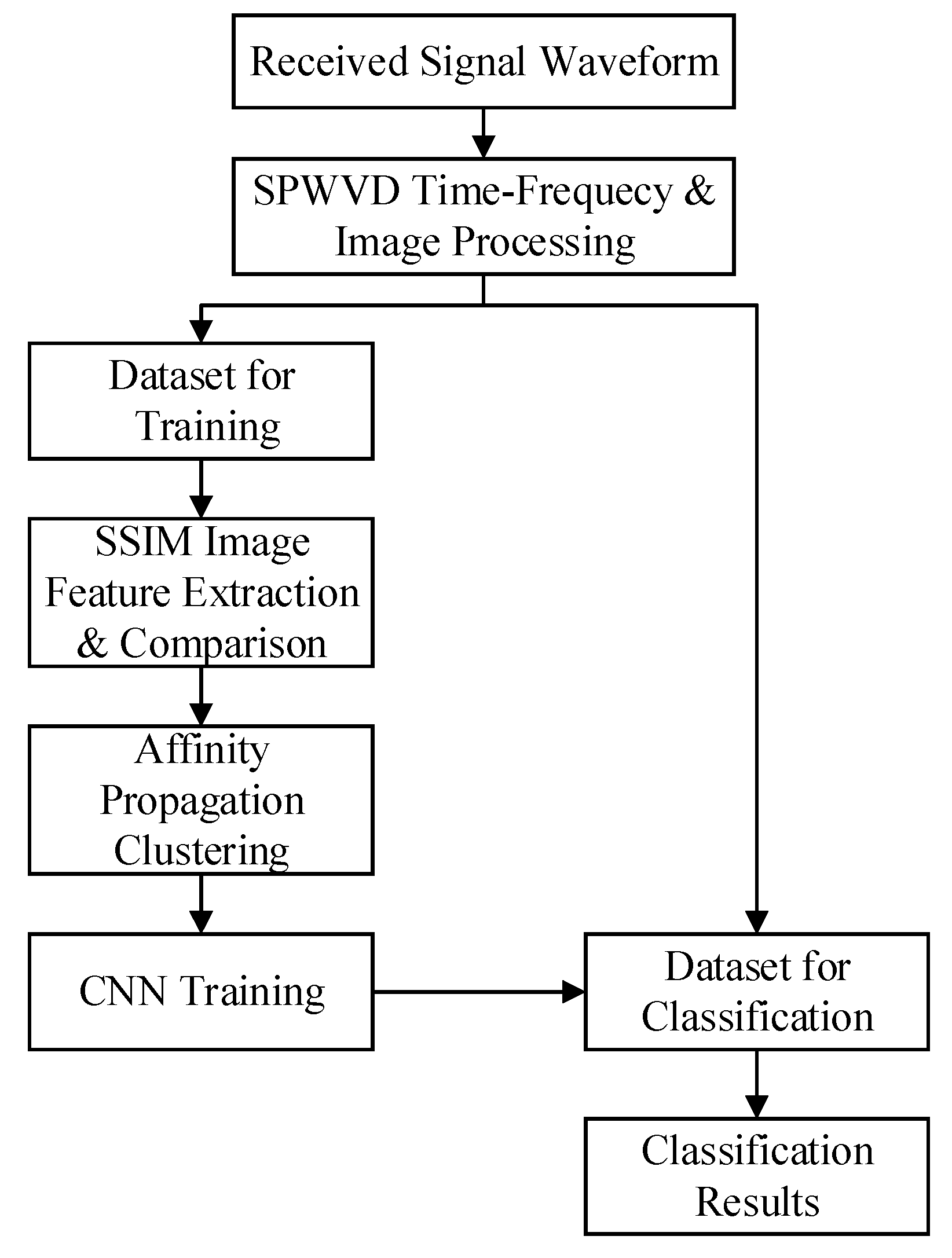
4.1. Overview of the Proposed Method

An overview of the self-supervised clustering-based sorting method designed in this paper is shown in Figure 1. First, the received signal pulses’ time-frequency images (TFI) are generated using smoothed pseudo-WVD. After that, some of the time-frequency maps are randomly selected. The structural similarity index (SSIM) is used to extract the TFI features and measure the similarity of different TFIs, and the similarity matrix is constructed accordingly. After the affinity propagation (AP) clustering of the similarity matrix, a high-quality pseudo-labeled TFI dataset is obtained, which is then used to train the CNN and realize the TFI sorting based on the intra-pulse parameters. To optimize the sorting results, we employed a SOM network that combines intra-pulse and inter-pulse features. This is because there may be pulse streams with the same intra-pulse modulation type but differing inter-pulse characteristics in the sorting results.

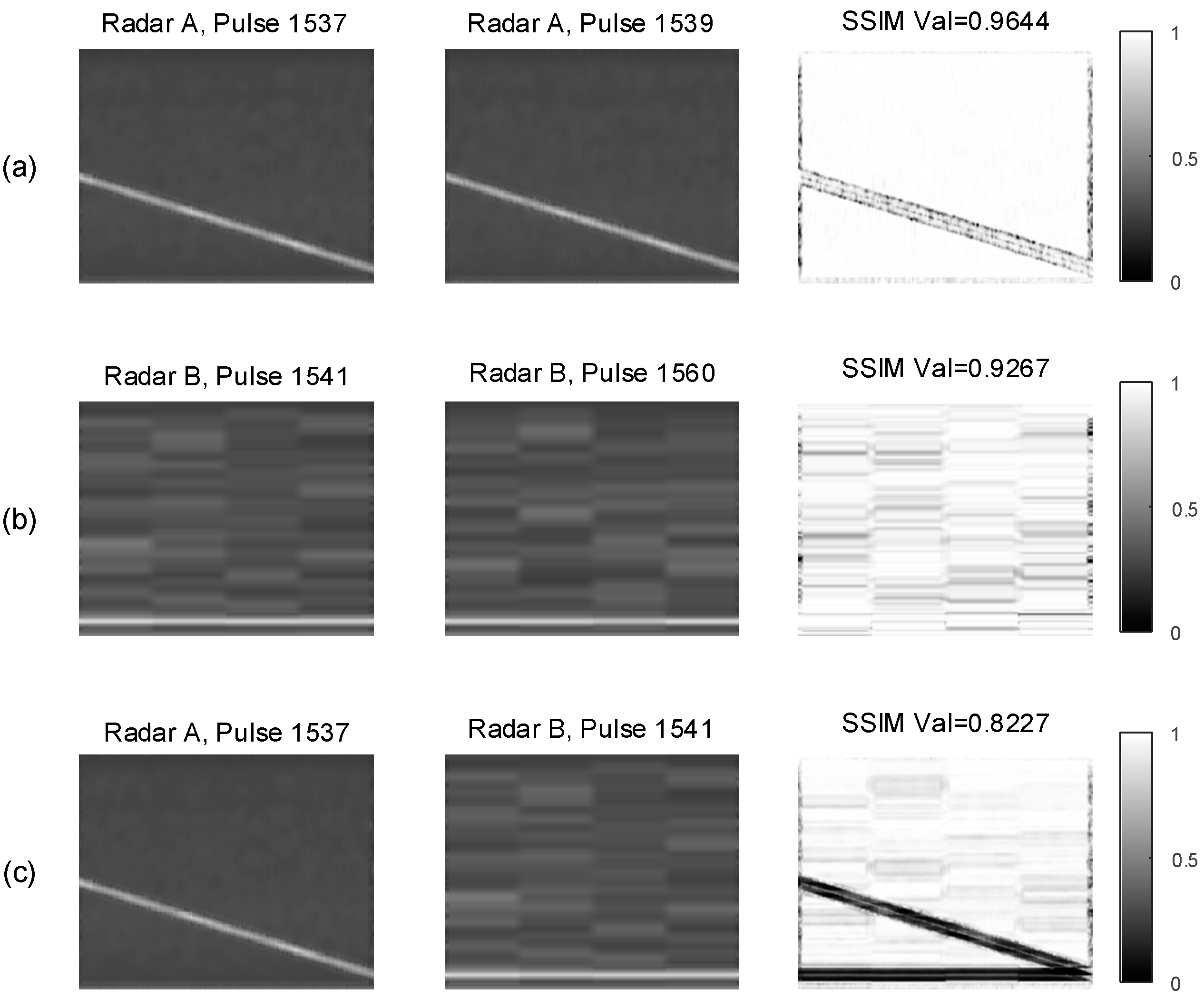
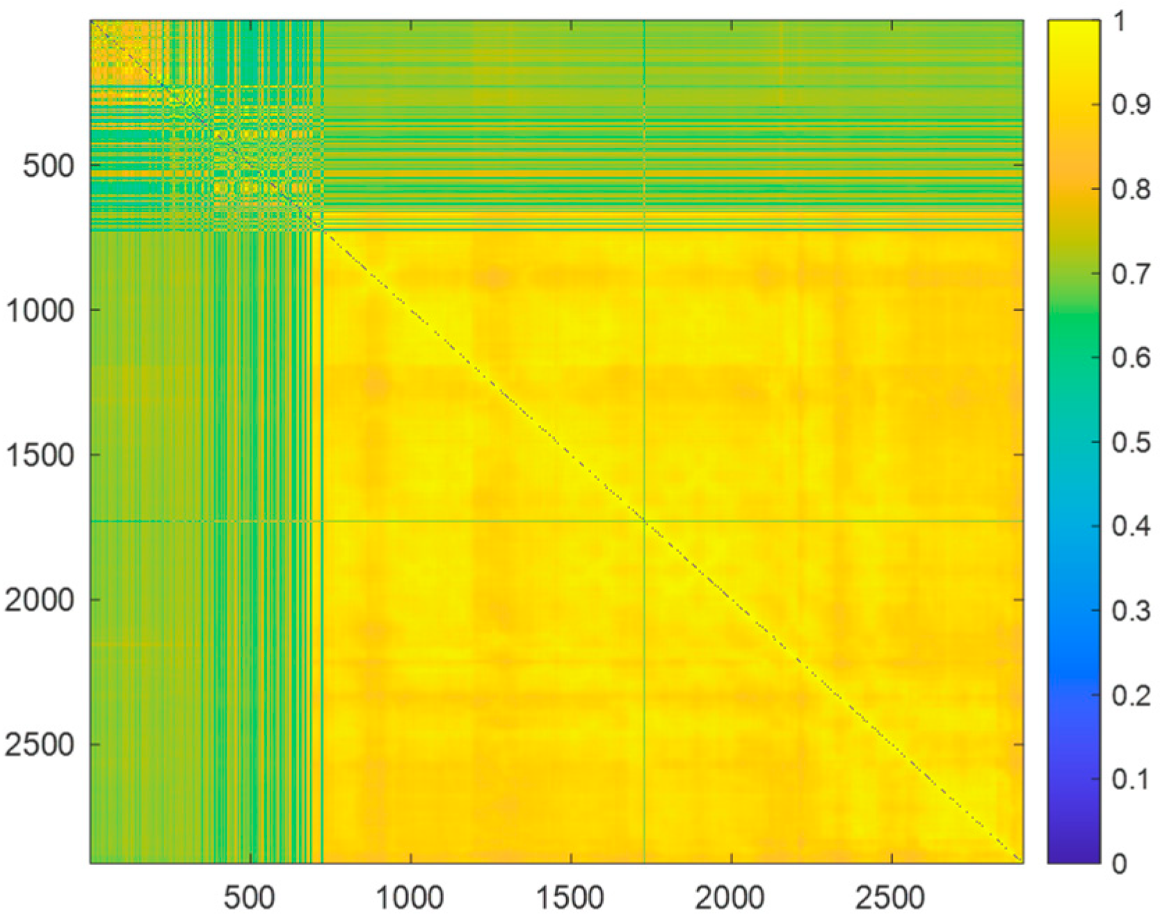
4.2. Construction of the Similarity Matrix

The structural similarity index measures (SSIM) [41] are used in this paper to extract time-frequency image features and measure the similarity between different pulse time-frequency images. Compared with feature extraction algorithms, such as SIFT and Kaze, SSIM can effectively distinguish time-frequency images with the same modulation type but different modulation parameters, and it can also deal with unknown modulation types effectively. SSIM compares the similarity between different images in terms of brightness, contrast, and structure, and it can compare the overall image and local similarity. For image x and image y, the SSIM is calculated as follows:

$$SSIM(x,y)={[l(x,y)]}^{\alpha }\cdot {[c(x,y)]}^{\beta }\cdot {[s(x,y)]}^{\gamma }$$

(7)

where $l(x,y)$, $c(x,y)$, and $s(x,y)$ represent the luminance term, the contrast term, and the structure terms, respectively. $\alpha$, $\beta$, and $\gamma$ are their weights. The terms are calculated as follows:

$$l(x,y)=\frac{2{\mu }_x{\mu }_y+C_1}{{\mu }_x{}^2+{\mu }_y{}^2+C_1}$$

(8)

$$c(x,y)=\frac{2{\sigma }_x{\sigma }_y+C_2}{{\sigma }_x{}^2+{\sigma }_y{}^2+C_2}$$

(9)

$$s(x,y)=\frac{{\sigma }_{xy}+C_3}{{\sigma }_x{\sigma }_y+C_3}$$

(10)

where ${\mu }_x$ and ${\mu }_y$ are the local means for the images, ${\sigma }_x$ and ${\sigma }_y$ are the standard deviations for the images, and ${\sigma }_{xy}$ is the cross-covariance for the images. $C_1$, $C_2$, $C_3$ are the non-zero regularization constants to avoid instability for image regions where the local mean or standard deviation is close to zero. If $\alpha =\beta =\gamma =1$, and $C_3=C_2/2$, at this point, the SSIM can be simplified to the following:

$$SSIM(x,y)=\frac{(2{\mu }_x{\mu }_y+C_1)(2{\sigma }_{xy}+C_2)}{({\mu }_x{}^2+{\mu }_y{}^2+C_1)({\sigma }_x{}^2+{\sigma }_y{}^2+C_2)}$$

(11)

The SSIM is usually obtained between 0 and 1, and the closer it is to 1, the smaller the deference between images. Figure 2 displays the local SSIM map and the global SSIM value after the 2-D Wiener filtering noise reduction for the TFIs belonging to the same emitter as well as different emitters in a section of the received signal. The rightmost column of images are the results of SSIM (local SSIM maps), and the values (“SSIM Val”) are the global SSIM values.

Among them, pulse 1537 and pulse 1539, pulse 1541 and pulse 1560 come from two different radiation sources, respectively. It can be seen that SSIM has good differentiation between signal pulses belonging to different radiation sources in similar background noise environments, which can provide support for the next step of pulse TFI clustering.

In the actual signal reception process, it can be considered that the signal-to-noise ratio (SNR) remains unchanged during the acquisition of the same segment of signal data, so the feature extraction and matching in the dynamic SNR environment are not considered in this paper for the time being.

After obtaining the SSIM values between individual pulses, the SSIM similarity matrix S, where S(x, y) is the SSIM value between pulse x and pulse y, is constructed.

4.3. Affinity Propagation Clustering of the Similarity Matrix

AP clustering is performed on the similarity matrix to obtain the TFI pseudo-labeled dataset. The basic method of AP clustering is to treat all samples as nodes of the network and to iteratively update the responsibility and availability among the nodes in the network [42], where Responsibility (R) is used to describe the degree of suitability of sample y as the cluster center of the category in which sample x is located (Equation (12)). The Availability (A) is used to describe the degree of suitability of sample x in selecting sample y as its cluster center (Equation (13)), and z represents the samples other than x and y within the dataset.

$$R(x,y)=S(x,y)-\max [R(x,z)+S(x,z)],z\ne y$$

(12)

$$A(x,y)=\left\{\begin{array}{ll}\min \{R(y,y)+{\displaystyle \sum _{z\ne x,z\ne y}\max [0,R(z,y)],0\}}\hfill & , x\ne y\hfill \\ {\displaystyle \sum _{z\ne y}\max [0,R(z,y)]}\hfill & , x=y\hfill \end{array}\right.$$

(13)

As can be seen, the responsibility and availability degrees are calculated by including not only the current samples x and y but also other samples z in addition to them. Multiple iterations are performed until several high-quality clustering centers are selected to maximize the sum of similarity between each clustering center and the samples, and the remaining nodes are assigned to each clustering center.

The AP clustering is based on the similarity matrix of the samples, with the diagonal elements of the matrix being all zeros, which means that each sample can be a cluster center. Initialize the responsibility matrix R and the availability matrix A as all-0 matrices and set the damping factor $\lambda$. And then, matrix R and matrix A are updated using Equation (14), which can be expressed as follows after n iterations:

$$\left\{\begin{array}{l}{R}_n(x,y)=\lambda R_{n-1}(x,y)+(1-\lambda )\{S(x,y)-\max [A_n(x,z)+S(x,z)]\},z\ne y\hfill \\ A_n(x,y)=\lambda A_{n-1}(x,y)+(1-\lambda )\min \{0,R_n(y,y)+{\displaystyle \sum _{z\ne x,z\ne y}\max [0,R_n(z,y)]\}}\hfill \\ A_n(y,y)=\lambda A_{n-1}(x,y)+(1-\lambda ){\displaystyle \sum _{z\ne y}\max [0,R_n(z,y)]}\hfill \end{array}\right.$$

(14)

The iteration is terminated until the clustering results no longer change after several iterations or other convergence conditions are met. At this point, we get the decision matrix E = R + A; the xth row of the matrix E corresponds to the sample x; find the number of columns y where the maximum value in the row is located, as in Equation (15), to get the cluster exemplars corresponding to each sample:

$$c_x=\arg {\max }_y[A(x,y)+R(x,y)],\forall x$$

(15)

If the element E(x, x) on the diagonal of the matrix E satisfies E(x, x) > 0, then the sample x itself is a cluster center. The damping factor $\lambda$ satisfies $\lambda \in [0,1)$, which is used to control the convergence speed of the iterations. If the damping factor is too large, the number of iterations required for convergence is high, which slows down the computational speed. Conversely, if the damping factor is too small, R and A will have a large oscillation in the iterative process, and it is difficult to converge. The damping factor is typically set to a value between 0.9 and 0.99 based on engineering experience. The overall flowchart of the AP clustering algorithm is shown in Figure 3.

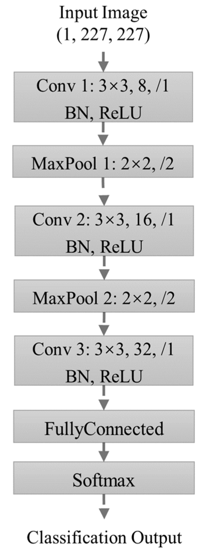
4.4. Network Structure of the Constructed CNN

Although the unsupervised clustering algorithm can divide the TFI dataset into multiple classes, it is computationally intensive. Therefore, this paper uses the AP clustering algorithm to initially probe the number of radiation sources that may be contained in the signal and constructs a pseudo-labeled dataset to train a neural network to classify the remaining TFIs. To improve the training efficiency while ensuring the recognition rate, this paper constructs a lightweight CNN, as shown in Figure 4.

The network input is a grayscale image of size 227 × 227 × 1. The three convolutional layers Conv 1, Conv 2, and Conv 3 contain 8, 16, and 32 convolutional kernels, respectively, all with a convolutional kernel size of 3 × 3 and a step size of 1. Two maximum pooling layers with a pooling kernel size of 2 × 2 and a pooling step size of 2 are placed between Conv 1 and Conv 2 and Conv 2 and Conv 3, respectively. The output layer is activated using the Softmax function, and all other layers are activated using the ReLU function.

The training of a convolutional neural network involves error minimization by calculating the error between the network output and the target to continuously adjust the weights between neurons in the network. After the initialization of the network, it can be roughly divided into two stages, forward propagation and error back propagation. In the forward propagation stage, the input training data is propagated forward through the convolutional, pooling, and fully connected layers to obtain the output value, and the bias between the output value and the target is found. If the bias is lower than the expected value, the training is finished. If the bias is higher than the expected value, the error backpropagation stage is entered, and the bias is passed back to the network. The errors of the fully connected, pooling, and convolutional layers are found in turn. The weights of each layer are updated according to the gradient of the error to optimize the network, and then enter a new iteration of training.

The key in the training process is to set an objective function that measures the bias between the output value and the target value and a reasonable network optimization algorithm. In this paper, the convolutional neural network is used to classify the pulse time-frequency images, so the cross entropy, which measures the difference between the true probability distribution and the estimated probability distribution, is used as the objective function. For the input x, suppose there are N samples, the true probability distribution of x is p, and the probability distribution calculated by the network is q. Then the cross entropy (H) of p and q is as follows:

$$H(p,q)=-{\displaystyle \sum _{i=1}^{N}p(x_i)\log q(x_i)}$$

(16)

Assume the network model to be $g(x,\theta )$, where $\theta$ represents each parameter in the network model, the network optimization algorithm minimizes the objective function by taking the gradient of the objective function with respect to each parameter in $\theta$ and then updating each element in the direction of decreasing gradient, i.e., the idea of gradient descent. Suppose the training sample pair is $\{x_n,y_n\},n=1,\dots ,N$, the search step length (also called learning rate) is $\lambda$, and the optimized objective function is $L(\cdot )$; then the parameters ${\theta }_{t+1}$ in the (t + 1)th training iteration are as follows:

$$\begin{array}{cc}\hfill {\theta }_{t+1}& ={\theta }_t-\lambda \frac{1}{N}{\displaystyle \sum _{n=1}^N\frac{\partial L(y_n,g(x_n,{\theta }_t))}{\partial {\theta }_t}}\hfill \\ & ={\theta }_t-\lambda \nabla L(\theta )\hfill \end{array}$$

(17)

where $\nabla (\cdot )$ stands for finding the gradient. Common gradient descent-based optimization algorithms include Stochastic Gradient Descent (SGD), Stochastic Gradient Descent Momentum (SGDM), Batch Gradient Descent), etc. In this paper, the SGDM method is used as the network optimization algorithm. The SGDM method smooths the current gradient based on the exponentially weighted average of the historical gradients (i.e., “momentum”), which reduces the oscillation when updating the weights to accelerate the convergence. The (t + 1)th round of training of the SGDM method has the following parameters:

$${\theta }_{t+1}={\theta }_t-\lambda m_t$$

(18)

where the iterative update of the momentum $m_t$ is as follows:

$$m_t={\beta }_1\cdot m_{t-1}+(1-{\beta }_1)\cdot \nabla L(\theta )$$

(19)

${\beta }_1$ is a predefined hyperparameter.

4.5. Data Augmentation

In this paper, data augmentation techniques, including random resized crop and Gaussian noise, are used to expand the dataset. These techniques enhance the diversity of the samples and improve the model’s ability to generalize. In detail, “random resized crop” randomly crops the region on the original TFI and then resizes it to a given size, thereby improving the model’s generalization ability. “Gaussian noise” adds zero-average Gaussian noise to the original image, which distorts high-frequency features and enhances the learning ability of the CNN.

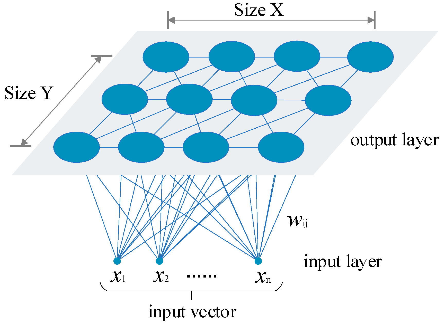
4.6. Refined Sorting Using the SOM Network

After the self-supervised clustering based on the pulse time-frequency image features, the original pulse stream with severe overlap is sorted into several pulse groups with the same intra-pulse modulation type and similar intra-pulse modulation parameters. The SOM network is then trained with the pulse width, carrier frequency, and bandwidth of individual pulses as training inputs for the pulse groups of interest. The pulses within the groups are further sorted.

The SOM network structure contains two parts: the input layer and the output layer (also called the mapping layer or the competition layer), and its structure is shown in Figure 5.

In this figure, the training sample of the SOM network is an n-dimensional vector $X=(x_1,x_2,\dots ,x_n)$. The neurons in the input layer are arranged in a single layer with the same dimensions as the input sample. The competition layer is generally a two-dimensional planar structure, and each output of the competition layer neurons corresponds to one input pattern. The number of neurons determines the granularity and size of the model, which affects the accuracy and generalization ability of the network. The input layer is fully connected to the competition layer, and the neurons in the competition layer are laterally inhibited. There are m neurons in the competitive layer in the figure, where the connection weight between the jth neuron and the input layer is $W_j=(w_{1,j},w_{2,j},\dots ,w_{n,j})$; $w_{i,j}$ represents each component of the connection weight, $i=1,2,\dots ,n$, $j=1,2,\dots ,m$.

The implementation of unsupervised clustering using the SOM network includes two main steps: training and clustering. Training can be further divided into three phases: initialization, competition, and iteration. In the initialization phase, the input data are normalized, the network structure is defined, each weight component $w_{i,j}(0)\in [0,1]$ is randomly initialized, a larger initial value of the winning neighborhood radius ${\phi }_{j*}(0)$ is set, and parameters, such as the learning rate $\alpha (t)$, and the maximum number of training sessions is defined. In the competition phase, the Euclidean distance d_j between the input sample vector and the neurons in the competition layer is calculated using the following equations, and the closest neuron is used as the winning neuron $j*$.

$$\begin{array}{cc}\hfill d_j& =‖X-W_j‖\hfill \\ & =\sqrt{{\displaystyle \sum _{i=1}^n{(x_i-w_{i,j})}^2}},j=1,2,\dots ,m\hfill \end{array}$$

(20)

$$d_{j*}=\min (d_j)$$

(21)

Several neurons in the neighborhood of the winning neuron are taken as the winning region. In the iteration phase, the weights of each neuron in the winning region are updated iteratively:

$$w_{i,j}(t+1)=w_{i,j}(t)+\alpha (t)\cdot [x_i-w_{i,j}(t)],i=1,2,\dots ,n$$

(22)

Moreover, the radius of the winning neighborhood decreases dynamically as the number of iterations (N_train) increases and remains constant after reaching 1.

$${\phi }_{j^{*}}(t)=⌈{\phi }_{j*}(0)\cdot (1-\frac{t}{N_{train}})⌉,{\phi }_{j*}(t)\ge 1$$

(23)

After multiple iterations, the winning region is reduced round by round until the winning region contains only one winning neuron or reaches the maximum number of iterations. Eventually, the minimized winning region is labeled as a response to a specific class of inputs.

In the clustering step, input samples cause the neurons in the corresponding regions of the competing layers to be excited, and new winning neurons are obtained. From the perspective of neurons, each neuron represents a category, and the number of samples in each category can be represented by the hit map of the corresponding neuron. From the perspective of samples, samples with the same or similar neighbors of the winning neuron can be grouped into the same category, and new samples that did not appear in the previous training are assigned to the most similar neurons.

The processing flow of this section is as follows:

• Select clusters of subject pulses;
• Randomly select 50% of the pulses as the training set and the rest as the test set, and construct the SOM network;
• Train the SOM network with the pulse width, carrier frequency, and bandwidth of each pulse in the cluster as input;
• Clustering the pulse clusters using the SOM network;
• Merge the similar clustering centers, store the clustering centers with fewer numbers within the category and distant from other centers, set them as new pulse clusters, and repeat steps 3~5.

After clustering using the SOM, if there is still a small number of pulses failing to be clustered reasonably, they will need to be analyzed further. The analysis determines if they belong to any existing clusters or new pulse groups or if they are interfering with pulses.

5. Simulations and Analyses

This section first tests the performance of the AP-CNN based self-supervised clustering method. And then, the proposed method is compared with traditional methods based on SVM and KNN, as well as machine learning methods of the ResNet 50 network and CL-CNN. All methods are configured with the best performance, obtained by 50 trials. The simulation platform is MATLAB(R) R2021a software, the processor is Intel(R) Core(TM) i7-10850H CPU @ 2.70 GHz, and the GPU is Nvidia(R) GeForce(TM) RTX 2060. During the experiments, we used the Parallel for-loop of MATLAB software in order to distribute the computation process of the similarity matrix to each core of the CPU, which may improve the hardware utilization and accelerate the computation speed.

5.1. Dataset Description

The experimental setup contains a signal environment of five radars, each with different parameter settings, as listed in

Table 1. Parameter settings of radars.

Radars	Intra-Pulse Modulation Type	Carrier Frequency (MHz)	Bandwidth (MHz)	Pulse Width (μs)	PRI (μs)
A	constant frequency	7500	-	1000	1.73
B	LFM	1275	80	33	2.64
C	LFM	4600	20	20	2.52
D	VFM	2400	50	65	3.1
E	OFDM-LFM	5300	45	40	1.62

, where OFDM-LFM has eight code words, i.e., eight sub-pulses of equal time width.

For each radar, 3000 simulated signal samples are generated, and Gaussian white noise is added to vary the signal-to-noise ratio from −10 dB to 30 dB. After down-conversion, SPWVD is applied to each signal sample to obtain the TFI dataset to be sorted. There is partial overlap between the radar parameters set by the simulation, and, as shown in Figure 6, the time-frequency images have different degrees of overlap to reflect the performance of the clustering method proposed in this paper.

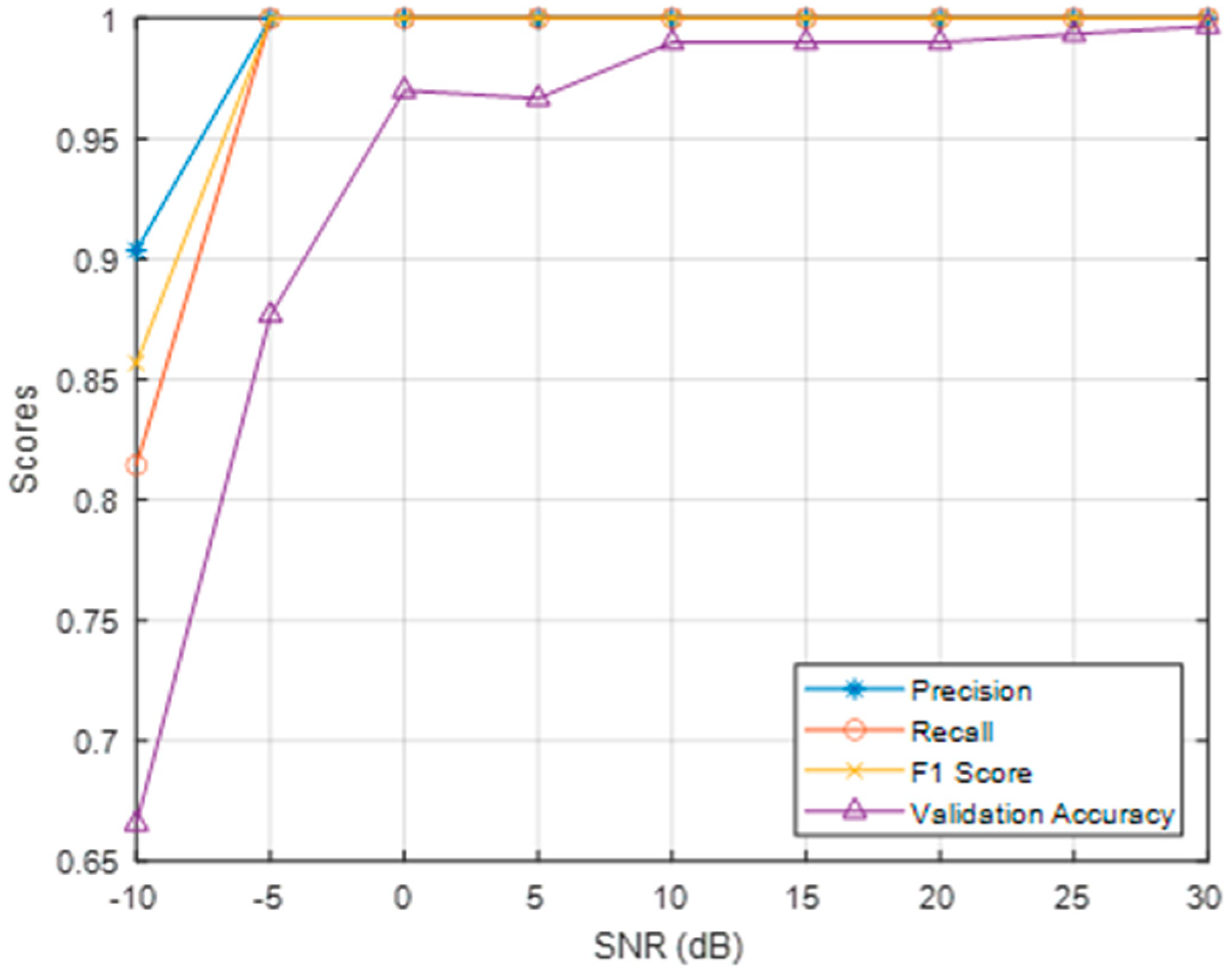
5.2. Performance Testing of the Proposed Sorting Method

In signal environments with different signal-to-noise ratios, 20% of the pulse time-frequency images are randomly selected from the dataset and sorted using AP clustering on their obtained similarity matrices. The damping factor $\lambda$ is set to 0.995, and the maximum number of iterations is 10,000. The clustering results are evaluated using precision, recall, and F1 score, calculated as follows:

$$\mathrm{Precision}=\frac{\mathrm{TP}}{\mathrm{TP}+\mathrm{FP}}$$

(24)

$$\mathrm{Recall}=\frac{\mathrm{TP}}{\mathrm{TP}+\mathrm{FN}}$$

(25)

$$\mathrm{F}1\mathrm{score}=\frac{2\times \mathrm{Precision}\times \mathrm{Recall}}{\mathrm{Precision}+\mathrm{Recall}}$$

(26)

where TP, TN, FP, and FN represent the number of true positives, true negatives, false positives, and false negatives, respectively. The results are shown in Figure 7.

All five radars were found by AP clustering in the experiment. Based on this, the method accurately clustered the pulse time-frequency images, achieving an accuracy, recall, and F1 score of no less than 0.987 when the SNR is higher than −5 dB. However, the performance of clustering decreases after the signal-to-noise ratio falls below −5 dB.

At each SNR from −10 dB to 30 dB, from the AP clustering results generated from the previous experiments, 80% are randomly extracted as the training set, 10% as the validation set, and 10% as the test set. To optimize the dataset obtained from AP clustering, the results in which the classification is obviously wrong are excluded, and the training set samples are augmented to improve the generalization performance. The lightweight CNN constructed in Section 4.4 is trained with the main training parameters set, as shown in

Table 2. Main training parameter settings for training.

Parameter Name	Parameter Value
Solver	SGDM
Mini Batch Size	100
Max Epochs	20
Initial Learning Rate	0.001
Learning Rate Decay Period	10
Learning Rate Decay Factor	0.1
Shuffle	Every epoch

.

The trained CNN classifies the remaining 80% of the pulse time-frequency images. The precision, recall, F1 score, and validation accuracy of the classification results at different SNRs are shown in Figure 8.

The experiment demonstrates that the AP-CNN self-supervised clustering algorithm proposed in this paper has good performance. The lightweight CNN, trained with the pseudo-labeled dataset automatically constructed by AP clustering, can classify the massive pulse data quickly and accurately. The accuracy, recall, and F1 score at 0 dB are no less than 0.9993, and the accuracy of the validation set is no less than 0.97. However, the results of AP clustering are partially confounded after the SNR is below −5 dB, and the effect of training CNN starts to decrease, which consequently reduces the performance of CNN. Figure 9 shows examples of pulse time-frequency images of five radars at −10 dB, and Figure 10 shows the confusion matrix of the self-supervised clustering results.

Notably, in the low SNR environment, the time-frequency images are seriously affected by noise, and the unsupervised AP clustering may not be able to effectively distinguish all the radars. However, it can still achieve more accurate sorting for the significantly differentiated Radar A, Radar B, and Radar D. In the actual signal sorting process, we can extract the time-frequency images of the emitters with better sorting results and then carry out further sorting of the remaining pulses combined with intra- and inter-pulse parameters, which can significantly reduce the need for manual operation and improve the efficiency of signal sorting.

For Radar C and Radar E, their 6000 TFIs are still mixed after self-supervised clustering. The SOM network is built using the selforgmap function of MATLAB software to differentiate the individual pulses based on their carrier frequency, bandwidth, and pulse width. The competition layer of the SOM network contains 12 neurons, the initial value of the winning neighborhood radius is 3, and the maximum number of iterations is 30. Different SNRs from −10 dB to 30 dB are set to test the clustering accuracy of the SOM algorithm. The accuracy is calculated as follows:

$$\mathrm{Accuracy}=\frac{\mathrm{TP}+\mathrm{TN}}{\mathrm{TP}+\mathrm{TN}+\mathrm{FP}+\mathrm{FN}}$$

(27)

Figure 11 shows the accuracy at each SNR.

It can be seen that the accuracy is consistently high across all SNRs tested, with a minimum accuracy of 0.96 at 0 dB SNR. The experiments also demonstrate that the unsupervised AP clustering part of the proposed self-supervised clustering method can effectively discover the unknown radiation sources and perform feature extraction and preliminary classification; the results of the unsupervised clustering are optimized, and the dataset is constructed, and a lightweight CNN is trained accordingly, which can quickly and accurately classify massive pulses and improve the efficiency of signal analysis.

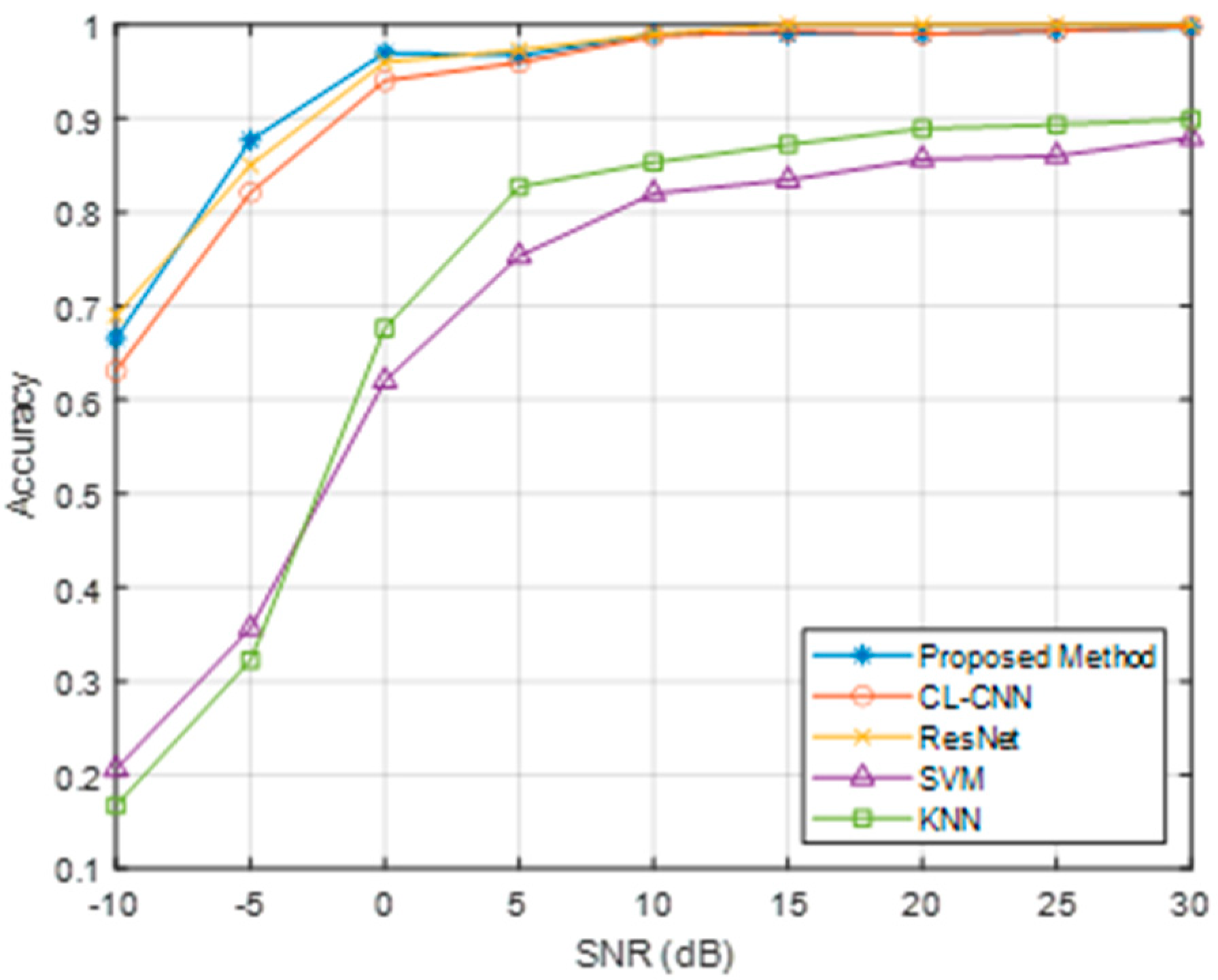
5.3. Performance Comparison

Comparisons are made with traditional methods based on KNN, SVM, and machine learning methods based on ResNet 50 network and CL-CNN. All methods are configured with the best performance, obtained through 50 experiments.

Firstly, the anti-noise performance is compared. The results of sorting using five methods at different signal-to-noise ratios are shown in Figure 12, and it can be seen that the accuracy of the proposed method in this paper is improved compared to SVM and KNN methods. Compared with other machine learning-based methods, the accuracy at each SNR is no lower than that of CL-CNN and close to that of ResNet 50. The confusion between radar C and radar E is more serious after the SNR is below −5 dB, which reduces classification accuracy.

And then, the classification accuracy of each radar by different methods is compared at the same SNR. The SNR is set to −5 dB. The results are shown in

Table 3. Comparison of the classification accuracy of five radars by different methods (−5 dB).

Methods	Radar A	Radar B	Radar C	Radar D	Radar E
Proposed Method	0.8690	0.8923	0.8347	0.9037	0.8437
CL-CNN	0.8237	0.8813	0.7323	0.8567	0.7667
ResNet	0.8317	0.8917	0.8377	0.8793	0.8217
SVM	0.3413	0.3633	0.3323	0.4713	0.2617
KNN	0.3533	0.3123	0.3217	0.4327	0.2413

.

It can be seen that the proposed method has a good classification accuracy for each radar. For differentiating Radar A, Radar B, and Radar D, which are more distinguishable, the effect achieved by the proposed method is close to that of the CL-CNN and ResNet 50-based methods. For differentiating Radar C and Radar E, which are easily confused, the effect achieved by the proposed method’s differentiation ability is close to that of the ResNet 50 method and higher than that of the CL-CNN method. It is also noted that the performance of all three machine learning-based methods is significantly higher than that of the traditional SVM and KNN methods due to their stronger feature extraction capability. Overall, these results suggest that the proposed method is a promising approach for radar signal sorting.

6. Validation Based on Measured Data

In this section, we apply the proposed method to process the measured data that contains a certain type of SAR, a test radar, as well as other unknown emitter signals. We compare it with the sorting methods based on SVM, KNN, ResNet 50 network, and CL-CNN mentioned in the previous section, and all methods are configured with the best performance. It should be noted that the number of radiation sources and parameters included in the measured data is unknown before sorting.

6.1. Dataset Description

The dataset contains a total of 7500 pulses from a SAR (Radar F) and a test conventional radar (Radar G), as well as signals from other unknown radiation sources.

Table 4. Parameter settings of Radar F and Radar G.

Radars	Intra-Pulse Modulation Type	Carrier Frequency (MHz)	Bandwidth (MHz)	Pulse Width (μs)	PRI (μs)
F	LFM	8620	150	111	1.852
G	LFM	8650	110	45	1.793

shows the parameter settings of Radar F and Radar G. The receiver automatically analyzes the arrival angle, arrival time, carrier frequency, pulse width, bandwidth, and pulse amplitude of the signal, and the signal-to-noise ratio is about 5 dB.

After down-conversion of the received signal, SPWVD is performed to obtain the TFI dataset for sorting.

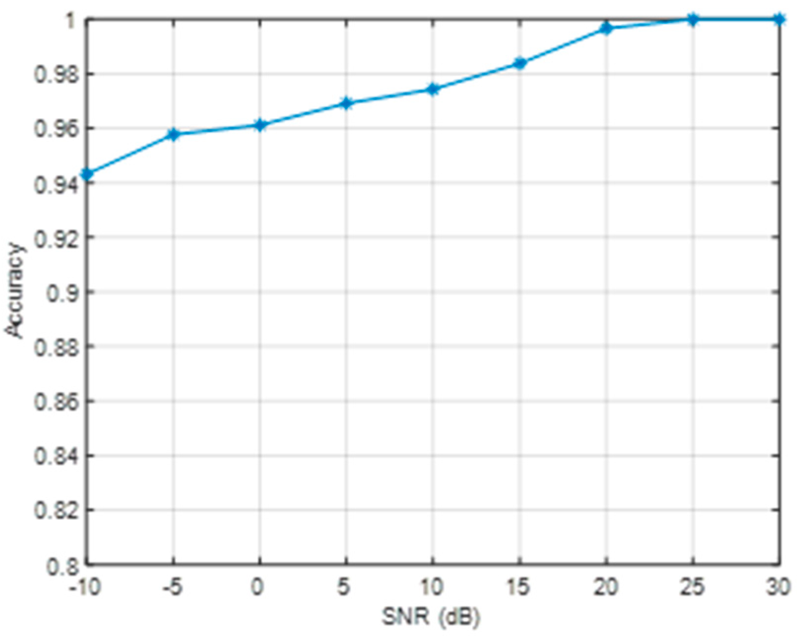
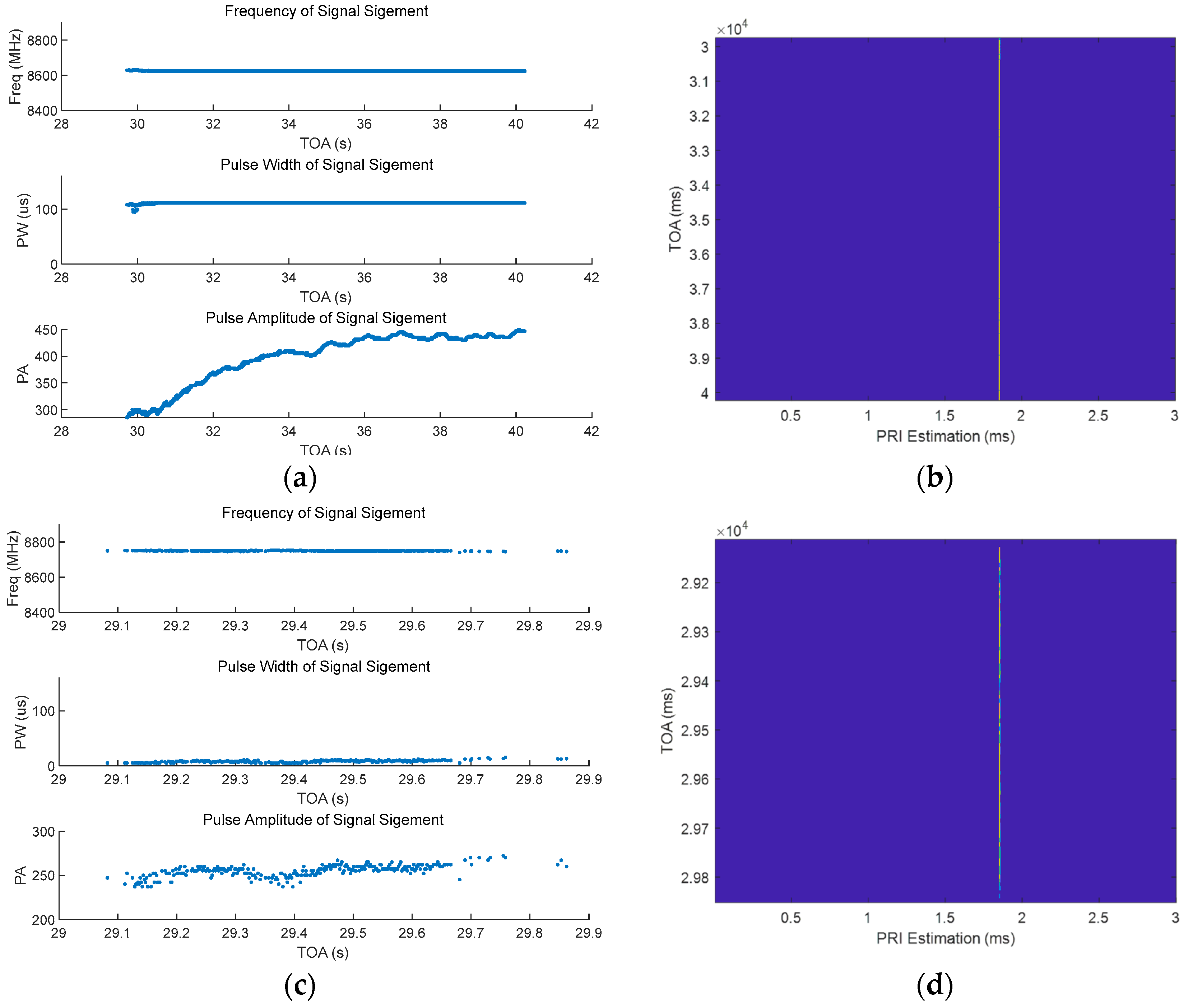
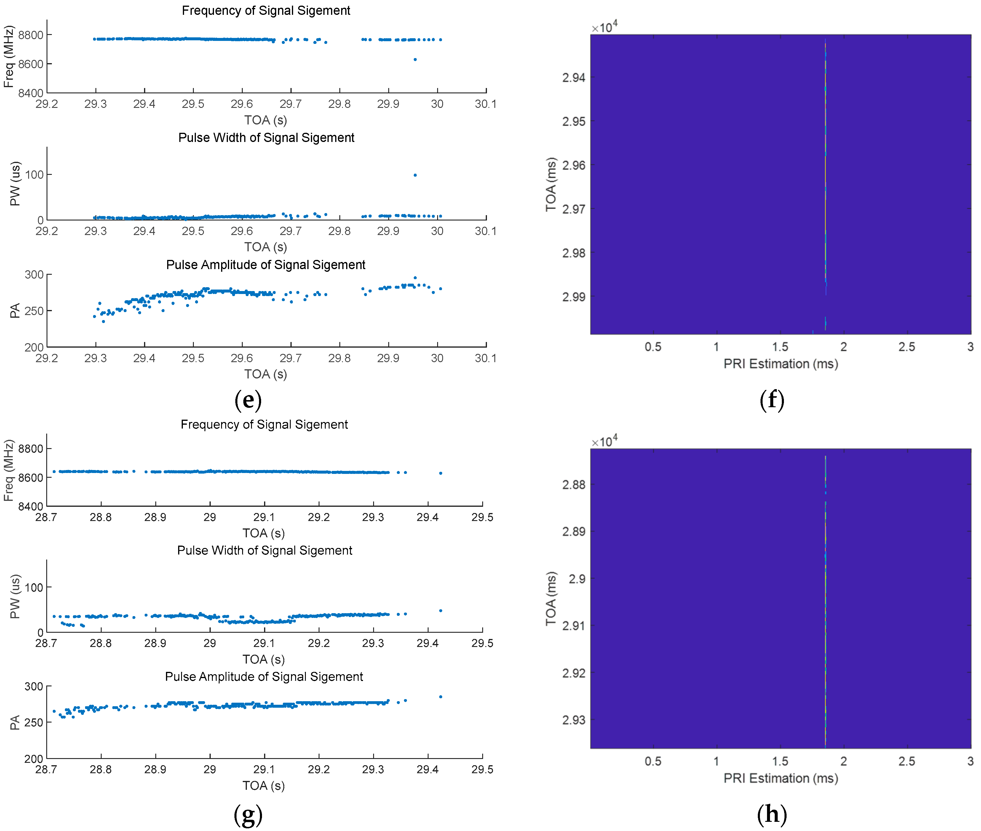
6.2. Performance Testing of the Proposed Sorting Method Using Measured Data

The TFI dataset is processed using the proposed method, and 40% of the images are randomly selected to obtain their similarity matrix. The similarity matrix is shown in Figure 13.

The existence of obvious rectangular partitions in the similarity matrix indicates the existence of pulses that are well differentiated in the time-frequency domain. Using AP-CNN, 13 classes are obtained, and the confusion matrix of the validation dataset is shown in Figure 14.

The four classes containing the largest number of pulses, Class_739, Class_348, Class_454, and Class_169, were selected for analysis, and their carrier frequencies, pulse widths, amplitudes, and PRIs are shown in Figure 15.

The AP-CNN method sorts the dataset into several classes with high intra-class similarity. Matching the sorting results with the parameters of the radars used in the experiment, it is observed that the parameters of Class_739 match those of Radar F, and the parameters of Class_169 match those of Radar G.

However, the parameters of Class_348 and Class_454 have a certain degree of overlap and may come from the same radiation source. Therefore, they are mixed and further sorted using a SOM network based on their carrier frequency, bandwidth, and pulse width. The competition layer of the SOM network contains 9 neurons, the initial value of the winning neighborhood radius is 3, and the maximum number of iterations is 30. Figure 16 shows the hit map of each neuron after sortin; the number in the neurons represents the sample number of the neuron.

It can be seen that Class_348 and Class_454 are attributed to two adjacent neurons, indicating that they may belong to different radiation sources or different working modes of the same emitter.

6.3. Performance Comparison

Comparisons are made with methods mentioned in the previous section—traditional methods based on KNN, SVM, and machine learning methods based on ResNet 50 network and CL-CNN. All methods are configured with the best performance, obtained through 50 experiments. The classification performance of each radar is compared. The results are shown in

Table 5. Comparison of the classification accuracy of two radars by different methods (−5 dB).

Methods	Radar F	Radar G
Proposed Method	0.8620	0.8733
CL-CNN	0.8012	0.8567
ResNet	0.8318	0.8913
SVM	0.3117	0.3260
KNN	0.3018	0.3113

.

The proposed method achieves better classification performance for both radars than all other methods, with significantly higher accuracy than SVM and KNN, as well as the CL-CNN and ResNet-based methods. The proposed method is better able to distinguish signals with the same intra-vehicle modulation type and similar parameters compared to CL-CNN. Compared with ResNet, the proposed method does not require a large amount of manual operations to construct the training dataset.

However, in the process of actual sorting, the proposed method may differentiate signals belonging to the same emitter into multiple ones. Further examination and professional interpretation are needed to determine whether the sorting results of AP-CNN and SOM networks need to be optimized. Meanwhile, the training dataset of AP-CNN can be further improved by “human-in-the-loop” refinement, which will benefit the performance of the proposed method. In this experiment, we also noticed that calculating the similarity matrix and performing affinity propagation clustering require a significant amount of memory. Future research can further explore how to reduce the dependence on manual operation, make the method more efficient and intelligent, and then improve the applicability and reliability of the method in the field.

7. Conclusions

In this paper, we propose a self-supervised clustering-based method for sorting SAR radiation sources, which achieves the clustering and sorting of an unknown number of noncooperative target pulse-time frequency images by self-supervised clustering of the SSIM features, and optimizes the sorting results by using SOM networks. We evaluated the proposed method using both simulated and measured data and compared it with conventional methods based on KNN and SVM, as well as machine learning methods based on ResNet and CL-CNN. Simulation experiments demonstrate that the proposed method outperforms the other four methods in terms of classification accuracy and also exhibits robustness against noise. The experiments using measured data tested the effectiveness of our proposed method. Particularly, the proposed method can effectively alleviate the shortage of labeled signal data and reduce the need for manual operation. Therefore, our future research will focus on improving the efficiency and intelligence of the method to improve its applicability and reliability.

References

1. Gupta, M.; Hareesh, G.; Mahla, A.K. Electronic warfare: Issues and challenges for emitter classification. Def. Sci. J. 2011, 61, 228. [Google Scholar] [CrossRef] [Green Version]
2. Qu, Z.; Mao, X.; Deng, Z. Radar signal intra-pulse modulation recognition based on convolutional neural network. IEEE Access 2018, 6, 43874–43884. [Google Scholar] [CrossRef]
3. Yuan, S.; Li, P.; Wu, B.; Li, X.; Wang, J. Semi-supervised classification for intra-pulse modulation of radar emitter signals using convolutional neural network. Remote Sens. 2022, 14, 2059. [Google Scholar] [CrossRef]
4. Villano, M.; Krieger, G.; Moreira, A. Nadir echo removal in synthetic aperture radar via waveform diversity and dual-focus postprocessing. IEEE Geosci. Remote Sens. Lett. 2018, 15, 719–723. [Google Scholar] [CrossRef]
5. Villano, M.; Krieger, G.; Moreira, A. Waveform-Encoded SAR: A Novel Concept for Nadir Echo and Range Ambiguity Suppression. In Proceedings of the EUSAR 2018, 12th European Conference on Synthetic Aperture Radar, Aachen, Germany, 4–7 June 2018. [Google Scholar]
6. Mittermayer, J.; Martinez, J.M. Analysis of Range Ambiguity Suppression in SAR by up and down Chirp Modulation for Point and Distributed Targets. In Proceedings of the IGARSS 2003, 2003 IEEE International Geoscience and Remote Sensing Symposium, Proceedings (IEEE Cat, No.03CH37477), Toulouse, France, 21–25 July 2003; Volume 6, pp. 4077–4079. [Google Scholar]
7. Jeon, S.-Y.; Kraus, T.; Steinbrecher, U.; Villano, M.; Krieger, G. A TerraSAR-X Experiment for Validation of Nadir Echo Suppression through Waveform Encoding and Dual-Focus Postprocessing. In Proceedings of the European Conference on Synthetic Aperture Radar (EUSAR) 2021, Leipzig, Germany, 29 March–1 April 2021. [Google Scholar]
8. Wang, R.; Chen, J.; Wang, X.; Sun, B. High-Performance Anti-Retransmission Deception Jamming Utilizing Range Direction Multiple Input and Multiple Output (MIMO) Synthetic Aperture Radar (SAR). Sensors 2017, 17, 123. [Google Scholar] [CrossRef] [PubMed] [Green Version]
9. Song, C.; Wang, Y.; Jin, G.; Wang, Y.; Dong, Q.; Wang, B.; Zhou, L.; Lu, P.; Wu, Y. A Novel Jamming Method against SAR Using Nonlinear Frequency Modulation Waveform with Very High Sidelobes. Remote Sens. 2022, 14, 5370. [Google Scholar] [CrossRef]
10. Kersten, P.; Lee, J.-S.; Ainsworth, T. Unsupervised Classification of Polarimetric Synthetic Aperture Radar Images Using Fuzzy Clustering and EM Clustering. IEEE Trans. Geosci. Remote Sens. 2005, 43, 519–527. [Google Scholar] [CrossRef]
11. Zhang, C.; Liu, Y.; Si, W. Synthetic Algorithm for Deinterleaving Radar Signals in a Complex Environment. IET Radar Sonar Navig. 2020, 14, 1918–1928. [Google Scholar] [CrossRef]
12. Cheng, W.; Zhang, Q.; Dong, J.; Wang, C.; Liu, X.; Fang, G. An Enhanced Algorithm for Deinterleaving Mixed Radar Signals. IEEE Trans. Aerosp. Electron. Syst. 2021, 57, 3927–3940. [Google Scholar] [CrossRef]
13. Su, S.; Fu, X.; Zhao, C.; Yang, J.; Xie, M.; Gao, Z. Unsupervised K-Means Combined with SOFM Structure Adaptive Radar Signal Sorting Algorithm. In Proceedings of the 2019 IEEE International Conference on Signal, Information and Data Processing (ICSIDP), Chongqing, China, 11–13 December 2019. [Google Scholar] [CrossRef]
14. Chen, X.; Liu, D.; Wang, X.; Chen, Y.; Cheng, S. Improved DBSCAN Radar Signal Sorting Algorithm Based on Rough Set. In Proceedings of the 2021 2nd International Conference on Big Data and Informatization Education (ICBDIE), Hangzhou, China, 2–4 April 2021. [Google Scholar] [CrossRef]
15. Zhao, Z.; Zhang, H.; Gan, L. A Multi-Station Signal Sorting Method Based on TDOA Grid Clustering. In Proceedings of the 2021 IEEE 6th International Conference on Signal and Image Processing (ICSIP), Nanjing, China, 22–24 October 2021. [Google Scholar] [CrossRef]
16. Mottier, M.; Chardon, G.; Pascal, F. Deinterleaving and Clustering Unknown RADAR Pulses. In Proceedings of the 2021 IEEE Radar Conference (RadarConf21), Atlanta, GA, USA, 7–14 May 2021; pp. 1–6. [Google Scholar] [CrossRef]
17. Wang, G.; Chen, S.; Hu, X.; Yuan, J. Radar Emitter Sorting and Recognition Based on Time-Frequency Image Union Feature. In Proceedings of the 2019 IEEE 4th International Conference on Signal and Image Processing (ICSIP), Wuxi, China, 19–21 July 2019. [Google Scholar] [CrossRef]
18. Kong, S.-H.; Kim, M.; Hoang, L.M.; Kim, E. Automatic LPI radar waveform recognition using CNN. IEEE Access 2018, 6, 4207–4219. [Google Scholar] [CrossRef]
19. Tang, Q.; Huang, H.-H.; Chen, Z. A Novel Approach for Automatic Recognition of LPI Radar Waveforms Based on CNN and Attention Mechanisms. In Proceedings of the 2022 41st Chinese Control Conference (CCC), Hefei, China, 25–27 July 2022. [Google Scholar] [CrossRef]
20. Quan, D.; Tang, Z.; Wang, X.; Zhai, W.; Qu, C. LPI Radar Signal Recognition Based on Dual-Channel CNN and Feature Fusion. Symmetry 2022, 14, 570. [Google Scholar] [CrossRef]
21. Nishiguchi, K.; Kobayashi, M. Improved Algorithm for Estimating Pulse Repetition Intervals. IEEE Trans. Aerosp. Electron. Syst. 2000, 36, 407–421. [Google Scholar] [CrossRef]
22. Feng, X.; Hu, X.; Liu, Y. Radar Signal Sorting Algorithm of K-Means Clustering Based on Data Field. In Proceedings of the 2017 3rd IEEE International Conference on Computer and Communications (ICCC), Chengdu, China, 13–16 December 2017; pp. 2262–2266. [Google Scholar] [CrossRef]
23. Cao, S.; Wang, S.; Zhang, Y. Density-Based Fuzzy C-Means Multi-Center Re-Clustering Radar Signal Sorting Algorithm. In Proceedings of the 2018 17th IEEE International Conference on Machine Learning and Applications (ICMLA), Orlando, FL, USA, 17–20 December 2018; pp. 891–896. [Google Scholar] [CrossRef]
24. Zhang, S.; Pan, J.; Han, Z.; Qiu, R. Recognition of Radar Emitter Signal Images Using Encoding Signal Methods. In Proceedings of the 2021 International Conference on Neural Networks, Information and Communication Engineering, Qingdao, China, 15 October 2021. [Google Scholar] [CrossRef]
25. Li, P. Research on Radar Signal Recognition Based on Automatic Machine Learning. Neural Comput. Appl. 2019, 32, 1959–1969. [Google Scholar] [CrossRef]
26. Sun, J.; Xu, G.; Ren, W.; Yan, Z. Radar Emitter Classification Based on Unidimensional Convolutional Neural Network. IET Radar Sonar Navig. 2018, 12, 862–867. [Google Scholar] [CrossRef]
27. Wang, X.; Huang, G.; Zhou, Z.; Gao, J. Radar Emitter Recognition Based on the Short Time Fourier Transform and Convolutional Neural Networks. In Proceedings of the 2017 10th International Congress on Image and Signal Processing, BioMedical Engineering and Informatics (CISP-BMEI), Shanghai, China, 14–16 October 2017; pp. 1–5. [Google Scholar] [CrossRef]
28. Zhang, M.; Diao, M.; Guo, L. Convolutional Neural Networks for Automatic Cognitive Radio Waveform Recognition. IEEE Access 2017, 5, 11074–11082. [Google Scholar] [CrossRef]
29. Akyon, F.C.; Alp, Y.K.; Gok, G.; Arikan, O. Classification of Intra-Pulse Modulation of Radar Signals by Feature Fusion Based Convolutional Neural Networks. In Proceedings of the 2018 26th European Signal Processing Conference (EUSIPCO), Rome, Italy, 3–7 September 2018; pp. 2290–2294. [Google Scholar] [CrossRef]
30. Wan, J.; Yu, X.; Guo, Q. LPI Radar Waveform Recognition Based on CNN and TPOT. Symmetry 2019, 11, 725. [Google Scholar] [CrossRef] [Green Version]
31. Devlin, J.; Chang, M.-W.; Lee, K.; Toutanova, K. Bert: Pre-training of deep bidirectional transformers for language understanding. arXiv 2018, arXiv:1810.04805. [Google Scholar]
32. Gidaris, S.; Singh, P.; Komodakis, N. Unsupervised representation learning by predicting image rotations. arXiv 2018, arXiv:1803.07728. [Google Scholar]
33. Hou, S.; Shi, H.; Cao, X.; Zhang, X.; Jiao, L. Hyperspectral Imagery Classification Based on Contrastive Learning. IEEE Trans. Geosci. Remote Sens. 2022, 60, 1–13. [Google Scholar] [CrossRef]
34. Jing, L.; Tian, Y. Self-Supervised Visual Feature Learning with Deep Neural Networks: A Survey. IEEE Trans. Pattern Anal. Mach. Intell. 2021, 43, 4037–4058. [Google Scholar] [CrossRef]
35. Kohonen, T. Self-Organized Formation of Topologically Correct Feature Maps. Biol. Cybern. 1982, 43, 59–69. [Google Scholar] [CrossRef]
36. Amitrano, D.; Di Martino, G.; Iodice, A.; Riccio, D.; Ruello, G. Urban Area Mapping Using Multitemporal SAR Images in Combination with Self-Organizing Map Clustering and Object-Based Image Analysis. Remote Sens. 2023, 15, 122. [Google Scholar] [CrossRef]
37. Cavur, M.; Moraga, J.; Duzgun, H.S.; Soydan, H.; Jin, G. Displacement Analysis of Geothermal Field Based on PSInSAR And SOM Clustering Algorithms A Case Study of Brady Field, Nevada—USA. Remote Sens. 2021, 13, 349. [Google Scholar] [CrossRef]
38. Ohno, S.; Kidera, S.; Kirimoto, T. Efficient SOM-Based ATR Method for SAR Imagery With Azimuth Angular Variations. IEEE Geosci. Remote Sens. Lett. 2014, 11, 1901–1905. [Google Scholar] [CrossRef]
39. Mallat, S. A Wavelet Tour of Signal Processing; Elsevier: Amsterdam, The Netherlands, 1999. [Google Scholar]
40. Lim, J.S. Two-Dimensional Signal and Image Processing; Prentice-Hall: Englewood Cliffs, NJ, USA, 1990. [Google Scholar]
41. Wang, Z.; Bovik, A.; Sheikh, H.; Simoncelli, E. Image Quality Assessment: From Error Visibility to Structural Similarity. IEEE Trans. Image Process. 2004, 13, 600–612. [Google Scholar] [CrossRef] [Green Version]
42. Frey, B.J.; Dueck, D. Clustering by Passing Messages Between Data Points. Science 2007, 315, 972–976. [Google Scholar] [CrossRef] [Green Version]
Figure 1. The architecture of the Proposed Method.
Remotesensing 15 01867 g001
Figure 2. Comparison of SSIM between time-frequency images: (a) pulses are from radar A; (b) pulses are from radar B; (c) pulses are from different radars.
Remotesensing 15 01867 g002
Figure 3. Flowchart of affinity propagation clustering.
Remotesensing 15 01867 g003
Figure 4. CNN Structure Diagram.
Remotesensing 15 01867 g004
Figure 5. Topology of the SOM network.
Remotesensing 15 01867 g005
Figure 6. Generated SPWVD of radars’ waveform (0 dB): (a) Radar A; (b) Radar B; (c) Radar C; (d) Radar D; (e) Radar E.
Remotesensing 15 01867 g006
Figure 7. Performance of affinity propagation clustering.
Remotesensing 15 01867 g007
Figure 8. Performance of AP-CNN.
Remotesensing 15 01867 g008
Figure 9. Generated SPWVD of radars’ waveform (−10 dB): (a) Radar A; (b) Radar B; (c) Radar C; (d) Radar D; (e) Radar E.
Remotesensing 15 01867 g009
Figure 10. Confusion matrix of AP-CNN (−10 dB).
Remotesensing 15 01867 g010
Figure 11. Clustering accuracy of SOM (−10 dB~30 dB).
Remotesensing 15 01867 g011
Figure 12. Classification performance comparison with different SNR (−10 dB~30 dB).
Remotesensing 15 01867 g012
Figure 13. Similarity matrix of pulse time-frequency images in the measured data.
Remotesensing 15 01867 g013
Figure 14. Confusion matrix of the validation dataset.
Remotesensing 15 01867 g014
Figure 15. AP-CNN sorting results: (a) Class_739 carrier frequency, pulse width, and amplitude; (b) PRI of Class_739; (c) Class_348 carrier frequency, pulse width and amplitude; (d) PRI of Class_348; (e) Class_454 carrier frequency, pulse width and amplitude; (f) PRI of Class_454; (g) Class_169 carrier frequency, pulse width, and amplitude; (h) PRI of Class_169.
Remotesensing 15 01867 g015aRemotesensing 15 01867 g015b
Figure 16. Hit map of the SOM network.
Remotesensing 15 01867 g016