Abstract
Airborne hyperspectral imaging plays an increasingly important role in environmental monitoring. However, due to the limitations of the acquisition conditions, there are uneven radiation and chromatic aberrations in the mosaic data. Accurate preprocessing of the original data is the premise of qualitative and quantitative remote sensing. In this study, we proposed a comprehensive radiation distortion correction method that integrates radiation attenuation difference correction, topographic correction, and multi-strip images consistency adjustment (RA-TOC-CA). First, the radiation attenuation equation was constructed by combining the viewing geometry, terrain, and the elevation difference between the UAV and the ground to eliminate the radiation attenuation difference of pixels acquired at the different instantaneous field of view (IFOV). Second, an improved kernel-driven BRDF model was built combining terrain information and illumination-viewing (flight attitude and sensor IFOV) geometry to eliminate the radiation unevenness and BRDF distortion caused by topography. Third, adjusting the reflectance of multi-strip images according to the homonymous points’ reflectance of adjacent strips should be equal, eliminating the radiation differences between multiple strips. Based on multi-strip airborne hyperspectral images collected in the Shaanxi province of China, the correction results of the RA-TOC-CA method were compared with those of the SCS+C and Minnaert+SCS methods regarding various evaluation criteria. The results showed that SCS+C and Minnaert+SCS can reduce the topographic effect but cannot eliminate the reflectance difference at the edges of adjacent images, and SCS+C overcorrects the reflectance. RA-TOC-CA weakened the topographic effects and brightness gradient, which was physically stable and generalizable. Compared with previous studies, RA-TOC-CA provided a complete radiation distortion correction method for airborne hyperspectral images and had a solid theoretical basis. This study introduces an effective method for radiation distortion correction of airborne hyperspectral images and provides technical support for large-scale applications of hyperspectral images.
1. Introduction
Airborne hyperspectral remote sensing has played an increasingly important role in the fields of land use classification [1,2,3], estimation of soil heavy metal content [4,5,6,7], and plant diversity research [8,9,10]. However, hyperspectral imaging is affected by several factors, resulting in uneven radiation and brightness gradient between multi-strip images, which destroys the radiometric consistency of the mosaicked image [11,12,13,14]. The reasons for this radiation distortion mainly include the following three aspects.
First, the radiation attenuation difference of received energy at the different instantaneous field of view (IFOV) is one of the main reasons for radiation distortion [15,16]. For a wide field of view (FOV), the scanning angle gradually increases from the scanning center to both sides and the radiation transmission path also gradually increases. Due to the atmospheric attenuation, the radiance of the same ground object under different IFOV is different. Horvath et al. [17] and Stokkom et al. [18] considered the sensor altitude and ground elevation when studying the radiation path difference. However, for the airborne hyperspectral sensors, changes in the sensor attitude and IFOV also cause radiation path differences. Tian et al. [16] assumed flat topography, uniform distribution of ground objects, and sufficient length of strips when eliminating the radiation attenuation difference. This method is suitable for flat terrain. For areas with large topographic relief, the terrain information must be considered when constructing the correction model for the radiation attenuation difference.
Second, the redistribution of the incoming irradiance and the variations of the bidirectional reflectance distribution function (BRDF) caused by topography are also causes of radiation distortion [19,20]. The topography results in the sunny slope receiving more energy than the shady slope, and the sun-facing pixels usually have higher reflectance than those facing in the opposite direction [21]. The topography also causes the geometry of the sun–target sensor to change, resulting in a bidirectional reflectance distribution different from that on a flat terrain [19,22]. Therefore, it is necessary to eliminate or at least reduce topographic effects before the quantitative application of hyperspectral images. Many empirical or semi-empirical topographic correction methods have been reported in previous studies [23,24,25]. These methods adjust the reflectance based on the cosine of the local solar incidence angle (cos(i)). They only consider the illumination conditions and ignore the viewing geometry, BRDF effect, and often overcorrection for low illumination areas [26]. Physical topographic correction methods based on the radiative transfer model have also been developed [27,28]. These methods are based on the radiative transfer process with the advantage of having a physical meaning. However, building a physical model requires detailed surface feature parameters, which is a time-consuming process and not suitable for large-scale applications.
The kernel-driven BRDF method describes the complex scattering mechanisms of land surfaces through the linear combination of an isotropic kernel, a geometric-optical kernel, and a volumetric scattering kernel [29,30,31]. Wang et al. [32] proposed a “two-step” correction scheme based on Ross–Li model (RLM) for multiple-flightline aerial images. First, the local RLM coefficients and local correction factors (K1) for each flightline were derived from the original reflectance, and then, the global RLM coefficients and global correction factors (K2) for all flightlines were derived based on the simulated directional-to-nadir reflectance. Schläpfer et al. [14] presented a surface-cover-dependent BRDF effects correction method (BREFCOR), which used a continuous index based on the bottom-of-atmosphere reflectance to turn the Ross–Thick Li–Sparse BRDF model. The calibrated model was then used to correct for observation-angle-dependent anisotropy. This model can not only describe the BRDF shape of ground objects but also eliminate the topography effect by incorporating topographical factors into the construction of kernel functions. Jia et al. [33] proposed a method to correct the BRDF effects of airborne hyperspectral imagery over forested areas overlying rugged topography (RT-BRDF). The local viewing and illumination geometry of each pixel was calculated based on the characteristics of the airborne scanner and the local topography, and the Ross-Thick-Maignan and Li-Transit-Reciprocal kernels of the BRDF model were constructed using these two variables. Queally et al. [34] used the SCS+C model for topographic correction and then built the flexible bidirectional reflectance distribution function based on the widely used kernel method.
Third, the difference in acquisition conditions between multi-strip images is also a factor for radiation distortion [35,36]. For a single-strip image, only the above two factors are usually eliminated. However, hyperspectral images in the study area are usually mosaicked from multiple strips. Due to the differences in acquisition time and weather conditions, there may still be radiation differences at the edges of adjacent images after topographic correction, resulting in discontinuous results. Therefore, it is necessary to make consistent adjustments to all the images as the homonymous points’ reflectance of adjacent strips should be equal.
The objective of this paper is to develop a comprehensive radiation distortion correction method, which includes three steps: (1) construction of the radiation attenuation equation to eliminate the radiation attenuation difference between different IFOV; (2) combining illumination-viewing geometry and terrain to build a kernel-driven BRDF model to eliminate the topography effect; and (3) adjusting the reflectance difference between multi-strip images to obtain a seamless mosaic of hyperspectral data. We evaluated the newly developed radiation distortion correction method by visual inspection and quantitative assessment. This study calculates the radiation transmission path by combining the viewing geometry, terrain, and the elevation difference between the UAV and the ground and overcoming the deficiency of previous studies, which could only eliminate the radiation attenuation difference over flat terrain. This study uses a kernel-driven BRDF model to weaken the topographic effect, avoid the overcorrection of the empirical methods and many parameters required by the physical methods, and adjust the consistency to further eliminate the differences between multi-strips. It has a complete theoretical basis and physical mechanism.
2. Study Area and Data Overview
2.1. Study Area
The study area (110°18′22″ E, 39°18′01″ N) is located in the northern part of Shaanxi Province in China (Figure 1), which belongs to the arid and semi-arid plateau continental climate zone with an average elevation of 1207 m. The average annual temperature is 6.2 °C, while the highest and lowest temperatures recorded are 36.6 °C and −31.4 °C, respectively. The annual precipitation is between 300 mm and 400 mm. The main vegetation types are steppe, deciduous broad-leaved shrubs, and sandy vegetation. The main plant varieties include Populus L., Pinus tabuliformis Carr., Caragana korshinskii Kom., Hippophae rhamnoides L., and Medicago sativa L.
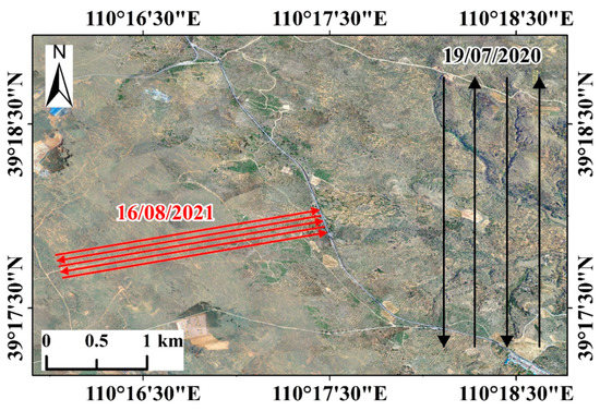
Figure 1.
Geographic location of the study area and schematic flight lines for 19 July 2020 (black) and 16 August 2021 (red).
2.2. Remote Sensing Data
The airborne hyperspectral images were acquired on 19 July 2020 and 16 August 2021 using Wind4 (DJI, Shenzhen, China) equipped with an integrated sensor system. The properties of multi-strip airborne hyperspectral images are listed in Table 1. In this study, the data from 19 July 2020 were utilized to construct the RA-TOC-CA method in Section 3, and the results were analyzed in Section 4. Then, the algorithm was applied to the data on 16 August 2021 to verify the generalizability of the RA-TOC-CA method, with the results shown in Section 4.6. The integrated sensor system consisted of an imaging spectrometer SPECIM FX10 (SPECIM, Oulu, Finland), a control system (DPU), as well as a Global Navigation Satellite System (GNSS) and Inertial Navigation System (INS). The DPU can be used to set flight plans, acquisition frequency, exposure time, and other parameters. The GNSS and INS can record the position and attitude of the imaging spectrometer. The SPECIM FX10 can obtain hyperspectral data with a high signal-to-noise ratio, and it has been commonly used in laboratories and on airborne platforms to collect hyperspectral images. The detailed technical parameters are given in Table 2. The Phantom 4 RTK (DJI, Shenzhen, China) was used to collect digital photos and these photos were used in PhotoScan Pro 1.4.5 (Agisoft, St. Petersburg, Russia) to generate the digital orthophoto map (DOM) and digital elevation model (DEM). The slope and aspect were generated by ArcGIS 10.4.1 (ESRI, Redlands, FL, USA) based on the DEM. Radiometric calibration and geometric correction of hyperspectral images were performed using CaliGeoPro 2.2.4 (SPECIM, Oulu, Finland).

Table 1.
Properties of multi-strip airborne hyperspectral images.
Table 2.
Hyperspectral imager parameters.
3. Methodology
For the main causes of radiation distortion, the method proposed in this paper includes the following three steps: (i) radiation attenuation difference correction, unifying the radiation transmission path of all pixels as the average elevation difference between the UAV and the ground to eliminate the radiation attenuation difference; (ii) topographic correction, combine terrain information, illumination-viewing (sensor’s attitude and IFOV) geometry to construct an improved kernel-driven BRDF model to eliminate the uneven illumination and BRDF effect caused by topography; (iii) consistency adjustment of the multi-strip images, adjust the reflectance according to the fact that homonymous points’ reflectance of adjacent strips should be equal, generate a mosaic result with high radiometric consistency. Figure 2 shows the flowchart of radiation distortion correction for airborne hyperspectral images.
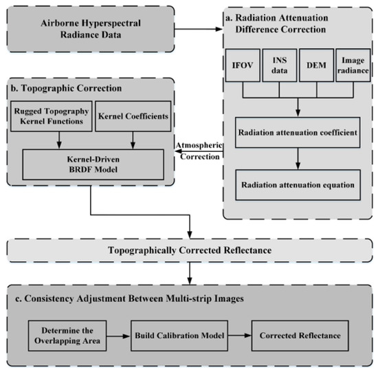
Figure 2.
Processing flowchart of airborne hyperspectral images radiation distortion correction.
3.1. Radiation Attenuation Difference Correction
The IFOV of the push broom imaging spectrometer increases from the scanning center point to the sides, which changes the radiation transmission path and leads to radiation attenuation. According to Bougner’s theorem [37], the radiance after radiation attenuation at the IFOV of is calculated by:
where λ is the wavelength, is the radiance of the ground object, is the radiation transmission path, is the radiation attenuation coefficient, and is the atmospheric thickness.
The radiation attenuation coefficient represents the ratio of radiation energy attenuation over the unit distance, and it is calculated by:
where is the radiation attenuation through , and is the radiation intensity.
Airborne hyperspectral image acquisition is generally performed in a clear and cloudless environment at a low flight altitude. Thus, it can be assumed that the radiation attenuation coefficient is related only to wavelength and atmospheric characteristics, and independent of the pixel’s location [16]. Equation (1) can be simplified as follows:
The radiation transmission path is a function of the viewing geometry, terrain information (slope and aspect), and the elevation difference between the UAV and the ground, and it can be calculated by using Equation (4). The schematic diagram of the viewing geometry is shown in Figure 3.
where is the elevation difference between the UAV and the ground, is the local view zenith angle, is the slope, is the aspect, is the view zenith angle, is the view azimuth angle, is the roll angle, is the IFOV, is the pitch angle, and is the heading angle.
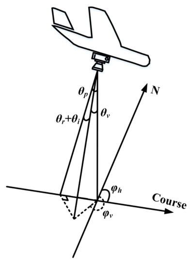
Figure 3.
View zenith angle and view azimuth angle.
According to the assumption of radiation uniformity, the mean ground radiance of each column is equal. Equation (8) represents that the mean ground radiance of the scanning center point was equal to that of other columns.
where m is the number of rows, is the radiance of row j in column i, is the radiation transmission path of row j in column i, is the radiance of row j in the scanning center point, and is the radiation transmission path of row j in the scanning center point.
To avoid the errors caused by the irregular distribution of ground objects and the phenomenon of “the same thing with different radiance”, we constructed the radiance equation group of the scanning center point and other columns and calculated the radiation attenuation coefficient using the least-squares method. Once the radiation attenuation coefficient was obtained, Equation (9) was used to unify the radiation transmission path of all pixels as the average elevation difference between the UAV and the ground to complete the correction of the radiation attenuation difference.
where is the corrected radiance, and is the average elevation difference between the UAV and the ground.
3.2. Topographic Correction
After the radiation attenuation difference correction, the atmospheric correction was performed using the moderate resolution atmospheric transmission (MODTRAN) 5 model to convert the radiance to reflectance. The Mid-Latitude Summer atmospheric model and Rural aerosol model were selected according to the flight date and geographic location. The meteorological parameters were obtained from the local meteorological station. The sensor altitude and ground elevation were obtained from the INS data and DEM, respectively. We, then, used a kernel-driven BRDF approach to eliminate the uneven illumination and BRDF effect caused by topography.
3.2.1. Model Construction and Kernel Selection
The kernel-driven BRDF model decomposes the reflectance into a linear combination of an isotropic kernel, a geometric-optical kernel, and a volumetric scattering kernel. The isotropic kernel represents the radiation fraction without angular dependence, and the geometric-optical kernel describes the geometric structures of the land surface that are not related to wavelength, while the volumetric scattering kernel describes the volumetric scattering effects, which are dependent on the wavelength, with longer wavelengths having stronger scattering power [38,39]. The generic kernel-driven BRDF model is as follows:
where is the isotropic scattering coefficient, and are the volumetric scattering kernel and coefficient, and and are the geometric-optical kernel and coefficient. is the view zenith angle, is the solar zenith angle, is the view azimuth angle, is the solar azimuth angle, is the slope, is the aspect, c is the land-cover type, and λ is the wavelength.
This study used the Li-Transit-Reciprocal (LTR) kernel [40,41] as geometric-optical kernel and the hotspot-revised Ross–Thick–Maignan (RTM) kernel [33,42] as volumetric scattering kernel. The objective of this paper was to construct kernel functions combining terrain, illumination angle, flight attitude, and sensor IFOV. We mainly introduce using Equations (6) and (7) to calculate the view zenith angle and the view azimuth angle.
where is the local solar zenith angle, is the local view zenith angle, is the solar azimuth angle, is the view azimuth angle, is the solar zenith angle, is the slope, and is the aspect. A constant value of = 1.5° is used to indicate the half-width of the hotspot for most of the targets [42]. The relative canopy height h/b is set to 2 for trees and shrubs, and 1 for grass. The relative canopy shape b/r is set to 1 for all land-cover types.
3.2.2. Kernel Coefficients Determination
Accurate calculation of kernel coefficients is a key step in building the BRDF model. Previous studies demonstrated that terrestrial reflectance anisotropy varies with the land cover type [13,43,44,45], and the estimation of coefficients based on the stratification of the surface is a good choice [39,46]. Therefore, we used the random forest (RF) method to classify the whole set of images into four types: herb, shrub, tree, and bare soil and established a classification-based BRDF model.
The stratified sampling method [33] was used to obtain the number of pixels to fit the kernel coefficients, and the specific steps followed were as follows:
(1) n took any values between 1000 and 10,000, with a step length of 100 pixels (i.e., 1000, 1100, …, 9900, 10,000); for each land type, calculated the cos(i) of all pixels and arranged them in ascending order, extracted n pixels at equal intervals from the sorted sequence;
(2) Based on the reflectance and kernel functions of the selected pixels in step (1), the kernel coefficients of different land types were fitted using the least-squares method;
(3) The RMSE between the fitted reflectance and the image reflectance was calculated, and the coefficients corresponding to the smallest RMSE were selected as the optimal kernel coefficients.
As shown in Figure 4, the RMSE value on the same band did not change significantly with the sample number. The kernel coefficients corresponding to the minimum RMSE were selected for a subsequent correction.
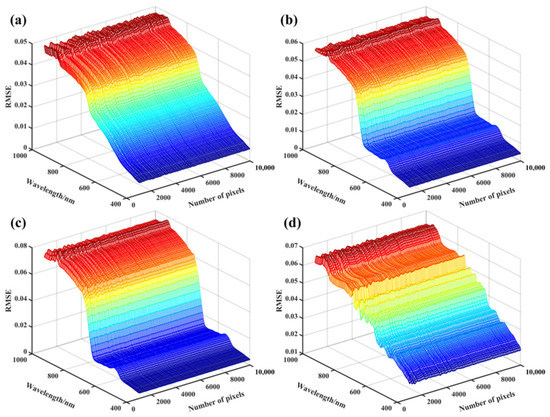
Figure 4.
The RMSE of fitted reflectance with different sample numbers. (a) herb, (b) shrub, (c) tree, (d) bare soil.
3.2.3. Angle Normalization
Calculate the ratio of the simulated reflectance at the reference geometry (nadir view, flat topography, mean solar angles for all strips) to the simulated reflectance at the observed geometry [47], and then multiply the image’s original reflectance by this ratio to obtain the topographically corrected reflectance.
where is the topographically corrected reflectance, is the image’s original reflectance, is the simulated reflectance at the observed geometry, is the simulated reflectance at the reference geometry, is the mean solar zenith angle for all strips, and is the mean solar azimuth angle for all strips.
3.3. Consistency Adjustment between Multi-Strip Images
After the topographic correction, adjacent images may still have radiation differences due to differences in multi-strip images acquisition time, meteorological conditions, and other factors. According to the fact that the reflectance of homonymous points in adjacent images should be equal, the reflectance was adjusted by:
where and are the reflectance before and after correction, respectively, and a and b are correction coefficients.
The reflectance difference of the homonymous points between adjacent images after correction should be the smallest. That is, the difference of the mean value and the standard deviation between the adjacent image overlapping areas is the smallest, which can be expressed by Equations (25) and (26).
where is the difference of the mean value between the ith and jth strips after correction, is the difference of the standard deviation between the ith and jth strips after correction, and are correction coefficients for the ith strip, and are correction coefficients for the jth strip, and are the mean value and standard deviation of the ith strip, respectively, and and are the mean value and standard deviation of the jth strip, respectively.
In addition, the difference of the mean value and standard deviation of images before and after correction should be minimal, which can be expressed by Equations (27) and (28).
where is the difference between the mean value before and after correction of the ith strip, and is the difference between the standard deviation before and after correction of the ith strip.
The error equations for all strips are shown in Equation (29), and the least-squares method was used to calculate the correction coefficients. After obtaining the correction coefficients of each strip, the hyperspectral images with consistent radiation can be obtained through Equation (24).
3.4. Correction Effect Evaluation
To evaluate the effectiveness of the proposed RA-TOC-CA method, the RA-TOC-CA and two other methods (i.e., SCS+C and Minnaert+SCS, see Table 3) were used to correct the radiation distortion of hyperspectral images. The correction effects of different methods were assessed through visual inspection and quantitative indicators.
Table 3.
Expressions of the methods for comparison.
(1) The mean radiance of each scanning column before and after the correction of the radiation attenuation difference was calculated. An ideal correction method should reduce the differences in the mean radiance of different columns [16].
(2) Visual inspection checked if the reflectance difference between sunny and shady slopes and chromatic aberration of the mosaicked data are weakened.
(3) The linear relationship between the cos(i) and the reflectance and the mean reflectance between different aspects were analyzed. An effective correction method should result in the R2 values between the cos(i) and the reflectance to zero [48] and reduce the reflectance difference between different aspects [49].
(4) The reflectance difference of homonymous points and the brightness gradient between adjacent images were analyzed. An effective correction method should reduce the reflectance difference and brightness gradient [33].
(5) The correlation between the airborne image spectra and the ground spectra was analyzed. The handheld hyperspectral camera SPECIM IQ (SPECIM, Oulu, Finland) was used to collect the ground spectra data. The results of an effective correction should show a high correlation with the ground spectra [50].
(6) The generalizability of the proposed method was verified. An effective method can be extended to different airborne hyperspectral images to eliminate radiation distortion [33].
4. Results
4.1. Effects of Radiation Attenuation Difference Correction
This section compares the radiance curves before and after the correction of the radiation attenuation difference. Since the comparison methods SCS+C and Minnaert+SCS are used to correct the image reflectance, they are not used in this part. The results of all bands are similar, and the sky diffuse radiation in the near infrared band (834.83 nm) is small [20,53], which has a more remarkable effect. The following is an example of this band to show the radiation distortion correction effects. The mean radiance of each scanning column before and after the correction of the radiation attenuation difference was calculated, as shown in Figure 5. Due to different radiation transmission paths, the uncorrected image showed a decreasing trend from the center to the edge. The standard deviation between the mean radiance of each column was 186.56 W/cm2/sr/μm. After correction, the difference between the mean radiance of each column decreased and the standard deviation was reduced to 82.02 W/cm2/sr/μm. There were still differences in the corrected mean radiance, mainly due to the following two points: the distribution of ground objects between different columns was not completely consistent, and the components of the same objects at various locations are different, resulting in different radiance.
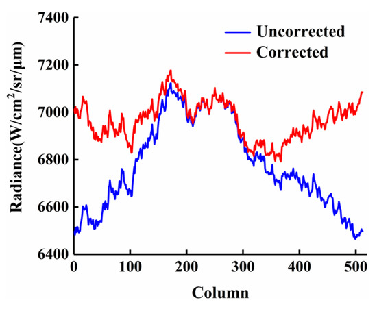
Figure 5.
Comparison of radiance before and after correction for radiation attenuation difference.
4.2. Visual Inspection of Radiation Distortion Correction
The outline, seamline, and true color composite images of the hyperspectral mosaic data are presented in Figure 6. The reflectance in the uncorrected image was significantly affected by topographic effects, i.e., shaded areas were darker than illuminated areas. In addition, there were obvious cross-track brightness gradients in the uncorrected hyperspectral image, which destroyed the integrity of the mosaic result. It can be noticed that SCS+C and Minnaert+SCS weakened the topographic effect, but there was still a brightness gradient between adjacent images. The SCS+C image became too bright in some shaded areas, indicating that the reflectance was overcorrected. Although the RA-TOC-CA corrected image still has a certain topographic effect, the algorithm eliminated the brightness mismatch at the image’s edge and realized the seamless mosaicking of multiple flight strips.
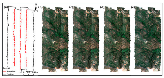
Figure 6.
True color composite images before and after correction. (a) Outline and seamline of the hyperspectral mosaic image, (b) Uncorrected mosaic, (c) SCS+C corrected mosaic, (d) Minnaert+SCS corrected mosaic, (e) RA-TOC-CA corrected mosaic.
4.3. Effects of Topographic Correction
4.3.1. Correlation Analysis of Reflectance and Cosine of the Local Solar Incidence Angle
This section compares the relationship between cos(i) and reflectance corrected by different methods. The relationship between the reflectance at 834.83 nm and the cos(i) is shown in Figure 7. There was a positive linear relationship between the uncorrected reflectance and cos(i); for the herb, shrub, tree, and bare soil, the R2 values were 0.1235, 0.1538, 0.1313, and 0.1163, respectively. The correlations decreased after using the three methods, indicating that the influence of illumination conditions was weakened. RA-TOC-CA achieved the best results for each land type (the R2 values of the herb, shrub, tree, and bare soil were 0.0031, 0.0051, 0.0001, and 0.0212, respectively). However, the slope of herb, shrub, and tree turned negative after SCS+C correction, while the slope of shrub after RA-TOC-CA correction also became negative, indicating that the reflectance was overcorrected. The overcorrection of SCS+C is consistent with other studies [54,55]. Unlike the strategy that relies on the regression relationship between the reflectance and illumination conditions [56,57], RA-TOC-CA not only considers the illumination geometry but also the viewing geometry (sensor’s attitude and IFOV), which has a more complete physical mechanism.
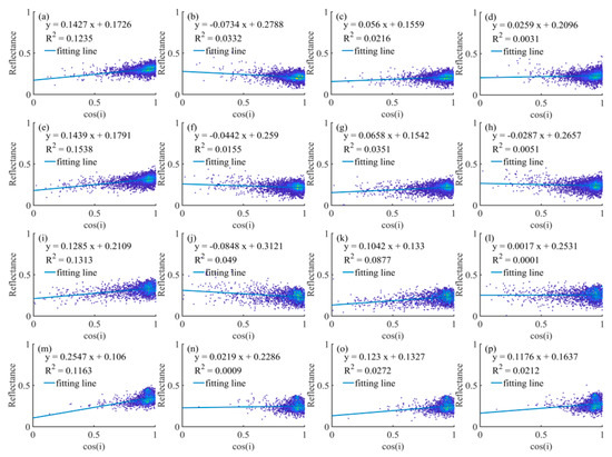
Figure 7.
Density scatterplots between the reflectance of herb (a–d), shrub (e–h), tree (i–l), and bare soil (m–p) at 834.83 nm and the cosine of the local solar incidence angle (cos(i)). (a) Uncorrected, (b) SCS+C, (c) Minnaert+SCS, (d) RA-TOC-CA; (e) Uncorrected, (f) SCS+C, (g) Minnaert+SCS, (h) RA-TOC-CA; (i) Uncorrected, (j) SCS+C, (k) Minnaert+SCS, (l) RA-TOC-CA; (m) Uncorrected, (n) SCS+C, (o) Minnaert+SCS, (p) RA-TOC-CA.
4.3.2. Reflectance of Different Aspects
The aspect was divided into steps of 15°, and the mean reflectance was calculated in different intervals, as shown in Figure 8. In the uncorrected image, the reflectance over the sun-facing aspects was remarkably larger than those in the opposite directions. Compared with the uncorrected image, SCS+C showed the opposite trend. That is, the reflectance of the shady aspect was larger than that of the sunny aspect, which indicates that SCS+C overcorrected the reflectance. After Minnaert+SCS and RA-TOC-CA correction, the reflectance difference decreased significantly over each aspect. However, the area of the RA-TOC-CA-derived circle was larger than the uncorrected image, which indicated that the corrected reflectance increased as a whole. This was because the radiance increased after reducing the radiation attenuation difference and the reflectance value increased after atmospheric correction.
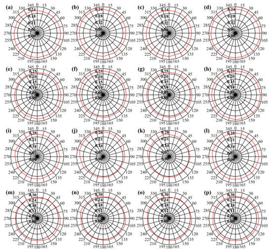
Figure 8.
The average reflectance of herb (a–d), shrub (e–h), tree (i–l), and bare soil (m–p) in different aspects. The radius represents the magnitude of the reflectance with zero in the center, and the polar angle represents the aspect. (a) Uncorrected, (b) SCS+C, (c) Minnaert+SCS, (d) RA-TOC-CA; (e) Uncorrected, (f) SCS+C, (g) Minnaert+SCS, (h) RA-TOC-CA; (i) Uncorrected, (j) SCS+C, (k) Minnaert+SCS, (l) RA-TOC-CA; (m) Uncorrected, (n) SCS+C, (o) Minnaert+SCS, (p) RA-TOC-CA.
To quantitatively analyze the reflectance distribution, the coefficient of variation (CV) of the reflectance across different aspects is listed in Table 4. Minnaert+SCS performed the best in the shrub (1.24%). For the herb, tree, and bare soil, RA-TOC-CA had the lowest CV (1.44%, 1.54%, and 1.57%, respectively).
Table 4.
The coefficient of variation (%) of reflectance across different aspects.
4.4. Analysis of Overlapping Areas of Adjacent Flight Strips
We first evaluated the reflectance difference of the homonymous points between adjacent strips through visual inspection and then assessed the reflectance difference using the quantitative indicator. An example of the reflectance curves of the homonymous points in the adjacent images is shown in Figure 9. The reflectance of strip B was significantly higher than that of strip A before correction, more significant in the near infrared band (>700 nm). The effect of the three correction methods was Minnaert+SCS, SCS+C, and RA-TOC-CA, from inferior to superior. In particular, the reflectance curves almost coincide in the partial spectral range after RA-TOC-CA correction. The RMSE of the homonymous points’ reflectance in the adjacent images is shown in Figure 10. Compared with the uncorrected spectrum, all three methods reduce the RMSE, especially in the near infrared band, implying that the adjacent images had more similar spectral values in the overlapping area. RA-TOC-CA resulted in the lowest RMSE, compared with the uncorrected image, the RMSE of the herb, shrub, tree, and bare soil decreased by 33.57%, 27.76%, 14.40%, and 36.35% on average, respectively.
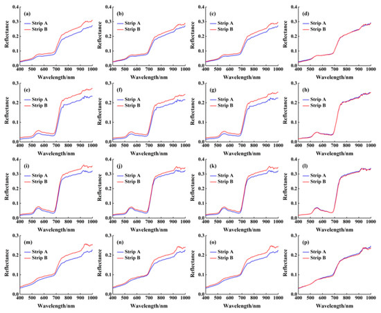
Figure 9.
An example of the reflectance curves of the homonymous points for herb (a–d), shrub (e–h), tree (i–l), and bare soil (m–p) in the adjacent images. (a) Uncorrected, (b) SCS+C, (c) Minnaert+SCS, (d) RA-TOC-CA; (e) Uncorrected, (f) SCS+C, (g) Minnaert+SCS, (h) RA-TOC-CA; (i) Uncorrected, (j) SCS+C, (k) Minnaert+SCS, (l) RA-TOC-CA; (m) Uncorrected, (n) SCS+C, (o) Minnaert+SCS, (p) RA-TOC-CA.
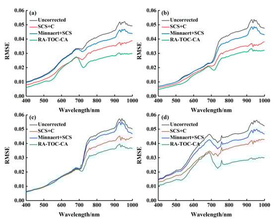
Figure 10.
RMSE of the homonymous points’ reflectance in the adjacent images before and after correction. (a) herb, (b) shrub, (c) tree, (d) bare soil.
We also calculate the transition from one strip to another. The specific procedure was as follows: The two right-most strips, denoted as strips A and B, were selected; the seamline of the mosaic image is presented in Figure 11. Next, 50 columns from the seamline to the left were selected as the reflectance of strip A, and 50 columns to the right were selected as the reflectance of strip B. After removing the non-vegetated area, the mean reflectance of each column was calculated (Figure 12). The uncorrected reflectance increased sharply at the abscissa of zero, which indicated that there is a brightness mismatch at the edge of adjacent images. SCS+C and Minnaert+SCS reduced the two strips’ difference, but the effect was not significant, and the reflectance of these two methods showed an overall increase and decrease trend, respectively, compared with the uncorrected image. The gradient of the RA-TOC-CA corrected reflectance at the abscissa of zero declined, and the integrity was better.
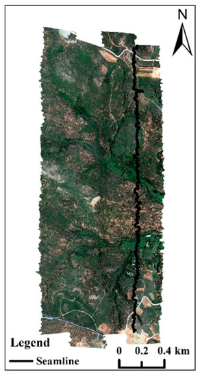
Figure 11.
Schematic diagram of the seamline.
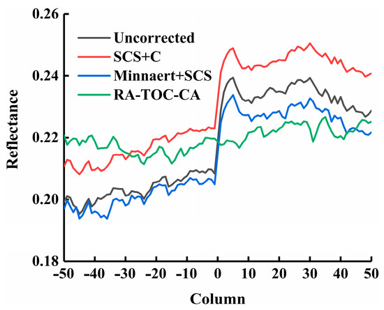
Figure 12.
Transitions at the edges of hyperspectral images. The negative semi-axis of the horizontal axis represents the columns of strip A, and the positive semi-axis represents the columns of strip B. The smaller the absolute value of the coordinate, the closer to the seamline.
4.5. Reflectance Comparison between the Image and the Ground Spectra
An example of the reflectance of the image and the ground spectra is shown in Figure 13. The shapes of the two reflectance curves were similar, but there were significant differences in the values. The image spectra were the absolute reflectance obtained by the atmospheric correction, while the ground spectra were the relative reflectance. Moreover, the spectral response functions of the two sensors were different, as was their sensitivity to ground objects. Accordingly, the reflectance of the same ground objects obtained by two sensors was different to a certain extent. The reflectance comparison between the image and ground spectra at 834.83 nm is shown in Table 5. There was a high linear relationship between the image and the ground reflectance. Compared with the uncorrected image, R2 of SCS+C and Minnaert+SCS decreased, whereas RA-TOC-CA achieved the highest correlation.
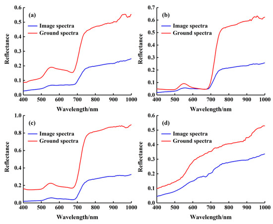
Figure 13.
An example of the reflectance of the image and the ground spectra. (a) herb, (b) shrub, (c) tree, (d) bare soil.
Table 5.
The regression results between the image spectra (y) and the ground spectra (x) at 834.83 nm.
4.6. The Generalizability of RA-TOC-CA
To verify the generalization ability of the proposed algorithm, the RA-TOC-CA method was applied to the airborne hyperspectral images collected on 16 August 2021. The comparison between uncorrected and corrected images is presented in Figure 14. There were clear cross-track brightness gradients in the uncorrected image, while these gradients were almost absent in the image corrected by the RA-TOC-CA method. This demonstrates that the RA-TOC-CA method has good generalization ability and can correct the radiation distortion of different hyperspectral images.
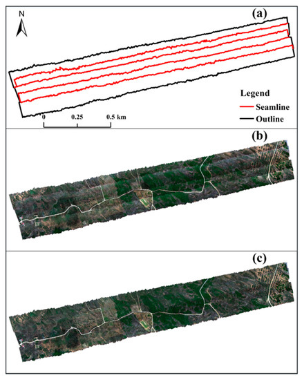
Figure 14.
True color composite images of airborne hyperspectral data collected on 16 August 2021 before and after correction. (a) Outline and seamline of the hyperspectral mosaic image, (b) Uncorrected mosaic, (c) RA-TOC-CA corrected mosaic.
5. Discussion
5.1. Comparison of Different Methods
In addition to the proposed RA-TOC-CA method, the SCS+C and Minnaert+SCS methods were used in the comparison tests, which have been proven to be effective in eliminating the terrain effect [58,59,60,61]. The experimental results showed that both SCS+C and Minnaert+SCS weakened the topographic effect, but SCS+C overcorrected the original image, and there were still cross-track brightness gradients in the two correction data. SCS+C has been developed based on the Lambertian hypothesis [62]. This approach was constructed under the assumption of dense vegetation with a continuous canopy and implements the topographic correction by normalizing the sunlit canopy area. SCS+C neglects the volume scattering of leaves within the canopy. When the canopy area is larger than a pixel or the canopy is shaded within the pixel, SCS+C cannot eliminate the effects caused by surrounding terrain or canopy shading [63]. Moreover, SCS+C ignores the BRDF distortion caused by surface orientations [62]. Minnaert+SCS was based on the non-Lambertian hypothesis, and the influence of the BRDF was added to the correction process; namely, parameter k was used to indicate the degree of bidirectional reflection [63]. However, Minnaert+SCS only considered direct solar radiation, not diffuse reflection and surrounding terrain radiation [23]. Therefore, the correction effect of these two methods is not ideal. RA-TOC-CA was based on the radiation transfer process, not only considering the illumination-viewing geometry but also eliminating the radiation attenuation difference caused by the wide field of view and adjusting the reflectance of multi-strip images as a whole. The proposed method has certain deficiencies in eliminating the radiation difference between sunlit and shaded, which are clearly visible in the true color composite image. Nevertheless, RA-TOC-CA reduces the BRDF effect and brightness gradient and obtains an image with good radiometric consistency.
5.2. Physical Soundness Analysis
When the solar and viewing directions are perpendicular to the aspect, the slope does not influence the reflectance. That is, the reflectance does not change before and after terrain correction under these geometric conditions [48]. To analyze the correction methods’ physical soundness, the density scatterplots between the uncorrected and corrected reflectance at 834.83 nm over aspects perpendicular to the solar and viewing directions are presented in Figure 15. The fitting results of the same correction method for different land types were similar. The points in the SCS+C-derived scatterplot were clustered around the 1:1 line, but they showed a slight shift to high values, indicating that the reflectance was overestimated by the SCS+C method. The Minnaert+SCS-derived reflectance showed an opposite trend to that of SCS+C, i.e., the fitting line shifted to low values, revealing that the reflectance was under-corrected by this method, which was consistent with the conclusion in Section 4.4. RA-TOC-CA had the highest R2, but the RMSE of shrub was higher than SCS+C and that of bare soil was higher than Minnaert+SCS. RA-TOC-CA had the largest Bias, revealing a systematically positive shift in reflectance. This is because the radiance value increased when the radiation attenuation difference was eliminated, and the reflectance value after atmospheric correction increased accordingly. These results showed that the RA-TOC-CA method corrects hyperspectral data on a physical level and avoids the appearance of unreasonable correction results.
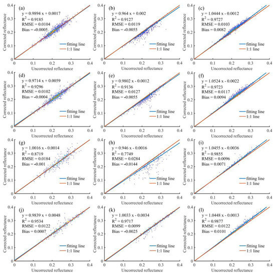
Figure 15.
Density scatterplots between the corrected and original reflectance of herb (a–c), shrub (d–f), tree (g–i), and bare soil (j–l) over aspects perpendicular to the solar and viewing directions. (a) SCS+C, (b) Minnaert+SCS, (c) RA-TOC-CA; (d) SCS+C, (e) Minnaert+SCS, (f) RA-TOC-CA; (g) SCS+C, (h) Minnaert+SCS, (i) RA-TOC-CA; (j) SCS+C, (k) Minnaert+SCS, (l) RA-TOC-CA.
5.3. Future Work
In the final step of eliminating radiation distortion, the correction coefficients are calculated by the error equation that the reflectance of the adjacent strips’ homonymous points should be equal. The relative reflectance between different strips is good, but there is no certain physical basis for the solution of absolute reflectance. In the future, a radiometric correction method with more complete physical characteristics will be studied.
In addition, the proposed elimination method for the radiation attenuation difference is based on the assumption of radiation uniformity. Although the proposed method can achieve good results for evenly-distributed ground objects, its correction effect could decay when the ground objects change considerably. As explained before, the proposed RA-TOC-CA method first eliminates the radiation attenuation difference and then removes the topographic effect. The topography affects the radiance of hyperspectral data. In the future, methods for eliminating the effects of radiation attenuation and topography simultaneously will be studied.
6. Conclusions
In this paper, we presented a comprehensive method for correcting the radiation distortion of airborne hyperspectral images (RA-TOC-CA). The RA-TOC-CA method is based on multi-angular scanning and takes into account the topography, illumination-viewing geometry, and radiation differences between multiple strips, which has a complete theoretical basis. The proposed method was compared with the other two methods (SCS+C and Minnaert+SCS) in correcting the radiation distortion of airborne hyperspectral images. In general, all three methods weakened the topographic effects, but the images corrected by SCS+C and Minnaert+SCS still had cross-track brightness gradients, and SCS+C overcorrected the reflectance. The RA-TOC-CA method not only had the best visual effect but also outperformed the other two methods in quantitative assessment. RA-TOC-CA provides an effective approach to reducing radiation attenuation difference, topographic effects, and radiation differences between multiple strips, and facilitates the generation of high-quality hyperspectral data.
Author Contributions
Conceptualization, Y.Z.; Formal analysis, Y.Z.; Funding acquisition, S.L.; Investigation, Y.Z., Y.T., Y.L., X.H., D.G., C.J.; Methodology, Y.Z.; Project administration, S.L.; Supervision, S.L.; Validation, S.L.; Writing—original draft, Y.Z.; Writing—review and editing, S.L. All authors have read and agreed to the published version of the manuscript.
Funding
This research was funded by Green exploitation of coal resources and its environmental effects in Xinjiang (U1903209).
Data Availability Statement
The data supporting the findings of this study are available from the corresponding author on request.
Acknowledgments
We would like to thank Yangnan Guo and Kunlei Wang for their help in the process of data collection. The authors greatly appreciate the anonymous reviewers’ excellent comments in improving the manuscript’s quality.
Conflicts of Interest
The authors declare no conflict of interest.
References
- Wang, X.; Tan, K.; Du, Q.; Chen, Y.; Du, P. Caps-TripleGAN: GAN-Assisted CapsNet for Hyperspectral Image Classification. IEEE Trans. Geosci. Remote Sens. 2019, 57, 7232–7245. [Google Scholar] [CrossRef]
- Zhang, C.; Han, M. Multi-feature hyperspectral image classification with L 2,1 norm constrained joint sparse representation. Int. J. Remote Sens. 2021, 42, 4785–4804. [Google Scholar] [CrossRef]
- Myr, J.; Keski-Saari, S.; Kivinen, S.; Tanh Ua Np, T.; Vihervaara, P. Tree species classification from airborne hyperspectral and LiDAR data using 3D convolutional neural networks. Remote Sens. Environ. 2021, 256, 112322. [Google Scholar] [CrossRef]
- Shi, T.; Chen, Y.; Liu, Y.; Wu, G. Visible and near-infrared reflectance spectroscopy-An alternative for monitoring soil contamination by heavy metals. J. Hazard. Mater. 2014, 265, 166–176. [Google Scholar] [CrossRef]
- Liu, P.; Liu, Z.; Hu, Y.; Shi, Z.; Pan, Y.; Wang, L.; Wang, G. Integrating a Hybrid Back Propagation Neural Network and Particle Swarm Optimization for Estimating Soil Heavy Metal Contents Using Hyperspectral Data. Sustainability 2019, 11, 419. [Google Scholar] [CrossRef]
- Liu, Z.; Lu, Y.; Peng, Y.; Zhao, L.; Hu, Y. Estimation of Soil Heavy Metal Content Using Hyperspectral Data. Remote Sens. 2019, 11, 1464. [Google Scholar] [CrossRef]
- Tan, K.; Wang, H.; Chen, L.; Du, Q.; Du, P.; Pan, C. Estimation of the spatial distribution of heavy metal in agricultural soils using airborne hyperspectral imaging and random forest. J. Hazard. Mater. 2020, 382, 120987. [Google Scholar] [CrossRef]
- Landmann, T.; Piiroinen, R.; Makori, D.M.; Abdel-Rahman, E.M.; Makau, S.; Pellikka, P.; Raina, S.K. Application of hyperspectral remote sensing for flower mapping in African savannas. Remote Sens. Environ. 2015, 166, 50–60. [Google Scholar] [CrossRef]
- Roth, K.L.; Roberts, D.A.; Dennison, P.E.; Alonzo, M.; Beland, M. Differentiating plant species within and across diverse ecosystems with imaging spectroscopy. Remote Sens. Environ. 2015, 167, 135–151. [Google Scholar] [CrossRef]
- Hakkenberg, C.; Peet, R.; Urban, D.; Song, C. Modeling plant composition as community continua in a forest landscape with LiDAR and hyperspectral remote sensing. Ecol. Appl. 2017, 28, 177–190. [Google Scholar] [CrossRef]
- Schiefer, S.; Hostert, P.; Damm, A. Correcting brightness gradients in hyperspectral data from urban areas. Remote Sens. Environ. 2006, 101, 25–37. [Google Scholar] [CrossRef]
- Köppl, C.J.; Malureanu, R.; Dam-Hansen, C.; Wang, S.; Jin, H.; Barchiesi, S.; Sandí, J.M.S.; Munoz-Carpena, R.; Johnson, M.; Durán-Quesada, A.M. Hyperspectral reflectance measurements from UAS under intermittent clouds: Correcting irradiance measurements for sensor tilt. Remote Sens. Environ. 2021, 267, 112719. [Google Scholar] [CrossRef]
- Jensen, D.J.; Simard, M.; Cavanaugh, K.C.; Thompson, D.R. Imaging spectroscopy BRDF correction for mapping Louisiana’s coastal ecosystems. IEEE Trans. Geosci. Remote Sens. 2017, 56, 1739–1748. [Google Scholar] [CrossRef]
- Schläpfer, D.; Richter, R.; Feingersh, T. Operational BRDF effects correction for wide-field-of-view optical scanners (BREFCOR). IEEE Trans. Geosci. Remote Sens. 2014, 53, 1855–1864. [Google Scholar] [CrossRef]
- Guo, X.; Wang, R. Radiometric Correction of Airborne Imaging Spectrometer Data. J. Image Graph. 2000, 5, 19–23. [Google Scholar]
- Tian, Y.; Wu, W.; Yang, G. Edge radiation distortion correction of whiskbroom airborne hyperspectral image by considering BRDF effect and atmospheric attenuation. J. Infrared Millim. Waves. 2016, 35, 701–707. [Google Scholar]
- Horvath, R.; Braithwaite, J.G.; Polcyn, F.C. Effects of atmospheric path on airborne multispectral sensors. Remote Sens. Environ. 1970, 1, 203–215. [Google Scholar] [CrossRef]
- Stokkom, H.V.; Guzzi, R. Atmospheric spectral attenuation of airborne remote-sensing data Comparison between experimental and theoretical approach. Int. J. Remote Sens. 1984, 5, 925–938. [Google Scholar] [CrossRef]
- Li, F.; Jupp, D.; Thankappan, M.; Lymburner, L.; Mueller, N.; Lewis, A.; Held, A. A physics-based atmospheric and BRDF correction for Landsat data over mountainous terrain. Remote Sens. Environ. 2012, 124, 756–770. [Google Scholar] [CrossRef]
- Li, A.; Wang, Q.; Bian, J.; Lei, G. An Improved Physics-Based Model for Topographic Correction of Landsat TM Images. Remote Sens. 2015, 7, 6296–6319. [Google Scholar] [CrossRef]
- Flood, N.; Danaher, T.; Gill, T.; Gillingham, S. An Operational Scheme for Deriving Standardised Surface Reflectance from Landsat TM/ETM+ and SPOT HRG Imagery for Eastern Australia. Remote Sens. 2013, 5, 83–109. [Google Scholar] [CrossRef]
- Schaaf, C.B.; Li, X.; Strahler, A.H. Topographic effects on bidirectional and hemispherical reflectances calculated with a geometric-optical canopy model. IEEE Trans. Geosci. Remote Sens. 2002, 32, 1186–1193. [Google Scholar] [CrossRef]
- Gao, Y.; Zhang, W. A simple empirical topographic correction method for ETM+ imagery. Int. J. Remote Sens. 2009, 30, 2259–2275. [Google Scholar] [CrossRef]
- Jiang, K.; Hu, C.; Yu, K.; Zhao, Y. Landsat TM/ETM + topographic correction method based on smoothed terrain and semi-empirical model. J. Remote Sens. 2014, 18, 287–306. [Google Scholar]
- Lin, Q.; Huang, H.; Chen, L.; Chen, E. Topographic correction method for steep mountain terrain images. J. Remote Sens. 2017, 21, 776–784. [Google Scholar]
- Zhang, Y.; Li, X.; Wen, J.; Liu, Q.; Yan, G. Improved Topographic Normalization for Landsat TM Images by Introducing the MODIS Surface BRDF. Remote Sens. 2015, 7, 6558–6575. [Google Scholar] [CrossRef]
- Sandmeier, S.; Itten, K.I. A physically-based model to correct atmospheric and illumination effects in optical satellite data of rugged terrain. IEEE Trans. Geosci. Remote Sens. 1997, 35, 708–717. [Google Scholar] [CrossRef]
- Zhang, Z.; He, G.; Liu, D.; Wang, X.; Jiang, H. An Improved Physical Model to Correct Topographic Effects in Remotely Sensed Imagery. Spectrosc. Spectr. Anal. 2010, 30, 1839–1842. [Google Scholar]
- Collings, S.; Caccetta, P.; Campbell, N.; Wu, X. Techniques for BRDF Correction of Hyperspectral Mosaics. IEEE Trans. Geosci. Remote Sens. 2010, 48, 3733–3746. [Google Scholar] [CrossRef]
- Jiao, Z.; Dong, Y.; Schaaf, C.B.; Chen, J.M.; Román, M.; Wang, Z.; Zhang, H.; Ding, A.; Erb, A.; Hill, M.J.; et al. An algorithm for the retrieval of the clumping index (CI) from the MODIS BRDF product using an adjusted version of the kernel-driven BRDF model. Remote Sens. Environ. 2018, 209, 594–611. [Google Scholar] [CrossRef]
- Roujean, J.L.; Leroy, M.; Deschamps, P.Y. A bidirectional reflectance model of the Earth’s surface for the correction of remote sensing data. J. Geophys. Res. Atmos. 1992, 97, 20455–20468. [Google Scholar] [CrossRef]
- Wang, Z.; Liu, L. Correcting Bidirectional Effect for Multiple-Flightline Aerial Images Using a Semiempirical Kernel-Based Model. IEEE J. Sel. Top. Appl. Earth Obs. Remote Sens. 2016, 9, 4450–4463. [Google Scholar] [CrossRef]
- Jia, W.; Pang, Y.; Tortini, R.; Schläpfer, D.; Li, Z.; Roujean, J.-L. A Kernel-Driven BRDF Approach to Correct Airborne Hyperspectral Imagery over Forested Areas with Rugged Topography. Remote Sens. 2020, 12, 432. [Google Scholar] [CrossRef]
- Queally, N.; Ye, Z.; Zheng, T.; Chlus, A.; Schneider, F.; Pavlick, R.P.; Townsend, P.A. FlexBRDF: A flexible BRDF correction for grouped processing of airborne imaging spectroscopy flightlines. J. Geophys. Res. 2022, 127, e2021JG006622. [Google Scholar] [CrossRef] [PubMed]
- Kizel, F.; Benediktsson, J.A.; Bruzzone, L.; Pedersen, G.B.; Vilmundardóttir, O.K.; Falco, N. Simultaneous and constrained calibration of multiple hyperspectral images through a new generalized empirical line model. IEEE J. Sel. Top. Appl. Earth Obs. Remote Sens. 2018, 11, 2047–2058. [Google Scholar] [CrossRef]
- Li, D.; Wang, M.; Pan, J. Auto-dodging Processing and Its Application for Optical RS Images. Geomat. Inf. Sci. Wuhan Univ. 2006, 31, 753–756. [Google Scholar]
- Patterson, E.M.; Gillette, D.A.; Stockton, B.H. Complex index of refraction between 300 and 700 nm for Saharan aerosols. J. Geophys. Res. 1977, 82, 3153–3160. [Google Scholar] [CrossRef]
- Weyermann, J.; Kneubuhler, M.; Schlapfer, D.; Schaepman, M.E. Minimizing Reflectance Anisotropy Effects in Airborne Spectroscopy Data Using Ross–Li Model Inversion with Continuous Field Land Cover Stratification. IEEE Trans. Geosci. Remote Sens. 2015, 53, 5814–5823. [Google Scholar] [CrossRef]
- Guo, Y.; Jia, X.; Paull, D. Superpixel-based adaptive kernel selection for angular effect normalization of remote sensing images with kernel learning. IEEE Trans. Geosci. Remote Sens. 2017, 55, 4262–4271. [Google Scholar] [CrossRef]
- Li, X.; Gao, F.; Chen, L.; Strahler, A.H. Derivation and validation of a new kernel for kernel-driven BRDF models. Remote. Sens. Earth Sci. Ocean. Sea Ice Appl. 1999, 3868, 368–379. [Google Scholar]
- Zhang, X.; Jiao, Z.; Dong, Y.; Zhang, H.; Li, Y.; He, D.; Ding, A.; Yin, S.; Cui, L.; Chang, Y. Potential Investigation of Linking PROSAIL with the Ross-Li BRDF Model for Vegetation Characterization. Remote Sens. 2018, 10, 437. [Google Scholar] [CrossRef]
- Maignan, F.; Bréon, F.M.; Lacaze, R. Bidirectional reflectance of Earth targets: Evaluation of analytical models using a large set of spaceborne measurements with emphasis on the Hot Spot. Remote Sens. Environ. 2004, 90, 210–220. [Google Scholar] [CrossRef]
- Roy, D.P.; Zhang, H.K.; Ju, J.; Gomez-Dans, J.L.; Lewis, P.E.; Schaaf, C.B.; Sun, Q.; Li, J.; Huang, H.; Kovalskyy, V. A general method to normalize Landsat reflectance data to nadir BRDF adjusted reflectance. Remote Sens. Environ. 2016, 176, 255–271. [Google Scholar] [CrossRef]
- Gatebe, C.K.; King, M.D. Airborne spectral BRDF of various surface types (ocean, vegetation, snow, desert, wetlands, cloud decks, smoke layers) for remote sensing applications. Remote Sens. Environ. 2016, 179, 131–148. [Google Scholar] [CrossRef]
- Mira, M.; Weiss, M.; Baret, F.; Courault, D.; Hagolle, O.; Gallego-Elvira, B.; Olioso, A. The MODIS (collection V006) BRDF/albedo product MCD43D: Temporal course evaluated over agricultural landscape. Remote Sens. Environ. 2015, 170, 216–228. [Google Scholar] [CrossRef]
- Luo, Y. Surface bidirectional reflectance and albedo properties derived using a landcover based approach with MODIS observations. J. Geophys. Res. 2005, 110, D1106. [Google Scholar] [CrossRef]
- Colgan, M.S.; Baldeck, C.A.; Féret, J.; Asner, G.P. Mapping savanna tree species at ecosystem scales using support vector machine classification and BRDF correction on airborne hyperspectral and LiDAR data. Remote Sens. 2012, 4, 3462–3480. [Google Scholar] [CrossRef]
- Yin, G.; Li, A.; Zhao, W.; Jin, H.; Bian, J. Modeling Canopy Reflectance Over Sloping Terrain Based on Path Length Correction. IEEE Trans. Geosci. Remote Sens. 2017, 55, 4597–4609. [Google Scholar] [CrossRef]
- Balthazar, V.; Vanacker, V.; Lambin, E.F. Evaluation and parameterization of ATCOR3 topographic correction method for forest cover mapping in mountain areas. Int. J. Appl. Earth Obs. Geoinf. 2012, 18, 436–450. [Google Scholar] [CrossRef]
- Tan, K.; Niu, C.; Jia, X.; Ou, D.; Lei, S. Complete and accurate data correction for seamless mosaicking of airborne hyperspectral images: A case study at a mining site in Inner Mongolia, China. ISPRS J. Photogramm. Remote Sens. 2020, 165, 1–15. [Google Scholar] [CrossRef]
- Soenen, S.A.; Peddle, D.R.; Coburn, C.A. SCS+ C: A modified sun-canopy-sensor topographic correction in forested terrain. IEEE Trans. Geosci. Remote Sens. 2005, 43, 2148–2159. [Google Scholar] [CrossRef]
- Reeder, D.H. Topographic Correction of Satellite Images: Theory and Application; Dartmouth College: Hanover, NH, USA, 2002. [Google Scholar]
- Yin, G.; Li, A.; Wu, S.; Fan, W.; Zeng, Y.; Yan, K.; Xu, B.; Li, J.; Liu, Q. PLC: A simple and semi-physical topographic correction method for vegetation canopies based on path length correction. Remote Sens. Environ. 2018, 215, 184–198. [Google Scholar] [CrossRef]
- Ediriweera, S.; Pathirana, S.; Danaher, T.; Nichols, D.; Moffiet, T. Evaluation of different topographic corrections for Landsat TM data by prediction of foliage projective cover (FPC) in topographically complex landscapes. Remote Sens. 2013, 5, 6767–6789. [Google Scholar] [CrossRef]
- Sola, I.; González-Audícana, M.; Álvarez-Mozos, J. The added value of stratified topographic correction of multispectral images. Remote Sens. 2016, 8, 131. [Google Scholar] [CrossRef]
- Teillet, P.M.; Guindon, B.; Goo De Nough, D.G. On the Slope-Aspect Correction of Multispectral Scanner Data. Can. J. Remote Sens. 1981, 8, 84–106. [Google Scholar] [CrossRef]
- Reese, H.; Olsson, H. C-correction of optical satellite data over alpine vegetation areas: A comparison of sampling strategies for determining the empirical c-parameter. Remote Sens. Environ. 2011, 115, 1387–1400. [Google Scholar] [CrossRef]
- Park, S.; Jung, H.; Choi, J.; Jeon, S. A quantitative method to evaluate the performance of topographic correction models used to improve land cover identification. Adv. Space Res. 2017, 60, 1488–1503. [Google Scholar] [CrossRef]
- Wu, Q.; Jin, Y.; Fan, H. Evaluating and comparing performances of topographic correction methods based on multi-source DEMs and Landsat-8 OLI data. Int. J. Remote Sens. 2016, 37, 4712–4730. [Google Scholar] [CrossRef]
- Dong, C.; Zhao, G.; Meng, Y.; Li, B.; Peng, B. The effect of topographic correction on forest tree species classification accuracy. Remote Sens. 2020, 12, 787. [Google Scholar] [CrossRef]
- Gao, M.; Zhao, W.; Gong, Z.; Gong, H.; Chen, Z.; Tang, X. Topographic correction of ZY-3 satellite images and its effects on estimation of shrub leaf biomass in mountainous areas. Remote Sens. 2014, 6, 2745–2764. [Google Scholar] [CrossRef]
- Lu, Y.; Jiang, G.; Liu, C. Terrain Correction and Evaluation Methods of Hyperspectral Remote Sensing Image. Mt. Res. 2016, 34, 632–636. [Google Scholar]
- Lin, X.; Wen, J.; Wu, S.; Hao, D.; Xiao, Q.; Liu, Q. Advances in topographic correction methods for optical remote sensing imageries. J. Remote Sens. 2020, 24, 958–974. [Google Scholar]


Disclaimer/Publisher’s Note: The statements, opinions and data contained in all publications are solely those of the individual author(s) and contributor(s) and not of MDPI and/or the editor(s). MDPI and/or the editor(s) disclaim responsibility for any injury to people or property resulting from any ideas, methods, instructions or products referred to in the content. |
© 2023 by the authors. Licensee MDPI, Basel, Switzerland. This article is an open access article distributed under the terms and conditions of the Creative Commons Attribution (CC BY) license (https://creativecommons.org/licenses/by/4.0/).