Abstract
Highly accurate supervised deep learning-based classifiers for polarimetric synthetic aperture radar (PolSAR) images require large amounts of data with manual annotations. Unfortunately, the complex echo imaging mechanism results in a high labeling cost for PolSAR images. Extracting and transferring knowledge to utilize the existing labeled data to the fullest extent is a viable approach in such circumstances. To this end, we are introducing unsupervised deep adversarial domain adaptation (ADA) into PolSAR image classification for the first time. In contrast to the standard learning paradigm, in this study, the deep learning model is trained on labeled data from a source domain and unlabeled data from a related but distinct target domain. The purpose of this is to extract domain-invariant features and generalize them to the target domain. Although the feature transferability of ADA methods can be ensured through adversarial training to align the feature distributions of source and target domains, improving feature discriminability remains a crucial issue. In this paper, we propose a novel polarimetric scattering characteristics-guided adversarial network (PSCAN) for unsupervised PolSAR image classification. Compared with classical ADA methods, we designed an auxiliary task for PSCAN based on the polarimetric scattering characteristics-guided pseudo-label construction. This approach utilizes the rich information contained in the PolSAR data itself, without the need for expensive manual annotations or complex automatic labeling mechanisms. During the training of PSCAN, the auxiliary task receives category semantic information from pseudo-labels and helps promote the discriminability of the learned domain-invariant features, thereby enabling the model to have a better target prediction function. The effectiveness of the proposed method was demonstrated using data captured with different PolSAR systems in the San Francisco and Qingdao areas. Experimental results show that the proposed method can obtain satisfactory unsupervised classification results.
1. Introduction
Benefiting from its ability to operate in all-weather and day-and-night conditions [1], polarimetric synthetic aperture radar (PolSAR) image land cover classification [2] provides a rich source of information about the earth’s surface and can be used in various fields such as agriculture (to classify different crops and monitor their growth stages) and oceanology (to map the distribution of sea ice and detect oil spills in the ocean) [3,4,5]. PolSAR classification algorithms have developed rapidly over the past two decades. However, the complexity and diversity of natural terrain makes it difficult to completely describe observation targets using existing PolSAR image representations, which brings a challenge to the land cover classification of PolSAR images.
Feature engineering and classifier design are the two primary means of improving PolSAR image classification. Driven by the basic scattering models [6], the polarimetric target decomposition technique [7] emerged, resulting in a wide range of polarimetric feature extraction methods [8,9,10]. Enhanced features can emphasize the essential attributes of land cover types, making them more recognizable. The development of PolSAR classifiers can be categorized into two paths: supervised and unsupervised. In supervised algorithms [11,12,13], ground truth maps with manual annotations are required to prepare the training samples. Then, the similarity or margin between predictions and true labels needs to be measured to learn the prediction function. Supervised methods have high accuracy when the training and testing data are drawn from the same distribution. However, their drawbacks are evident: the algorithm fails when the ground truth is unavailable or inadequate. In contrast, unsupervised approaches are more appealing because they can be applied to a wider range of problems including those without labeled training data. Classical unsupervised PolSAR classification primarily follows two methods. One approach is based on clustering methods, such as fuzzy C-means [14], Wishart clustering [15], and spectral clustering [16]. The other focus is feature engineering, which aims to construct features with physical meanings based on polarimetric scattering mechanisms, providing discriminative information for land cover types [17]. Among them, the most renowned method is the classifier [18], which utilizes the scattering entropy and mean alpha angle to implement unsupervised classification. However, a drawback is that only a limited set of classical unsupervised methods preserve the category semantics in the classification results based on the comprehension of the scattering mechanism. Therefore, most of such methods require manual inferential prediction since no information is received from the true labels.
The application of convolutional neural networks (CNNs) in PolSAR image classification has produced remarkable outcomes [19]. The majority of these studies have concentrated on designing advanced network architectures for supervised learning. Although a few studies have tackled the challenge of few-shot or semisupervised PolSAR classification [20,21], to date, unsupervised CNN-based approaches have not been explored, which is the primary focus of this paper.
For unsupervised classification problems, unsupervised domain adaptation (DA) presents a viable solution [22]. In this context, DA involves two similar but not identical data domains, namely source and target. There are two differences between these domains. First, data in the source domain is labeled, while data in the target domain is unlabeled. Second, the two domains have different data distributions. Unsupervised DA is suitable for those applications in which machine learning algorithms are trained using labeled source data and unlabeled target data to ensure the good generalization performance for the testing target data [23,24]. Currently, the most prevalent technique for DA is to enhance feature transferability by aligning the feature distributions of the source and target domains, extracting domain-invariant features, and sharing the source classifier. Several excellent studies have been developed based on this approach, including using CNNs as feature encoders [24]. They have used statistical criteria [25,26,27] or adversarial loss [28,29] to achieve feature alignment between source and target. Despite these achievements, some studies have found that since the discriminability of features has not been fully taken into account, the discriminability cannot be guaranteed when the feature transferability is improved [30], and the source-specified classifiers may not generalize well on the target domain. Pseudo-labeling is an effective approach for addressing this issue. It enhances feature discriminability by aligning class-specific features from both the source and target domains [31,32]. However, the construction of pseudo-labels is a critical issue. The methods for generating pseudo-labels related to optical images do not consider the polarimetric scattering mechanism of PolSAR images. This is the main focus of our research.
Inspired by previous works, this paper introduces and applies unsupervised deep adversarial domain adaptation (ADA) for PolSAR image classification. To the best of our knowledge, this is the first work that investigates the effectiveness of ADA for unsupervised CNN-based PolSAR classification. Additionally, a novel polarimetric scattering characteristics-guided adversarial network (PSCAN) has been developed to leverage the valuable information present in PolSAR images, with the aim of enhancing the generalization performance by improving the feature discriminability. The key contributions of this paper can be summarized as follows:
- –
- We propose the integration of deep ADA into the PolSAR community and extend CNN-based PolSAR classifiers to the field of unsupervised classification. Compared to those of traditional unsupervised PolSAR classification methods, the deep features extracted by CNNs yield better a decoupling performance. Furthermore, the transfer of knowledge enables ADA to make predictions without requiring manual inference, making it more suitable for application scenarios.
- –
- We describe the design of an auxiliary task and incorporate it into the standard adversarial adaptation network to capture category semantic information from the polarimetric scattering characteristics-guided pseudo-labels. This enhances the learning of the class-wise correlations between the source and target domains.
- –
- We propose a novel unsupervised ADA method to address the issue of insufficient discriminability exhibited by domain-invariant features obtained through the existing methods. Compared with the related methods [31,32], our proposed method utilizes the polarimetric scattering characteristics of PolSAR images, i.e., Cloude–Pottier decomposition [18,33], to construct pseudo-labels, which avoids the complex and inefficient automatic labeling mechanisms in optical image-related methods, so it is very simple and efficient.
We conduct extensive comparative experiments on eight transfer tasks using five PolSAR datasets from the San Francisco and Qingdao areas. The experimental results validate the effectiveness of our proposed method.
2. Related Work
2.1. Convolutional Neural Network
As one of the most prominent techniques in deep learning, CNNs [34] have achieved state-of-the-art results across a variety of tasks [35]. Currently, CNN architectures are considered mature and are often used for end-to-end feature extraction and classification (or other tasks). Compared to traditional hand-crafted features and kernel methods, automated feature engineering with CNNs is more powerful [36]. The capability to effectively use big data endows CNNs with a distinct advantage over many small-sample algorithms.
In recent years, the emergence of deep learning and CNNs have significantly improved the performance of PolSAR image classification. Zhou et al. were one of the first to use CNNs for PolSAR image classification [19]. They proposed a normalized six-dimensional real vector representation of PolSAR data and designed a four-layer CNN architecture. Since then, various CNN-based PolSAR classification studies have emerged, which have improved the performance of PolSAR image classification by utilizing novel input forms [37,38,39], complex-valued operations [40], feature selection [41,42,43], 3D convolution [44,45], neural architecture search [46], and generative learning [47,48]. While remarkable fully supervised results have been achieved [49] and some efforts have been made to reduce the need for large amounts of labeled training samples [20,21], almost all existing works still depend on annotations. Two main reasons make it necessary to develop unsupervised CNN-based PolSAR classification methods: First, the labeling cost of PolSAR images is relatively high. Second, the transform of sensors, imaging modes, and conditions can significantly affect PolSAR images, which causes the independent and identically distributed assumption of the supervised algorithm, i.e., training and testing data drawn from the same distribution, to fail in its testing phase.
2.2. Unsupervised Domain Adaptation
DA is a popular method of transfer learning [23] and a classical problem in machine learning. In the context of these methods, unsupervised DA holds greater research value than does supervised DA due to its wider applicability and stronger irreplaceability. This is because it does not require labeled data from the target domain. Measuring the similarity between distributions and matching different domains are critical aspects of this problem. Several classical unsupervised DA methods attempted to find combinations of hand-crafted features and distance metrics to reduce the domain discrepancy [50,51]. With the rise of deep learning, some studies have combined deep features and statistical criterion-based metrics, such as maximum mean discrepancy (MMD) [25], correlation alignment (CORAL) [26], and KL-divergence [52]. Another group of deep feature-based approaches employ adversarial loss [53] to reduce domain discrepancy. These methods learn domain-invariant features through a zero-sum game between the feature encoder and the domain discriminator [28,29], thereby enabling the source-specified classifier to achieve good generalization performance on the target domain.
Unsupervised DA holds great potential for PolSAR image classification, as it aligns with the application scenario of PolSAR classification. CNN-based PolSAR classifiers are known to require a significant number of labeled training samples, which is a challenging task in PolSAR images due to the high labeling cost. Additionally, the generalization of CNNs in PolSAR classification is also difficult because transforms of sensors, imaging modes, and conditions may cause considerable changes in PolSAR images. As a result, the independent and identically distributed assumption of the algorithm is likely to be violated, leading to test failure.
3. Methods
This section will provide implementation details. First, we will present the initial representation of the PolSAR image data. Next, we will introduce the problem definition of unsupervised DA. Finally, we will provide a detailed introduction to each component of the proposed method.
As depicted in Figure 1, the proposed PSCAN model consists four parts, namely the feature encoder, classifier, domain discriminator, and auxiliary task. During training, the adaptation network is trained using labeled samples from the source domain and unlabeled samples from the target domain. It is worth noting that the classifier update relies only on the information obtained from the source domain, whereas the rest parts leverage information from both the source and target domains. The proposed PSCAN uses the domain discriminator to enhance the transferability and the auxiliary task to improve the discriminability of features. The encoder learns domain-invariant and discriminative features, enabling the source-specific classifier to be shared by the target domain. After training, the validity is tested using samples from the target domain only, and the whole map classification results are obtained based on the trained model.

Figure 1.
Illustration of the proposed PSCAN. The propagation of the data from different domains is marked by arrows of different colors.
3.1. Representation of PolSAR Data
The study starts by acquiring two-dimensional image data using radar echo imaging. Each individual pixel in PolSAR images can be represented by the following polarimetric coherency matrix:
The matrix T is a Hermitian matrix, with complex-valued elements except for the diagonal ones. In numerous research works, the upper triangular elements of matrix T have been used as the initial PolSAR data representation.
Apart from matrix T, it is also feasible to use polarimetric features as the input [37]. Specifically, to formulate roll-invariant features, the matrix T can be parameterized using eigenvalue–eigenvector-based methods [18] as follows:
Three polarimetric features, including the entropy H, mean alpha angle , and anisotropy can be formulated as follows:
where , and is related to the matrix U. Another roll-invariant feature, i.e., total backscattering power SPAN, can be defined as following:
In this article, we adopt a 16-dimensional PolSAR initial representation, which consists of the real part, imaginary part, and modulus of the polarimetric coherency matrix, along with entropy, mean alpha angle, anisotropy, and total backscattering power. Each dimension of the feature is normalized to the range of to enhance the training efficiency. We apply min–max normalization to achieve this, while excluding the maximum and the minimum of the values in each feature to avoid the influence of outliers in PolSAR images.
3.2. Problem Definition
We first present the problem definition before delving into the proposed method. Similar to those of many CNN-based methods [19,37,42], the classification steps of our approach can be summarized as follows: First, we extract pixels and their small neighborhoods to generate the training and testing sets. Then, we train the model using the training samples and subsequently feed the testing samples into the pretrained model to obtain the predictions. However, our paper addresses the task of unsupervised DA, which introduces a significant difference. Let denote the input space, where X represents the input and Y denotes the label. The labeled samples from the source domain can be expressed as , and the unlabeled samples from the target domain can be expressed as . For supervised methods, their training and testing sets are derived from . On the other hand, our training set is a combination of and , whereas the testing set only comprises samples from . Consequently, our objective is to learn a classifier based on the source and target domains with the least empirical risk in the target domain.
3.3. Feature Encoder and Classifier
The feature encoder and classifier form the foundation for performing land cover classification of each pixel in the PolSAR image. Given that the input pixel-centric PolSAR image patch has a relatively small spatial size, a classical convolutional architecture is adequate to construct effective features. Figure 2 displays the detailed network architecture that we utilized.

Figure 2.
The architecture of the feature encoder and classifier. Layers within different blocks are represented by different colors.
The feature extraction process involves three blocks, which consist of cascaded convolutional layers, ReLU activation function (), batch normalization (BN) [54], and pooling layers. Two max-pooling layers are employed to expand the receptive field. At the end of the network, a global average pooling layer is utilized to generate the features, and a linear classification layer is employed to derive the predictions. The feature encoder is denoted as , and the classifier is denoted as . Training them can be achieved by optimizing the cross-entropy loss:
where is the indicator function, n is the number of samples, and K is the number of categories. For the task of unsupervised DA, the variables in (5) should be re-formulized as because samples must be labeled when back propagating their cross-entropy loss errors. Therefore, although samples from both source and target domains can participate in the forward propagation to obtain corresponding features and predictions, and can only receive the update information from the source domain.
3.4. Domain Discriminator
As demonstrated in the previous subsection, utilizing only the feature encoder and classifier can lead to the production of source-specific features and predictions, which is not conducive for unsupervised DA. To address this issue, we introduce a domain discriminator that provides update information from the target domain to , enabling the extraction of domain-invariant features.
The concept of the domain discriminator draws heavily from the framework of generative adversarial networks (GANs) [53]. In GANs, the generator and discriminator engage in a zero-sum game to ensure that the distribution of generated data matches that of real data. Ganin et al. extended this problem from generation to unsupervised DA [28], where they introduced the domain discriminator, denoted as , to distinguish whether the sample is from the source or target domain. The optimization problem for and can be formulated as follows:
In most cases, the min–max objective function described above should be solved iteratively [29,53]. Once the optimal has been obtained, the optimization of f can be used to minimize the JS-divergence between and , aligning the feature distributions of the source and target domains. However, the iterative nature of this approach can be cumbersome, and to address this issue, Ganin et al. proposed the gradient reversal layer. This layer enables the training of the domain discriminator to support standard backpropagation by acting as an identity layer during forward propagation and reversing the value of the gradient during backpropagation. With the gradient reversal layer denoted as , (6) can be expressed as follows:
In this paper, the domain discriminator is defined as a three-layer fully connected network with 64 hidden nodes. Outputs of the first two hidden layers are activated by ReLU and BN, and that of the last hidden layer is activated by sigmoid.
3.5. Pseudo-Label and Auxiliary Task
Benefiting from the domain discriminator, feature transferability can be ensured. In the context of ADA methods, a critical issue has been identified. Despite the adversarial loss leading to domain confusion, the source-specific classifier still struggles to generalize to the target domain. This issue is referred to as insufficient feature discriminability [30,31,55] or negative transfer [32]. The root cause of this problem is that even though the feature distributions of the source and target domains have been aligned, the feature extraction process fails to acquire any category semantic information related to the target domain. As a result, the discriminability of the obtained features cannot be guaranteed.
Recent works that focus on optical image domain adaptation and classification have demonstrated that pseudo-labeling is an effective way for improving feature discriminability. Some studies have employed the source-specific classifier to generate pseudo-labels for the target data [32,56]. Others, such as Kang et al., have used clustering operations to address this issue [31]. In general, these methods assign pseudo-labels to the samples from both the source and target domains based on specific criteria, with the aim of aligning the features class-wise and refining their discriminative structures. Although pseudo-labeling improves the feature discriminability, its construction is quite challenging [57,58]. We conclude that an effective pseudo-labeling method must satisfy the following three requirements:
- –
- The pseudo-labels need to be arbitrary to the data source. Specifically, if a region in the source domain is labeled as a certain class, the same region in the target domain should also be labeled as the same class in order to ensure correct alignment of class-specific features.
- –
- The pseudo-labeling approach must exhibit broad generalizability. To achieve this, the labeling process must be automated, without any manual intervention. Additionally, the method should produce the expected results for all types of data, not just specific data types. The combination of these two aspects ensures the applicability of the algorithm.
- –
- The pseudo-labels must strive for maximum accuracy. While pseudo-labeling can be a powerful tool, the introduction of labeling errors can significantly reduce classification accuracy. Therefore, it is important to minimize label noise in order to achieve optimal performance.
Based on the aforementioned requirements, it is evident that constructing an ideal pseudo-label requires not only unsupervised classification but also the integration of semantic knowledge associated with the relevant categories. The conventional optical image related pseudo-labeling methods cannot fulfill this requirement as they solely provide intensity information on RGB channels and hence do not establish a corresponding relationship between the intensity and land cover types. Consequently, the pseudo-labels generated by such methods are typically initialized randomly and subsequently refined during the training process to improve accuracy. However, this iterative approach is not only potentially counterproductive in the early stages but also increases the complexity of the algorithm.
In contrast, due to the special imaging mechanism of PolSAR system, the expert knowledge of human researchers on scattering mechanisms allows different land cover types in PolSAR images to be described with distinct polarimetric scattering characteristics, enabling unsupervised classification with category semantics. As PolSAR images contain more information than does the RGB format, utilizing the characteristics derived from PolSAR’s unique information is a more sensible approach than is relying on the pseudo-label generation mechanisms in optical image-related methods, as previously mentioned.
Building upon the aforementioned analysis, we highlight the benefits of PolSAR images, whereby the polarimetric scattering characteristics are employed to guide the construction of pseudo-labels and are followed by the development of a customized algorithm. These two components serve to enhance the features discriminability by leveraging the unique properties of PolSAR image data, thereby facilitating the generalization of the deep adaptation model. In the following contents, we elaborate upon the comprehensive design and implementation.
Pseudo-Label Construction: This part outlines an efficient approach for generating pseudo-labels for both source and target domains. The process can be divided into two stages. First, we conduct unsupervised classification based on the guidance of polarimetric scattering characteristics. Next, we refine the initial classification results to obtain superior pseudo-labels. During the first stage, we assign categories to samples based on their scattering mechanisms, with the assigned categories being consistent with the annotations in the source domain. The latter stage employs a clustering method based on the Wishart distance metric. Given the advancements in PolSAR image target decomposition and classification, these methods have become relatively mature.
Given that the objective of this study is to investigate the integration of polarimetric information into ADA methods, rather than improving the feature extraction process, we employ the Cloude–Pottier target decomposition method [18,33], which is widely adopted in the PolSAR community, to acquire polarimetric scattering characteristics. This enables us to obtain unsupervised classification results and guide the construction of pseudo-labels. Figure 3 displays the Cloude–Pottier decomposition result of PolSAR image data acquired with RadarSat-2, demonstrating the representation of the three decomposition parameters on different land cover types.

Figure 3.
Cloude–Pottier decomposition results of the RadarSat-2 PolSAR image. (a) Entropy. (b) Alpha angle. (c) Anisotropy.
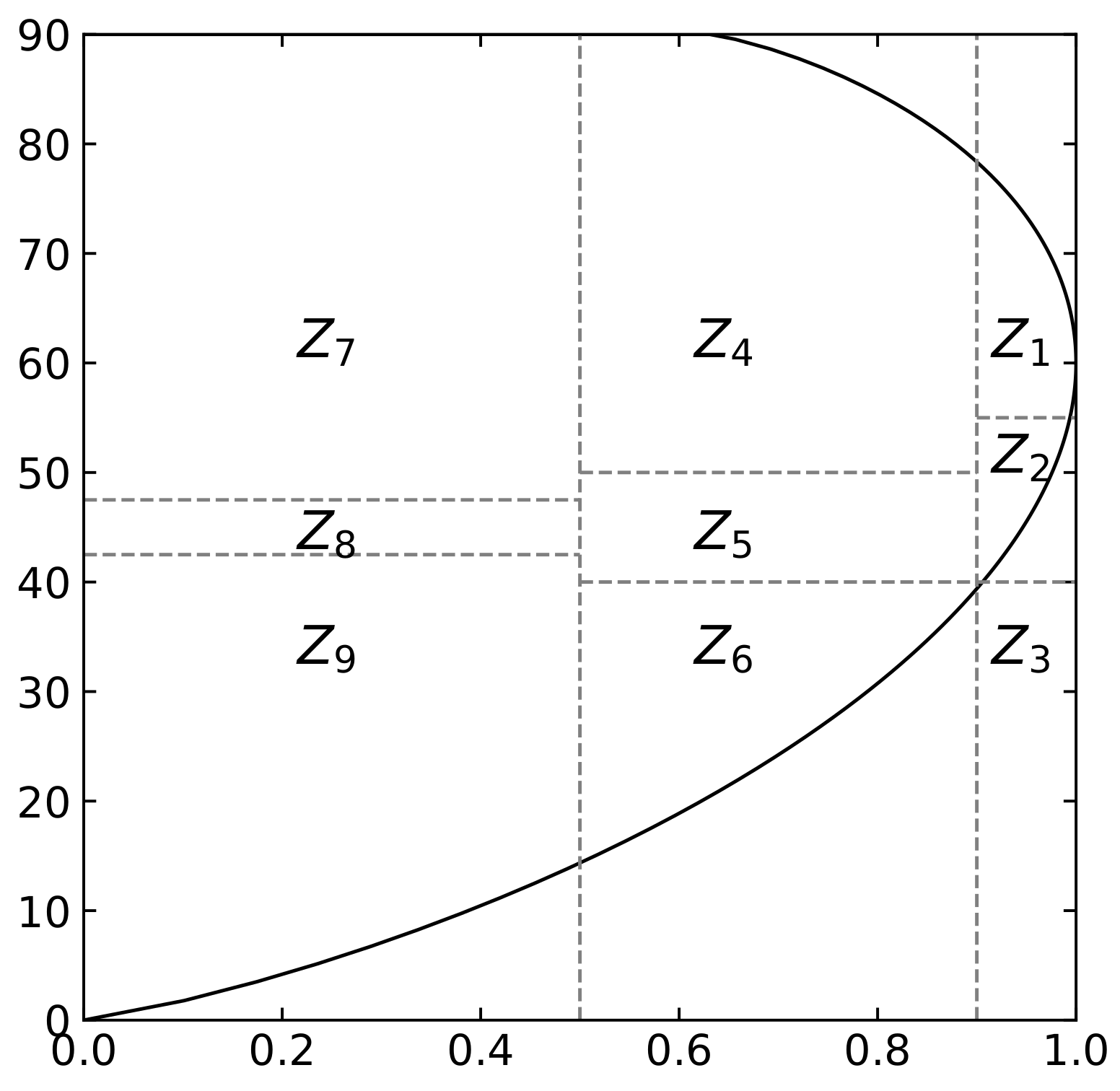
Cloude and Pottier [18] represented the random scattering mechanism in PolSAR images using two decomposition parameters—entropy and mean alpha angle—defined in (3) and obtained via eigenvalue decomposition of the polarimetric coherency matrix. Entropy describes the degree of randomness in scattering. For areas with a smooth surface such as water, surface scattering dominates, resulting in low randomness. For man-made areas, the scattering mechanisms are mixed, leading to medium entropy. In vegetation areas, multiple scattering mechanisms result in high scattering randomness. The value of the mean alpha angle ranges from 0 to 90 degrees, representing the continuous change of the main scattering mechanism of the land cover from surface scattering to double-bounce scattering and reaching a medium value in areas described as volume scattering. Pottier introduced anisotropy A to characterize the importance of two nondominant scattering mechanisms, which can be used as a supplement to distinguish the scattering characteristics of different land cover types when the value of entropy is high [33]. As depicted in Figure 3, the results of Cloude–Pottier decomposition enable the rough identification of the three basic land cover types in the area: water, man-made, and vegetation. By combining entropy and the mean alpha angle, the classification hyperplane was proposed [18], as shown in Figure 4.
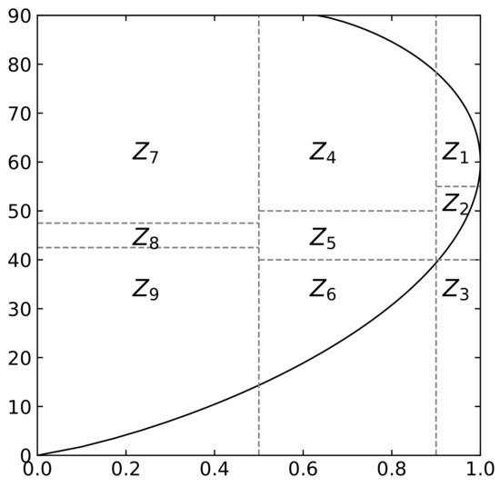
Figure 4.
classification hyperplane.
The polarimetric scattering characteristics are partitioned into nine regions, to , by a two-dimensional classification hyperplane based on predetermined thresholds for entropy and alpha angle. As the scattering characteristics of the surface cannot be discerned when , the high entropy surface scattering region is not an effective region on the classification hyperplane. To further enhance this approach, a classification scheme that incorporates anisotropy has been proposed [33], and the classification hyperplanes and results are presented in Figure 5.

Figure 5.
Classification hyperplanes and results of of the RadarSat-2 PolSAR image. (a) Result of hyperplane. (b) Result of hyperplane. (c) Result of hyperplane.
The method can be used to obtain the classification results of fundamental land cover types. Furthermore, more precise types can be achieved by employing other decomposition methods [9,10]. These methods not only allow for the identification of most land cover types in PolSAR images, but also offer a considerable degree of flexibility and generality. This is because the classification boundaries are determined based on the extracted physical information from the microwave scattering observations. Therefore, the pseudo-labels constructed using these methods are insensitive to data changes and independent of the data source. It should be noted that the selection and configuration of unsupervised classification methods are highly adaptable. Various target decomposition methods [8], hyperplane combinations [59], and threshold settings [60] can be utilized to construct pseudo-labels with the guidance of polarimetric scattering characteristics.
Up to this point, the construction of pseudo-labels has been accomplished. In order to further enhance the accuracy, we take inspiration from some existing studies [61,62,63] and compute the average value of the polarimetric coherency matrix for the pixels in each category obtained from the initial stage results. These average values are then employed as clustering centers for the Wishart distance-based classifier, which is used to reclassify all pixels. This process is iterated until the algorithm converges. The purpose of this approach is to refine and adjust the classification boundaries that were previously established by means of thresholds, thereby avoiding the occurrence of ambiguous classification results. Specifically, the center of the mth category can be obtained by calculating the sample mean:
where represents the total number of pixels contained in this category, and is the polarimetric coherency matrix of the ith pixel in the mth category. The distance measurement of classification is defined as follows:
where represents the trace operation of matrix. Based on the distance value from each center, each sample should be assigned to the category of the nearest cluster center. When a sample is assigned to the ith category, the following inequality holds:
Once all the sample points have been partitioned, the center of each category should be recalculated, and the above process should be repeated until convergence. This method is a fusion of polarimetric scattering characteristics and Wishart clustering. The former yields the initial classification results with category semantic information based on the distinct scattering mechanisms, while the latter takes into account the data distribution of the polarimetric coherency matrix. The combination not only preserves the category semantics in the unsupervised classification results, but also optimizes the classification boundaries to enhance the accuracy of the pseudo-labels. As a result of the aforementioned two steps, each pixel in the source and target images can be assigned a unique label . Therefore, the source dataset and the target dataset can be represented as and , respectively. Compared to pseudo-labels in related methods of optical image classification, the use of polarimetric scattering characteristics in PolSAR image classification can directly obtain pseudo-labels with a certain degree of accuracy. This eliminates the need for random initialization and the iterative refinement during the model training, making it significantly advantageous in terms of implementation difficulty and algorithmic complexity.
Utilization: Similar to previous works [31,32,56], we utilize class-wise alignment based on the obtained polarimetric scattering characteristics and constructed pseudo-labels. This is a straightforward approach to enhance the feature discriminability using the concept of metric learning, which functions to maximize interclass distance and minimize intraclass distance. Hence, we can formulate the following optimization problem:
where is a similarity measurement. The specific definition of can take many forms [64,65,66]. In the proposed PSCAN, we adopt a more direct approach, i.e., optimizing the cross-entropy loss:
where denotes the classifier for auxiliary task, which is designed to receive the category semantic information from polarimetric scattering characteristics-guided pseudo-labels. Equation (12) is also a good choice because it balances complexity and effectiveness. Compared with (11), the cross-entropy loss is undoubtedly more convenient, owing to its wide range of applications and ease of implementation. Additionally, it captures the interclass distance, which is the most important ability in improving feature discriminability.
Based on the above introduction, the objective function of PSCAN can be formulated as follows:
where is the trade-off hyperparameter. are optimization variables, but only are finally required. From (13), it is evident that the input data should initially be mapped into a latent space by the feature encoder f. Subsequently, the feature distributions of the source and target domains can be aligned with the precondition of ensuring discriminability by minimizing and . Finally, the classifier c can be learned from the source and generalized to the target.
The three items in (13) correspond to different objectives of the proposed PSCAN, which can be seen as an end-to-end multitask deep adaptation model. The following are specific analyses of these tasks:
The item corresponds to the task of predicting the manual annotations of source domain data, whose definition is same as the standard cross-entropy loss function, as shown in (5). Note that with the learning rate of the optimizer as , the parameter c corresponding to the classifier in the model will be updated as follows:
It is evident that the classifier training solely depends on the samples from the source domain. Therefore, the trained classifier, which can generalize well on the source domain based on the feature extractor f, forms the basis for generalization on the target domain during testing.
The term corresponds to the task of predicting the data source, as defined in (7). With the features extracted from the source and target data, the parameter d of the domain discriminator can be obtained by maximizing its prediction accuracy:
It can be observed from Equation (15) that the training of the domain discriminator does not require any manual annotations, as the data source serves as the supervisory information. The domain discriminator is employed to counteract the feature extractor, whereby it predicts the data source and minimizes the probability of prediction error. Meanwhile, the feature extractor aims to extract features that can deceive the domain discriminator; that is, it maximizes the probability of prediction error of the domain discriminator and aligns the feature distributions of the source and target domains. Therefore, the domain discriminator forms the foundation of extracting domain-invariant features.
The item corresponds to the task of predicting pseudo-labels, as defined in (12). The update of parameter in the auxiliary task can be expressed as follows:
The auxiliary task in PSCAN is designed to extract category semantic information from pseudo-labels using supervised learning. The pseudo-labels guide the auxiliary task to mine the category semantic information. Since the discriminability of source-specific feature extraction can be ensured by learning with manual annotations, and the true and pseudo-labels share the same category space, learning pseudo-labels of source and target domains can also lead to the discriminability of target features.
4. Experiments
4.1. Study Area and Data Sources
We have selected the Golden Gate Bridge area and its surrounding regions in San Francisco, CA, USA, as our research objects. This study area comprises both urban and suburban areas, making it ideal for evaluating the generalization performance of the proposed method. Our experiments involve PolSAR image data captured with three different sensors. These datasets were obtained from the Institute of Electronics and Telecommunications of Rennes (https://ietr-lab.univ-rennes1.fr/polsarpro-bio/san-francisco/ (accessed on 21 February 2023)), and the ground maps used for reference were labeled by the Intelligent Perception and Image Understanding Laboratory [67].
ALOS-2 San Francisco: This dataset was captured by the L-band satellite-bone PolSAR system ALOS-2 in March 2015. The spatial resolution is 18 m. The size of the image is . Figure 6a is the Pauli RGB map of this dataset, and Figure 6b shows the ground truth map.

Figure 6.
Pauli RGB and ground truth maps of the San Francisco datasets and the color code. (a,b) ALOS-2 San Francisco dataset. (c,d) GF-3 San Francisco dataset. (e,f) RS-2 San Francisco dataset.
GF-3 San Francisco: This dataset was captured by the C-band satellite-bone PolSAR system Gaofen 3 (GF-3) in September 2017. The spatial resolution is 8 m. The size of the image is . Figure 6c is the Pauli RGB map of this dataset, and Figure 6d shows the ground truth map.
RS-2 San Francisco: This dataset was captured by the C-band satellite-bone PolSAR system RadarSat-2 (RS-2) in April 2008. The spatial resolution is 8 m. The size of the image is . Figure 6e is the Pauli RGB map of this dataset, and Figure 6f shows the ground truth map.
In addition, we used PolSAR images from GF-3 and RS-2 near the Jiaozhou Bay cross-sea bridge in Qingdao, Shandong, China. The details are as follows.
GF-3 Qingdao: This dataset was captured with the GF-3 in November 2017. The spatial resolution is 4.73 m. The size of the image is . Figure 7a is the Pauli RGB map of this dataset, and Figure 7b shows the ground truth map.
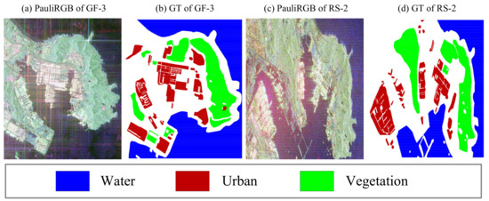
Figure 7.
Pauli RGB and ground truth maps of the Qingdao datasets and the color code. (a,b) GF-3 Qingdao dataset. (c,d) RS-2 Qingdao dataset.
4.2. Experimental Setup
Comparison methods: To validate the significance of the proposed method, both traditional learning methods and deep DA methods were chosen for comparison. Specifically, for traditional learning methods, we chose transfer component analysis (TCA) [50], joint distribution alignment (JDA) [68], balanced distribution adaptation (BDA) [69], and transfer joint matching (TJM) [70]. For deep DA methods, we chose deep adaptation network (DAN) [25], deep correlation alignment (DCORAL) [71], joint adaptation network (JAN) [27], domain adversarial neural network (DANN) [28], and conditional domain adversarial network (CDAN) [72].
Experiment settings: Before the training start, we prepared the pixel-centric PolSAR image patch with the size of for each dataset. Then the training and testing sets were obtained based on the ground truth maps in Figure 6. It needs to be pointed out that there is no overlap between the training and testing sets. When a dataset acts as the source domain, the label of its training set will be preserved; when it acts as the target domain, the label of the training set will be ignored. Therefore, six transfer tasks could be constructed based on the three datasets.
The prediction of the traditional learning methods is performed using the 1-nearest neighbor classifier based on feature alignment. The bandwidth of Gaussian kernels in multikernel MMD has a range of . To ensure fairness of comparison, the model parameters of all deep DA methods were shared. We used the Adam optimizer for the optimization of deep methods and iterated the training for 150 epochs with a batch size of 256. The learning rate was set to a small value of for the stability of the adversarial training, and the learning rate of the feature encoder was set to of that of the other parts for better convergence [73].
To evaluate the performance of involved adaptation methods, overall accuracy (OA), average accuracy (AA), and kappa coefficient (KC) were chosen as the evaluation criteria. The higher the values of OA, AA, and KC are, the better the model is.
4.3. Comparison of Results
Based on the above-mentioned settings, we conducted experiments on the existing transfer tasks to assess the effectiveness of the proposed method. The total experimental results are shown in Table 1, which contains the OA of the involved methods across all transfer tasks.

Table 1.
Comparison of the overall accuracy (%) on all transfer tasks. The A, G, and R in the first column represent the ALOS-2, GF-3, and RS-2 datasets, respectively, and the Avg means average of the performance of each task. With A→G taken as an example, the ALOS-2 is the source domain and GF-3 is the target domain. The best results are highlighted in bold.
The results demonstrate that the proposed PSCAN achieved the best performance in four out of six transfer tasks on the San Francisco area, with a suboptimal performance in one of the remaining two tasks. Therefore, as shown in the Avg column, the proposed method exhibited the highest overall accuracy across all transfer tasks. In comparison with traditional learning methods, there is a noticeable performance gap in the test results of deep DA methods, highlighting the significance of deep feature adaptation. Additionally, the performance of statistical criterion-based methods in deep DA is not as impressive as that of the adversarial loss-based ones, which is in line with current understanding. Moreover, the proposed PSCAN improves the overall accuracy by as compared to the second-best method DANN on the San Francisco area and by as compared to the second-best method CDAN on the Qingdao area. Considering that the models of both methods are identical, except for the incorporation of the auxiliary task in PSCAN, we can attribute the improvement in performance to the utilization of the polarimetric scattering characteristics. This observation substantiates the potential of the proposed method in achieving effective knowledge transfer, leading to satisfactory unsupervised classification results.
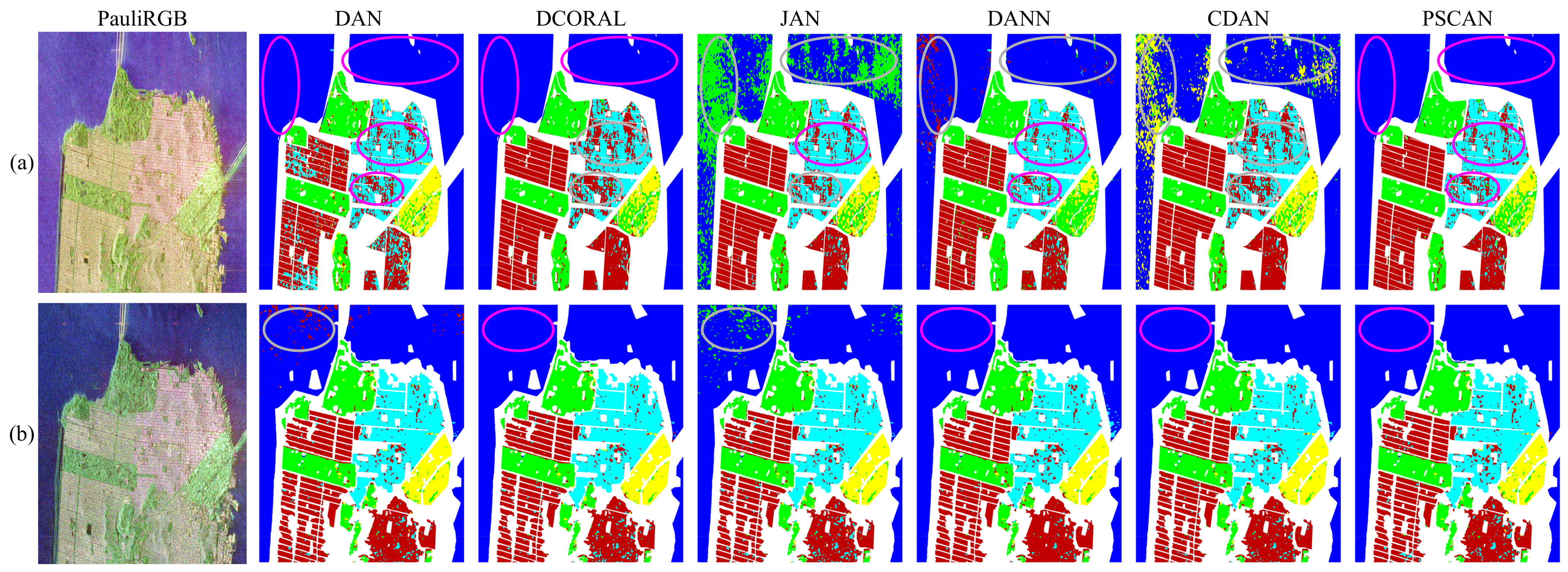
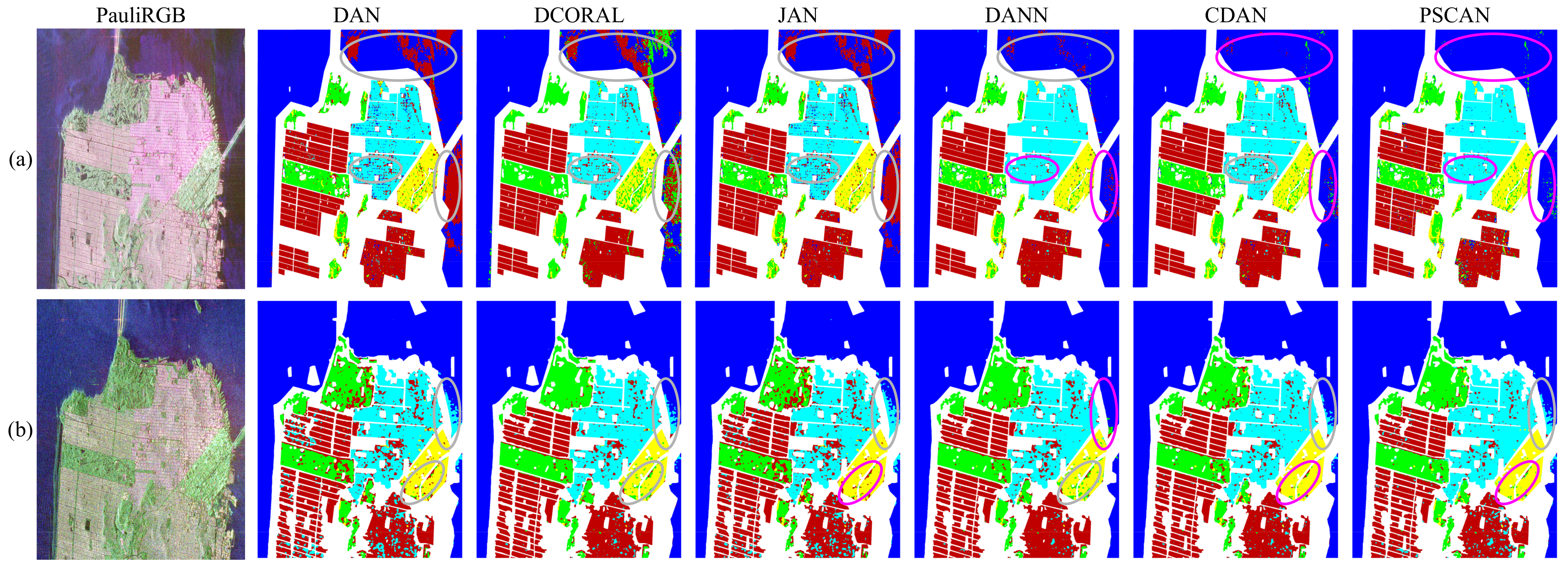
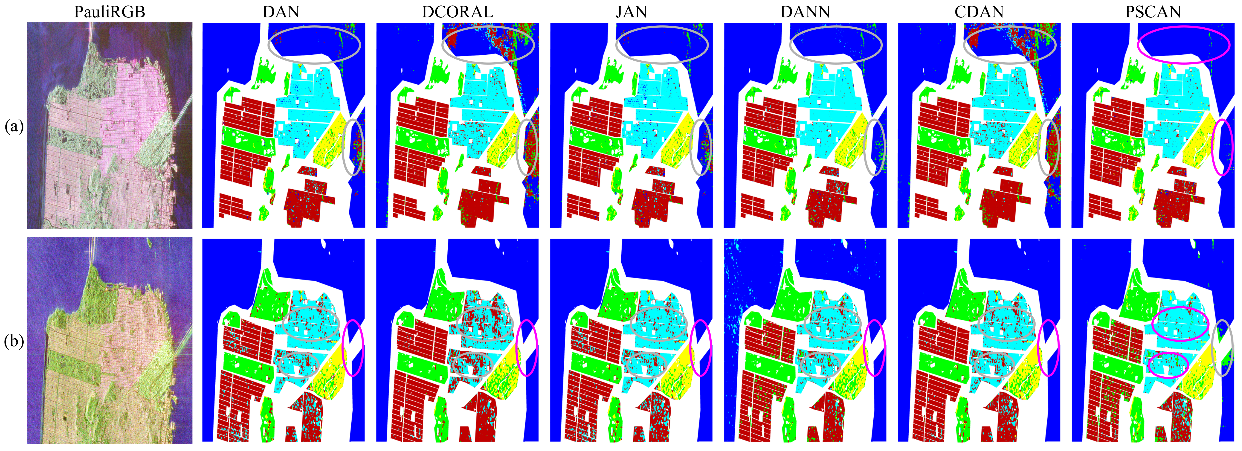
Table 2, Table 3, Table 4 and Table 5 present the performance of each method in the transfer task under a specific source domain, including the accuracy of each category, AA and KC. The corresponding whole map classification results can be seen from Figure 8, Figure 9, Figure 10 and Figure 11. Based on these results, we provide the following analysis.

Table 2.
Comparison of experimental results (%) on the San Francisco area when the source domain is set to ALOS-2. The C1 to C5 refer to different categories: Water, Vegetation, High-Density Urban, Low-Density Urban, and Developed.

Table 3.
Comparison of experimental results (%) on the San Francisco area when the source domain is set to GF-3.

Table 4.
Comparison of experimental results (%) on the San Francisco area when the source domain is set to RS-2.

Table 5.
Comparison of experimental results (%) on the Qingdao area. The C1 to C3 refer to different respective categories: Urban, Vegetation, and Water.
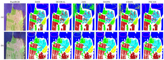
Figure 8.
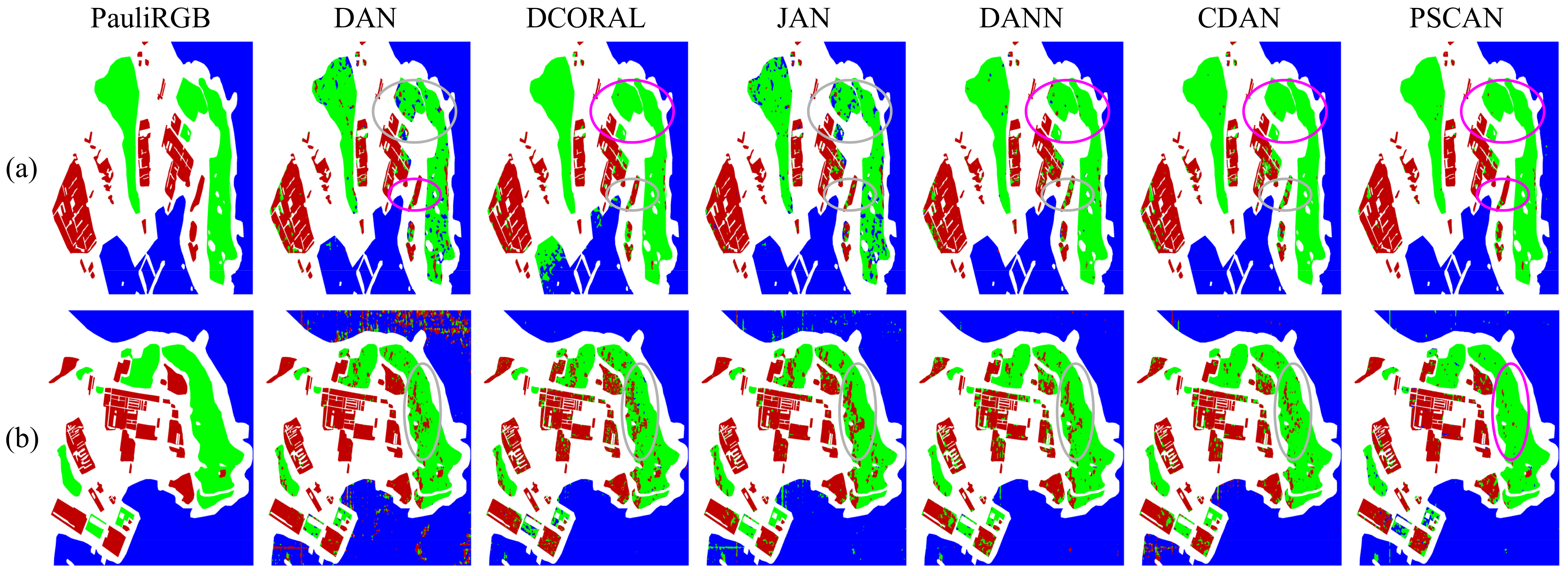
Comparison of the whole map classification results on the San Francisco area when the source domain is set to ALOS-2. The circles in pink and gray represent the correct and incorrect classification, respectively. (a) GF-3 as the target domain. (b) RS-2 as the target domain.
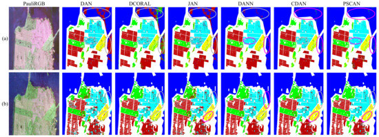
Figure 9.
Comparison of the whole map classification results on the San Francisco area when the source domain is set to GF-3. The circles in pink and gray represent the correct and incorrect classification, respectively. (a) ALOS-2 as the target domain. (b) RS-2 as the target domain.
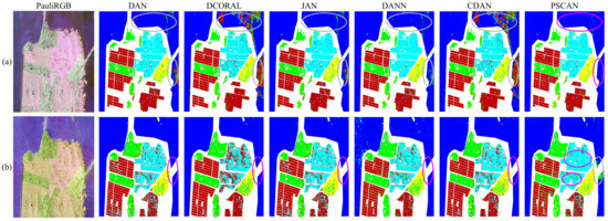
Figure 10.
Comparison of the whole map classification results on the San Francisco area when the source domain is set to RS-2. (a) ALOS-2 as the target domain. (b) GF-3 as the target domain.
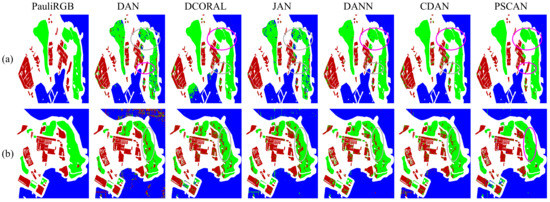
Figure 11.
Comparison of the whole map classification results on the Qingdao area. The circles in pink and gray represent the correct and incorrect classification, respectively. (a) RS-2 as the target domain. (b) GF-3 as the target domain.
In the case of the source domain being ALOS-2, we present a detailed comparison of the experimental results of the involved methods in Table 2, and the whole map classification results are illustrated in Figure 8. For the first task, i.e., ALOS-2→GF-3, the proposed PSCAN achieved the best testing results. As indicated in Table 2, the proposed method shows a certain degree of improvement compared to most of the compared methods. Specifically, the OA and KC are and higher, respectively, than is the suboptimal DAN method, and the whole map classification result of PSCAN is significantly closer to the ground truth map. For the task of ALOS-2→RS-2, all deep DA methods demonstrate good classification performance, and the variation between the proposed method and the model with the highest accuracy is approximately .
A comprehensive comparison of experimental results for the respective methods when the source domain is set to GF-3 is presented in Table 3, and the whole map classification results are illustrated in Figure 9. The highest level of accuracy during testing was attained by the proposed PSCAN when the target domain was assigned as RS-2. This same conclusion can be drawn from Figure 9, where PSCAN demonstrates superior classification results in the marked areas. For the other transfer task, PSCAN yields suboptimal testing results but it is only about behind the optimal result in both AA and KC. The addition of the auxiliary task improves the classification accuracy of the baseline for Vegetation and Low-Density Urban in the first task as well as Low-Density Urban and Developed in the second task.
A detailed comparison of experimental results for the involved methods when the source domain is set to RS-2 is presented in Table 4, while the whole map classification results are illustrated in Figure 10. PSCAN outperformed the previous two methods in this experimental setting, achieving the best results in both transfer tasks. Specifically, for the RS-2→GF-3 task, the proposed PSCAN achieved about a increase in both AA and KC metrics. The conclusions derived from the whole map classification results are consistent with those drawn from the testing results. As indicated in Figure 10a, the performance of PSCAN in the two marked regions is significantly better than other methods. Although Figure 10b shows that the classification performance of PSCAN for water is slightly inferior, it exhibits the best classification performance for urban areas. Moreover, the addition of the auxiliary task improves the accuracy for Low-Density Urban in the first task and Developed in the both tasks.
We present the detailed experimental results on the Qingdao area in Table 5, following a similar approach as that for the San Francisco area. The Qingdao area contains only two datasets, resulting in two transfer tasks: GF-3 as the source domain and RS-2 as the target domain, or RS-2 as the source domain and GF-3 as the target domain. Our results show that the classification performance of the method without adaptation is unsatisfactory and has the lowest classification accuracy among all methods, regardless of the source and target domains. However, when RS-2 is set as the target domain, the traditional UDA methods perform well, and both BDA and TJM methods have similar classification accuracy to the deep UDA methods. However, when GF-3 is used as the target domain, the performance of these methods decreases significantly, which reflects the limitations of using shallow features. In contrast, the performance of deep UDA methods remains relatively stable in both transfer tasks, and the performance of three ADA-based methods is higher. In comparison with other methods, the proposed method achieves the most outstanding classification performance. When RS-2 is the target domain, the proposed method’s evaluation criteria are , , and higher than those of the second-best DANN method. With GF-3 as the target domain, the proposed method’s evaluation criteria are also , , and higher than those of the second-best CDAN method, which clearly demonstrates its advantages. It achieves the optimal or suboptimal accuracy in the classification of Urban, Vegetation in both tasks. In summary, the proposed method results in an increase of about in OA and AA, and the performance improves by more than compared to that before adaptation.
Figure 11 shows the whole map classification results on the Qingdao area. Similar to the previous ones, the meanings of the results of each row and the circles are given in the caption. From the results, it can be seen that the proposed method achieves the best classification results on both tasks. The conclusions reflected in the classification maps are consistent with the quantitative results, which can verify the effectiveness of the proposed PSCAN.
4.4. Effect of Hyperparameter
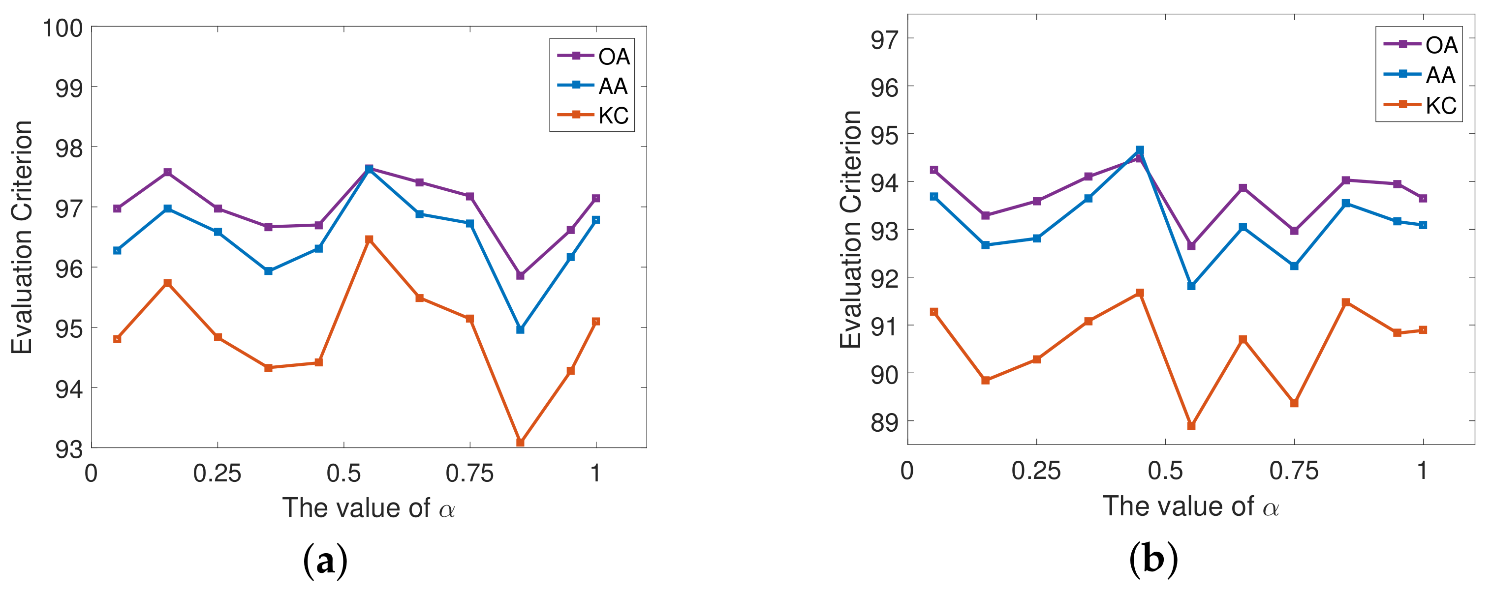
As shown in (13), the value of hyperparameter reflects how much the model pays attention to the auxiliary task in the process of adversarial training. Using the Qingdao datasets, we analyzed the influence of on the model performance. The experimental results are shown in Figure 12.
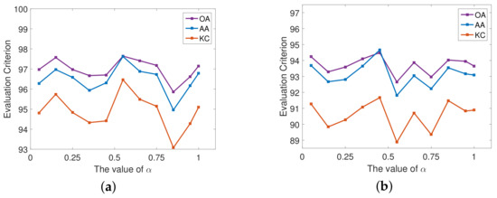
Figure 12.
Effect of on classification performance of the proposed PSCAN. (a) Results when RS-2 is the target. (b) Results when GF-3 is the target.
According to the experimental settings, we set the value of within . From the experimental results, it can be seen that when GF-3 is the source domain and RS-2 is the target domain, the classification performance is poor when the is around , and the OA changes slightly between and in the other times. When RS-2 is source and GF-3 is target, the performance of PSCAN is poor when the value of is between and , and the change of OA is relatively stable when using other values.
4.5. Feature Visualization Results
We used the San Francisco datasets, taking ALOS-2 as the source and GF-3 as the target to train the network. Then, principal component analysis (PCA) was used to reduce the dimension of features extracted before and after the adaption to realize the feature visualization so as to verify the effectiveness of the proposed method in improving the transferability and discriminability of features.
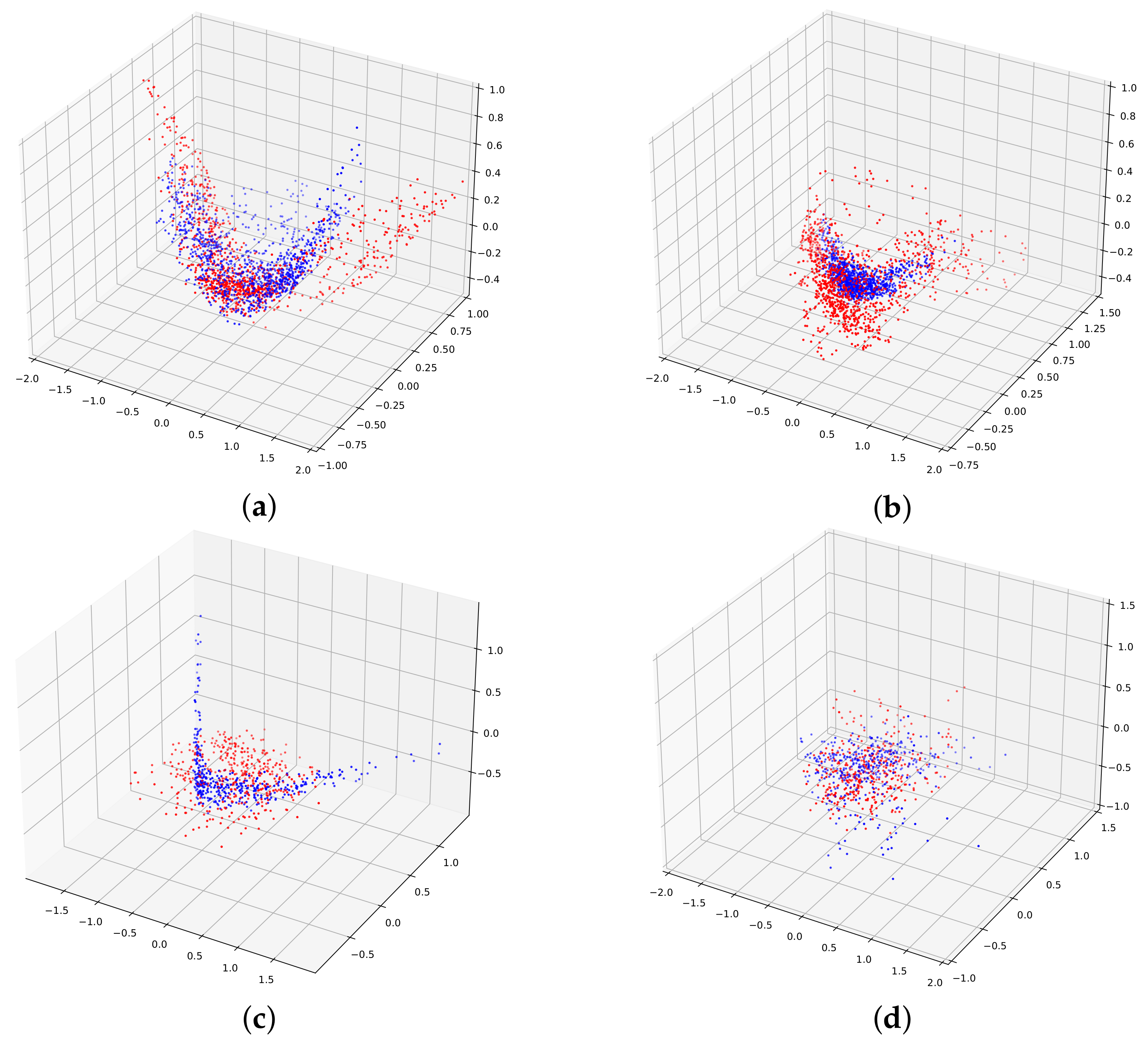
Feature distributions of the data under two categories of Water and Low-Density Urban with low classification accuracy are compared in Figure 13, where the red scatter represents the source data and the blue is the target data.

Figure 13.
Comparison of feature distributions between the source and target data before and after adaptation. (a) Feature distribution of Water data before adaptation. (b) Feature distribution of water data after adaptation. (c) Feature distribution of Low-Density Urban data before adaptation. (d) Feature distribution of low-density urban data after adaptation.
The experiment used the features corresponding to the first three principal components extracted by PCA to form a three-dimensional space. Compared with the feature visualization result after adaptation, the scatter points in the result before adaptation were more distant from each other, and their spatial distribution was more dispersed, which shows that the proposed method can effectively align the feature distribution of source and target domains, and extract features with transferability.
Then, we compared the feature distribution of all categories of target data before and after adaptation. By reducing the dimension of features extracted from the target domain to two and observing the distance between categories in the two-dimensional plane, the discriminability of the target domain features can be inferred.
As shown in Figure 14a, the samples of Water and Vegetation, High-Density Urban and Low-Density Urban, and Vegetation and Developed have a certain degree of overlap in spatial distribution. In contrast, the result shown in Figure 14b have better feature discriminability, which is reflected in the samples of the Water category being far away from the ones of other categories the fewer overlapping areas between High-Density Urban and Low-Density Urban and between Vegetation and Developed than the result before adaptation. These results prove the effectiveness of the proposed method in improving the discriminability of target features.
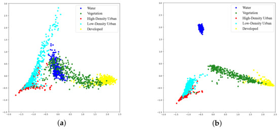
Figure 14.
Comparison of the feature discriminability of target data before and after adaptation. (a) Target feature visualization before adaptation. (b) Target feature visualization after adaptation.
4.6. Ablation Experiments
The auxiliary task for receiving the guidance from polarimetric scattering characteristics and the domain discriminator for aligning feature distributions are two important components as well as the keys to improvement. To verify their effectiveness, ablation experiments were conducted. It could be observed that the performance differences of DAN, DANN, and PSCAN can be used to verify this issue. When the hyperparameters of these models were set the same, the DAN could be seen as lacking the domain discriminator version of DANN, while the DANN could be seen as lacking the auxiliary task version of the proposed PSCAN.
Specific comparison results on the two areas are summarized in Figure 15, where the meaning of coordinate axis is consistent with that in Table 1. It can be seen that in the eight transfer tasks, the performance of the model with polarimetric scattering characteristics is better than or at least equal to that of the model without auxiliary task. In addition, the domain discriminator also plays a positive role in improving the accuracy in most cases. These observations show that the performance improvements should be attributed to the addition of the domain discriminator and our proposed auxiliary task, which ensure the transferability and discriminability of features, respectively. In addition, it also shows that the proposed method has the potential to improve the adaptive networks in a plug-and-play manner.
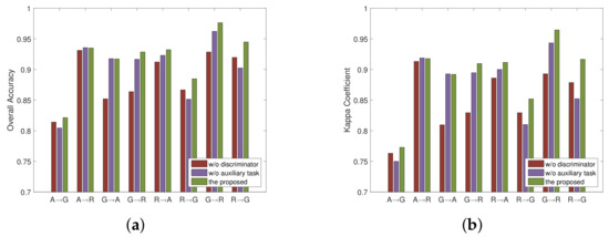
Figure 15.
Comparison results of the ablation study. (a) Results of OA. (b) Results of KC.
5. Conclusions
This paper presents a novel adversarial learning approach for the unsupervised classification of PolSAR images. Its innovation is reflected in the following aspects: First, the proposed method builds upon the unexplored deep unsupervised DA studies while taking into account the specific characteristics of PolSAR images. Second, given that PolSAR data contains unique information, we designed an auxiliary task to capture the polarimetric scattering characteristics and construct the pseudo-labels using a deep ADA model. This enables us to align the features of the source and target domains while ensuring both feature transferability and discriminability. Third, we propose a PSCAN method by explicitly modeling the feature confusion process. Experimental results demonstrate that our approach can extract domain-invariant and discriminative features and improve the performance on the target domain classification task.
Our experiments utilized datasets from three distinct PolSAR systems covering the San Francisco and Qingdao areas. The results demonstrate that our proposed method achieves superior unsupervised classification performance across most transfer tasks. Furthermore, we discuss the novelty, particularity, and applicable conditions of our approach.
While some progress has been achieved, shortcomings still exist, which are mainly reflected in the fact that the uncertainty in the process of pseudo-label construction has not received sufficient attention. In future work, we aim to address this issue through selective pseudo-labeling. Moreover, several unresolved issues in the PolSAR community, including improving the utilization of polarimetric information in the PolSAR data, exploring multisource-based adaptation techniques, and tackling domain generalization problems are all issues we are considering.
Author Contributions
All the authors made significant contributions to this work. H.D. and L.S. devised the approach and wrote the paper. H.D. and W.Q. conducted the experiments and analyzed the data. W.M., C.Z., Y.W. and L.Z. provided oversight and suggestions; W.Q. and W.M. performed the writing—review and editing. All authors have read and agreed to the published version of the manuscript.
Funding
This work was supported by National Nature Science Foundation of China (grant No. 62271172). The authors thank the IETR for providing the PolSAR data. The authors would also like to thank Xu Liu from the IPIU Laboratory, Xidian University, for discussions on data annotations.
Conflicts of Interest
The authors declare no conflict of interest.
References
- Mott, H. Remote Sensing with Polarimetric Radar; Wiley-IEEE Press: Hoboken, NJ, USA, 2007. [Google Scholar]
- Zhang, C.; Sargent, I.; Pan, X.; Li, H.; Gardiner, A.; Hare, J.; Atkinson, P.M. Joint Deep Learning for land cover and land use classification. Remote Sens. Environ. 2019, 221, 173–187. [Google Scholar] [CrossRef]
- Shi, H.; Zhao, L.; Yang, J.; Lopez-Sanchez, J.M.; Zhao, J.; Sun, W.; Shi, L.; Li, P. Soil moisture retrieval over agricultural fields from L-band multi-incidence and multitemporal PolSAR observations using polarimetric decomposition techniques. Remote Sens. Environ. 2021, 261, 112485. [Google Scholar] [CrossRef]
- Ma, X.; Xu, J.; Wu, P.; Kong, P. Oil Spill Detection Based on Deep Convolutional Neural Networks Using Polarimetric Scattering Information From Sentinel-1 SAR Images. IEEE Trans. Geosci. Remote Sens. 2022, 60, 4204713. [Google Scholar] [CrossRef]
- Zhang, T.; Quan, S.; Yang, Z.; Guo, W.; Zhang, Z.; Gan, H. A Two-Stage Method for Ship Detection Using PolSAR Image. IEEE Trans. Geosci. Remote Sens. 2022, 60, 5236918. [Google Scholar] [CrossRef]
- Moghaddam, M.; Saatchi, S. Analysis of scattering mechanisms in SAR imagery over boreal forest: Results from BOREAS’93. IEEE Trans. Geosci. Remote Sens. 1995, 33, 1290–1296. [Google Scholar] [CrossRef]
- Cloude, S.R.; Pottier, E. A review of target decomposition theorems in radar polarimetry. IEEE Trans. Geosci. Remote Sens. 1996, 34, 498–518. [Google Scholar] [CrossRef]
- Cameron, W.; Leung, L. Feature Motivated Polarization Scattering Matrix Decomposition. In Proceedings of the IEEE International Conference on Radar, Arlington, VA, USA, 7–10 May 1990; pp. 549–557. [Google Scholar] [CrossRef]
- Freeman, A.; Durden, S.L. A three-component scattering model for polarimetric SAR data. IEEE Trans. Geosci. Remote Sens. 1998, 36, 963–973. [Google Scholar] [CrossRef]
- Yamaguchi, Y.; Sato, A.; Boerner, W.; Sato, R.; Yamada, H. Four-component scattering power decomposition with rotation of coherency matrix. IEEE Trans. Geosci. Remote Sens. 2011, 49, 2251–2258. [Google Scholar] [CrossRef]
- Hara, Y.; Atkins, R.G.; Yueh, S.H.; Shin, R.T.; Kong, J.A. Application of neural networks to radar image classification. IEEE Trans. Geosci. Remote Sens. 1994, 32, 100–109. [Google Scholar] [CrossRef]
- Lee, J.S.; Grunes, M.R.; Kwok, R. Classification of multi-look polarimetric SAR imagery based on complex Wishart distribution. Int. J. Remote Sens. 1994, 15, 2299–2311. [Google Scholar] [CrossRef]
- Lardeux, C.; Frison, P.; Tison, C.; Souyris, J.; Stoll, B.; Fruneau, B.; Rudant, J. Support vector machine for multifrequency SAR polarimetric data classification. IEEE Trans. Geosci. Remote Sens. 2009, 47, 4143–4152. [Google Scholar] [CrossRef]
- Du, L.J.; Lee, J.S. Fuzzy classification of earth terrain covers using complex polarimetric SAR data. Int. J. Remote Sens. 1996, 17, 809–826. [Google Scholar] [CrossRef]
- Cao, F.; Hong, W.; Wu, Y.; Pottier, E. An Unsupervised Segmentation With an Adaptive Number of Clusters Using the SPAN/H/α/A Space and the Complex Wishart Clustering for Fully Polarimetric SAR Data Analysis. IEEE Trans. Geosci. Remote Sens. 2007, 45, 3454–3467. [Google Scholar] [CrossRef]
- Ersahin, K.; Cumming, I.G.; Ward, R.K. Segmentation and Classification of Polarimetric SAR Data Using Spectral Graph Partitioning. IEEE Trans. Geosci. Remote Sens. 2010, 48, 164–174. [Google Scholar] [CrossRef]
- van Zyl, J.J. Unsupervised classification of scattering behavior using radar polarimetry data. IEEE Trans. Geosci. Remote Sens. 1989, 27, 36–45. [Google Scholar] [CrossRef]
- Cloude, S.R.; Pottier, E. An entropy based classification scheme for land applications of polarimetric SAR. IEEE Trans. Geosci. Remote Sens. 1997, 35, 68–78. [Google Scholar] [CrossRef]
- Zhou, Y.; Wang, H.; Xu, F.; Jin, Y. Polarimetric SAR Image Classification Using Deep Convolutional Neural Networks. IEEE Geosci. Remote Sens. Lett. 2016, 13, 1935–1939. [Google Scholar] [CrossRef]
- Zhang, L.; Zhang, S.; Zou, B.; Dong, H. Unsupervised Deep Representation Learning and Few-Shot Classification of PolSAR Images. IEEE Trans. Geosci. Remote Sens. 2022, 60, 1–16. [Google Scholar] [CrossRef]
- Ren, B.; Zhao, Y.; Hou, B.; Chanussot, J.; Jiao, L. A Mutual Information-Based Self-Supervised Learning Model for PolSAR Land Cover Classification. IEEE Trans. Geosci. Remote Sens. 2021, 59, 9224–9237. [Google Scholar] [CrossRef]
- Wang, M.; Deng, W. Deep visual domain adaptation: A survey. Neurocomputing 2018, 312, 135–153. [Google Scholar] [CrossRef]
- Pan, S.J.; Yang, Q. A Survey on Transfer Learning. IEEE Trans. Knowl. Data Eng. 2010, 22, 1345–1359. [Google Scholar] [CrossRef]
- Garrett, W.; Diana, J.C. A Survey of Unsupervised Deep Domain Adaptation. arXiv 2020, arXiv:1812.02849. [Google Scholar]
- Long, M.; Cao, Y.; Wang, J.; Jordan, M.I. Learning Transferable Features with Deep Adaptation Networks. In Proceedings of the International Conference on Machine Learning, Lille, France, 6–11 July 2015; pp. 97–105. [Google Scholar]
- Sun, B.; Feng, J.; Saenko, K. Return of Frustratingly Easy Domain Adaptation. In Proceedings of the AAAI Conference on Artificial Intelligence, Phoenix, AZ, USA, 12–17 February 2016; pp. 2058–2065. [Google Scholar]
- Long, M.; Zhu, H.; Wang, J.; Jordan, M.I. Deep Transfer Learning with Joint Adaptation Networks. In Proceedings of the ICML’17: Proceedings of the 34th International Conference on Machine Learning, Sydney, Australia, 6–11 August 2017; pp. 2208–2217. [Google Scholar]
- Ganin, Y.; Ustinova, E.; Ajakan, H.; Germain, P.; Larochelle, H.; Laviolette, F.; Marchand, M.; Lempitsky, V. Domain-adversarial training of neural networks. J. Mach. Learn. Res. 2016, 17, 2030–2096. [Google Scholar]
- Tzeng, E.; Hoffman, J.; Saenko, K.; Darrell, T. Adversarial Discriminative Domain Adaptation. In Proceedings of the 2017 IEEE Conference on Computer Vision and Pattern Recognition (CVPR), Honolulu, HI, USA, 21–26 July 2017; pp. 7167–7176. [Google Scholar]
- Chen, X.; Wang, S.; Long, M.; Wang, J. Transferability vs. Discriminability: Batch Spectral Penalization for Adversarial Domain Adaptation. In Proceedings of the 36th International Conference on Machine Learning, Long Beach, CA, USA, 9–15 June 2019; pp. 1081–1090. [Google Scholar]
- Kang, G.; Jiang, L.; Yang, Y.; Hauptmann, A.G. Contrastive Adaptation Network for Unsupervised Domain Adaptation. In Proceedings of the IEEE/CVF Conference on Computer Vision and Pattern Recognition (CVPR), Long Beach, CA, USA, 15–20 June 2019; pp. 4888–4897. [Google Scholar] [CrossRef]
- Pei, Z.; Cao, Z.; Long, M.; Wang, J. Multi-Adversarial Domain Adaptation. In Proceedings of the AAAI Conference on Artificial Intelligence, New Orleans, LO, USA, 2–7 February 2018; pp. 3934–3941. [Google Scholar]
- Pottier, E. The H/A/α Polarimetric Decomposition Approach Applied to PolSAR Data Processing. In Proceedings of the PIERS—Workshop on Advances in Radar Methods, Baveno, Italy, 20–22 July 1998; pp. 120–122. [Google Scholar]
- LeCun, Y.; Boser, B.; Denker, J.; Henderson, D.; Howard, R.; Hubbard, W.; Jackel, L. Backpropagation Applied to Handwritten Zip Code Recognition. Neural Comput. 1989, 1, 541–551. [Google Scholar] [CrossRef]
- Krizhevsky, A.; Sutskever, I.; Hinton, G.E. ImageNet Classification with Deep Convolutional Neural Networks. In Proceedings of the Advances in Neural Information Processing Systems 25 (NIPS 2012), Lake Tahoe, NV, USA, 3–6 December 2012; pp. 1097–1105. [Google Scholar] [CrossRef]
- Lecun, Y.; Bengio, Y.; Hinton, G.E. Deep learning. Nature 2015, 521, 436–444. [Google Scholar] [CrossRef]
- Chen, S.; Tao, C. PolSAR Image Classification Using Polarimetric-Feature-Driven Deep Convolutional Neural Network. IEEE Geosci. Remote Sens. Lett. 2018, 15, 627–631. [Google Scholar] [CrossRef]
- Liu, X.; Jiao, L.; Tang, X.; Sun, Q.; Zhang, D. Polarimetric Convolutional Network for PolSAR Image Classification. IEEE Trans. Geosci. Remote Sens. 2019, 57, 3040–3054. [Google Scholar] [CrossRef]
- Zhang, L.; Dong, H.; Zou, B. Efficiently utilizing complex-valued PolSAR image data via a multi-task deep learning framework. ISPRS J. Photogramm. Remote Sens. 2019, 157, 59–72. [Google Scholar] [CrossRef]
- Zhang, Z.; Wang, H.; Xu, F.; Jin, Y. Complex-valued Convolutional Neural Network and Its Application in Polarimetric SAR Image Classification. IEEE Trans. Geosci. Remote Sens. 2017, 55, 7177–7188. [Google Scholar] [CrossRef]
- Yang, C.; Hou, B.; Ren, B.; Hu, Y.; Jiao, L. CNN-Based Polarimetric Decomposition Feature Selection for PolSAR Image Classification. IEEE Trans. Geosci. Remote Sens. 2019, 57, 8796–8812. [Google Scholar] [CrossRef]
- Qin, R.; Fu, X.; Lang, P. PolSAR Image Classification Based on Low-Frequency and Contour Subbands-Driven Polarimetric SENet. IEEE J. Sel. Topics Appl. Earth Observ. Remote Sens. 2020, 13, 4760–4773. [Google Scholar] [CrossRef]
- Dong, H.; Zhang, L.; Lu, D.; Zou, B. Attention-Based Polarimetric Feature Selection Convolutional Network for PolSAR Image Classification. IEEE Geosci. Remote Sens. Lett. 2020, 19, 4001705. [Google Scholar] [CrossRef]
- Dong, H.; Zhang, L.; Zou, B. PolSAR Image Classification with Lightweight 3D Convolutional Networks. Remote Sens. 2020, 12, 396. [Google Scholar] [CrossRef]
- Tan, X.; Li, M.; Zhang, P.; Wu, Y.; Song, W. Complex-Valued 3-D Convolutional Neural Network for PolSAR Image Classification. IEEE Geosci. Remote Sens. Lett. 2020, 17, 1022–1026. [Google Scholar] [CrossRef]
- Dong, H.; Zou, B.; Zhang, L.; Zhang, S. Automatic Design of CNNs via Differentiable Neural Architecture Search for PolSAR Image Classification. IEEE Trans. Geosci. Remote Sens. 2020, 58, 6362–6375. [Google Scholar] [CrossRef]
- Liu, F.; Jiao, L.; Tang, X. Task-Oriented GAN for PolSAR Image Classification and Clustering. IEEE Trans. Neural Netw. Learn. Syst. 2019, 30, 2707–2719. [Google Scholar] [CrossRef] [PubMed]
- Wen, Z.; Wu, Q.; Liu, Z.; Pan, Q. Polar-Spatial Feature Fusion Learning With Variational Generative-Discriminative Network for PolSAR Classification. IEEE Trans. Geosci. Remote Sens. 2019, 57, 8914–8927. [Google Scholar] [CrossRef]
- Zhu, X.; Montazeri, S.; Ali, M.; Hua, Y.; Wang, Y.; Mou, L.; Shi, Y.; Xu, F.; Bamler, R. Deep Learning Meets SAR: Concepts, Models, Pitfalls, and Perspectives. IEEE Geosci. Remote Sens. Mag. 2021, 9, 143–172. [Google Scholar] [CrossRef]
- Pan, S.J.; Tsang, I.W.; Kwok, J.T.; Yang, Q. Domain Adaptation via Transfer Component Analysis. IEEE Trans. Neural Netw. 2011, 22, 199–210. [Google Scholar] [CrossRef]
- Baktashmotlagh, M.; Harandi, M.T.; Lovell, B.C.; Salzmann, M. Unsupervised Domain Adaptation by Domain Invariant Projection. In Proceedings of the 2013 IEEE International Conference on Computer Vision, Sydney, NSW, Australia, 1–8 December 2013; pp. 769–776. [Google Scholar] [CrossRef]
- Zhuang, F.; Cheng, X.; Luo, P.; Pan, S.J.; He, Q. Supervised Representation Learning: Transfer Learning with Deep Autoencoders. In Proceedings of the IJCAI’15: 24th International Conference on Artificial Intelligence, Buenos Aires, Argentina, 25–31 July 2015; pp. 4119–4125. [Google Scholar]
- Goodfellow, I.; Pouget-Abadie, J.; Mirza, M.; Xu, B.; Warde-Farley, D.; Ozair, S.; Courville, A.; Bengio, Y. Generative Adversarial Nets. In Proceedings of the Advances in Neural Information Processing Systems 27 (NIPS 2014), Montreal, QC, Canada, 8–13 December 2014; pp. 2672–2680. [Google Scholar]
- Ioffe, S.; Szegedy, C. Batch Normalization: Accelerating Deep Network Training by Reducing Internal Covariate Shift. In Proceedings of the ICML’15: 32nd International Conference on International Conference on Machine Learning, Lille, France, 7–9 July 2015; pp. 448–456. [Google Scholar]
- Qiang, W.; Li, J.; Zheng, C.; Su, B. Auxiliary task guided mean and covariance alignment network for adversarial domain adaptation. Knowl.-Based Syst. 2021, 223, 107066. [Google Scholar] [CrossRef]
- Hou, C.; Tsai, Y.H.; Yeh, Y.R.; Wang, Y.F. Unsupervised Domain Adaptation With Label and Structural Consistency. IEEE Trans. Image Process. 2016, 25, 5552–5562. [Google Scholar] [CrossRef]
- Liang, J.; He, R.; Sun, Z.; Tan, T. Exploring uncertainty in pseudo-label guided unsupervised domain adaptation. Pattern Recognit. 2019, 96, 106996. [Google Scholar] [CrossRef]
- Wang, Q.; Breckon, T. Unsupervised Domain Adaptation via Structured Prediction Based Selective Pseudo-Labeling. In Proceedings of the AAAI Conference on Artificial Intelligence, New York, NY, USA, 7–12 February 2020; pp. 6243–6250. [Google Scholar]
- Yin, J.; Moon, W.M.; Yang, J. Novel Model-Based Method for Identification of Scattering Mechanisms in Polarimetric SAR Data. IEEE Trans. Geosci. Remote Sens. 2016, 54, 520–532. [Google Scholar] [CrossRef]
- Lu, D.; Zou, B. Improved alpha angle estimation of polarimetric SAR data. Electron. Lett. 2016, 52, 393–395. [Google Scholar] [CrossRef]
- Lee, J.S.; Grunes, M.R.; Ainsworth, T.; Du, L.J.; Schuler, D.L.; Cloude, S.R. Unsupervised classification using polarimetric decomposition and the complex Wishart classifier. IEEE Trans. Geosci. Remote Sens. 1999, 37, 2249–2258. [Google Scholar] [CrossRef]
- Ferro-Famil, L.; Pottier, E.; Lee, J.S. Unsupervised classification of multifrequency and fully polarimetric SAR images based on the H/A/Alpha-Wishart classifier. IEEE Trans. Geosci. Remote Sens. 2001, 39, 2332–2342. [Google Scholar] [CrossRef]
- Lee, J.S.; Grunes, M.R.; Pottier, E.; Ferro-Famil, L. Unsupervised terrain classification preserving polarimetric scattering characteristics. IEEE Trans. Geosci. Remote Sens. 2004, 42, 722–731. [Google Scholar] [CrossRef]
- Wen, Y.; Zhang, K.; Li, Z.; Qiao, Y. A Discriminative Feature Learning Approach for Deep Face Recognition. In Proceedings of the Computer Vision ECCV 2016: 14th European Conference, Amsterdam, The Netherlands, 11–14 October 2016; pp. 499–515. [Google Scholar]
- Schroff, F.; Kalenichenko, D.; Philbin, J. FaceNet: A Unified Embedding for Face Recognition and Clustering. In Proceedings of the IEEE Conference on Computer Vision and Pattern Recognition, Boston, MA, USA, 7–12 June 2015; pp. 815–823. [Google Scholar] [CrossRef]
- Liu, W.; Wen, Y.; Yu, Z.; Yang, M. Large-Margin Softmax Loss for Convolutional Neural Networks. In Proceedings of the ICML’16: 33rd International Conference on International Conference on Machine Learning, New York, NY, USA, 19–24 June 2016; pp. 507–516. [Google Scholar]
- Liu, X.; Jiao, L.; Liu, F. PolSF: PolSAR image dataset on San Francisco. arXiv 2019, arXiv:1912.07259. [Google Scholar]
- Long, M.; Wang, J.; Ding, G.; Sun, J.; Yu, P.S. Transfer Feature Learning with Joint Distribution Adaptation. In Proceedings of the 2013 IEEE International Conference on Computer Vision, Sydney, NSW, Australia, 1–8 December 2013; pp. 2200–2207. [Google Scholar] [CrossRef]
- Wang, J.; Chen, Y.; Hao, S.; Feng, W.; Shen, Z. Balanced Distribution Adaptation for Transfer Learning. In Proceedings of the 2017 IEEE International Conference on Data Mining (ICDM), New Orleans, LA, USA, 18–21 November 2017; pp. 1129–1134. [Google Scholar] [CrossRef]
- Long, M.; Wang, J.; Ding, G.; Sun, J.; Yu, P.S. Transfer Joint Matching for Unsupervised Domain Adaptation. In Proceedings of the 2014 IEEE Conference on Computer Vision and Pattern Recognition, Columbus, OH, USA, 23–28 June 2014; pp. 1410–1417. [Google Scholar] [CrossRef]
- Sun, B.; Saenko, K. Deep coral: Correlation alignment for deep domain adaptation. In Proceedings of the Computer Vision—ECCV 2016 Workshops, Amsterdam, The Netherlands, 8–10, 15–16 October 2016; pp. 443–450. [Google Scholar]
- Long, M.; Cao, Z.; Wang, J.; Jordan, M.I. Conditional Adversarial Domain Adaptation. In Proceedings of the Advances in Neural Information Processing Systems 31: Annual Conference on Neural Information Processing Systems, NeurIPS, Montréal, QC, Canada, 3–8 December 2018; pp. 1640–1650. [Google Scholar]
- Heusel, M.; Ramsauer, H.; Unterthiner, T.; Nessler, B.; Hochreiter, S. GANs Trained by a Two Time-Scale Update Rule Converge to a Local Nash Equilibrium. In Proceedings of the NIPS’17: 31st International Conference on Neural Information Processing Systems, Long Beach, CA, USA, 4–9 December 2017; pp. 6626–6638. [Google Scholar]
Disclaimer/Publisher’s Note: The statements, opinions and data contained in all publications are solely those of the individual author(s) and contributor(s) and not of MDPI and/or the editor(s). MDPI and/or the editor(s) disclaim responsibility for any injury to people or property resulting from any ideas, methods, instructions or products referred to in the content. |
© 2023 by the authors. Licensee MDPI, Basel, Switzerland. This article is an open access article distributed under the terms and conditions of the Creative Commons Attribution (CC BY) license (https://creativecommons.org/licenses/by/4.0/).


