Abstract
Radar emitter identification (REI) aims to extract the fingerprint of an emitter and determine the individual to which it belongs. Although many methods have used deep neural networks (DNNs) for an end-to-end REI, most of them only focus on a single view of signals, such as spectrogram, bi-spectrum, signal waveforms, and so on. When the electromagnetic environment varies, the performance of DNN will be significantly degraded. In this paper, a multi-view adaptive fusion network (MAFN) is proposed by simultaneously exploring the signal waveform and ambiguity function (AF). First, the original waveform and ambiguity function of the radar signals are used separately for feature extraction. Then, a multi-scale feature-level fusion module is constructed for the fusion of multi-view features from waveforms and AF, via the Atrous Spatial Pyramid Pooling (ASPP) structure. Next, the class probability is modeled as Dirichlet distribution to perform adaptive decision-level fusion via evidence theory. Extensive experiments are conducted on two datasets, and the results show that the proposed MAFN can achieve accurate classification of radar emitters and is more robust than its counterparts.
1. Introduction
Radar emitter identification (REI) is a key technology in radar signal processing, which aims to extract features of radar emitters to identify radar attributes and types. As a typical pattern recognition problem, REI can provide intelligence for reconnaissance and operational decisions in electronic countermeasures. In the early years, the signal waveform of a radar emitter is simple and the modulation parameters are stable, so the template matching method is usually used for REI [1]. First, a parameter feature template of each radar emitter, such as the pulse descriptor word (PDW), is established in advance. Then, the radar parameters are compared with those of the templates, to perform a pattern matching to identify the radar emitter. However, with the rapid development of radar systems and the increasing complexity of the electromagnetic environment, simple parameter matching cannot correctly identify radar emitters.
REI can be mainly divided into feature extraction and classification, and recently much effort has been made to design stable, finer and discriminative features, and reliable classifiers. For example, Kawalec et al. [2] extract the rise/fall time, rise/fall angle, rise and fall intersection point, top fall time, envelope UFMOP curve, and its regression line as emitter features, followed by linear discriminant analysis (LDA), for REI. Ru et al. [3] consider the rising edge of the envelope and part of the pulse peak as emitter features. Zhao et al. [4] estimate the instantaneous frequency of the signals and take the geometric features of the frequency drift curve as emitter features. In [5], Cao et al. compute the bi-spectrum amplitude spectrum of the signal and use an extreme learning machine (ELM) to automatically learn the signal features. To reduce the computational complexity of REI, Chen et al. [6] take the amplitude and phase of the first quadrant of the bi-spectrum as features for REI. In [7], a one-dimensional circular spectrum slice with a spectral frequency of zero is taken as the emitter feature. In [8], Wang first uses short-time Fourier transformation (STFT) of signals for REI and then uses random projection and principal component analysis (PCA) to extract features. In [9], Seddighi performs stripe or block segmentation of the Choi–William distribution (CWD) of radar signals, along the time axis, frequency axis, and time–frequency plane, respectively. The entropy, kurtosis, and skewness of each block are extracted as the emitter features. Also, the components of variational mode decomposition (VMD) are used as the emitter features in [10]. Based on the extracted emitter features, various types of classifiers are also developed for REI [11], including vector neural network (VNN) [12], support vector machine (SVM) [13], and so on.
In recent years, deep neural networks (DNNs) have been used to automatically extract signal features and classify radar emitters in an end-to-end manner, where feature extraction and recognition of radar emitters are performed simultaneously in a network. Different features from the time domain, frequency domain, or time–frequency domain are considered, and convolutional neural networks (CNNs), recurrent neural networks (RNNs), and hybrid networks are developed to learn discriminative features or fingerprints of radar emitters. For example, the RF, pulse width and PRI features are fed into a CNN to classify 67 radar emitters in [14], which has three one-dimensional convolutional modules and two fully connected layers. In [15], the saliency map of the STFT spectrum of the signals is first computed and fed into a CNN for classification. In [16], Liu et al. use RNN to identify radar emitters from the binning of the pulse streams. To improve the robustness and accuracy of DNN-based REI, some variants of DNN are also developed. For example, in [17] Notaro et al. first combine global and local signal features and feed each feature into a separate LSTM network for ensemble classification of emitters. In [18], Li et al. build a plural neural network based on DenseNet and use three fusion methods for REI. In [19], Wu et al. use 1D-CNN to extract features and attention modules for feature fusion. In [20], Yuan et al. combine a CNN with a transformer for REI. In [21], three types of features are extracted and fed into a CNN, and then the prediction results are voted on for the final classification. Yuan et al. [22] develop a new deep network for channel slicing and feature extraction via the CBAM attention module.
Although several DNNs and their variants have been developed for REI, they still have some limitations when used in real electromagnetic environments:
- Most of the available DNNs focus only on a single view of signals, such as spectrogram, signal waveforms, bi-spectrum, empirical features, and so on. However, multi-view learning has proved to be able to improve the generalization performance of classifiers. On the other hand, radar signals have multi-dimensional descriptions in the time domain, frequency domain, spatial domain, and combinational domain, which may be complementary for a more robust REI.
- Most of the available DNNs assume that the training set and test set have the same distribution, but the real electromagnetic environment is time-varying and the radar signals from emitters are too complex to strictly follow a fixed distribution. It is well known that DNNs are trained on a given set of instances collected from a limited number of cases. When the electromagnetic environment of signals varies, the performance of DNNs will deteriorate significantly.
Considering these limitations, this paper proposes a multi-view adaptive fusion network (MAFN) using the signal waveform and ambiguity function of the radar signal. A multi-view representation of signals is processed comprehensively and simultaneously to formulate multi-scale deep features, by designing a suitable multi-view embedding. For the varied signals, the class probability is modeled as Dirichlet distribution and an adaptive decision-level fusion based on evidence theory is proposed. It can reduce the existence of disagreement in multi-view feature learning. Compared with the current DNN-based REI methods, the contributions of this work can be summarized as follows:
- A multi-modal deep neural network is proposed, to fuse the multi-view representation of radar emitters, and generate more discriminative and robust multi-scale features for REI. The learned features can reveal the essential characteristics of radar emitters, which are beneficial for the subsequent classification.
- A decision-level fusion algorithm based on evidence theory is proposed. Probability vectors of categories from different views are computed from a multi-scale feature fusion module and dynamically integrated at the evidence layer. The evidence from each view is integrated via Dirichlet distribution and D-S evidence theory.
Experiments are performed on two radar datasets, and the results demonstrate that the proposed method can effectively fuse multi-view information and achieve higher accuracy, and is more robust compared to its counterparts.
2. Multi-View Adaptive Fusion Network
2.1. Ambiguity Function
In modern radar systems, the matched filter is often used in the receiver chain to improve the signal-to-noise ratio (SNR). The ambiguity function (AF) [23] of a waveform represents the output of the matched filter when the specified waveform is used as the filter input. Mathematically, AF is the square of the two-dimensional correlation function mode of the radar signal and its echo signal. For different radar emitters, AF can reveal the resolution capability in both delay and Doppler domains for their waveforms, which can provide discriminating information for REI.
The complex analytic form of the radar signal can be described as
where is the signal carrier frequency, is the initial phase, is the amplitude modulation function, is the phase modulation function, and is the complex form describing the envelope function of the signal waveform. Therefore, the ambiguity function of the radar signal is defined as
where is the conjugate function of , is the time delay between the transmit signal and the target echo, and is the Doppler shift of the target in radial motion with respect to the radar. Unlike the time–frequency transform, the AF is a similarity between the radar signal itself and the echo after a time delay and Doppler shift, which can express the unique properties of signals and is not easily affected by noise. To establish a baseline for comparison, assume that the design specification of the radar system requires a maximum unambiguous range of 15 km and a range resolution of 1.5 km. For the sake of simplicity, also use 3 × 10⁸ m/s as the speed of light.
The three-dimensional plots of the AFs of three radar emitters are shown in Figure 1. In our work, the contour line of the AF is used as a view of the radar signals, which can stably reflect the signal distribution and hierarchical structure of the total energy in the time–frequency plane, as shown in Figure 2. It is well known that the height value affects the shape of the contour lines. If the height value is too large, the contour line will be too sparse to provide sufficient discriminative information for REI. If the height value is too low, the secondary peaks of the AF will be overemphasized. Therefore, to increase the difference in contour density between the main AF peak and the secondary peaks, an appropriate height should be determined. In our work, the height is empirically set at 0.1 times the peak of the AF.

Figure 1.
Ambiguity function of radar emitters. (a–c) are the AF of three radar emitters and different colors represent different height information.

Figure 2.
The contours of the ambiguity function. (a) Projection of the ambiguity function; (b) height is set to 0.1 times the peak of the ambiguity function; (c) height is set to 0.3 times the peak of the ambiguity function.
2.2. Architecture of MAFN
To realize the multi-view feature fusion of radar emitters [24], a multi-view adaptive fusion network (MAFN) is proposed based on deep learning and evidence theory. The architecture of the network is shown in Figure 3. Two main modules of MAFN are described as follows.
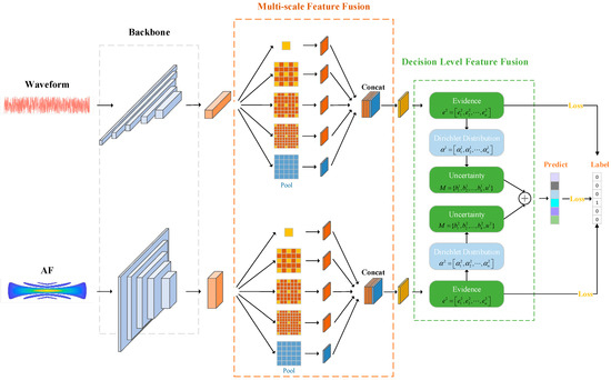
Figure 3.
The overall structure of MAFN.
- Multi-scale fusion module. The original waveform and the contour line of the AF are used as the input of this module. A backbone network is constructed to extract features from the multi-view input and then a multi-scale feature fusion layer is employed to fuse features from multiple scales of each view. Convolution kernels of different sizes are adopted in the multi-scale layer.
- Decision-level fusion module. A classifier follows the backbone and multi-scale feature fusion layers and then the predicted pseudo-labels of multi-view can be obtained. Then, the pseudo-label is assumed to be the Dirichlet distribution and the results of different views are dynamically integrated into the evidence layer via D-S evidence theory.
2.3. Multi-Scale Feature Fusion Module
In most of the CNNs for computer vision tasks, the convolution filters are often set as . They can only extract local features within the shift window, but not the global features. Unlike images in computer vision, it is important to capture the long-range spatial information in signals to improve the representation. Atrous Spatial Pyramid Pooling (ASPP) [25] can resample a given feature layer at multiple rates, which amounts to probing the signal with multiple filters that have complementary effective fields of view. However, the dilation rate in the original ASPP is too large, so, in our work, a modified ASPP is designed in the multi-scale feature fusion, with the parameters shown in Table 1. Among the five parallel sub-branches, the convolution layer is used to extract features, the dilated convolution is used to extract features at different scales, and the global pooling is used to extract global features. Finally, the features of the five sub-branches are concentrated at the channel level to obtain multi-scale features. This multi-scale feature fusion module can expand the receptive field without adding too many parameters.

Table 1.
The parameters of the modified ASPP.
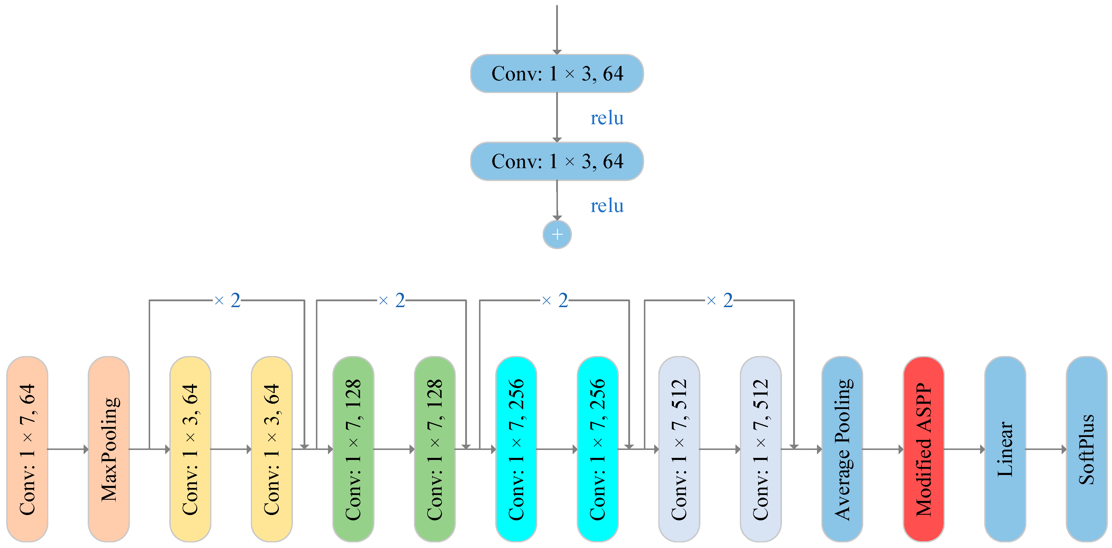
For the AF view, 2D ResNet18 [26] is adopted as the backbone. A ResNet-like 1D network is designed for the backbone of the original waveform view, as shown in Figure 4. The feature extraction part is followed by a fully connected layer to output a predicted label.

Figure 4.
Modified Resnet18 (1D and 2D) basic block and simplified structure.
2.4. Decision-Level Fusion Module
D-S evidence theory [27], introduced by A.P. Dempster and Shafer, provides a more general form of Bayesian inference and is proposed for imprecise inference. This theory allows the transformation of observed data into confidence and can be used for fusion at the decision level. It can discriminate uncertain information to ensure the confidentiality of the fusion. Decision-level fusion based on evidence theory involves two main processes, namely evidence construction and evidence combination. The construction of evidence involves the creation of mass functions to express uncertain data, while the combination of evidence involves the application of rules to determine the combination when the evidence is reliable or conflicting.
Definition 1
(Mass Function). Suppose represents the propositional space or the identification frame. Then, suppose there exists a mapping function from to [0, 1] that satisfies the following conditions
where m is defined as the mass function on the identification frame , or basic probability assignment (BPA). For , is the confidence value of proposition A, which indicates the degree of confidence that the evidence supports proposition A to be true. If , then proposition A is called the focal element and denotes the confidence value of propositions outside the identification frame .
Definition 2
(Confidence Function). Let A be a proposition on the identification framework . The confidence function is a BPA-based belief function that measures the degree of belief in proposition A. It is defined as the sum of the probabilities of all subsets of proposition A within the identification framework, expressed as
where is called the confidence level of proposition A, representing the degree of confidence that the evidence places in that proposition. This confidence level represents the minimum level of support for proposition A that can be inferred from the available evidence.
Definition 3
(Likelihood Function). The BPA-based likelihood function for proposition A on the identification framework is defined as the sum of the probabilities of propositions whose intersection with the proposition is not empty, expressed as,
where is commonly defined as the probability of proposition A, which reflects the degree of compatibility between the evidence and proposition A. It represents the maximum amount of support that the evidence can provide for proposition A. In the framework of evidence theory, the interval is used to represent the interval of uncertainty about the level of confidence in proposition A within the identification framework .
Definition 4
(Dempster Combination Rule). For , the two mass functions and on the identification framework , the combination rule for the focal elements and are
where is the conflicting term for the two mass functions, defined as
where [0, 1]. When , the two mass functions do not conflict completely; when , the two mass functions do not completely conflict; when , the combination rule fails.
Subjective logic (SL) [28] describes uncertainty in subjective knowledge by adding uncertainty to the notion of confidence. For the K classification problem, SL provides a theoretical framework to describe the uncertainty of an instance belonging to different classes based on the evidence learned in the data. For the vth view, denote the belief mass of an instance belonging to the kth category as , and denote the total uncertainty mass as . The relationship between the belief mass and the total uncertainty mass can be expressed as
Here the evidence is the output of the multi-scale feature fusion module, but it must be ensured that its value is not negative, denoted as
where is the input of the vth view, f corresponds to the backbone followed by a multi-scale feature fusion module and the classifier mapping function. For the vth view, an evidence vector is then formulated for the subsequent operations. It should be noted that the activation function takes the Softplus function with non-negative output. Thus, each value in the evidence vector satisfies .
In the context of multi-class classification, SL obtains the probabilities of different classes and the overall uncertainty by modeling the classification probability as Dirichlet distribution. Therefore, after obtaining the evidence vector for each view, according to the subjective logic theory, the parameters of the Dirichlet distribution can be expressed as
The belief mass and total uncertainty mass for each category are calculated as follows
where is the Dirichlet energy. From the formulas, we can see that, as the evidence value increases, the total uncertainty mass gradually approaches zero and, conversely, the uncertainty mass gradually approaches one. The belief mass and the overall uncertainty mass of all the categories are combined as . Assuming that there are views in total, several are cascaded as
Finally, the results of the different views have to be merged, using the Dempster combination rule as described in Equation (7). Since only two-view inputs are used in our network, . Then the fusion result of the two views is expressed as
where is used to balance the two confidence sets and the scale factor is used to normalize the output. From Equation (16), it can be seen that, when the uncertainties of the classification results from two views are high, the final classification result will have low confidence. When the uncertainties of the classification results from one view are low, the final classification result will have high confidence.
2.5. Loss Function and Learning Algorithm
When the number of categories is K, the support set of a K-dimensional Dirichlet distribution is a convex polyhedron containing K nodes in the K-dimensional space. While traditional neural networks often use Softmax as a non-linear activation function, the output of the network can be considered as a point on the simplex. In contrast, our method assigns a probability density to each point on the simplex via the Dirichlet distribution. Therefore, unlike the general cross-entropy loss, in our work the loss is calculated by integrating over the Dirichlet distribution and the result can be written as
where i is the sample index in the dataset, is the probability of assigning a class on a simplex, and is the logarithmic derivative of the gamma function. To obtain a large value at the correct class and a small value on the wrong class in the evidence vector for each sample, a KL divergence is added to the loss:
where is the fitting parameter of the Dirichlet distribution to avoid penalizing the evidence value at the correct category to 0 and is the gamma function. Combining Equation (17) and Equation (18), the final multilevel fusion loss formula is given by
where n denotes the number of samples, V denotes the number of views and is the balancing factor, which gradually increases with the number of iterations.
3. Experimental Results and Discussion
3.1. Datasets and Experimental Condition
In the experiment, we use two datasets to investigate the performance of the proposed MAFN, and the datasets are provided by the “Smart Eye Cup” competition (https://www.landinn.cn/project/detail/1629978822137, accessed on 10 February 2022). The first dataset is the navigation radar dataset which contains six types of radar emitters. The carrier frequency of the radar emitter signal is 100 MHz and the sampling frequency is 400 MSps. The second dataset contains twelve types of radar emitters. The carrier frequency of the radar emitter signals is 50 MHz and the sampling frequency is 200 MSps. Each radar radiation emitter contains 1000 sample files and the sequence length of each sample file is 420, so the dimensionality of dataset 1 is (6 × 000, 420) and the dimensionality of dataset 2 is (12 × 1000, 420). The modulation type of these radar emitters is QPSK. Three commonly used multi-classification metrics are used to evaluate the performance of REI methods: overall accuracy (OA), average accuracy (AA), and kappa coefficient (kappa). In the network training, we use the Adam [29] optimizer with an initial learning rate of 1 × 10⁻⁵ and the batch size is set to 32. The maximum number of epochs is set to 100. In all subsequent tests, 60% of the instances in each class are randomly sampled from the dataset used for the training, 10% of the instances in each class are randomly sampled from the dataset used for the validation, and the remaining 30% of the samples in each class are used for testing. To avoid randomness in the training, 30 experiments are run independently and the average results are calculated. All the experiments are run on a 64GB RAM HP Z840 workstation with two E5-2630v CPUs and an NVIDIA GeForce 3090 GPU.
3.2. Investigation on the Multi-View Representation
In this section we first validate the effectiveness of multi-view by comparing the proposed MAFN with two DNNs that deal with only one view, i.e., only the waveforms and only the AF. The two DNNs are denoted as View1-NF (View1—no fusion) and View2-NF, respectively. The one-view DNNs use the same network architecture as the algorithm proposed in this paper for a fair comparison, and the hyperparameters and network parameters are tuned to present the best classification results. The identification results of View1-NF, View2-NF, and MAFN on the two datasets are shown in Table 2.

Table 2.
The identification results of View1-NF, View2-NF, and MAFN on the two datasets.
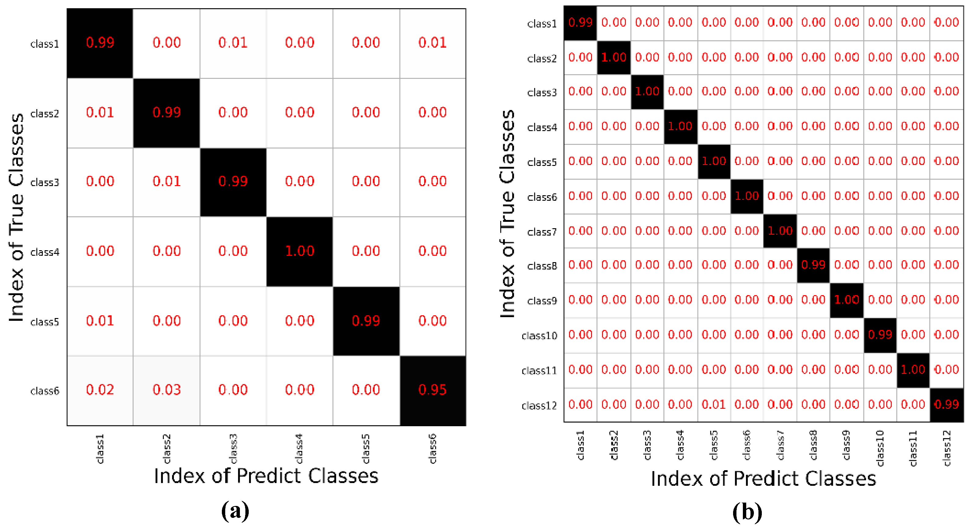
The results show that all three networks achieve high classification accuracy for the designed multi-scale layers. It is well known that a single-scale convolution kernel can only extract local features within a certain receptive field. In the multi-scale fusion module, by using different scales of convolutional kernels in the same view, local and global information in signals can be extracted separately and then fused more comprehensively for the final decision. By adaptively adjusting the weights for the fusion of different views, MAFN can provide more reliable results at the evidence level. Compared with the single-view networks without fusion strategy (View1-NF and View2-NF), the performance of MAFN with feature fusion is better in OA, AA, and kappa coefficients, which confirms the effectiveness of fusing multi-view information. The confusion matrixes of the classification results on the two datasets by MAFN are shown in Figure 5a,b, respectively.
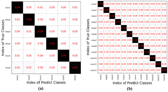
Figure 5.
Confusion matrix of MAFN. (a) Result on dataset 1. (b) Result on dataset 2. The column of the matrix represents the predicted class of samples, while the row represents the true class of samples. The numbers in the non diagonal element represent the incorrect recognition ratio. The numbers in the black background along the diagonal represent the correct recognition ratio of each class.
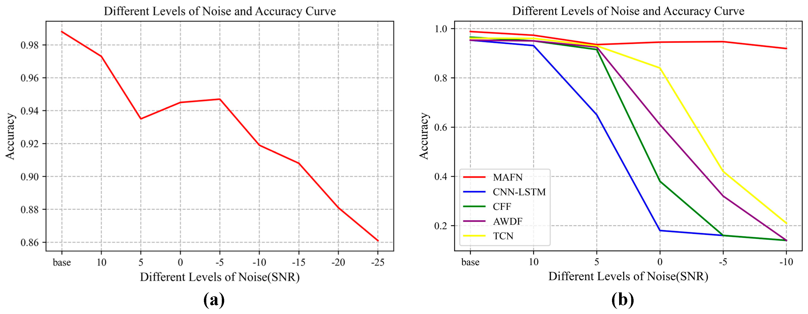
The robustness of REI is important in real applications because the assumptions of deep learning are so ideal that the model trained on the training set could not adapt well to the changing test set. To investigate the robustness of the proposed MAFN when the quality of the test data changes, dataset 1 is used as an example to add noise to the test. Gaussian noise is added to the signal to test the classification accuracy of the model. Signals with different SNRs are considered, ranging from −10 dB to 10 dB, and, in order to test the performance of our model in extreme scenarios, the lowest SNR is set to −25 dB. The quantitative results of the classification by MAFN are calculated. In addition, several related methods are compared with MAFN, including CFF [30] (feature-level stacked fusion method), adaptive weights decision fusion (AWDF) [31] (decision-level fusion method using adaptive weights), TCN [32], and CNN-LSTM [33] methods for REI. The experimental results of different networks are shown in Figure 6, where Figure 6a shows the variation of classification accuracy of our proposed algorithm MAFN with the SNR and Figure 6b shows the comparison results with other methods. By synthesizing multi-view information in the feature extraction for classification, MAFN is robust to signal degradation. From the results, we can observe a remarkable improvement of MAFN over other methods as the SNR decreases.

Figure 6.
The classification accuracy curves of MAFN and its counterparts under different SNRs. (a) Accuracy curve of MAFN with different SNRs. (b) Accuracy curve of comparison methods.
It should be noted that a slight fluctuation of the accuracy can be observed when the SNR takes the range of −5~5 dB when the results are amplified in Figure 6a. This phenomenon can be attributed to the random nature of the added noise, together with the intrinsic shortcoming of the gradient-based optimization algorithm. It is well known that, when training a DNN, the gradient-based algorithms can only guarantee to converge to a local optimum within a limited number of iterations. Therefore, for signals with random noise, there will be some small fluctuation in the classification results, especially when the energy of the signal and noise are comparable. Thus, in the range of [−5dB 5dB], we can observe some fluctuation within 1%. However, we can observe from Figure 6b that our proposed method has an improvement in recognition accuracy over other methods.
3.3. Investigation on the Multi-Scale and Fusion Module
3.3.1. Multi-Scale Module
In this section, we analyze the role of the multi-scale fusion module and the decision-level fusion module separately. First, the multi-scale feature fusion part is removed, and the results of different views go through the feature extraction backbone, the classification layer, and the decision-level fusion layer, which is denoted as MAFN-no M. The experimental results on dataset 1 and dataset 2 are shown in Table 3, from which we can observe that, on both datasets, the performance of the fusion network without the multi-scale feature fusion degrades.

Table 3.
Comparison of methods with/without multi-scale module on the two datasets.
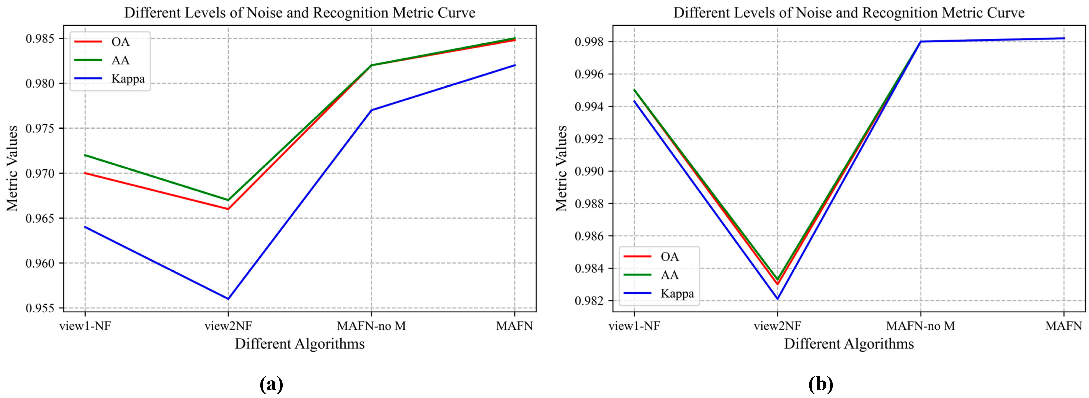
We also analyze the single-view network without the multi-scale feature fusion part. The no-fusion algorithm with only waveform as input (view1-no F), the no-fusion algorithm with only AF as input (view2-no F), and the multi-view algorithm without multi-scale feature fusion part, are compared with our proposed MAFN. The results on the two datasets are shown in Figure 1a and Figure 7b respectively. Figure 7a shows the OA, AA, and kappa coefficients of the four methods for dataset 1, and Figure 7b shows the OA, AA, and Kappa coefficients of the four methods for dataset 2. From the results, we can easily observe the performance improvement of decision-level fusion over the no-fusion algorithms, which confirms the effectiveness of multiple-views fusion.
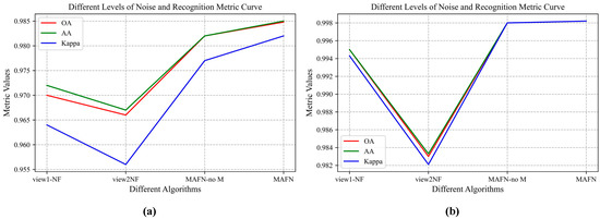
Figure 7.
Analysis of the multi-scale module. (a) Results on dataset 1. (b) Results on dataset 2.
3.3.2. Decision-Level Fusion Module
To validate the effectiveness of the decision-level fusion module, another fusion strategy, AWDF, is used to replace the evidence-level fusion strategy proposed in this paper for comparison. The multi-scale feature fusion part is the same as that of MAFN and, in this section, it is denoted as MAFN-no D. From the results we can observe that the adaptive weight decision-level fusion strategy is effective on both the datasets. Meanwhile, we compare the multi-view methods with the single-view methods. Here the method with only waveform and multi-scale feature fusion, denoted as View1-M, the method with only AF and multi-scale feature fusion, denoted as View2-M, and MAFN-no D are compared with our proposed MAFN. The experimental results on dataset 1 and dataset 2 are shown in Table 4. From this, we can observe the gain of both multi-scale feature fusion and decision-level fusion in REI.

Table 4.
Results of the strategies without decision-level fusion on the two datasets.
By a joint analysis of the experimental results in Table 2, we can observe that the multi-scale fusion strategy of the same view can also improve the recognition accuracy of single-view methods. By further introducing the adaptive weight fusion strategy, better results can be obtained from MAFN.
3.4. Comparison with Other Related Methods
In this section, we compare our method with some fusion-based REI methods, including the TWFF [34], a mean decision fusion (MDF) method [35], a simple cascade feature fusion (CFF) method, an adaptive weight decision fusion (AWDF) method, and the DSDF method [36]. CFF extracts the permutation entropy and sample entropy components of different eigenfunctions and fuses them in a cascade. TWFF dynamically adjusts the contribution of different views to the result during training by tuning the network parameters. The features of different views are fed separately to the convolutional neural network to compute the category probability of instances. MDF calculates the average of the outputs between different views to obtain the fusion output. AWDF trains a probabilistic support vector machine with different features separately and the recognition results are fused by adaptive weights to obtain the final results. DSDF inputs different views into a convolutional neural network and then the fusion results are obtained via the D-S evidence theory. We also compare the training and testing time of different methods. For DNNs, if the change of the loss function within 50 iterations is less than a given threshold, the network is considered to converge and the training time is calculated. We also test the inference speed of each method, by calculating the average inference time of 10,000 samples.
The comparison results on the two datasets are shown in Table 5. MAFN can extract different scale features of the same view and adaptively fuse the results of different views from a distributional perspective, thus avoiding incompatibility in fusing multi-view features. The results also show that the performance of the comparison methods is inferior to our proposed MAFN, including the feature-level fusion method, the fixed view weight method, the learnable weights method, and the voting method. As for the running time of the algorithms, CFF and AWDF have relatively high speed for using the SVM classifier. Compared with other DNNs, MAFN has medium speed for using multi-view inputs.

Table 5.
Comparison results of MAFN with other fusion algorithms (%).
4. Conclusions
In this paper, a multi-view adaptive fusion network (MAFN) is proposed by simultaneously exploring the signal waveform and the ambiguity function (AF). Experimental results show that the combination of multi-view features can provide spatially complementary information that improves the identification accuracy of radar emitters. Our experiments on two radar emitter datasets show that the proposed MAFN has some improvements over single-view networks, by synthesizing the signal waveform and AF. In addition, compared to single-view networks, MAFN is more robust to the distribution shift of the real radar emitter signals from the predefined training emitter signals, which also benefits from the fusion of multi-view features. Moreover, both the multi-scale feature extraction module and the decision-level fusion module are proven to extract more discriminative features of the signal, by exploring the Atrous Spatial Pyramid Pooling (ASPP) structure and the D-S evidence theory respectively. Compared with other related works, our proposed algorithm has a moderate computational complexity. However, when MAFN is used to recognize radar emitters in the case of very low SNR, its performance also degrades significantly. In addition, the network also requires a large number of labeled signal samples. In future work, we plan to design a self-supervised algorithm for REI with a very limited number of labeled signals [37] and improve the recognition accuracy when the SNR is extremely low.
Author Contributions
Conceptualization, S.Y. and Z.F.; methodology, H.L. and T.P.; software, H.L.; validation, T.P., H.L. and C.Y.; formal analysis, S.Y. and Z.F.; investigation, M.W.; resources, M.W.; data curation, M.W.; writing—original draft preparation, T.P.; writing—review and editing, S.Y.; visualization, T.P.; supervision, Z.F. All authors have read and agreed to the published version of the manuscript.
Funding
This work was supported by the National Natural Science Foundation of China (Nos. U22B2018, 61771376, 61771380, 61836009, 61906145); the Science and Technology Innovation Team in Shaanxi Province of China under Grant 2020TD-017; and partially by the Foundation of Intelligent Decision and Cognitive Innovation Center of State Administration of Science, Technology and Industry for National Defense, China; and the Key Project of Hubei Provincial Natural Science Foundation under Grant 2020CFA001, China.
Data Availability Statement
Not applicable.
Conflicts of Interest
The authors declare no conflict of interest.
References
- Saperstein, S.; Campbell, J.W. Signal Recognition in a Complex Radar Environment. Electronic 1977, 3, 8. [Google Scholar]
- Kawalec, A.; Owczarek, R. Radar Emitter Recognition Using Intrapulse Data. In Proceedings of the 15th International Conference on Microwaves, Radar and Wireless Communications (IEEE Cat. No. 04EX824), Warsaw, Poland, 17–19 May 2004; Volume 2, pp. 435–438. [Google Scholar]
- Ru, X.; Ye, H.; Liu, Z.; Huang, Z.; Wang, F.; Jiang, W. An Experimental Study on Secondary Radar Transponder UMOP Characteristics. In Proceedings of the 2016 European Radar Conference (EuRAD), London, UK, 5–7 October 2016; pp. 314–317. [Google Scholar]
- Zhao, Y.; Wui, L.; Zhang, J.; Li, Y. Specific Emitter Identification Using Geometric Features of Frequency Drift Curve. Bull. Pol. Acad. Sci. Tech. Sci. 2018, 66, 99–108. [Google Scholar]
- Cao, R.; Cao, J.; Mei, J.; Yin, C.; Huang, X. Radar Emitter Identification with Bispectrum and Hierarchical Extreme Learning Machine. Multimed. Tools Appl. 2019, 78, 28953–28970. [Google Scholar] [CrossRef]
- Chen, P.; Guo, Y.; Li, G.; Wan, J. Adversarial Shared-private Networks for Specific Emitter Identification. Electron. Lett. 2020, 56, 296–299. [Google Scholar] [CrossRef]
- Li, L.; Ji, H. Radar Emitter Recognition Based on Cyclostationary Signatures and Sequential Iterative Least-Square Estimation. Expert Syst. Appl. 2011, 38, 2140–2147. [Google Scholar] [CrossRef]
- Wang, X.; Huang, G.; Zhou, Z.; Tian, W.; Yao, J.; Gao, J. Radar Emitter Recognition Based on the Energy Cumulant of Short Time Fourier Transform and Reinforced Deep Belief Network. Sensors 2018, 18, 3103. [Google Scholar] [CrossRef]
- Seddighi, Z.; Ahmadzadeh, M.R.; Taban, M.R. Radar Signals Classification Using Energy-time-frequency Distribution Features. IET Radar Sonar Navig. 2020, 14, 707–715. [Google Scholar] [CrossRef]
- He, B.; Wang, F. Cooperative Specific Emitter Identification via Multiple Distorted Receivers. IEEE Trans. Inf. Secur. 2020, 15, 3791–3806. [Google Scholar] [CrossRef]
- Willson, G.B. Radar Classification Using a Neural Network. In Proceedings of the Applications of Artificial Neural Networks. In Proceedings of the 1990 Technical Symposium on Optics, Electro-Optics, and Sensors, Orlando, FL, USA, 16–20 April 1990; SPIE: Bellingham, WA, USA, 1990; Volume 1294, pp. 200–210. [Google Scholar]
- Shieh, C.-S.; Lin, C.-T. A Vector Neural Network for Emitter Identification. IEEE Trans. Antennas Propag. 2002, 50, 1120–1127. [Google Scholar] [CrossRef]
- Shmilovici, A. Support Vector Machines. In Data Mining and Knowledge Discovery Handbook; Springer: Berlin/Heidelberg, Germany, 2009; pp. 231–247. [Google Scholar]
- Sun, J.; Xu, G.; Ren, W.; Yan, Z. Radar Emitter Classification Based on Unidimensional Convolutional Neural Network. IET Radar Sonar Navig. 2018, 12, 862–867. [Google Scholar] [CrossRef]
- Zhu, M.; Feng, Z.; Zhou, X. A Novel Data-Driven Specific Emitter Identification Feature Based on Machine Cognition. Electronics 2020, 9, 1308. [Google Scholar] [CrossRef]
- Liu, Z.-M.; Philip, S.Y. Classification, Denoising, and Deinterleaving of Pulse Streams with Recurrent Neural Networks. IEEE Trans. Aerosp. Electron. Syst. 2018, 55, 1624–1639. [Google Scholar] [CrossRef]
- Notaro, P.; Paschali, M.; Hopke, C.; Wittmann, D.; Navab, N. Radar Emitter Classification with Attribute-Specific Recurrent Neural Networks. arXiv 2019, arXiv:1911.07683. [Google Scholar]
- Li, R.; Hu, J.; Li, S.; Ai, W. Specific Emitter Identification Based on Multi-Domain Features Learning. In Proceedings of the 2021 IEEE International Conference on Artificial Intelligence and Industrial Design (AIID), Guangzhou, China, 28–30 May 2021; pp. 178–183. [Google Scholar]
- Wu, B.; Yuan, S.; Li, P.; Jing, Z.; Huang, S.; Zhao, Y. Radar Emitter Signal Recognition Based on One-Dimensional Convolutional Neural Network with Attention Mechanism. Sensors 2020, 20, 6350. [Google Scholar] [CrossRef] [PubMed]
- Yuan, S.; Li, P.; Wu, B. Towards Single-Component and Dual-Component Radar Emitter Signal Intra-Pulse Modulation Classification Based on Convolutional Neural Network and Transformer. Remote Sens. 2022, 14, 3690. [Google Scholar] [CrossRef]
- Zhao, Y.; Wang, X.; Lin, Z.; Huang, Z. Multi-Classifier Fusion for Open-Set Specific Emitter Identification. Remote Sens. 2022, 14, 2226. [Google Scholar] [CrossRef]
- Yuan, S.; Li, P.; Wu, B.; Li, X.; Wang, J. Semi-Supervised Classification for Intra-Pulse Modulation of Radar Emitter Signals Using Convolutional Neural Network. Remote Sens. 2022, 14, 2059. [Google Scholar] [CrossRef]
- Stein, S. Algorithms for Ambiguity Function Processing. IEEE Trans. Acoust. Speech Signal Process. 1981, 29, 588–599. [Google Scholar] [CrossRef]
- Li, Y.; Yang, M.; Zhang, Z. A Survey of Multi-View Representation Learning. IEEE Trans. Knowl. Data Eng. 2018, 31, 1863–1883. [Google Scholar] [CrossRef]
- Chen, L.-C.; Papandreou, G.; Schroff, F.; Adam, H. Rethinking Atrous Convolution for Semantic Image Segmentation. arXiv 2017, arXiv:1706.05587. [Google Scholar]
- He, K.; Zhang, X.; Ren, S.; Sun, J. Deep Residual Learning for Image Recognition. In Proceedings of the IEEE Conference on Computer Vision and Pattern Recognition, Las Vegas, NV, USA, 27–30 June 2016; pp. 770–778. [Google Scholar]
- Shafer, G. A Mathematical Theory of Evidence; Princeton University Press: Princeton, NJ, USA, 1976; Volume 42, ISBN 0-691-10042-X. [Google Scholar]
- Jøsang, A. Subjective Logic; Springer: Berlin/Heidelberg, Germany, 2016; Volume 3. [Google Scholar]
- Kingma, D.P.; Ba, J. Adam: A Method for Stochastic Optimization. arXiv 2014, arXiv:1412.6980. [Google Scholar]
- Li, Y.; Jing, W.; Ge, P. Radiation Emitter Signal Recognition Based on VMD and Feature Fusion. Syst. Eng. Electron. 2020, 42, 1499–1503. [Google Scholar]
- Zhang, W.; Ji, H.; Wang, L. Adaptive Weighted Feature Fusion Classification Method. Syst. Eng. Electron. 2013, 35, 1133–1137. [Google Scholar]
- Jin, T.; Wang, X.; Tian, R.; Zhang, X. Rapid Recognition Method for Radar Emitter Based on Improved 1DCNN+TCN. Syst. Eng. Electron. 2022, 44, 463–469. [Google Scholar]
- Yin, X.; Wu, B. Radar Emitter Identification Algorithm Based on Deep Learning. Aerosp. Electron. Warf. 2021, 37, 7–11. [Google Scholar]
- Peng, S.; Zhao, X.; Wei, X.; Wei, D.; Peng, Y. Multi-View Weighted Feature Fusion Using CNN for Pneumonia Detection on Chest X-Rays. In Proceedings of the 2020 IEEE International Conference on E-health Networking, Application & Services (HEALTHCOM), Shenzhen, China, 1–2 March 2021; pp. 1–6. [Google Scholar]
- Jiang, W.; Cao, Y.; Yang, L.; He, Z. A Time-Space Domain Information Fusion Method for Specific Emitter Identification Based on Dempster–Shafer Evidence Theory. Sensors 2017, 17, 1972. [Google Scholar] [CrossRef]
- Zhang, Y. Research on Classification of Sensing Targets in Wireless Sensor Networks Based on Decision Level Fusion. Ph.D. Thesis, Beijing Jiaotong University, Beijing, China, 2019. [Google Scholar]
- Hao, X.; Feng, Z.; Yang, S.; Wang, M.; Jiao, L. Automatic Modulation Classification via Meta-Learning. IEEE Internet Things J. 2023. [Google Scholar] [CrossRef]
Disclaimer/Publisher’s Note: The statements, opinions and data contained in all publications are solely those of the individual author(s) and contributor(s) and not of MDPI and/or the editor(s). MDPI and/or the editor(s) disclaim responsibility for any injury to people or property resulting from any ideas, methods, instructions or products referred to in the content. |
© 2023 by the authors. Licensee MDPI, Basel, Switzerland. This article is an open access article distributed under the terms and conditions of the Creative Commons Attribution (CC BY) license (https://creativecommons.org/licenses/by/4.0/).


