Cloud Top Thermodynamic Phase from Synergistic Lidar-Radar Cloud Products from Polar Orbiting Satellites: Implications for Observations from Geostationary Satellites

Abstract

The cloud thermodynamic phase is a crucial parameter to understand the Earth’s radiation budget, the hydrological cycle, and atmospheric thermodynamic processes. Spaceborne active remote sensing such as the synergistic radar-lidar DARDAR product is considered the most reliable method to determine cloud phase; however, it lacks large-scale observations and high repetition rates. These can be provided by passive instruments such as SEVIRI aboard the geostationary Meteosat Second Generation (MSG) satellite, but passive remote sensing of the thermodynamic phase is challenging and confined to cloud top. Thus, it is necessary to understand to what extent passive sensors with the characteristics of SEVIRI are expected to provide a relevant contribution to cloud phase investigation. To reach this goal, we collect five years of DARDAR data to model the cloud top phase (CTP) for MSG/SEVIRI and create a SEVIRI-like CTP through an elaborate aggregation procedure. Thereby, we distinguish between ice (IC), mixed-phase (MP), supercooled (SC), and warm liquid (LQ). Overall, 65% of the resulting SEVIRI pixels are cloudy, consisting of 49% IC, 14% MP, 13% SC, and 24% LQ cloud tops. The spatial resolution has a significant effect on the occurrence of CTP, especially for MP cloud tops, which occur significantly more often at the lower SEVIRI resolution than at the higher DARDAR resolution (9%). We find that SC occurs most frequently at high southern latitudes, while MP is found mainly in both high southern and high northern latitudes. LQ dominates in the subsidence zones over the ocean, while IC occurrence dominates everywhere else. MP and SC show little seasonal variability apart from high latitudes, especially in the south. IC and LQ are affected by the shift of the Intertropical Convergence Zone. The peak of occurrence of SC is at −3 ${}^{\circ }$C, followed by that for MP at −13 ${}^{\circ }$C. Between 0 and −27 ${}^{\circ }$C, the occurrence of SC and MP dominates IC, while below −27 ${}^{\circ }$C, IC is the most frequent CTP. Finally, the occurrence of cloud top height (CTH) peaks lower over the ocean than over land, with MP, SC, and IC being undistinguishable in the tropics but with separated CTH peaks in the rest of the MSG disk. Finally, we test the ability of a state-of-the-art AI-based ice cloud detection algorithm for SEVIRI named CiPS (Cirrus Properties for SEVIRI) to detect cloud ice. We confirm previous evaluations with an ice detection probability of 77.1% and find a false alarm rate of 11.6%, of which 68% are due to misclassified cloud phases. CiPS is not sensitive to ice crystals in MP clouds and therefore not suitable for the detection of MP clouds but only for fully glaciated (i.e., IC) clouds. Our study demonstrates the need for the development of dedicated cloud phase distinction algorithms for all cloud phases (IC, LQ, MP, SC) from geostationary satellites.

1. Introduction

1.1. Background

Water in clouds in the Earth’s atmosphere is present as both liquid droplets and ice crystals. While the liquid phase exists at temperatures above 0 ${}^{\circ }$C and the ice phase at temperatures below the homogeneous nucleation threshold of about −40 ${}^{\circ }$C, both ice crystals and supercooled droplets can exist in the range between these two temperature thresholds as well as mixtures of them—known as mixed-phase. Knowledge about the occurrence of cloud phases—liquid (warm or supercooled), mixed-phase, or ice—is crucial for several reasons: Liquid clouds are made up of many small droplets, while ice clouds have significantly fewer, larger crystals. This results in liquid clouds being optically thicker and tending to have a stronger cooling effect on the atmosphere [1,2]. Furthermore, the phase of clouds impacts the absorption and scattering of incoming solar and emitted infrared radiation, particle evolution, and lifetime [3,4,5,6], and hence the cloud’s radiative effect [7,8,9,10,11]. Changes in cloud phase can lead to feedback impacting cloud fraction, humidity, and temperature profiles [9,12] as well as the formation of precipitation [13]. Moreover, aerosols impact thermodynamic phase change [14,15]. In order to better understand aerosol–cloud interactions a robust knowledge of the occurrence of different cloud phases is needed.

The thermodynamic phase transition of clouds is still not well understood, often leading to inaccurate representations of the distribution of ice and liquid in numerical models [10,13,16,17]. Mixed-phase clouds in particular are often poorly represented in global models as they tend to oversimplify the intricate microphysical processes that govern the transition between liquid and ice phases [4,10,18]. Constraining the phase transition mechanisms is particularly challenging since the physics and dynamics of mixed-phase clouds are nonlinear [10,19]. Numerous studies have also demonstrated the influence of cloud phase in climate sensitivity in general circulation models [16,20,21,22]. The phase partitioning of clouds and their parameterization are therefore of particular interest.

Satellite remote sensing is an important method to determine global cloud properties [23,24,25,26]. In recent years, spaceborne active remote sensing has been widely used to retrieve vertical profiles of thermodynamic cloud phases [10,27,28,29,30,31,32]. In particular, combinations of lidar and radar measurements provide a reliable way to determine the cloud phase, as both instruments complement each other due to their different penetration depths and different sensitivities to particle sizes [33,34,35,36]. For instance, the combined state-of-the-art CloudSat/CPR (Cloud Profiling Radar) and CALIPSO/CALIOP (Cloud-Aerosol Lidar and Infrared Pathfinder Satellite Observation/Cloud-Aerosol Lidar with Orthogonal Polarization) products have been used for statistical characterization of phase partitioning as well as statistics of the geographic and temporal occurrence of cloud phases [9,10,34,37,38].

Besides active instruments, passive sensors aboard geostationary satellites play an important role in observing the evolution and phase of clouds. Their main advantages are that, first, they provide information over a wide field of regard, which allows the retrieval of macrophysical quantities such as the sizes of clouds. Second, they allow measurements at any time of day, so that the temporal evolution of clouds can be studied with high temporal resolution. However, in contrast to active instruments, a passive sensor can only observe the upper layer of a cloud according to the penetration depth of its channels. For the evaluation of the radiative effect of a cloud, this cloud top layer is very important since it is where most solar radiation is reflected, and most infrared radiation is radiated to space [39]. Furthermore, since supercooled liquid and mixed-phase layers are usually located near the top of the cloud [40,41], they are expected to be observable with a passive instrument. In the past, phase retrievals of passive sensors often only distinguished between ice and liquid clouds (or ice/liquid/unknown) [42,43,44,45,46], but in recent years, retrieval algorithms for the imagers aboard the geostationary satellites GOES-R and Himawari have been developed to further distinguish between mixed-phase, liquid, and, for GOES-R, supercooled liquid cloud tops [25,47,48]. However, this distinction remains difficult, especially for mixed-phase and supercooled cloud tops [33]. For instance, the CiPS algorithm (Cirrus Properties from SEVIRI [49])—a neural network retrieval for the detection of ice clouds from SEVIRI aboard Meteosat Second Generation (MSG)—has been shown to (mis)classify supercooled clouds as ice clouds, especially when the temperature is close to the homogeneous nucleation threshold [50].

One of the difficulties in distinguishing between thermodynamic phases is that it cannot be performed on the basis of the cloud temperature alone, since ice, mixed-phase, and supercooled liquid clouds can all exist in the temperature range between 0 ${}^{\circ }$C and −40 ${}^{\circ }$C, as mentioned above. Distinguishing the cloud phase with passive sensors, therefore, requires additional consideration of radiative properties due to differences in absorption and scattering between liquid droplets and ice crystals [33,51]. However, cloud particles show large variations in habit and size and atmospheric conditions such as humidity or aerosol concentration and type can vary considerably in time and space. Moreover, the observed brightness temperatures and reflectivities are affected by other cloud and atmospheric properties as well as viewing geometry and, for reflectivities, by solar zenith angle. All these aspects make retrieval of the cloud thermodynamic phase a complex task. A further difficulty for passive instruments is that vertically thick clouds often consist of different thermodynamic phases in different layers. A passive sensor might receive signals from several of these layers, making classification difficult.

There are several studies on the geographic and temporal distribution of cloud phase from active spaceborne instruments [9,10,37,52]. However, results from these studies cannot be adopted one-to-one for passive geostationary satellites. Typically, studies using active remote sensing consider the total vertical profile of a cloud at a given time and location to define a phase for the cloud, while for passive, geostationary instruments, only the top layers of a cloud are relevant. Furthermore, passive, geostationary instruments usually have coarser resolutions, which has an influence on the cloud phases that fill the single pixels.

1.2. Scope of Present Work

Since, as outlined above, active spaceborne measurements constitute the most reliable way to determine the cloud phase from satellite observations, we use these measurements to determine a “ground truth” for cloud phase distributions from the perspective of a passive geostationary instrument. To this end, we use vertical profiles of the cloud phase from active remote sensing to model observations of the cloud top phase of a geostationary sensor. In particular, we use the spaceborne CALIPSO-CloudSat product DARDAR (liDAR/raDAR [53]) obtained with an along-track resolution of 1.1 km to deduce a cloud phase at cloud top as a ground truth for the MSG/SEVIRI geostationary passive instrument. Thereby we (1) restrict our analysis to the field of regard of SEVIRI (i.e., the Meteosat disk); (2) use the spatial resolution of SEVIRI (3 × 3 km${}^2$ at nadir, degrading towards the edge of the disk); (3) consider only the part of the cloud relevant for a passive sensor (mainly the upper layer); (4) aggregate DARDAR cloud phase results in every SEVIRI pixel to obtain a meaningful phase representation at SEVIRI resolution. This procedure results in an aggregated cloud top phase (CTP) in SEVIRI resolution—called “SEVIRI-like” CTP in the following. We test the influence of the resolution of SEVIRI on measurements of CTP by comparing the aggregated CTP in SEVIRI resolution with the corresponding CTP in DARDAR resolution, assessing how representative geostationary measurements of CTP are compared to measurements of polar-orbiting satellites. We confirm that the aggregation of the DARDAR cloud phase to the lower SEVIRI resolution preserves the relevant physical relationship between the SEVIRI-like CTP and temperature. To the best of our knowledge, the distribution of CTP derived from lidar/radar measurements as a “ground truth” has never been studied from the SEVIRI perspective—that is, at SEVIRI resolution and restricted to the top of the cloud. We fill this gap and study the geographic and seasonal distribution of the SEVIRI-like CTP. We also examine the differences between the various CTPs in terms of cloud top height (CTH), or more specifically, in which CTH regimes the CTPs occur. The results of these analyses can be used as a basis for testing and improving CTP determination algorithms for SEVIRI. Our approach allows us to assess the relative importance of liquid, ice, supercooled liquid, and mixed-phase cloud tops in SEVIRI observations at the spatial scale of the native SEVIRI grid. We focus in particular on the occurrence of mixed-phase and supercooled clouds. Since existing phase retrievals of passive sensors often are not able to detect these two cloud types as mentioned above, it is not a priori clear how many mixed-phase and supercooled clouds can be observed from a geostationary satellite. Furthermore, the SEVIRI-like CTP on the SEVIRI grid with variable pixel sizes can be interpreted in view of polar-orbiting active observations with constant along-track resolution. As a first application of the SEVIRI-like CTP data set, we evaluate the existing ice cloud retrieval algorithm for SEVIRI, CiPS (Cirrus Properties from SEVIRI).

Section 2 starts with an overview of the lidar-radar product DARDAR, the SEVIRI instrument, and CiPS. This is followed by the collocation and aggregation procedure of DARDAR and SEVIRI, yielding a data set containing CTP information in SEVIRI resolution. In Section 3, we study the influence of resolution on CTP observations and assess whether aggregating the DARDAR cloud phase to the lower SEVIRI resolution preserves physical relationships. We study the SEVIRI-like CTP as a function of different parameters such as geographical distribution, season, or land-ocean distribution. Finally, in Section 4, we compare the SEVIRI-like CTP with the ice cloud retrieval algorithm CiPS. We compute and assess the detection and false alarm rates of CiPS in order to better understand its strengths and weaknesses with respect to the detection of ice in the atmosphere as a preparation for a novel cloud retrieval development in the future.

2. Materials and Methods

2.1. DARDAR Data Set

As a ground truth for the occurrence of cloud phases, this study uses the DARDAR-MASK product which is part of the active remote sensing product DARDAR (liDAR/raDAR [53]). The DARDAR-MASK product is part of the Varcloud algorithm which was introduced by Delanoë and Hogan [35] and its cloud phase classification was further improved by Ceccaldi et al. [54]. It is based on the combination of active radar and lidar measurements from the A-Train satellites CloudSat and CALIPSO and provides a consolidated classification of the measured cloud scenes. DARDAR-MASK combines the sensitivity of lidar to optically thin cirrus with the capability of radar to penetrate optically thicker clouds. Due to this unique approach, these products have been widely used for cloud studies [9,37,55,56,57].

The DARDAR-MASK data set provides vertical profiles of cloud thermodynamic phase collocated with CloudSat footprints with a spatial resolution of 1.1 km along and 1.7 km across the satellite track and a 60 m vertical resolution. Single measurements of 1.1 km × 60 m boxes are called gates in the following to avoid confusion with SEVIRI pixels. The product consolidates the CALIPSO Level 1B profiles of attenuated backscatter coefficient, $\beta$, at 532 nm and the CloudSat 2B-GEOPROF radar reflectivity at 94 GHz, Z, with the CALIPSO Lidar L2 Vertical Feature Mask (VFM) using a decision tree to obtain phase discrimination for optically thin and thick clouds. In the improved DARDAR-MASK version (v2.23), histogram-adapted thresholding is directly applied to the original lidar data of $\beta$ at 60 m vertical resolution to identify atmospheric targets such as clouds or aerosols. After the feature detection, the VFM mask is used to filter out aerosols. Subsequently, remaining atmospheric targets are labeled as warm liquid clouds where the wet bulb temperature is >0 ${}^{\circ }$C which is calculated from temperature, pressure, and humidity from the ECMWF-AUX data set [58]. In addition, cloud layers containing supercooled water are singled out using their strong lidar backscatter and subsequent attenuation in temperature regions between 0 ${}^{\circ }$C and −40 ${}^{\circ }$C. A further distinction into pure supercooled water without ice crystals is made using the absence of a radar return since the diameter of cloud droplets is mostly below the CloudSat sensitivity [59]. Below −40 ${}^{\circ }$C, these layers with strong backscatter are attributed to highly concentrated ice. If the layer is thicker than 300 m in the 0 ${}^{\circ }$C to −40 ${}^{\circ }$C temperature range, it is assumed to be fully glaciated which is in line with observations [30] and modeling studies [60]. The same applies to atmospheric targets which are not labeled as aerosols in temperature regions below −40 ${}^{\circ }$C. Further sub-divisions are made for spherical ice or 2D plates using their low depolarization and for regions above convective cores. Details regarding this phase discrimination technique can be found in [54]. The DARDAR product also contains temperature profiles taken from the ECMWF-AUX data set, which are interpolated to DARDAR resolution [53]. We use these temperature profiles to determine a cloud top temperature (CTT) for each cloudy DARDAR profile. For this, we select the temperature in the top cloudy gate as CTT. Similarly, we define a cloud top height (CTH) as the height of every topmost cloudy gate in each cloudy DARDAR profile.

In the following, we use the DARMASK_Simplified_Categorization data set contained in the DARDAR-MASK (v2.23) product which comprises: four ice categories (ice, spherical or 2D ice, highly concentrated ice, top of convective towers) that we consider as “ice”; one category for mixtures of supercooled liquid and ice (supercooled+ice) that we consider as “mixed-phase”; two “pure” supercooled categories (supercooled, multiple scattering due to supercooled water) that we consider as “supercooled”; four liquid categories (liquid, warm rain + liquid clouds, cold rain + liquid clouds, rain maybe mixed with liquid) that we consider as “liquid” in the following. Thus, we distinguish between ice (IC), mixed-phase (MP), supercooled (SC), and warm liquid (LQ) cloud classes. We refer to these four classes in the following as phases for simplicity, although SC and LQ have the same thermodynamic phase (liquid) and MP contains water in two thermodynamic phases (solid and liquid). Note that we ignore other classifications included in DARDAR-MASK such as aerosols or stratospheric features for the cloud phase classification and treat them as clear sky.

Figure 1a gives an example of the Simplified Categorization variable of the DARDAR-MASK product for an A-Train curtain on 10 June 2015 at 12:15 UTC. The scene shows a cross-section through a stationary occlusion front located just west of Norway. With an overcast ice cloud layer in the lifted warm sector, mixed-phase clouds with embedded supercooled layers run ahead of the front, while a low and supercooled layer is trailing the front in the cold sector.

2.2. MSG and CiPS

The MSG satellites have been operational since 2004 and are positioned at 0${}^{\circ }$E above the equator. SEVIRI has a spatial coverage from approximately 80${}^{\circ }$W to 80${}^{\circ }$E and 80${}^{\circ }$S to 80${}^{\circ }$N, covering the African and European continent as well as large parts of the Atlantic ocean. Apart from one high spatial resolution visible (HRV) channel, the imager has 11 channels between 0.6 and 14 μm with a spatial resolution of $3\times 3$ km${}^2$ at nadir and a temporal resolution of 15 min.

In Section 4, we use the aggregated SEVIRI-like CTP data set to evaluate the CiPS (Cirrus Properties from SEVIRI) algorithm. CiPS detects ice clouds, even in multilayered situations with lower “warm” clouds, and retrieves the corresponding CTH, ice optical thickness, and ice water path using the SEVIRI imager. The algorithm utilizes a set of artificial neural networks trained with MSG2/SEVIRI thermal observations, CALIOP L2 cloud and aerosol layer data version 3 (V3) with a spatial resolution of 5 km (CAL_LID_L2_05kmC|ALay-Prov-V3-0X [61]; abbreviated with CAL_LID_L2 in the following), surface temperature from ECMWF (ERA-Interim reanalysis) and auxiliary data over a time period of almost six years from April 2007 to January 2013 [49]. CiPS has been extensively validated [50]: it detects approx. 70% of the ice clouds with an optical thickness of 0.1, and this value increases rapidly with increasing optical thickness. According to [50], CiPS shows an overall probability of detection (POD) of 70% over the entire disk and a false alarm rate (FAR) of 4%, with the highest values of the FAR in the tropics and smallest values in mid-latitudes. Furthermore, CiPS has been shown to partly identify supercooled tops wrongly as ice, with FAR increasing with decreasing temperature: while only 6% of liquid tops are classified by CiPS as ice between −10 and −15 ${}^{\circ }$C, this fraction increases to 35% for temperatures between −30 and −35 ${}^{\circ }$C. Like the training of CiPS, the evaluation has been performed against CAL_LID_L2, which distinguishes “only” between the phases ice, liquid water, and undetermined.

2.3. Definition of the Cloud Top Phase

In the following sections, we explain the procedure to derive the SEVIRI-like CTP from the DARDAR-MASK product. Roughly summarized, the vertical profiles of the DARDAR product—which have a higher resolution along the track than the size of one SEVIRI pixel—are mapped to a one-dimensional CTP variable in the spatial resolution of SEVIRI (from now on called SEVIRI resolution). Note that the DARDAR data are always collected at the time of the overpass of the satellites CALIPSO and CloudSat. The frequency of occurrence of the deduced CTP can therefore only be representative of the respective overflight times for each location.

Figure 1b shows a (fictitious) DARDAR-MASK scene with clouds with different thermodynamic phases. The vertical black lines indicate the geostationary grid of SEVIRI. The horizontal bar above the DARDAR-MASK scene shows the resulting CTP in SEVIRI resolution after the vertical and horizontal averaging steps. These steps are explained in detail below.

2.3.1. Removal of Isolated Gates

The DARDAR algorithm sometimes identifies isolated gates as cloudy, typically classified as supercooled. It can be assumed that these isolated cloud gates are in most cases not physically meaningful but noisy artifacts of the lidar cloud mask algorithm and, due to their size, can never fill a SEVIRI pixel. Before regridding the DARDAR data to the coarser MSG resolution, these isolated cloud gates are filtered out from the two-dimensional DARDAR-MASK. Isolated cloud gates here refer to cloudy gates that have only non-cloudy gates as direct neighbors in a square of $3\times 3$ gates (see Figure 1b).

2.3.2. Identification of the Cloud Top Layer

Radiation measured by passive instruments does not only stem from the very top of a cloud but some vertical extent of the cloud top layer (e.g., [62]). To account for this fact, we do not consider only the topmost cloudy gate in the DARDAR product but a vertical band of four cloudy DARDAR gates (i.e., 240 m) starting from cloud top is used in the CTP definition (black dashed line in Figure 1b). Taking several vertical layers into account better represents clouds that have a mix of very thin layers (1–3 gates) of different phases at the cloud top from the point of view of passive imagers: A typical case is clouds with an MP or SC very thin vertical layer at the cloud top with IC underneath. Examples can be seen in Figure 1a at longitudes between about 0.5 and 1.0${}^{\circ }$E, where very thin SC layers are at cloud top with MP and IC layers underneath. For LQ and IC clouds (thin/thick cirrus, but not convective), that have the same phase over a large vertical extent, the consideration of these four gates below the cloud top has the same effect as considering the topmost gate alone. Finally, we consider cloudy gates to belong to different cloud layers when there is a vertical cloud gap of at least 2 km between them. For these multilayered clouds, e.g., a high IC cloud layer on top of lower clouds, we only consider the gates within the uppermost cloud layer (even if its geometrical thickness is thinner than 240 m). Although radiation from the lower cloud layer can be transmitted through the higher cloud and affect the satellite observation, this procedure ensures that we focus on the cloud that is closest to the satellite. Furthermore, this is consistent with the conventions of the CiPS algorithm [49] which will be evaluated in Section 4.

A more physical approach to identify the vertical layer that is most relevant to the passive spaceborne observations would be to calculate a vertical penetration depth as a function of the extinction coefficient of the clouds. However, in the absence of information about the extinction coefficient—which, by the way, is also wavelength dependent—for all cloud phases, a reasonable solution is to use a fixed vertical band. The value of 240 m for the vertical extension of the cloud top layer is a compromise to choose the vertical band thick enough to consider the presence of several thin vertical layers of different phases at the cloud top, which should be counted as MP, and thin enough to not give too much weight to lower layers that are too far away from cloud top. This is most important for clouds with SC layers at the top that are usually smaller than 300 m (see Section 2.1). This is shown schematically in Figure 1b, where the vertical band indicated by the black dashed line is thinner than the typical thickness of MP and SC layers at the cloud top, but includes most of the gates associated with these phases. Note that the scope of the work is not to study the effective phase for SEVIRI from which the radiation in the cloud originates, but to perform statistical studies for the dominant phase at the geometrical cloud top. We further discuss the influence of the choice of 240 m as the thickness of the vertical band in Appendix A.

2.3.3. Collocation and Aggregation

The SEVIRI-like CTP is defined as the aggregation of all DARDAR values mapped to a SEVIRI pixel which are included in the vertical band defined in the previous section, i.e., all DARDAR values contained in the two-dimensional stripe below the cloud top. The procedure works in the following manner.

• The DARDAR profiles are collocated with SEVIRI pixels based on latitude, longitude, acquisition time, and CTH information of the topmost gate (see Figure 1b). Consideration of the CTH is needed since a DARDAR gate containing a high cloud can be assigned to a different SEVIRI pixel than suggested by the longitude and latitude due to the viewing angle of the geostationary satellite (parallax effect).
• If no cloudy gates are present, the SEVIRI pixel is classified as clear-sky.
• A cloudy pixel in SEVIRI resolution is required to contain only DARDAR gates that have a similar CTH. Otherwise the averaging might take place over two different clouds. Therefore, all SEVIRI pixels for which the CTHs of any of the contained DARDAR gates vary by more than 1 km are not considered further.
• If a SEVIRI pixel is not fully covered by cloudy DARDAR gates, it is not considered further in order to avoid cloud edges.
• If a SEVIRI pixel is fully covered by cloudy DARDAR layers, the CTP is assigned by considering all DARDAR gates included in the vertical band mentioned above:
  • If all DARDAR gates are of the same phase, the SEVIRI-like CTP adopts this phase classification.
  • SEVIRI pixels which contain different DARDAR cloud phases, but only the phases IC, MP, or SC are classified as MP cloud tops.
  • SEVIRI pixels that contain LQ and at least one more phase (IC, MP, or SC) are not considered further; this applies to edges between LQ clouds and clouds with other phases.

This way, a data set of SEVIRI-like CTP can be created with homogeneous pixel properties that give information about the presence of ice alone, warm liquid droplets, or supercooled liquid particles alone or mixed with ice crystals. Notice that the last case encompasses the mixed-phase cloud situation where ice and liquid are mixed at the microphysical level [63], but also the case where ice (or MP) and liquid are next to each other inside one MSG pixel.

For the analysis of the influence of the resolution on CTP (see Section 3.1), we also define a CTP in DARDAR resolution (DARDAR-CTP). The DARDAR-CTP is obtained by the same steps as described above (i.e., defining a vertical band at the cloud top and aggregating the phase values of this band to a CTP value), except for the horizontal aggregation to SEVIRI resolution. Hence, the only difference between the SEVIRI-like CTP and DARDAR-CTP is their different horizontal resolutions.

2.4. Data Set of Collocated DARDAR and MSG Cloud Top Phase

Following the steps defined above, the SEVIRI-like CTP and DARDAR-CTP are computed for the five years 2013–2017. We selected this time period because it has the longest overlap with a consistent operational MSG satellite (MSG3) and DARDAR data that was available to us at the time we conducted this study. Furthermore, concentrating on MSG3 prevents us from using observations with high aerosol load due to the volcanic eruptions in 2010 and 2011 (Eyjafjallajökull, Grimsvötn, Puyehue) that affect passive observations.

The SEVIRI-like data set is complemented with two other variables from the DARDAR data set: CTT and CTH. CTT at SEVIRI resolution is determined as an average over all CTTs at DARDAR resolution (Section 2.1) inside a given SEVIRI pixel. Similarly, CTH, which is computed for every topmost cloudy gate in DARDAR (see Section 2.1), is averaged over all cloud tops inside a SEVIRI pixel. Overall, the five years of data in SEVIRI resolution amount to roughly 77 × 10${}^6$ data points. Since CloudSat was working in daylight-only mode, no data is collected during overflights of the Antarctic in southern winter, which results in fewer data points over the Antarctic compared to other regions.

As an additional parameter, the land-sea-mask from ERA5 [64] is used. The ERA5 land-sea-mask has an original resolution of ${0.25}^{\circ }\times {0.25}^{\circ }$ in longitude and latitude which is coarser than the SEVIRI resolution. Regridding to the SEVIRI resolution is performed using the nearest neighbor algorithm.

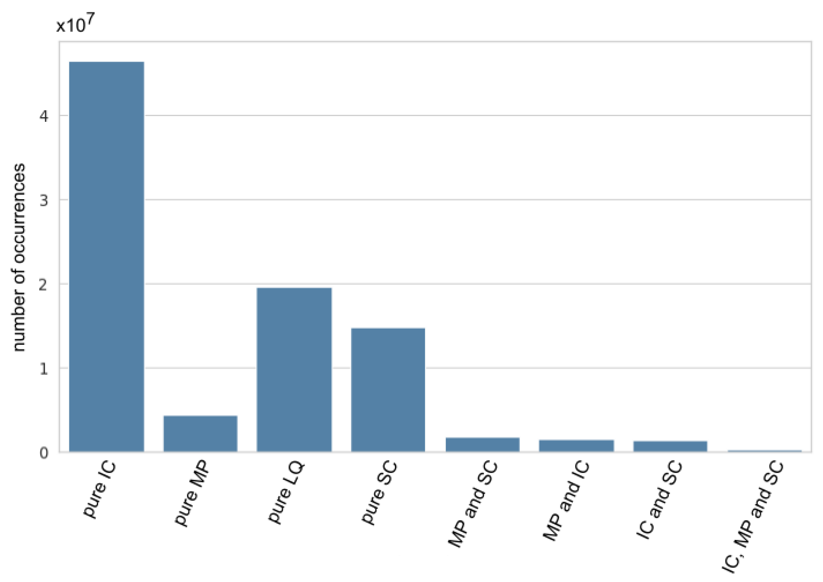
3. Occurrence of Cloud Top Phase

In this section, we analyze the statistics of the five years of CTP (Section 2.3). First, we analyze the influence of the resolution of the instruments by comparing the CTP in DARDAR resolution with the lower resolution SEVIRI-like CTP (Section 3.1). Next, we assess whether aggregating the DARDAR CTP to the lower SEVIRI resolution preserves relevant physical relationships by studying the distribution of SEVIRI-like CTP as a function of CTT (Section 3.2). Finally, we study the geographic distribution, seasonal variability, and altitude of the SEVIRI-like CTP (Section 3.3 and Section 3.4).

3.1. Resolution Effects and Geographic Distribution

We analyze the influence of the resolution on CTP by comparing the SEVIRI-like CTP to the DARDAR-CTP. In order to study the differences between the CTPs in different resolutions, $Rϵ$ {SEVIRI, DARDAR}, and their geographical distribution, we define a set of variables on a common grid. As in other publications dealing with the sparse active observations by CALIPSO-CloudSat (e.g., [10]), we select boxes of 2.5${}^{\circ }$ latitude by 2.5${}^{\circ }$ longitude over the MSG disk. The size of the latitude-longitude boxes is chosen to obtain good statistics and still show all the important features of the cloud phases on the Meteosat field of regard. Notice that differences are given in this investigation only by the filtering-averaging-aggregation procedure implemented in Section 2.3 and not to orbital parameters since all values are determined along the satellite track of CALIPSO-CloudSat. Notice that the procedure applied in Section 2.3 both modifies the occurrence of the single phases as well as the number of cloudy “observations” because of downscaling (averaging) but also because of the removal of inhomogeneous pixels. This removal of inhomogeneous pixels, i.e., pixels that are either not fully covered with cloudy gates or that contain clouds with large CTH differences (see Section 2.3), is depicted in Figure 2a. It shows the percentage of SEVIRI pixels per latitude-longitude grid box which are omitted. This percentage of omitted pixels is small in general (≲20%), but it is higher on the one hand in regions where many small clouds (with a spatial extent smaller than a SEVIRI pixel) are present, such as cumulus clouds over subtropical oceanic regions, leading to partly covered pixels. On the other hand, the percentage is higher where many multi-layered clouds with large CTH differences are present, such as at the borders of the Intertropical Convergence Zone (ITCZ) with high anvil cirrus clouds over low clouds. Figure 2b shows the number of data points of the SEVIRI-like CTP data set per latitude-longitude grid box. The derived data set contains on average about 10${}^4$ SEVIRI-like pixels per grid box and thus enough data for robust statistics. The inhomogeneous spatial distribution of the number of data points on the Meteosat disk is the result of several factors, such as the increasing size of SEVIRI pixels with distance from nadir, the fact that the flight path of CALIPSO/CloudSat passes over some SEVIRI pixels more frequently than others, and the seasonally changing coverage of CALIPSO/CloudSat in daytime mode.

To study the differences between CTPs at different resolutions and their geographic distribution, we define the cloudiness—i.e., the probability that a geographic box is cloudy—$P_R\left(\mathrm{cloud}\right|\mathrm{lat},\mathrm{lon})$, and the phase occurrence—i.e., the probability that a given phase occurs in a geographic box—$P_R\left(q\right|\mathrm{lat},\mathrm{lon})$ with $qϵ$ {IC, MP, SC, LQ} in each latitude-longitude grid box according to

$$P_R\left(q\right|\mathrm{lat},\mathrm{lon})=\frac{N_R(q,\mathrm{lat},\mathrm{lon})}{N_R\left(\mathrm{cloud},\mathrm{lat},\mathrm{lon}\right)},$$

(1)

$$P_R\left(\mathrm{cloud}\right|\mathrm{lat},\mathrm{lon})=\frac{N_R\left(\mathrm{cloud},\mathrm{lat},\mathrm{lon}\right)}{N_R\left(\mathrm{lat},\mathrm{lon}\right)},$$

where (lat, lon) label the latitude-longitude box, $N_R(q,\mathrm{lat},\mathrm{lon})$ is the number of data points in the box with CTP q, $N_R\left(\mathrm{cloud},\mathrm{lat},\mathrm{lon}\right)$ is the number of cloudy data points in the box, i.e., $N_R\left(\mathrm{cloud},\mathrm{lat},\mathrm{lon}\right)={\sum }_q{N}_R(q,\mathrm{lat},\mathrm{lon})$ and $N_R\left(\mathrm{lat},\mathrm{lon}\right)$ is the total number of data points in the box. From the definition of $P_R\left(q\right|\mathrm{lat},\mathrm{lon})$, it follows that the sum over all CTPs q gives 1.0 at every latitude and longitude grid box.

Figure 3 shows the cloudiness and phase occurrence for SEVIRI and DARDAR resolution, respectively, in the left and middle columns. The right column shows the difference between SEVIRI and DARDAR resolution for cloudiness and phase occurrence. The number at the top right corner of each plot is the respective mean value over all latitude-longitude boxes. Comparing the plots at SEVIRI and DARDAR resolution, one first sees that the main characteristics of the geographic distribution of cloudiness and phase occurrence of each CTP are preserved in the aggregation procedure from DARDAR to the coarser resolution of SEVIRI.

The highest cloudiness values are found over the Southern Ocean and high northern latitudes over the ocean in both resolutions with cloudiness values up to 97%. In fact, the Southern Ocean and the Antarctic seas have the largest cloud fractions as already demonstrated in previous studies using other synergistic A-Train products [37,65,66,67,68,69,70]. In the tropics near the equator, cloudiness values are also enhanced compared to the average value on the Meteosat disk because of frequent convection. The lowest cloud probabilities occur close to the Tropic of Cancer and Tropic of Capricorn over land, in the subsidence regions.

All CTPs shown in Figure 3b–e have a strong geographic dependence. IC cloud tops are the most common cloud phase with a mean phase occurrence of 49% (50%) in SEVIRI (DARDAR) resolution. They occur over the whole Meteosat disk, but are most probable at high latitudes in the temperate zones as well as in the ITCZ and the African continent. LQ cloud tops are mainly found in the subtropics and over the ocean rather than on land. The process leading to the high occurrence of LQ cloud tops in these regions is shallow convection, which is typical for regions with high solar irradiation and abundant moisture from the ocean. The highest probabilities for LQ cloud tops (over 90% in both resolutions) are found over the ocean west of the African continent related to low stratocumulus clouds, which are very common in this region. Their probability of occurrence becomes smaller towards high latitudes N or S. In particular, LQ cloud tops are almost never observed at latitudes south of 60${}^{\circ }$S. MP and SC cloud tops on the other hand are most frequently observed at high latitudes north of 60${}^{\circ }$N or south of 60${}^{\circ }$S. SC cloud tops are especially prevalent over the Southern Ocean with mean values of about 30% in SEVIRI resolution and 35% in DARDAR resolution for latitudes south of 60${}^{\circ }$S.

Even if the general patterns of CTP are similar in both resolutions, significant differences in phase occurrence between SEVIRI and DARDAR resolutions are also found. For MP cloud tops in SEVIRI resolution, relatively high values of over 10% extend into the temperate zones, the Southern Ocean, Europe, and the northern Atlantic and are therefore well visible within the Meteosat disk. In contrast, MP cloud tops in DARDAR resolution are less common. As can be seen from the difference between SEVIRI and DARDAR resolution results for MP cloud tops in Figure 3c, MP phase occurrence is higher in SEVIRI resolution everywhere on the Meteosat disk. While in SEVIRI resolution the mean value of MP phase occurrence is 14%, only 9% of clouds are MP in DARDAR resolution. The MP values in SEVIRI resolution are, in some regions (e.g., over Scandinavia, South Africa, or the central parts of the Southern Ocean), almost twice as high as in DARDAR resolution. These differences in the two resolutions are explained by the aggregation of different cloud phases in DARDAR resolution within a SEVIRI pixel: when DARDAR gates of more than one “cold” phase (IC/MP/SC) are present in a SEVIRI pixel, they are aggregated and contribute to the MP CTP in SEVIRI resolution (see Section 2.3). Physically, this corresponds to the mixing of clouds of different phases within a SEVIRI pixel such that, e.g., an SC cloud top contiguous to an IC cloud top in one SEVIRI pixel cannot be distinguished from an MP cloud top that extends over the whole SEVIRI pixel. Accordingly, IC and SC phase occurrences are lower in SEVIRI resolution compared to DARDAR resolution, in the same regions where MP phase occurrence is higher in SEVIRI resolution (see Figure 3b,e).

A second mechanism—besides aggregation—that causes differences between the phase occurrences in the two resolutions is that DARDAR results are not used and the corresponding SEVIRI pixels are omitted if they are either not fully covered with cloudy gates or if there are too large CTH differences (see Section 2.3 and Figure 2a).

In the phase occurrence probabilities, we see these differences due to non-fully covered pixels and cloud edges mainly in the IC and LQ CTPs in Figure 3b,d. The LQ phase occurrence is smaller for the SEVIRI resolution than for the DARDAR resolution. The reason is that when small-scale LQ clouds, which do not fully cover SEVIRI pixels, are omitted in SEVIRI resolution, the number of LQ data points decreases. As a consequence, the phase occurrence for LQ cloud tops decreases (see Equation (1)). This can be seen in Figure 3, as the difference between the SEVIRI and DARDAR resolutions for the LQ phase occurrence shows a similar pattern on the Meteosat disk as the percentage of SEVIRI pixels omitted.

Omitting DARDAR LQ values, which do not fully cover SEVIRI pixels, in going to SEVIRI resolution also has consequences for the IC phase occurrence. Comparing the differences between SEVIRI and DARDAR resolution for IC and LQ CTPs, we find higher values of IC phase occurrence in SEVIRI resolution compared to DARDAR resolution in the same spatial pattern as lower LQ phase occurrence values (see Figure 3b,d). This is explained by the following argument: Assuming a fixed number of IC data points, omitting LQ data points in going from DARDAR to SEVIRI resolution results in a decrease in the total number of cloudy data points and therefore an increase in the IC phase occurrence (see Equation (1)). Hence, a lower SEVIRI LQ phase occurrence compared to DARDAR is compensated by an increase in SEVIRI IC phase occurrence. This also holds for SC and MP cloud tops. However, from the phase occurrence plots in Figure 3b–e, one can see that SC and MP phase occurrence are low compared to the other two phases in the regions where we find differences between the two resolutions for LQ phase occurrence.

MP and SC cloud tops typically occur in mid and high latitudes as large and persistent boundary layer stratiform clouds [33]. Usually, there are no other clouds above these stratiform clouds and they can be well observed from a geostationary satellite. Therefore, pixels containing MP and SC cloud tops in SEVIRI resolution are rarely omitted, as can be seen in the distribution of the percentage of omitted SEVIRI pixels in Figure 2a.

Summarizing, all four CTPs occur in significant amounts in the SEVIRI-like CTP data set: The mean over all grid boxes is larger than 10% for all phases in SEVIRI resolution. The resolution influences the phase occurrences significantly: MP cloud tops are significantly more frequent (mean values of 14% vs. 9%), while SC and IC cloud tops are less frequent in the lower SEVIRI resolution compared to the higher DARDAR resolution. The effects of non-fully covered pixels and edges between clouds mainly influence the occurrence of LQ and IC cloud tops in the SEVIRI-like data set. As a consequence, LQ cloud tops appear less often in SEVIRI than in DARDAR resolution, while the probability for IC cloud tops rises in the same regions.

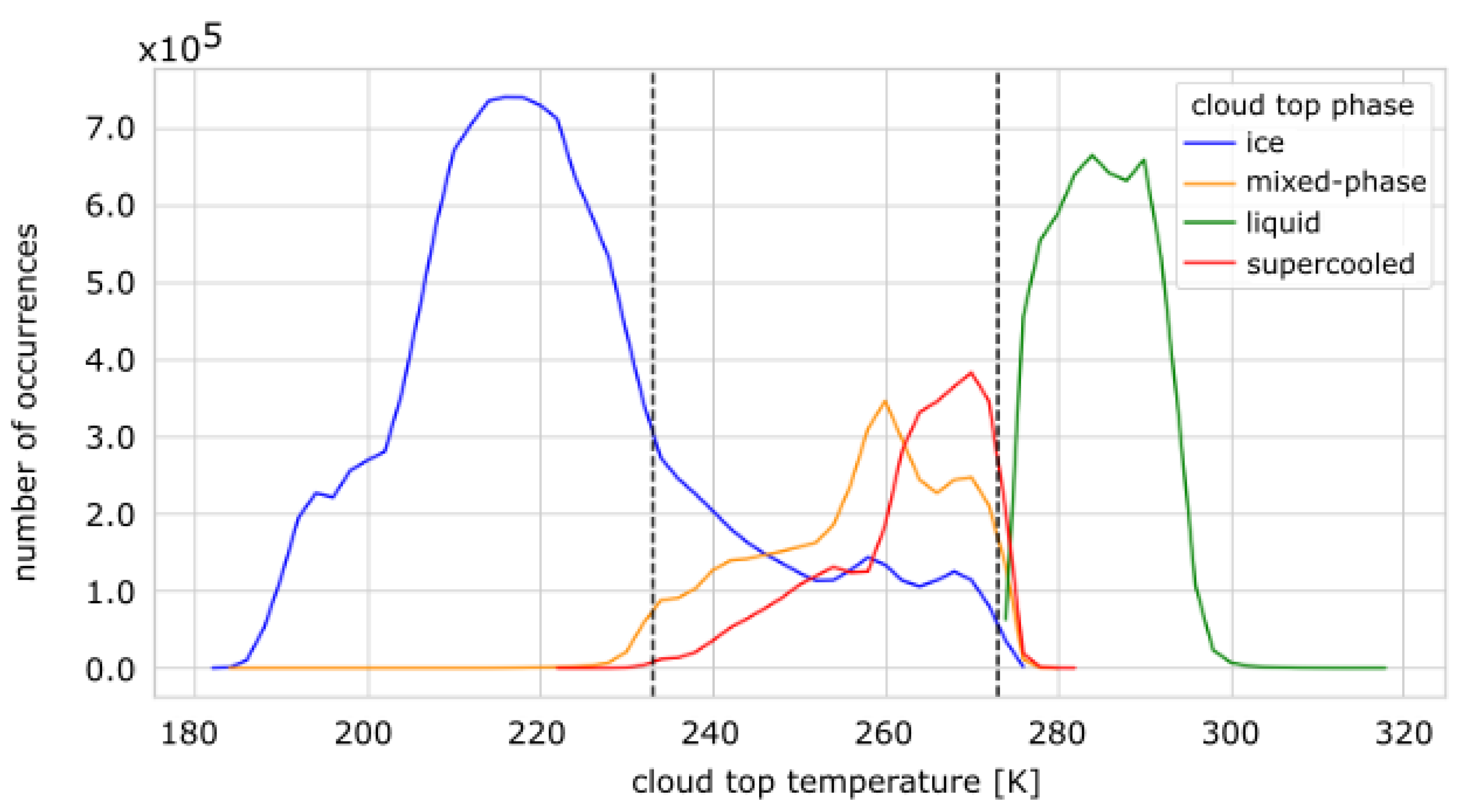
3.2. Phase as a Function of Cloud Top Temperature

Figure 4 shows the number of occurrences of data points for each SEVIRI-like CTP as a function of CTT in bins of 1.0 K. As expected, IC cloud tops dominate in cold temperatures while the LQ phase is found for high CTTs. The data are (mostly) consistent with the fact that for temperatures below 233 K only IC clouds and for temperatures higher than 273 K only LQ clouds are observed (dashed black lines in Figure 4). In the temperature regime between these two thresholds, IC, MP, and SC cloud tops are observed, with the fraction of cloud tops containing ice increasing towards colder temperatures (from purely liquid SC to MP, which is partly glaciated, to fully glaciated IC cloud tops). In fact, for CTT > 262 K SC prevail with their peak at 270 K, between 262 K and 246 K MP are dominant with their peak at 260 K, and below CTTs of 246 K IC are the most frequent CTP.

A small fraction of MP cloud tops have CTTs below 233 K even if we expect only IC to appear below this threshold. This is due in part to the fact that a SEVIRI pixel containing both IC and MP DARDAR values is classified as MP in the coarser SEVIRI resolution, while temperatures are averaged. For a SEVIRI pixel containing IC DARDAR gates with CTT < 233 K and MP DARDAR gates with CTT ≥ 233 K, an average over the CTTs of all gates can result in a value <233 K in SEVIRI resolution. Furthermore, a small fraction of MP, SC, and IC cloud tops are found at temperatures above 273 K where only LQ is expected. This is not an effect of the coarsening to SEVIRI resolution, but may be due to the fact that Delanoë and Hogan [53] use wet bulb temperature rather than ambient temperature to distinguish between “warm” (LQ) and “cold” (SC, MP, IC) cloud gates (see Section 2.1). The wet bulb temperature is the temperature at which ice particles falling through subsaturated air will melt [53,71]. For SC, MP, or IC clouds falling through warmer, subsaturated air layers, the ambient CTT may be >273 K, while the wet-bulb temperature is <273 K. There are also some very rare cases of very cold (CTT ≤ 225 K) MP tops. These cases result from very specific situations that are allowed by the phase definition (see Section 2.3). If the gates in the vertical band of a DARDAR profile are very dispersed in height, with large cloud-free gaps (<2 km, so the rule for multilayered clouds does not apply) between few upper IC gates (leading to the cold CTTs) and lower MP gates (where the temperature is already >233 K), this can lead to the categorization as MP with too cold CTTs in the aggregation. However, these very cold MP data points with CTT ≤ 225 K make up only 0.07% of all cloudy data points and are therefore not relevant in the statistics.

Overall, these results show that our definition of the SEVIRI-like CTP applied to the DARDAR data set yields physically meaningful results that are consistent with previous findings [33]. Hence, we conclude that aggregating the DARDAR cloud phase to the lower SEVIRI resolution preserves relevant physical relationships between temperature and cloud phase.

3.3. Phase Occurrence at Varying Cloud Top Heights

Next, we examine the height distribution of the SEVIRI-like CTP. The height of the cloud tops, i.e., CTH, is an important parameter for passive instruments because it is directly related to the CTT, which is important for infrared channels, and because it affects the path length of the radiation emitted by a cloud through the atmosphere. Figure 5 shows the height distribution of the number of occurrences of CTPs for the two surface types-land and ocean-, and three different latitude bands-the tropics (defined as latitude band 10${}^{\circ }$S to 10${}^{\circ }$N), mid-latitudes (latitude band 40${}^{\circ }$ to 50${}^{\circ }$N or S), and polar latitudes (latitudes > 70${}^{\circ }$N or S). Bins of 500 m CTH are used for the analysis. The small vertical lines at the bottom of each plot in Figure 5 mark the mean values of CTH for each CTP. The mean CTHs clearly decrease from the tropics towards the poles.

The distribution of CTHs is very different in the three latitude regimes. In the tropics, CTHs show a wide range from 0 km to over 17 km. The distribution is bimodal with mostly either very low or very high CTHs while the values in between are less frequent. The distribution of CTHs in the tropics is similar over land and ocean. The most significant differences between the surface types are observed for LQ clouds, which on average have larger CTHs over land than over ocean. Interestingly, MP and SC cloud tops have very similar height distributions and their average CTHs are very close (over the ocean 6.8 km for MP and 6.3 km for SC; over land 6.5 km for MP and 6.2 km for SC). The CTHs of the SEVIRI-like CTP are mostly within three CTH ranges: LQ roughly below 4.5 km, MP/SC in the altitude range of 4.5–8 km, and IC above 8 km. However, even though most IC cloud tops are found at altitudes above 8 km, the distribution of IC CTHs also has a large overlap with MP and SC CTHs.

In polar latitudes the range of CTH is smaller, ranging up to about 12.5 km. The distributions of CTH of the different CTPs have a large overlap. IC clouds reach similar average CTHs of 7.1 km over the ocean and 7.4 km over land. In contrast to the tropics, MP clouds in polar latitudes have on average significantly larger CTHs than SC clouds (2.8 km for MP and 1.5 km for SC over the ocean; 4.2 km for MP and 3.2 km for SC over land). Both CTPs have lower CTHs over the ocean than over land. LQ clouds occur at low heights below 2.5 km and only very rarely over land (less than 1% of clouds in polar latitudes over land are LQ).

The mid-latitudes constitute the transition between the tropics and polar latitudes in terms of the CTH distribution. The average CTH over the ocean (land) for IC clouds is about 9.2 km (9.0 km), for MP clouds 3.5 km (4.3 km), for SC clouds 2.4 km (2.8 km), and for LQ clouds 1.1 km (1.9 km). LQ, SC, and MP clouds have higher CTHs over land than over the ocean. MP clouds have higher CTHs than SC, which in turn have larger CTHs than LQ clouds. The overlap between the different phases in mid-latitudes is quite large. In general, the influence of the surface type decreases with altitude; while IC clouds show hardly any differences between land and ocean, the differences increase with decreasing CTH.

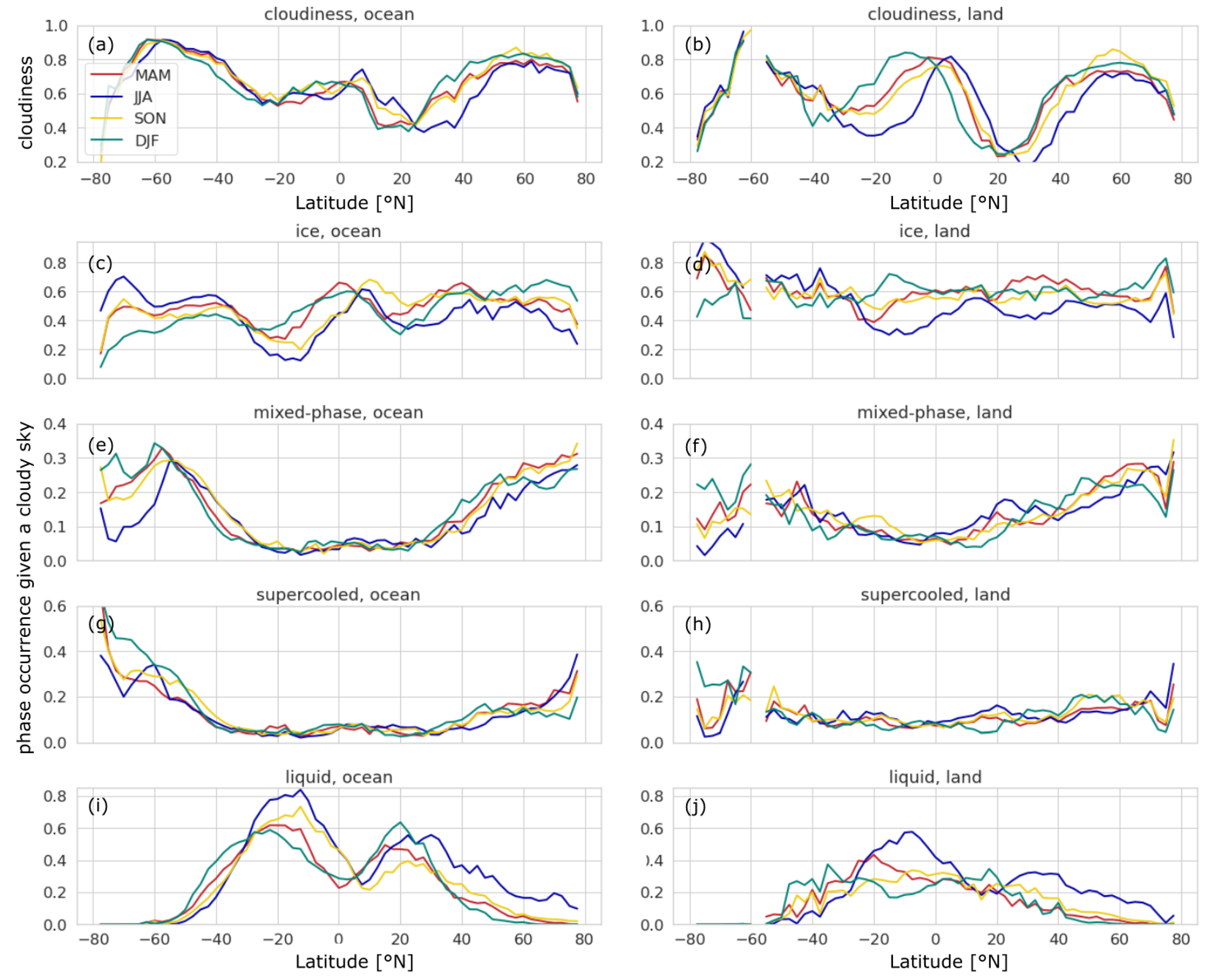
3.4. Variability with Season and Surface Type

Finally, we analyze the SEVIRI-like CTP data set in terms of seasonal variability and land-ocean differences. Figure 3 suggests that the geographical distribution of CTP is mainly controlled by latitude and surface type (ocean or land) and to a lesser degree by longitude. Therefore, in the following, the probability of phase occurrence is calculated only as a function of latitude (zonal mean), surface type, and season to obtain more robust statistics. Analog to Equation (1), incorporating season s and surface type $\mathrm{ls}$ leads to the probability of occurrence for phase q and the cloudiness

$$P\left(q\right|\mathrm{lat},\mathrm{s},\mathrm{ls})=\frac{1}{n_{\mathit{lon}}}\sum _{\mathit{lon}}P\left(q\right|\mathrm{lon},\mathrm{lat},\mathrm{s},\mathrm{ls})=\frac{1}{n_{\mathit{lon}}}\sum _{\mathit{lon}}\frac{N(q,\mathrm{lon},\mathrm{lat},\mathrm{s},\mathrm{ls})}{N\left(\mathrm{cloud},\mathrm{lon},\mathrm{lat},\mathrm{s},\mathrm{ls}\right)},$$

$$P\left(\mathrm{cloud}\right|\mathrm{lat},\mathrm{s},\mathrm{ls})=\frac{1}{n_{\mathit{lon}}}\sum _{\mathit{lon}}P\left(\mathrm{cloud}\right|\mathrm{lon},\mathrm{lat},\mathrm{s},\mathrm{ls})=\frac{1}{n_{\mathit{lon}}}\sum _{\mathit{lon}}\frac{N\left(\mathrm{cloud},\mathrm{lon},\mathrm{lat},\mathrm{s},\mathrm{ls}\right)}{N\left(\mathrm{lon},\mathrm{lat},\mathrm{s},\mathrm{ls}\right)},$$

where $n_{lon}$ is the number of longitude bins for the given ($\mathrm{lat},\mathrm{s},\mathrm{ls}$) configuration. As before, grid cells of 2.5${}^{\circ }$ are used for the longitude and latitude. Figure 6 shows the cloudiness and probability of CTP q as a function of latitude for the four seasons (DJF, MAM, JJA, SON) and two surface types (ocean, land). Because of the daylight-only mode of CloudSat, there are no data points south of 70${}^{\circ }$S for the months JJA. Due to few land masses in the southern latitudes between 40${}^{\circ }$ and 70${}^{\circ }$S, the statistics over land in these latitudes are not as robust, and the curves are therefore not as smooth as for other latitudes. The gap in the probability curves over land corresponds to latitudes where less than a minimum of 200 data points (SEVIRI-like CTPs for a given phase) are available.

In general, cloudy conditions are more frequent over the ocean than over land: mean cloudiness is about 68% over the ocean and 55% over land. This is true for most latitudes, as shown in Figure 6a,b. The only exception to this is the ITCZ because of stronger convective activity over land than over the ocean. The partitioning into CTPs, $P\left(q\right|\mathrm{lat},\mathrm{s},\mathrm{ls})$, shows ocean–land differences as well. Particularly large differences can be observed for LQ cloud tops, which in some regions in low latitudes are twice as likely to occur over the ocean than over land (26% of cloudy data points over the ocean and 16% over land). In contrast, IC cloud tops are more common over land (56%) than ocean (46%). Compared to LQ and IC cloud tops, SC and MP cloud tops show only small ocean–land differences: SC cloud tops are only slightly more common over the ocean (14%) than land (13%); MP cloud tops are equally frequent over ocean and land (14%).

Note that IC cloud tops are more frequent in the Northern than in the Southern Hemisphere: 53% of cloud tops are IC in the Northern Hemisphere, while 45% of cloud tops are IC in the Southern Hemisphere. This hemispheric difference in the occurrence of IC clouds has been reported in several studies and is attributed to the hemispheric difference in aerosol loading [72,73,74,75]. More specifically, it is attributed to the higher concentration of ice nucleating particle (INP) active mineral dust aerosol in the Northern Hemisphere, which is due to the larger land mass (especially deserts) [75]. This can also be an explanation for the hemispheric differences in SC cloud tops: for cloudy conditions, we find that 12% of the cloud tops in the Northern Hemisphere and 14% of cloud tops in the Southern Hemisphere are SC. At high latitudes, SC cloud tops are nearly twice as likely to be observed in the Southern Hemisphere, where few INPs are available for glaciation, as in the Northern Hemisphere. Huang et al. [56] also found that clouds over the Southern Ocean are more likely to be supercooled than at similar temperatures in the Northern Hemisphere, which might be connected to the availability of INPs [76].

We also observe a distinct seasonal variability in cloudiness and the CTPs, especially for IC and LQ. Over the course of a year, the maxima in the zonal mean cloudiness and the IC phase occurrence shift northwards in JJA, and then back southwards in DJF, marking high convective clouds, and therefore, the ITCZ. This shift is more pronounced over land than over the ocean, due to the higher seasonal variability of the surface temperature on land compared to the ocean. The curves for MAM and SON are mostly in between the curves for JJA and DJF. In the Southern Hemisphere, the zonal mean of cloudiness stays approximately constant during the year. However, the partitioning between the different CTPs shows a large seasonal variability. In the subtropics, LQ and IC phase occurrences have maximal differences between seasons of up to 35%, with LQ (IC) being more frequent in JJA (DJF). In the southern high latitudes (south of 60${}^{\circ }$S), the largest seasonal variabilities are observed for IC and MP phase occurrences.

In contrast to the Southern Hemisphere, cloudiness shows large seasonal variability in the northern mid and high latitudes: Cloudiness is highest in DJF and lowest in JJA. A second difference to the Southern Hemisphere is that in the Northern Hemisphere LQ cloud tops are observed also at high latitudes, occurring mainly in JJA. The higher occurrences of LQ cloud tops during JJA are partially compensated through lower probabilities of occurrence for IC and MP cloud tops. In contrast to IC, MP, and LQ cloud tops, SC cloud tops exhibit little seasonal variability in the northern high latitudes.

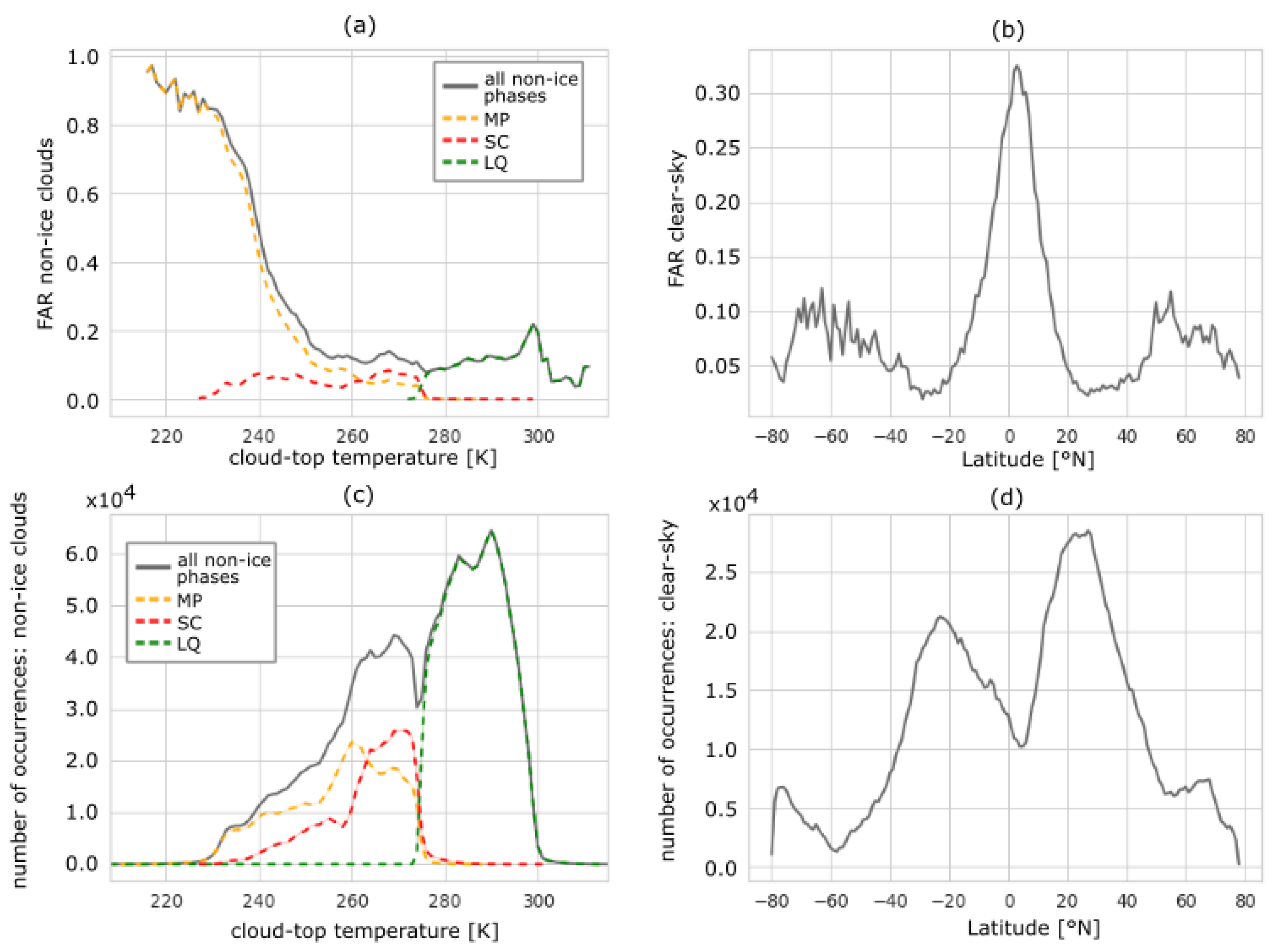
4. Evaluation of CiPS

In this section, the performance of the ice cloud detection algorithm CiPS is evaluated using the SEVIRI-like CTP derived from DARDAR as a reference (see Section 2.2). The output of the CiPS ice detection is either “ice” or “non-ice” for every pixel. Hence, in order to compare the SEVIRI-like CTP to CiPS, we summarize the categories clear-sky, LQ, SC, and MP of the SEVIRI-like data set to the category “non-ice”, while the IC CTP category of the SEVIRI-like data set is comparable to the CiPS “ice” category. For the evaluation of CiPS, we use one year (2013) of the SEVIRI-like data set and compare its “ice” and “non-ice” values pixel by pixel with the results of CiPS at the same latitude, longitude, and time. The number of data points in which both data sets agree (i.e., either “ice” or “non-ice” in both data sets) or disagree (i.e., “ice” in one data set and “non-ice” in the other data set) are counted. The results of this comparison are displayed in

Table 1. Percentages of pixels classified as ice or non-ice by CiPS with respect to the SEVIRI-like classification.

	DARDAR: Ice	DARDAR: Non-Ice
CiPS: ice	77.1%	11.6%
CiPS: non-ice	22.9%	88.4%

. It shows the percentage of pixels classified by CiPS as either ice or non-ice pixels with respect to a fixed category of the SEVIRI-like data set. For the SEVIRI-like data set, all ice cloud pixels observed during the year 2013 amount to about 1.9 × 10${}^6$ data points, while non-ice pixels amount to about 4.2 × 10${}^6$ data points. Of these pixels classified as ice in the SEVIRI-like data set, CiPS detects 77.1% as ice as well, i.e., its probability of detection (POD) amounts to this value. The ice clouds that remain undetected by CiPS are mainly optically thin clouds with optical thickness < 1, which are known to be difficult to detect with passive methods [50]. As mentioned in Section 2.2, CiPS was trained to detect ice crystals with CAL_LID_L2, which distinguishes “only” between ice clouds, liquid water clouds, and “undetermined”. Consequently, in the previous characterization of Strandgren et al. [50], it was not possible to test how CiPS performs for MP clouds, particularly whether CiPS is sensitive to ice crystals present in MP clouds. Using the collocated data set of SEVIRI-like CTP and CiPS, this can now be examined. We find that CiPS categorizes only 22% of MP clouds as ice. The rest of the MP clouds, i.e., 78%, are categorized as non-ice. Thus, the detection of cloud ice by CiPS is mostly limited to pure ice clouds.

The false alarm rate, FAR, (i.e., the fraction of SEVIRI-like non-ice pixels which are classified as ice by CiPS) is 11.6%. Of these pixels falsely classified as ice by CiPS, 32% are clear-sky according to the SEVIRI-like data set, and the rest are cloudy with 28% LQ, 27% MP, and 13% SC cloud tops. Since the fraction of misclassified MP clouds is overproportionally large compared to the occurrence of this phase, we can conclude that phase discrimination between IC and MP clouds is a particular challenge for CiPS. In order to understand the FAR of CiPS better, we examine its dependencies. We find that the FAR of CiPS for clear-sky (i.e., pixels classified as clear-sky in the SEVIRI-like data set and as ice by CiPS) depends mainly on the latitude, while the FAR of CiPS for non-ice cloudy pixels (i.e., pixels classified as LQ, SC or MP in the SEVIRI-like data set and as ice by CiPS) depends mainly on CTT. Figure 7a,b shows these dependencies of the FAR of CiPS for non-ice cloudy and clear-sky pixels. The panels below (Figure 7c,d) show the number of occurrences of the non-ice cloudy and clear-sky pixels to indicate the frequency at which the respective FARs occur. The FAR for non-ice cloudy pixels as a function of CTT (see Figure 7a) is nearly constant (and small, around 0.1) for clouds with CTT ≥ 250 K and increases strongly below this temperature for MP cloud tops. Interestingly, SC clouds are only responsible for a very small amount of false alarms, in contrast to the findings of Strandgren et al. [50] (see Section 2.2). The FAR for clear-sky conditions as a function of latitude (see Figure 7b) shows that most false alarms are found in the ITCZ with high surface temperatures, which is a known weakness of CiPS [49] (see also Section 2.2). In the evaluation of CiPS Strandgren et al. [49,50] (as mentioned in Section 2.2), similar results were found for the POD (70%) as in this study, but lower values for the FAR (4%). Since CiPS was trained with CAL_LID_L2, a better agreement is to be expected. There are several factors that can account for these differences in FAR. One factor is differences in phase partitioning. According to the definition of the CTP, pixels at SEVIRI resolution composed of DARDAR gates that are partly ice and partly other phases (MP or SC) are classified as MP. Some such pixels composed mainly of ice with a small liquid fraction could fall into the ice category of the coarser CAL_LID_L2 product. This would lead to an increase in the FAR of CiPS. In addition, the two products DARDAR and CAL_LID_L2 use different algorithms to determine the cloud thermodynamic phase which could lead to inherent differences in the phase partitioning of the two products, increasing the FAR of CiPS. Furthermore, both products use different cloud masks: DARDAR uses the CALIPSO Vertical Feature Mask only to filter out aerosols and otherwise CALIOP backscatter directly, while the product used to train CiPS is version V3-01 of CAL_LID_L2_05kmC [61]. A third difference between the evaluation of CiPS in this study and the previous evaluation of Strandgren et al. [50] is that the training and previous evaluation of CiPS was performed with MSG2 data, while we use MSG3 data in this study. The channels of the two different satellites are not completely identical, and CiPS is expected to perform better on MSG2. Since the two evaluations cover different time periods, there is also the possibility that differences in clouds in the two time periods led to the differences in FAR.

5. Discussion and Conclusions

Since phase partitioning is still an open question in climate modeling and has important implications for various cloud-related subjects (precipitation, cloud lifetime, cloud albedo, ...) the goal of this paper is to understand the importance of the four different phases (IC, MP, SC, and LQ) in terms of their frequency of occurrence from the geostationary perspective. Since MP and SC clouds are most prevalent at high latitudes which are difficult to see with a geostationary satellite, it is not a priori clear how many MP and SC cloud tops can be observed with SEVIRI. To our knowledge, no information about the occurrence of such phases is available at the SEVIRI pixel level.

To gain new insights about these questions, we use the lidar/radar remote sensing product DARDAR-MASK to deduce a cloud top phase (CTP) for the geostationary passive sensor SEVIRI aboard Meteosat Second Generation. This SEVIRI-like CTP is then used to test the influence of the resolution on CTP measurements and to study the geographic and seasonal distribution of CTPs from a geostationary passive satellite perspective as well as to evaluate the ice cloud detection algorithm for SEVIRI called CiPS.

To deduce the SEVIRI-like CTP from DARDAR measurements, we impose a (simplified) penetration depth of SEVIRI by only considering DARDAR values up to 240 m below cloud top and aggregating the DARDAR results to the spatial resolution of SEVIRI. This results in a CTP in SEVIRI resolution with four different thermodynamic “phases”: ice (IC), mixed-phase (MP), supercooled (SC), and warm liquid (LQ). Testing this derived SEVIRI-like CTP against CTT shows that aggregating the DARDAR cloud phase to the lower SEVIRI resolution preserves physical relationships. Although the data set was derived for the viewing geometry and resolution of SEVIRI, it can be easily extended to other geostationary satellites, provided sufficient data are available for collocation. In this sense, it will not be possible to derive a similar data set for the Flexible Combined Imager (FCI) aboard the follow-on satellite of MSG (Meteosat Third Generation—MTG, launched on 13 December 2022 [77]), since the spaceborne active instruments from the A-Train will no longer be available in 2023. Future observations from the EarthCARE satellite [78] will be needed.

We use the aggregated SEVIRI-like CTP to test the effects of the resolution on the cloud phase measurements by comparing the CTP at SEVIRI resolution with a corresponding CTP at DARDAR resolution. Even though the general patterns of CTP are similar in both resolutions, we find that the resolution has a significant effect on the occurrence of the CTPs and their geographic distribution. The largest changes due to resolution are found for MP cloud tops, which occur significantly more often at the lower SEVIRI resolution (14% on average) than at the higher DARDAR resolution (9% on average). In contrast, the probability of measuring SC or IC cloud tops decreases for the lower SEVIRI resolution. We also find effects due to partly cloud-covered pixels and edges between clouds, which mainly influence the occurrence of LQ and IC cloud tops in the SEVIRI-like data set. These results help to assess how representative geostationary measurements of CTP are compared to measurements from polar orbit satellites and to interpret them in the correct way.

From the SEVIRI-like data set, we find that all four different CTPs are found in significant amounts on the Meteosat disk: In SEVIRI resolution, 65.0% of data points are cloudy, consisting of 49% IC, 14% MP, 13% SC, and 24% LQ cloud tops. For CTTs above 246 K, MP, or SC clouds are predominant, while IC clouds become dominant for lower temperatures. An analysis of the CTH distribution for different latitude regions reveals that the different CTPs have characteristic height regimes, however, with large overlaps, especially between MP and SC clouds. In the tropics, the CTH regimes of MP/SC and LQ are clearly separated, with LQ at lower heights, while the CTH regimes of LQ, SC, and MP strongly overlap in the mid- and high-latitudes. Even though the altitude regime of IC extends much higher than the other phases, it also has overlap with those of the other CTPs. Interestingly, MP and SC cloud tops have a very similar average CTH value and vertical distribution in the tropics with predominantly convective systems but show differences in CTH at mid and high latitudes where stratiform clouds dominate for MP and SC. For a retrieval with SEVIRI, the observed differences in the characteristic height regimes of the CTPs can serve as a starting point for the distinction between phases. However, due to the large overlap of height regimes of the CTPs, a distinction can not be made on the basis of CTH (or the correlated CTT) alone.

The amount of cloudiness exhibits a distinct seasonal cycle, particularly over land where it follows the seasonal progression of the ITCZ. The probability of IC also varies in a similar manner to the ITCZ. LQ shows a clear seasonal cycle affected by the shift of the ITCZ as well, especially in the subtropics. On the contrary, MP and SC show less seasonal variability, with the largest seasonal fluctuations being observed in Antarctica. There, the probability of MP and SC clouds is at its minimum during JJA and at its peak during DJF, with a difference of up to 20% between seasons.

As an application of the SEVIRI-like CTP data set, we evaluate CiPS, a state-of-the-art AI-based ice cloud detection algorithm for SEVIRI. We find that CiPS performs well with a probability of detection of 77.1% and a false alarm rate of 11.6%. False alarms occur mainly for cold MP cloud tops and for clear-sky conditions in the ITCZ. Even though MP cloud tops have the highest FAR in cloudy conditions, CiPS classifies overall only 22% of MP clouds as ice. The rest of the MP cloud tops are classified as non-ice, which means that CiPS is not sensitive to the ice particles contained in MP clouds. This suggests that new methods are needed to detect MP cloud tops from SEVIRI data.

Finally, our results stress the need for phase determination algorithms for SEVIRI that are able to discriminate among all these phase conditions and can be used to develop or test phase retrievals. This study shows that all thermodynamic phases occur frequently over the Meteosat disk. Therefore, a retrieval for all thermodynamic phases for SEVIRI would provide an important contribution to better understand phase partitioning and enable us to investigate the micro- and macrophysics of MP, SC, and LQ clouds. This would be a valuable addition to the CiPS algorithm, which is “only” suited to detect fully glaciated clouds. In addition, the high temporal resolution of SEVIRI would also allow us to study the evolution of clouds and their top phase, thus extending the value of the DARDAR-MASK product to places and times where no data from CloudSat and CALIPSO are available because of their sun-synchronous polar orbits. In this context, the SEVIRI-like CTP could also serve as a “ground truth” to develop and test new phase retrievals for SEVIRI. There are nearly 20 years of data from the SEVIRI instrument (the Meteosat Second Generation satellites have been in operation since 2004) waiting to be evaluated with respect to CTP.

References

1. Boucher, O.; Randall, D.; Artaxo, P.; Bretherton, C.; Feingold, G.; Forster, P.; Kerminen, V.M.; Kondo, Y.; Liao, H.; Lohmann, U.; et al. Clouds and Aerosols. In Climate Change 2013: The Physical Science Basis. Contribution of Working Group I to the Fifth Assessment Report of the Intergovernmental Panel on Climate Change; Stocker, T.F., Qin, D., Plattner, G.-K., Tignor, M., Allen, S.K., Boschung, J., Nauels, A., Xia, Y., Bex, V., Midgley, P.M., Eds.; Cambridge University Press: Cambridge, UK; New York, NY, USA, 2013; pp. 571–658. [Google Scholar] [CrossRef]
2. Forster, P.; Storelvmo, T.; Armour, K.; Collins, W.; Dufresne, J.L.; Frame, D.; Lunt, D.; Mauritsen, T.; Palmer, M.; Watanabe, M.; et al. The Earth’s Energy Budget, Climate Feedbacks, and Climate Sensitivity. In Climate Change 2021: The Physical Science Basis. Contribution of Working Group I to the Sixth Assessment Report of the Intergovernmental Panel on Climate Change; Masson-Delmotte, V., Zhai, P., Pirani, A., Connors, S.L., Péan, C., Berger, S., Caud, N., Chen, Y., Goldfarb, L., Gomis, M.I., et al., Eds.; Cambridge University Press: Cambridge, UK; New York, NY, USA, 2021; pp. 923–1054. [Google Scholar] [CrossRef]
3. Ehrlich, A.; Bierwirth, E.; Wendisch, M.; Gayet, J.F.; Mioche, G.; Lampert, A.; Heintzenberg, J. Cloud phase identification of Arctic boundary-layer clouds from airborne spectral reflection measurements: Test of three approaches. Atmos. Chem. Phys. 2008, 8, 7493–7505. [Google Scholar] [CrossRef] [Green Version]
4. Tan, I.; Storelvmo, T.; Zelinka, M.D. Observational constraints on mixed-phase clouds imply higher climate sensitivity. Science 2016, 352, 224–227. [Google Scholar] [CrossRef] [PubMed] [Green Version]
5. Thompson, D.R.; Kahn, B.H.; Green, R.O.; Chien, S.A.; Middleton, E.M.; Tran, D.Q. Global spectroscopic survey of cloud thermodynamic phase at high spatial resolution, 2005–2015. Atmos. Meas. Tech. 2018, 11, 1019–1030. [Google Scholar] [CrossRef] [Green Version]
6. McCoy, D.T.; Hartmann, D.L.; Zelinka, M.D.; Ceppi, P.; Grosvenor, D.P. Mixed-phase cloud physics and Southern Ocean cloud feedback in climate models. J. Geophys. Res. Atmos. 2015, 120, 9539–9554. [Google Scholar] [CrossRef]
7. Choi, Y.S.; Ho, C.H.; Park, C.E.; Storelvmo, T.; Tan, I. Influence of cloud phase composition on climate feedbacks. J. Geophys. Res. Atmos. 2014, 119, 3687–3700. [Google Scholar] [CrossRef]
8. Komurcu, M.; Storelvmo, T.; Tan, I.; Lohmann, U.; Yun, Y.; Penner, J.E.; Wang, Y.; Liu, X.; Takemura, T. Intercomparison of the cloud water phase among global climate models. J. Geophys. Res. Atmos. 2014, 119, 3372–3400. [Google Scholar] [CrossRef] [Green Version]
9. Mioche, G.; Jourdan, O.; Ceccaldi, M.; Delanoë, J. Variability of mixed-phase clouds in the Arctic with a focus on the Svalbard region: A study based on spaceborne active remote sensing. Atmos. Chem. Phys. 2015, 15, 2445–2461. [Google Scholar] [CrossRef] [Green Version]
10. Matus, A.V.; L’Ecuyer, T.S. The role of cloud phase in Earths radiation budget. J. Geophys. Res. Atmos. 2017, 122, 2559–2578. [Google Scholar] [CrossRef]
11. Ricaud, P.; Guasta, M.D.; Lupi, A.; Roehrig, R.; Bazile, E.; Durand, P.; Attié, J.L.; Nicosia, A.; Grigioni, P. Supercooled liquid water clouds observed over Dome C, Antarctica: Temperature sensitivity and surface radiation impact. Atmos. Chem. Phys. Discuss. 2022. [Google Scholar] [CrossRef]
12. Cheng, A.; Xu, K.M.; Hu, Y.; Kato, S. Impact of a cloud thermodynamic phase parameterization based on CALIPSO observations on climate simulation. J. Geophys. Res. Atmos. 2012, 117, D09103. [Google Scholar] [CrossRef]
13. Cesana, G.; Waliser, D.E.; Jiang, X.; Li, J.L.F. Multimodel evaluation of cloud phase transition using satellite and reanalysis data. J. Geophys. Res. Atmos. 2015, 120, 7871–7892. [Google Scholar] [CrossRef]
14. Zhang, D.; Liu, D.; Luo, T.; Wang, Z.; Yin, Y. Aerosol impacts on cloud thermodynamic phase change over East Asia observed with CALIPSO and CloudSat measurements. J. Geophys. Res. Atmos. 2015, 120, 1490–1501. [Google Scholar] [CrossRef]
15. Braga, R.C.; Rosenfeld, D.; Weigel, R.; Jurkat, T.; Andreae, M.O.; Wendisch, M.; Pöschl, U.; Voigt, C.; Mahnke, C.; Borrmann, S.; et al. Further evidence for CCN aerosol concentrations determining the height of warm rain and ice initiation in convective clouds over the Amazon basin. Atmos. Chem. Phys. 2017, 17, 14433–14456. [Google Scholar] [CrossRef] [Green Version]
16. Coopman, Q.; Hoose, C.; Stengel, M. Analyzing the Thermodynamic Phase Partitioning of Mixed Phase Clouds Over the Southern Ocean Using Passive Satellite Observations. Geophys. Res. Lett. 2021, 48, e2021GL093225. [Google Scholar] [CrossRef]
17. Atkinson, J.D.; Murray, B.J.; Woodhouse, M.T.; Whale, T.F.; Baustian, K.J.; Carslaw, K.S.; Dobbie, S.; O’Sullivan, D.; Malkin, T.L. The importance of feldspar for ice nucleation by mineral dust in mixed-phase clouds. Nature 2013, 498, 355–358. [Google Scholar] [CrossRef] [PubMed] [Green Version]
18. Prenni, A.J.; Harrington, J.Y.; Tjernström, M.; DeMott, P.J.; Avramov, A.; Long, C.N.; Kreidenweis, S.M.; Olsson, P.Q.; Verlinde, J. Can Ice-Nucleating Aerosols Affect Arctic Seasonal Climate? Bull. Am. Meteorol. Soc. 2007, 88, 541–550. [Google Scholar] [CrossRef] [Green Version]
19. Morrison, H.; Zuidema, P.; Ackerman, A.S.; Avramov, A.; de Boer, G.; Fan, J.; Fridlind, A.M.; Hashino, T.; Harrington, J.Y.; Luo, Y.; et al. Intercomparison of cloud model simulations of Arctic mixed-phase boundary layer clouds observed during SHEBA/FIRE-ACE. J. Adv. Model. Earth Syst. 2011, 3, 66. [Google Scholar] [CrossRef]
20. Gregory, D.; Morris, D. The sensitivity of climate simulations to the specification of mixed phase clouds. Clim. Dyn. 1996, 12, 641–651. [Google Scholar] [CrossRef]
21. Doutriaux-Boucher, M.; Quaas, J. Evaluation of cloud thermodynamic phase parametrizations in the LMDZ GCM by using POLDER satellite data. Geophys. Res. Lett. 2004, 31, L06126. [Google Scholar] [CrossRef] [Green Version]
22. Cesana, G.; Kay, J.E.; Chepfer, H.; English, J.M.; Boer, G. Ubiquitous low-level liquid-containing Arctic clouds: New observations and climate model constraints from CALIPSO-GOCCP. Geophys. Res. Lett. 2012, 39, 53385. [Google Scholar] [CrossRef] [Green Version]
23. Stubenrauch, C.J.; Rossow, W.B.; Kinne, S.; Ackerman, S.; Cesana, G.; Chepfer, H.; Girolamo, L.D.; Getzewich, B.; Guignard, A.; Heidinger, A.; et al. Assessment of Global Cloud Datasets from Satellites: Project and Database Initiated by the GEWEX Radiation Panel. Bull. Am. Meteorol. Soc. 2013, 94, 1031–1049. [Google Scholar] [CrossRef]
24. Stubenrauch, C.J.; Feofilov, A.G.; Protopapadaki, S.E.; Armante, R. Cloud climatologies from the infrared sounders AIRS and IASI: Strengths and applications. Atmos. Chem. Phys. 2017, 17, 13625–13644. [Google Scholar] [CrossRef] [Green Version]
25. Li, W.; Zhang, F.; Lin, H.; Chen, X.; Li, J.; Han, W. Cloud Detection and Classification Algorithms for Himawari-8 Imager Measurements Based on Deep Learning. IEEE Trans. Geosci. Remote Sens. 2022, 60, 1–17. [Google Scholar] [CrossRef]
26. Zhou, G.; Wang, J.; Yin, Y.; Hu, X.; Letu, H.; Sohn, B.J.; Yung, Y.L.; Liu, C. Detecting Supercooled Water Clouds Using Passive Radiometer Measurements. Geophys. Res. Lett. 2022, 49, e2021GL096111. [Google Scholar] [CrossRef]
27. Hu, Y.; Winker, D.; Vaughan, M.; Lin, B.; Omar, A.; Trepte, C.; Flittner, D.; Yang, P.; Nasiri, S.L.; Baum, B.; et al. CALIPSO/CALIOP Cloud Phase Discrimination Algorithm. J. Atmos. Ocean. Technol. 2009, 26, 2293–2309. [Google Scholar] [CrossRef] [Green Version]
28. Hu, Y.; Rodier, S.; man Xu, K.; Sun, W.; Huang, J.; Lin, B.; Zhai, P.; Josset, D. Occurrence, liquid water content, and fraction of supercooled water clouds from combined CALIOP/IIR/MODIS measurements. J. Geophys. Res. 2010, 115, 2384. [Google Scholar] [CrossRef]
29. Luke, E.P.; Kollias, P.; Shupe, M.D. Detection of supercooled liquid in mixed-phase clouds using radar Doppler spectra. J. Geophys. Res. 2010, 115, 2884. [Google Scholar] [CrossRef] [Green Version]
30. Zhang, D.; Wang, Z.; Liu, D. A global view of midlevel liquid-layer topped stratiform cloud distribution and phase partition from CALIPSO and CloudSat measurements. J. Geophys. Res. 2010, 115, 2143. [Google Scholar] [CrossRef] [Green Version]
31. Cesana, G.; Storelvmo, T. Improving climate projections by understanding how cloud phase affects radiation. J. Geophys. Res. Atmos. 2017, 122, 4594–4599. [Google Scholar] [CrossRef]
32. Bruno, O.; Hoose, C.; Storelvmo, T.; Coopman, Q.; Stengel, M. Exploring the Cloud Top Phase Partitioning in Different Cloud Types Using Active and Passive Satellite Sensors. Geophys. Res. Lett. 2021, 48, 89863. [Google Scholar] [CrossRef]
33. Korolev, A.; McFarquhar, G.; Field, P.R.; Franklin, C.; Lawson, P.; Wang, Z.; Williams, E.; Abel, S.J.; Axisa, D.; Borrmann, S.; et al. Mixed-Phase Clouds: Progress and Challenges. Meteorol. Monogr. 2017, 58, 51–550. [Google Scholar] [CrossRef]
34. Wang, Z. Level 2 Combined Radar and Lidar Cloud Scenario Classification Product Process Description and Interface Control Document; Report 22; Jet Propulsion Laboratory: Pasadena, CA, USA, 2012. [Google Scholar]
35. Delanoë, J.; Hogan, R.J. A variational scheme for retrieving ice cloud properties from combined radar, lidar, and infrared radiometer. J. Geophys. Res. 2008, 113, D07204. [Google Scholar] [CrossRef] [Green Version]
36. Ewald, F.; Groß, S.; Wirth, M.; Delanoë, J.; Fox, S.; Mayer, B. Why we need radar, lidar, and solar radiance observations to constrain ice cloud microphysics. Atmos. Meas. Tech. 2021, 14, 5029–5047. [Google Scholar] [CrossRef]
37. Listowski, C.; Delanoë, J.; Kirchgaessner, A.; Lachlan-Cope, T.; King, J. Antarctic clouds, supercooled liquid water and mixed phase, investigated with DARDAR: Geographical and seasonal variations. Atmos. Chem. Phys. 2019, 19, 6771–6808. [Google Scholar] [CrossRef] [Green Version]
38. Okamoto, H.; Sato, K.; Hagihara, Y. Global analysis of ice microphysics from CloudSat and CALIPSO: Incorporation of specular reflection in lidar signals. J. Geophys. Res. 2010, 115, 13383. [Google Scholar] [CrossRef]
39. Zaremba, T.J.; Rauber, R.M.; McFarquhar, G.M.; Hayman, M.; Finlon, J.A.; Stechman, D.M. Phase Characterization of Cold Sector Southern Ocean Cloud Tops: Results From SOCRATES. J. Geophys. Res. Atmos. 2020, 125, 33673. [Google Scholar] [CrossRef]
40. Rauber, R.M.; Tokay, A. An Explanation for the Existence of Supercooled Water at the Top of Cold Clouds. J. Atmos. Sci. 1991, 48, 1005–1023. [Google Scholar] [CrossRef]
41. Khain, A.; Pinsky, M.; Korolev, A. Combined Effect of the Wegener–Bergeron–Findeisen Mechanism and Large Eddies on Microphysics of Mixed-Phase Stratiform Clouds. J. Atmos. Sci. 2022, 79, 383–407. [Google Scholar] [CrossRef]
42. Baum, B.A.; Menzel, W.P.; Frey, R.A.; Tobin, D.C.; Holz, R.E.; Ackerman, S.A.; Heidinger, A.K.; Yang, P. MODIS Cloud-Top Property Refinements for Collection 6. J. Appl. Meteorol. Climatol. 2012, 51, 1145–1163. [Google Scholar] [CrossRef]
43. Key, J.R.; Intrieri, J.M. Cloud Particle Phase Determination with the AVHRR. J. Appl. Meteorol. 2000, 39, 1797–1804. [Google Scholar] [CrossRef]
44. Platnick, S.; Meyer, K.G.; King, M.D.; Wind, G.; Amarasinghe, N.; Marchant, B.; Arnold, G.T.; Zhang, Z.; Hubanks, P.A.; Holz, R.E.; et al. The MODIS Cloud Optical and Microphysical Products: Collection 6 Updates and Examples From Terra and Aqua. IEEE Trans. Geosci. Remote Sens. 2017, 55, 502–525. [Google Scholar] [CrossRef] [Green Version]
45. Bessho, K.; Date, K.; Hayashi, M.; Ikeda, A.; Imai, T.; Inoue, H.; Kumagai, Y.; Miyakawa, T.; Murata, H.; Ohno, T.; et al. An Introduction to Himawari-8/9-Japan’s New-Generation Geostationary Meteorological Satellites. J. Meteorol. Soc. Japan. Ser. II 2016, 94, 151–183. [Google Scholar] [CrossRef] [Green Version]
46. Benas, N.; Finkensieper, S.; Stengel, M.; van Zadelhoff, G.J.; Hanschmann, T.; Hollmann, R.; Meirink, J.F. The MSG-SEVIRI-based cloud property data record CLAAS-2. Earth Syst. Sci. Data 2017, 9, 415–434. [Google Scholar] [CrossRef] [Green Version]
47. Pavolonis, M. GOES-R Advanced Baseline Imager (ABI) Algorithm Theoretical Basis Document For Cloud Type and Cloud Phase. 2010. Available online: https://www.star.nesdis.noaa.gov/smcd/spb/aq/AerosolWatch/docs/GOES-R_ABI_AOD_ATBD_V4.2_20180214.pdf (accessed on 12 January 2023).
48. Wang, Z.; Letu, H.; Shang, H.; Zhao, C.; Li, J.; Ma, R. A Supercooled Water Cloud Detection Algorithm Using Himawari-8 Satellite Measurements. J. Geophys. Res. Atmos. 2019, 124, 2724–2738. [Google Scholar] [CrossRef]
49. Strandgren, J.; Bugliaro, L.; Sehnke, F.; Schröder, L. Cirrus cloud retrieval with MSG/SEVIRI using artificial neural networks. Atmos. Meas. Tech. 2017, 10, 3547–3573. [Google Scholar] [CrossRef] [Green Version]
50. Strandgren, J.; Fricker, J.; Bugliaro, L. Characterisation of the artificial neural network CiPS for cirrus cloud remote sensing with MSG/SEVIRI. Atmos. Meas. Tech. 2017, 10, 4317–4339. [Google Scholar] [CrossRef] [Green Version]
51. Baum, B.A.; Spinhirne, J.D. Remote sensing of cloud properties using MODIS airborne simulator imagery during SUCCESS: 3. Cloud Overlap. J. Geophys. Res. Atmos. 2000, 105, 11793–11804. [Google Scholar] [CrossRef]
52. Cesana, G.; Chepfer, H. Evaluation of the cloud thermodynamic phase in a climate model using CALIPSO-GOCCP. J. Geophys. Res. Atmos. 2013, 118, 7922–7937. [Google Scholar] [CrossRef]
53. Delanoë, J.; Hogan, R.J. Combined CloudSat-CALIPSO-MODIS retrievals of the properties of ice clouds. J. Geophys. Res. 2010, 115, 12346. [Google Scholar] [CrossRef] [Green Version]
54. Ceccaldi, M.; Delanoë, J.; Hogan, R.J.; Pounder, N.L.; Protat, A.; Pelon, J. From CloudSat-CALIPSO to EarthCare: Evolution of the DARDAR cloud classification and its comparison to airborne radar-lidar observations. J. Geophys. Res. Atmos. 2013, 118, 7962–7981. [Google Scholar] [CrossRef]
55. Delanoë, J.; Protat, A.; Jourdan, O.; Pelon, J.; Papazzoni, M.; Dupuy, R.; Gayet, J.F.; Jouan, C. Comparison of Airborne In Situ, Airborne Radar–Lidar, and Spaceborne Radar–Lidar Retrievals of Polar Ice Cloud Properties Sampled during the POLARCAT Campaign. J. Atmos. Ocean. Technol. 2013, 30, 57–73. [Google Scholar] [CrossRef]
56. Huang, Y.; Siems, S.T.; Manton, M.J.; Protat, A.; Delanoë, J. A study on the low-altitude clouds over the Southern Ocean using the DARDAR-MASK. J. Geophys. Res. Atmos. 2012, 117, 17800. [Google Scholar] [CrossRef]
57. Huang, Y.; Protat, A.; Siems, S.T.; Manton, M.J. A-Train Observations of Maritime Midlatitude Storm-Track Cloud Systems: Comparing the Southern Ocean against the North Atlantic. J. Clim. 2015, 28, 1920–1939. [Google Scholar] [CrossRef]
58. Benedetti, A. CloudSat AN-ECMWF Ancillary Data Interface Control Document, Technical Document; CloudSat Data Processing Center: Fort Collins, CO, USA, 2005. [Google Scholar]
59. Hogan, R.J.; Francis, P.N.; Flentje, H.; Illingworth, A.J.; Quante, M.; Pelon, J. Characteristics of mixed-phase clouds. I: Lidar, radar and aircraft observations from CLARE’98. Q. J. R. Meteorol. Soc. 2003, 129, 2089–2116. [Google Scholar] [CrossRef] [Green Version]
60. Westbrook, C.D.; Illingworth, A.J. The formation of ice in a long-lived supercooled layer cloud. Q. J. R. Meteorol. Soc. 2013, 139, 2209–2221. [Google Scholar] [CrossRef] [Green Version]
61. Winker, D. CALIPSO LID_L2_05kmALay-Prov HDF File-Version 3.30; Atmospheric Science Data Center: Washington, DC, USA, 2013. [Google Scholar] [CrossRef]
62. Platnick, S. Vertical photon transport in cloud remote sensing problems. J. Geophys. Res. Atmos. 2000, 105, 22919–22935. [Google Scholar] [CrossRef] [Green Version]
63. Korolev, A.; Milbrandt, J. How Are Mixed-Phase Clouds Mixed? Geophys. Res. Lett. 2022, 49, 99578. [Google Scholar] [CrossRef]
64. Hersbach, H.; Bell, B.; Berrisford, P.; Hirahara, S.; Horányi, A.; Muñoz-Sabater, J.; Nicolas, J.; Peubey, C.; Radu, R.; Schepers, D.; et al. The ERA5 global reanalysis. Q. J. R. Meteorol. Soc. 2020, 146, 1999–2049. [Google Scholar] [CrossRef]
65. Verlinden, K.L.; Thompson, D.W.J.; Stephens, G.L. The Three-Dimensional Distribution of Clouds over the Southern Hemisphere High Latitudes. J. Clim. 2011, 24, 5799–5811. [Google Scholar] [CrossRef]
66. Bromwich, D.H.; Nicolas, J.P.; Hines, K.M.; Kay, J.E.; Key, E.L.; Lazzara, M.A.; Lubin, D.; McFarquhar, G.M.; Gorodetskaya, I.V.; Grosvenor, D.P.; et al. Tropospheric clouds in Antarctica. Rev. Geophys. 2012, 50, 363. [Google Scholar] [CrossRef] [Green Version]
67. Adhikari, L.; Wang, Z.; Deng, M. Seasonal variations of Antarctic clouds observed by CloudSat and CALIPSO satellites. J. Geophys. Res. Atmos. 2012, 117, 16719. [Google Scholar] [CrossRef] [Green Version]
68. McFarquhar, G.M. Observations of Clouds, Aerosols, Precipitation, and Surface Radiation over the Southern Ocean: An Overview of CAPRICORN, MARCUS, MICRE, and SOCRATES. Bull. Am. Meteorol. Soc. 2021, 102, E894–E928. [Google Scholar] [CrossRef]
69. Schima, J.; McFarquhar, G.; Romatschke, U.; Vivekanandan, J.; D’Alessandro, J.; Haggerty, J.; Wolff, C.; Schaefer, E.; Järvinen, E.; Schnaiter, M. Characterization of Southern Ocean Boundary Layer Clouds Using Airborne Radar, Lidar, and In Situ Cloud Data: Results From SOCRATES. J. Geophys. Res. Atmos. 2022, 127, e2022JD037277. [Google Scholar] [CrossRef]
70. Truong, S.C.H.; Huang, Y.; Siems, S.T.; Manton, M.J.; Lang, F. Biases in the thermodynamic structure over the Southern Ocean in ERA5 and their radiative implications. Int. J. Climatol. 2022, 42, 7685–7702. [Google Scholar] [CrossRef]
71. Hogan, R.J.; O’Connor, E.J. Facilitating Cloud Radarand Lidar Algorithms: The Cloudnet InstrumentSynergy/Target Categorization Product. 2006. Available online: www.cloud-net.org/data/products/categorize.html (accessed on 20 March 2023).
72. Tan, I.; Storelvmo, T.; Choi, Y.S. Spaceborne lidar observations of the ice-nucleating potential of dust, polluted dust, and smoke aerosols in mixed-phase clouds. J. Geophys. Res. Atmos. 2014, 119, 6653–6665. [Google Scholar] [CrossRef]
73. Zhang, D.; Wang, Z.; Kollias, P.; Vogelmann, A.M.; Yang, K.; Luo, T. Ice particle production in mid-level stratiform mixed-phase clouds observed with collocated A-Train measurements. Atmos. Chem. Phys. 2018, 18, 4317–4327. [Google Scholar] [CrossRef] [Green Version]
74. Li, J.; Lv, Q.; Zhang, M.; Wang, T.; Kawamoto, K.; Chen, S.; Zhang, B. Effects of atmospheric dynamics and aerosols on the fraction of supercooled water clouds. Atmos. Chem. Phys. 2017, 17, 1847–1863. [Google Scholar] [CrossRef] [Green Version]
75. Villanueva, D.; Senf, F.; Tegen, I. Hemispheric and seasonal contrast in cloud thermodynamic phase from A-Train spaceborne instruments. J. Geophys. Res. Atmos. 2021, 126, e2020JD034322. [Google Scholar] [CrossRef]
76. Twohy, C.H.; DeMott, P.J.; Russell, L.M.; Toohey, D.W.; Rainwater, B.; Geiss, R.; Sanchez, K.J.; Lewis, S.; Roberts, G.C.; Humphries, R.S.; et al. Cloud-Nucleating Particles Over the Southern Ocean in a Changing Climate. Earth’s Future 2021, 9, 1673. [Google Scholar] [CrossRef]
77. Durand, Y.; Hallibert, P.; Wilson, M.; Lekouara, M.; Grabarnik, S.; Aminou, D.; Blythe, P.; Napierala, B.; Canaud, J.L.; Pigouche, O.; et al. The Flexible Combined Imager Onboard MTG: From Design to Calibration. Proc. SPIE 2015, 9639, 963903. [Google Scholar] [CrossRef]
78. Illingworth, A.J.; Barker, H.W.; Beljaars, A.; Ceccaldi, M.; Chepfer, H.; Clerbaux, N.; Cole, J.; Delanoë, J.; Domenech, C.; Donovan, D.P.; et al. The EarthCARE Satellite: The Next Step Forward in Global Measurements of Clouds, Aerosols, Precipitation, and Radiation. Bull. Am. Meteorol. Soc. 2015, 96, 1311–1332. [Google Scholar] [CrossRef] [Green Version]
Figure 1. (a) Example of the DARDAR-MASK Simplified Categorization variable of the DARDAR-MASK product for an A-Train curtain on 10 June 2015 at 12:15 UTC. The scene shows a cross-section through a stationary occlusion front located just west of Norway. (b) Scheme of the SEVIRI-like cloud top phase (CTP) definition. Background: Synthetic two-dimensional DARDAR-MASK scene with phase categories simplified to ice, mixed-phase, supercooled, and liquid. Black vertical lines indicate collocated SEVIRI pixels. All DARDAR values in the vertical band (black dashed line) are considered for the averaging step in coarsening to a CTP in SEVIRI resolution. Isolated cloud gates in DARDAR-MASK are removed before the coarsening. SEVIRI pixels that do not have similar cloud top heights (CTHs) in all DARDAR gates are removed. The resulting SEVIRI-like CTP is shown in color code in the top bar of the figure.
Remotesensing 15 01742 g001
Figure 2. (a) Percentage of SEVIRI-like pixels that are omitted due to non-fully covered pixels in SEVIRI resolution or large CTH differences in a SEVIRI pixel; (b) Number of data points of the SEVIRI-like CTP data set. Boxes of 2.5 latitude by 2.5 longitude are used.
Remotesensing 15 01742 g002
Figure 3. (a) Cloudiness and (be) phase occurrence for the CTPs IC (ice), MP (mixed-phase), LQ (liquid), and SC (supercooled) for SEVIRI resolution (left column), DARDAR resolution (middle column) and the difference SEVIRI minus DARDAR (right column). Boxes of 2.5 latitude by 2.5 longitude are used for all figures.
Remotesensing 15 01742 g003
Figure 4. Number of occurrences of SEVIRI-like CTP as a function of cloud top temperature (CTT). The distribution has bins of 1.0 K. Black dashed lines indicate the temperatures 233 K and 273 K.
Remotesensing 15 01742 g004
Figure 5. Number of occurrences of SEVIRI-like CTP as a function of CTH at different latitude regimes and land versus ocean, for CTH bins of 500 m. The small vertical lines at the bottom of each plot show the average CTH for each CTP.
Remotesensing 15 01742 g005
Figure 6. (a,b) Probability of cloudy conditions (cloudiness) and (cj) probability of occurrence of CTPs as functions of latitude, season, and surface type (land or ocean). Bins of 2.5 are used for the latitude.
Remotesensing 15 01742 g006
Figure 7. (a) FAR of CiPS with respect to non-ice clouds (grey line) as a function of CTT. The dashed lines show the contributions of the different CTPs to the overall FAR; (b) FAR of CiPS with respect to clear-sky as a function of latitude; (c) Number of occurrences of non-ice clouds in the SEVIRI-like data set (dashed lines show the contributions of the different CTPs); (d) Number of occurrences of clear-sky in the SEVIRI-like data set.
Remotesensing 15 01742 g007