Article

Learning Sparse Geometric Features for Building Segmentation from Low-Resolution Remote-Sensing Images

1
Key Laboratory of Environmental Change and Natural Disaster of Ministry of Education, Beijing Normal University, Beijing 100875, China
2
State Key Laboratory of Remote Sensing Science, Faculty of Geographical Science, Beijing Normal University, Beijing 100875, China
*
Author to whom correspondence should be addressed.
Remote Sens. 2023, 15(7), 1741; https://doi.org/10.3390/rs15071741
Submission received: 18 February 2023 / Revised: 19 March 2023 / Accepted: 21 March 2023 / Published: 23 March 2023
(This article belongs to the Special Issue Deep Learning and Computer Vision in Remote Sensing-II)

Abstract

:
High-resolution remote-sensing imagery has proven useful for building extraction. Unfortunately, due to the high acquisition costs and infrequent availability of high-resolution imagery, low-resolution images are more practical for large-scale mapping or change tracking of buildings. However, extracting buildings from low-resolution images is a challenging task. Compared with high-resolution images, low-resolution images pose two critical challenges in terms of building segmentation: the effects of fuzzy boundary details on buildings and the lack of local textures. In this study, we propose a sparse geometric feature attention network (SGFANet) based on multi-level feature fusion to address the aforementioned issues. From the perspective of the fuzzy effect, SGFANet enhances the representative boundary features by calculating the point-wise affinity of the selected feature points in a top-down manner. From the perspective of lacking local textures, we convert the top-down propagation from local to non-local by introducing the grounding transformer harvesting the global attention of the input image. SGFANet outperforms competing baselines on remote-sensing images collected worldwide and multiple sensors at 4 and 10 m resolution, thereby, improving the IoU by at least 0.66%. Notably, our method is robust and generalizable, which makes it useful for extending the accessibility and scalability of building dynamic tracking across developing areas (e.g., the Xiong’an New Area in China) by using low-resolution images.

Graphical Abstract

1. Introduction

As building footprints are commonly applied in urban environments [1] for urban planning [2] and in rapid responses to natural disasters [3], the methods for effectively extracting buildings have become a popular research topic. Satellite remote sensing can observe a large area over a long time series; thus, current research efforts, particularly large-scale building mapping, primarily focus on using remote-sensing images as the data source [4]. The interest in the development of new methodologies for building segmentation is primarily motivated by high-resolution earth-observation technologies and several public high-resolution (HR) benchmark datasets, such as AIRS (0.075 m/pixel) [5], INRIA (0.3 m/pixel) [6] and the WHU Building Dataset (0.3 m/pixel) [7].
Thus, many new approaches in this field of research now focus on obtaining fine segmentation results from HR images (e.g., [4,8]). Unfortunately, HR images are captured infrequently at the same position on the Earth’s surface (once a year or less), particularly in developing regions where such images are arguably more needed. In addition, HR images were less commonly captured historically, making it difficult to produce distribution maps of buildings in a specific event or disaster scenario.
Even if available, however, it is prohibitively expensive to purchase a large amount of HR data (e.g., $ 23 / km 2 in Digital Globe). Data with low-resolution (LR) (“High” and “low” resolutions are relative definitions and vary from task to task. In this study, to avoid narrative ambiguity with other studies, and considering previous studies and discussions, we define <4 m as HR and >4 m as LR in this paper. Further elaboration can be found in Section 4.1) are freely available and have shorter revisit periods (subweek), such as the images provided by Gaofen-2 satellite (4 m/pixel) and Sentinel-2 satellite (10 m/pixel). However, the methods designed for HR images may show severe degradation on LR images, which limits the scalability of these methods. These observations motivated us to develop a new method that is focused on building segmentation from remote-sensing images with a lower resolution.
Compared with HR remote-sensing images, building segmentation from LR images is more challenging. There are at least three reasons, one of which is a common issue in building segmentation:
  • There exists a large-scale variation of buildings in LR images (Figure 1A). This issue poses a multi-scale problem and makes it more difficult to locate and segment. This is a common issue in building segmentation.
  • The boundary details of buildings (i.e., edges and corners on buildings) are fuzzier in LR images. As shown in Figure 1B, the boundaries of buildings are fuzzier and even blend into the background, which causes difficulties for models to delineate boundaries accurately.
  • LR remote-sensing images always lack local textures due to low contrast in low resolution (Figure 1C). As a result, it is difficult to capture sufficient context information from a small patch of the image (e.g., the sliding window with a fixed size in a convolutional layer).
In the field of remote sensing, the task of building segmentation is widely recognized as the semantic segmentation task. Unlike other objects of interest, such as bodies of water or agricultural land, buildings exhibit two unique characteristics, namely diverse scales (Figure 1A) and regularized morphology (polygonal shapes). In addressing these unique issues, numerous studies have focused on designing specific modules to enhance the prediction of building boundaries at multi-scale levels.
For instance, Zhu et al. [9] and Lee et al. [10] embeded boundary information into multi-scale feature fusion. Additionally, some works detect building fragments and then utilize specific rules to compose building structure fragments [11,12,13,14]. However, due to the inherent fuzziness in both low-level features and boundary pixels, the resulting segmentation may not preserve the building with high fidelity, which can significantly limit its applicability in low-resolution remote-sensing images.
To obtain satisfactory results with low-resolution (LR) images, extensive research has been conducted in the adoption of a super resolution-then-semantic segmentation (SR-then-SS) pipeline. This pipeline involves first using super resolution (SR) techniques to restore high-resolution (HR) details from LR images, followed by using current semantic segmentation (SS) methods to extract buildings from the restored images.
To our knowledge, previous studies primarily focused on the development of effective SR modules and training strategies. For instance, recent studies by Zhang et al. [15], He et al. [16] and Kang et al. [17] have proposed innovative and effective SR methods. Additionally, investigations by Xu et al. [18] and Zhang et al. [19] have focused on the impact of the SR output when using HR images or labels as reference. However, few studies have been dedicated to the design of the SS component within the contemporary SR-then-SS framework.
In response to the limitations of current semantic segmentation (SS) methods in low-resolution (LR) imagery, this study is centered on the development of a model that can accurately extract buildings from LR images with a focus on two key aspects:
  • The proposed model aims to achieve higher accuracy than the existing methods for building extraction from LR images.
  • The proposed model is intended to outperform other SS methods when utilized as the SS module within the super resolution then semantic segmentation (SR-then-SS) framework.
To achieve these goals, we designed a novel deep-learning method for automatically extracting buildings from LR remote-sensing imagery. The overall architecture is built upon multi-level feature fusion to bridge the gap between multi-scale features. For fuzzy boundaries in LR buildings, densely propagating the boundary geometry contexts (e.g., edges and corners) in the network likely mixes the fuzzy context into predictions on LR images (see the demonstrations in Section 2.3).
Therefore, the proposed method uses a sparse propagation method, in which geometric contexts are propagated by a dedicated sampler (i.e., the sparse boundary fragment sampler module) and gated module (i.e., the gated fusion module). To compensate for the local texture, we enhanced the global attention of the feature map by introducing the grounding transformer (GT) [20]. Due to the sparse ways to manage geometry feature propagation, the proposed method is referred to as the “sparse geometry feature attention network” (SGFANet).
SGFANet addresses three issues to improve the accuracy of building segmentation from low-resolution images, which are tackled through the following contributions.
  • A sparse geometry feature attention network (SGFANet) is proposed for extracting buildings from LR remote-sensing imagery accurately, where feature pyramid networks are adopted to solve multi-scale problems.
  • To circumvent the effect of fuzzy boundary details on buildings in LR images, we propose the sparse boundary fragment sampler module (SBSM) and the gated fusion module (GFM) for point-wise affinity learning. The former makes the model more focused on the salient boundary fragment, and the latter is used to suppress the inferior multi-scale contexts.
  • To mitigate the lack of local texture in LR images, we convert the top-down propagation from local to non-local by introducing the grounding transformer (GT). The GT leverages the global attention of images to compensate for the local texture.
The remainder of this paper is organized as follows. We review the issue of interest in the literature in Section 2. Section 3 describes the algorithms of SGFANet, and Section 4 describes the experiments and analysis performed in this study. Section 5 describes a pilot application of the proposed method, and our conclusions are provided in Section 6.

2. Related Work

2.1. Deep Learning for Building Segmentation

With the development of the convolutional neural network (CNN) [21,22], there has been a great deal of progress in building segmentation. Different from other objects in remote-sensing images, buildings have regular boundaries and sharp corners; therefore, the extraction of buildings strongly depends on the accuracy of their boundary extraction. However, boundary areas only occupy a small proportion of the input image, which results in a small gradient in backpropagation. To address this issue, most studies have attempted to enhance the perception of building boundaries in deep-learning architecture. EANet [23] embeded a boundary learning branch in building segmentation to maintain both an accurate rooftop and its boundary.
Huang et al. [24] and Liu et al. [25] concatenated a boundary map and extracted features to facilitate the propagation of boundary information in an end-to-end manner. Some studies have also applied adversarial loss to refine predictions. For example, Zorzi et al. [26] and Ding et al. [27] applied an additional discriminator network to ameliorate the boundary. Additionally, some studies treat a building as a set of lines and apply specific rules [11,12,13,14,25] to compose building structure fragments (e.g., Nauata and Furukawa [11] and Liu et al. [14]), which first detected edge and corner primitives, and then composited them using the extracted topology.
However, these approaches may still have issues in practical applications. In remote-sensing images, buildings always have large-scale variation, particularly in urban areas, and the model should have the ability to generate variable-sized outputs to capture different scales of buildings. This topic (e.g., capturing variable-sized objects) has been extensively surveyed in object detection and medical image segmentation tasks, with FPN [28] and UNet [29] as representatives. Their concepts are similar (i.e., fusing features from different scales of the encoder in the decoding part). For buildings that have distinct geometric properties, the current research enhances the fusion of multi-scale building geometry. Wei et al. [30] and Chatterjee and Poullis [31] used dense connections to retain multi-level features.
Liu et al. [32] designed a spatial residual inception module along with a revised decoder to maintain both global and local information. ME-Net [33] took edge feature fusion a step further using the erosion module to crisp edges at different scales. Recently, CBR-Net [34] combined different scales of edge and rooftop features of buildings and used a coarse-to-fine prediction strategy to suppress irrelevant noise and achieved good results on several high-resolution benchmarks. Thus, the state-of-the-art (SOTA) methods use a multi-level feature fusion structure to precisely predict where a building is. Such a strategy and its limitations in LR applications are described in more detail in the following subsections.

2.2. Multi-Level Feature Fusion

Multi-level (i.e., low–high level) feature fusion is widely used in existing methods, which typically include a backbone network, which captures multi-level features and a feature fusion path. Generally, given an image I R C × H × W , where C, H, and W are the channel dimension, height, and width, respectively, the backbone outputs a series of multi-level features E l | l = 2 , 3 , 4 , 5 , and E l means the 1 / 2 l resolution with respect to the input image. In semantic segmentation, the feature map of the higher level is primarily used for richer semantics to further capture the contextual semantics. However, the higher semantic indicates a lower resolution without detailed spatial information, which affects the performance on smaller targets.
In contrast, lower-level feature maps from shallow layers have higher resolution but fewer semantics, which improves the performance in small targets. Thus, the fusion path is used to model the feature-wise relationship to harvest both the high semantic and high-resolution context. The conventional fusion design (i.e., the feature pyramid network (FPN) [35]) is formulated as follows:
D l 1 = ζ ( E l 1 ) + ϕ ( D l )
where ζ is the lateral connection implemented by a convolutional layer with a 1 × 1 kernel; ϕ denotes upsampling with a scale factor of 2; and D l 1 and D l R C × H × W are the two adjacent features in the FPN. Through the lateral connection and top-down procedure in FPN, the feature map is augmented by the high semantics from the high-level feature map and the high spatial details from the shallow feature map in the backbone.
Evolved from this design, existing feature fusion structures [20,36,37] in recent years have been built upon the dense affinity function as shown below:
D l 1 = A ( E l 1 , D l ) D l
where A is the affinity function with a specific designation. For example, ICTNet [31] and UNet++ [38] used dense connections as the affinity function A. Li et al. [39] used A as a gate to filter useless contexts. EPUNet [40] denoted A as a series of CNNs, which were supervised by the edge ground truth. CBR-Net [34] enhances the high-level feature by adding prior knowledge of buildings, where A serves as a multitask classifier.

2.3. Issues in Current Research

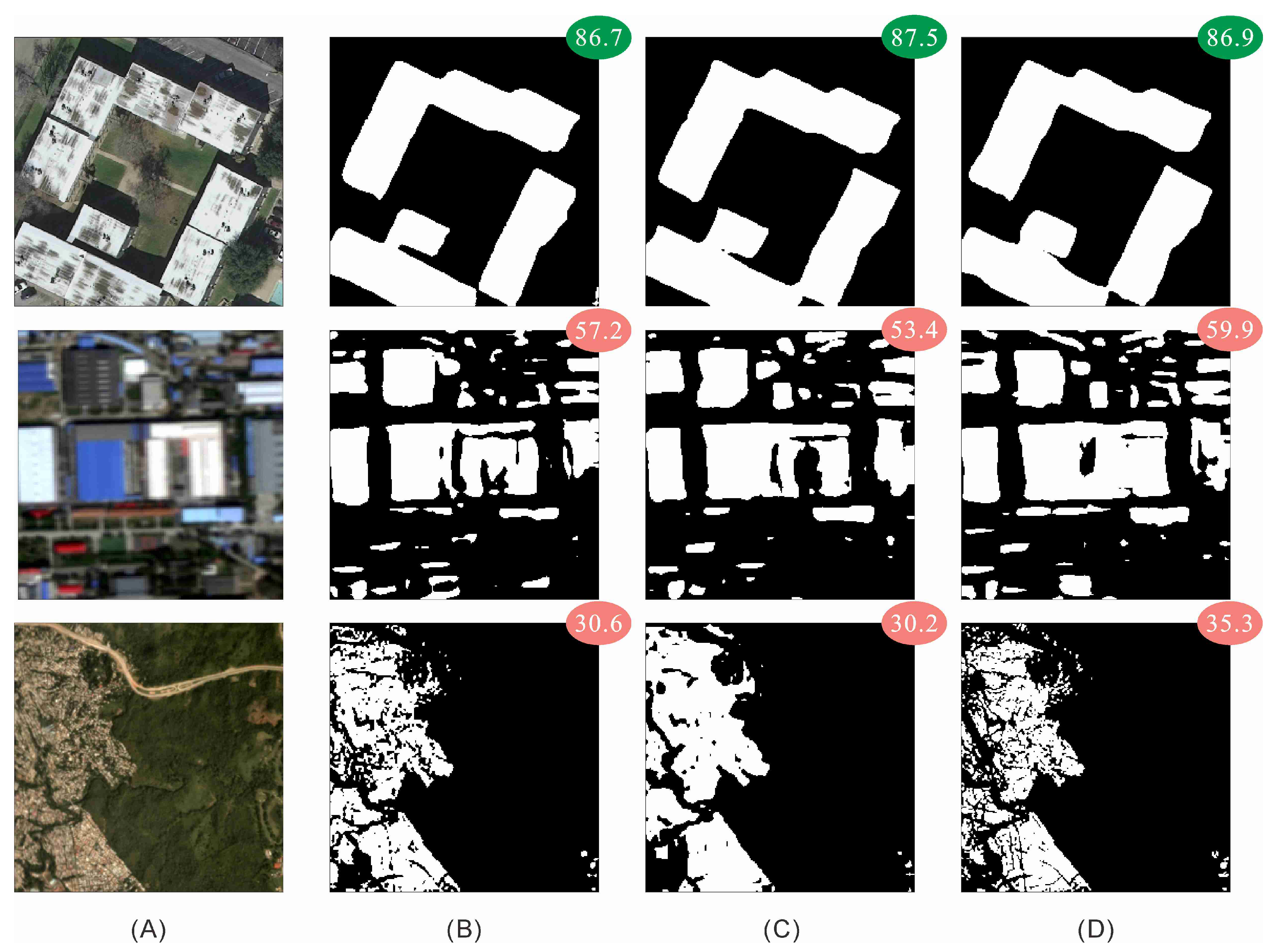
Existing segmentation techniques based on multi-level fusion have been proven effective with building extraction, particularly in HR images. However, when these algorithms are applied to LR images, the extracted building is not always sufficiently accurate to serve building-oriented applications. As shown in the first row of Figure 2, all models exhibit considerable accuracy in high-resolution scenes with little variation.
However, as the image resolution decreases to 4 m/pixel in the second row, the IoU score drops by approximately 30%, indicating more delineation errors. Specifically, errors primarily occurred on the boundaries. In the third row, where the image resolution is further reduced to 8 m, the model has difficulty locating buildings, particularly small buildings. The results show a gap in accuracy in predictions with HR and LR images. The paragraphs below detail potential reasons for these misclassifications.
First, low–high level semantics may not be accurately preserved in LR images. Due to the limited resolution, LR images contain more ambiguous information (e.g., mixed pixels), indicating that the original image (i.e., the lowest-level feature) contains irrelevant noise. The fuzzy semantics of non-building objects or background have a detrimental effect on prediction; therefore, it is essential to suppress the irrelevant noise in a self-adaptive manner to improve the segmentation accuracy.
A second issue is the confusion of fuzzy boundary details. To involve the boundary information, one always needs to use the boundary ground truth to provide additional supervision. In LR images, however, the buildings always have fuzzy boundaries (as seen in Figure 1B), and some boundaries even blend into the building background, appearing as a non-edge pixel. This causes ambiguity between the boundary ground truth and the boundary pixel. A more effective approach is to learn the features sparsely by concentrating on only the salient and representative portions of boundaries because the dense information propagation guided by the edge ground truth may be confused with other irrelevant details.
The third issue is the lack of local texture. Due to the low contrast, it is more challenging to capture texture details in LR images than it is in HR images. Akiva et al. [41] applied a pixel adaptive convolution layer [42] to introduce the texture from the input image, thus, refining deep features and encouraging the representation of pixels with similar signatures. Unfortunately, for building segmentation, involving the image texture would cause non-building targets to become prominent, leading to large intra-class variance. Utilizing non-local operation among different features to enlarge the model perception would be a more practical choice.
In this study, to address the fuzziness issue, we use the point-wise sparse propagating strategy instead of the dense propagating strategy (feature-wise) as in Equation (2). Specifically, we only calculate the affinity of representative feature points on the edges and corners of buildings (i.e., D l 1 ( p ) and D l ( p ) , p is the sampled pixels) in the two adjacent pyramid feature maps D l 1 and D l . The positions of the selected feature points are learned by the model. Then, we apply the proposed gated fusion module as an affinity function A to harvest the specific context only on selected edges and corners of buildings to alleviate the side effect of the fuzzy contexts in LR images:
D l 1 ( p ) = A ( E l 1 ( p ) , D l ( p ) ) D l ( p )
The differences among the three types of feature fusion design are shown in Figure 3. The innovation compared to other work is that we propagate the building feature contexts in a sparse way instead of in a dense way. Finally, for the lack of local textures, we harvest the global attention of the input using the recently introduced grounding transformer, in which the interactions between adjacent features are in a non-local style.

3. Sparse Geometry Feature Attention Network

In this section, we describe, in detail, the proposed SGFANet, including the overview (Section 3.1), the modules (Section 3.2 and the loss function (Section 3.4)).

3.1. Overview

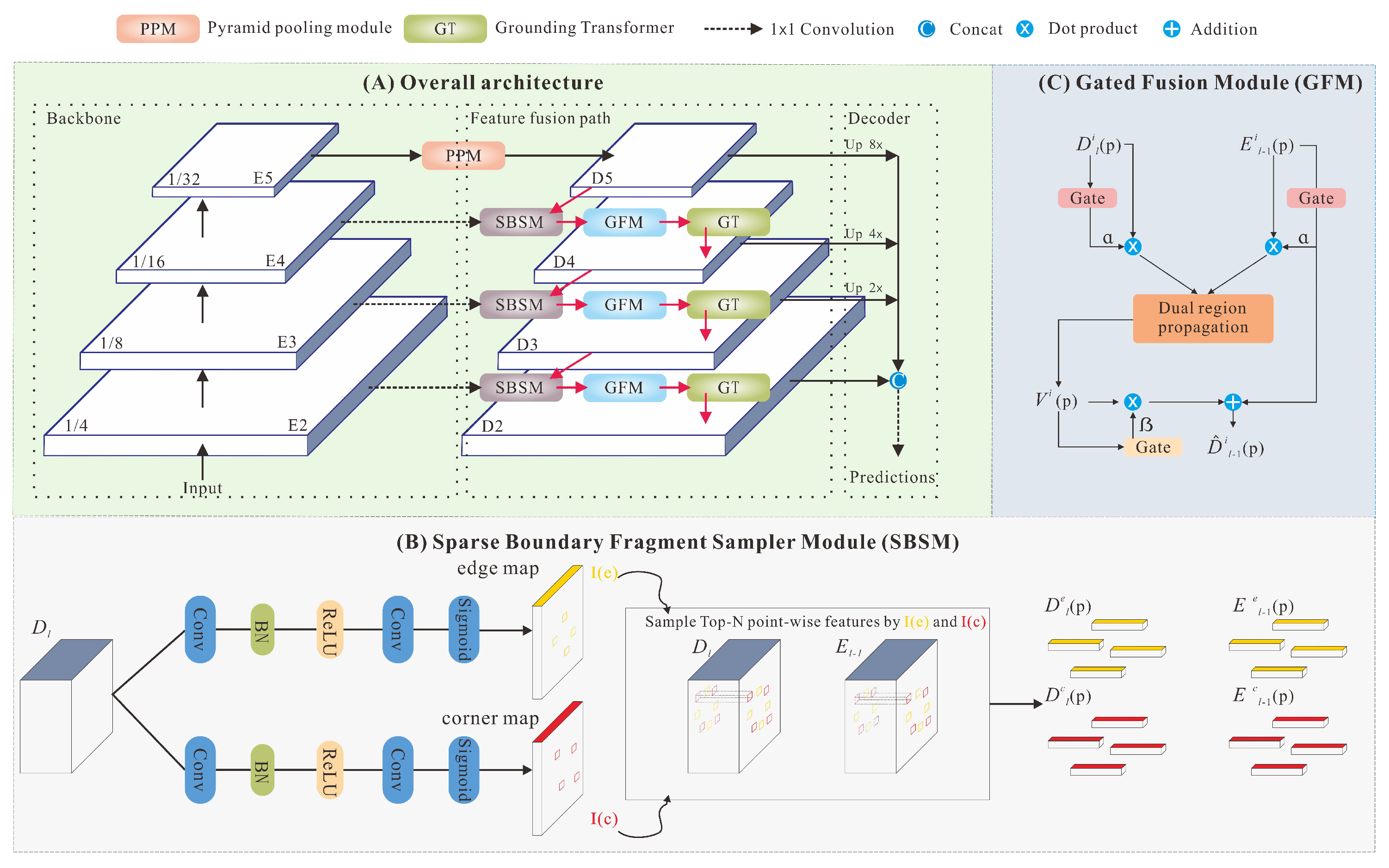
The proposed method is based on a bottom-up feature extractor and a top-down feature fusion path as shown in Figure 4. The choice of the feature extractor is not the focus of this study; thus, ResNet-50 [43] was implemented. The feature extractor produces a series of multi-level features that are denoted as E l | l = 2 , 3 , 4 , 5 . To enhance contextual semantics, we applied the pyramid pooling module (PPM) to the highest feature map E 5 and obtained the top pyramid feature D 5 . This is a widely used setup in various feature fusion methods [20,28,37,39].
Then, we fused the set of E l along with the building boundary feature in a top-down and sparse manner (i.e., focusing on the representative features to alleviate the irrelevant noises brought by fuzzy details). This process generates the pyramid feature set D l | l = 2 , 3 , 4 . Finally, we concatenated all pyramid features in D l to generate the building prediction result.

3.2. Learning Sparse Geometry Features

This subsection posits that the multi-level feature set, denoted as E l , and the highest-level pyramid feature, which is denoted as D 5 , have been successfully acquired by the ResNet-50 backbone and PPM module. Then, the proposed top-down fusion method is described in detail.

3.2.1. Sparse Boundary Fragment Sampler Module

Different from other methods [23,40], we propagate the edge and corner contexts separately and sparsely in a top-down manner. In this study, we argue that the most representative feature points can be represented as top-N points from the possibility maps of both edges and corners. We define “Top-N” as “the first N points with the highest possibility in the possibility map”, where N is a hyperparameter and can be different in edge and corner possibility maps (see more detail in Section 4.8).
As shown in Figure 4B, we propose the sparse boundary fragment sampler module (SBSM) to select the top-N feature points. The SBSM uses two independent branches over the pyramid feature D l to obtain the edge and corner possibility map of the input image. These two branches are both implemented by a 3 × 3 convolutional layer, a batch normalization layer, a ReLU function, and another 3 × 3 convolutional layer followed by a sigmoid function and are supervised by the ground truth of the edge and corner distribution map. Then, the SBSM samples the top-N points according to their possibility value to obtain the representative edge indices I e and corner indices I c .
Before obtaining the representative feature points, we first refine E l 1 using a 1 × 1 convolutional layer. Next, the SBSM obtains the representative feature points from D l and E l 1 according to I e and I c . We use the normalized grids and bilinear interpolation during the implementation. The representative edge feature points are denoted as D l e ( p ) and E l 1 e ( p ) , while the corners are denoted as D l c ( p ) and E l 1 c ( p ) .

3.2.2. Gated Fusion Module

After obtaining D l ( p ) and E l 1 ( p ) , the critical point is how to propagate them in the proposed fusion path. However, different levels of D l have different capacities to capture the edge and corner spatial and contextual information. Simply designing a uniform propagation mechanism for each level of the pyramid feature would produce a semantic gap; thus, we design an attention mechanism that serves as an affinity function to reweight the feature points from different levels and propagate them.
We propose a gated fusion module, which contains two parts: (1) a gated operator and (2) dual region propagation. The gated operator is a channel attention mechanism focusing on reweighting features along the channel of each pyramid level. It first explicitly models the dependency of features along the channel and learns a descriptor to express the importance of each channel. Then, the descriptor enhances the useful channel and suppresses the inferior channel by dot production. The gated operator is as follows:
D ˜ l i ( p ) = α l i ( p ) · D l i ( p ) E ˜ l 1 i ( p ) = α l 1 i ( p ) · E l 1 i ( p ) ,
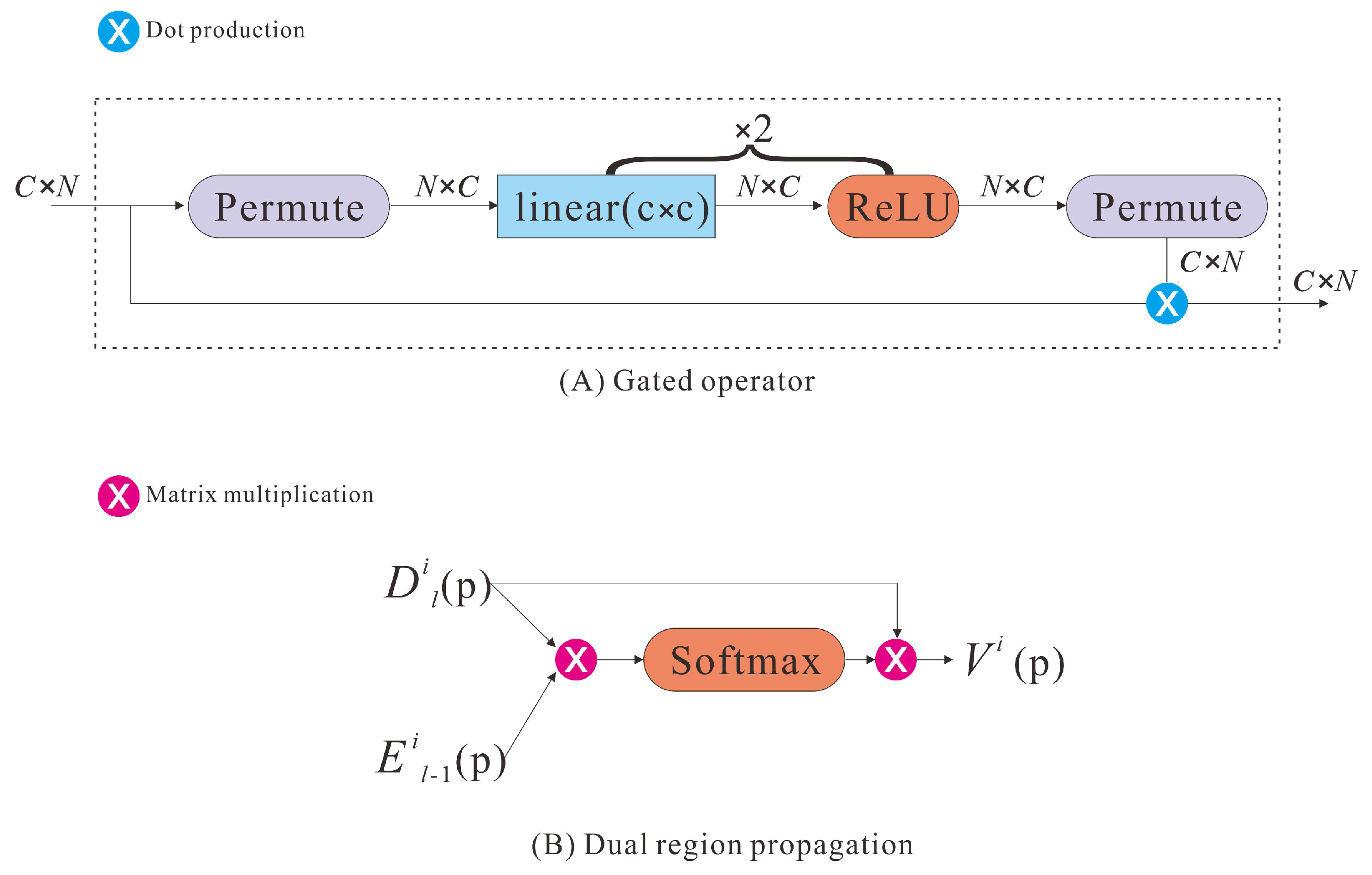
where i is the index from I e or I c ; α l i ( p ) [ 0 , 1 ] and α l 1 i ( p ) [ 0 , 1 ] are the associated gate maps of each level l, which are obtained through linear projection from D l i ( p ) and E l 1 i ( p ) , respectively; and · denotes the dot multiplication broadcasting in the channel dimension. More detail is available in Figure 5.
Then, we propagate those gated sampled features independently. For each group of sampled features (i.e., the edge or the corner), top-down propagation is realized by dual region propagation followed by another gated mechanism as shown in Equation (5):
V i ( p ) = δ ( D ˜ l i ( p ) × E ˜ l 1 i ( p ) ) × D ˜ l i ( p )
and (6),
D ^ l 1 i ( p ) = β i ( p ) · V i ( p ) + E ˜ l 1 i ( p )
where δ denotes the softmax function for value normalization; V i ( p ) is the affinity of D ˜ l i ( p ) and E ˜ l 1 i ( p ) ; × denotes matrix multiplication; · denotes the dot product; and β i ( p ) [ 0 , 1 ] is another gated operator obtained from the linear projection of V i ( p ) .
Equation (5) is the dual region propagation, which is a type of self-attention mechanism, and we only apply selected representative feature points to the calculation. Equation (6) is another gated operator that is used to filter out useless contexts. In this study, we use the residual design for easier training in Equation (6) (i.e., the add operation to accelerate gradient broadcast). The overall gated pipeline is shown in Figure 4C.

3.3. From Local to Non-Local Features

The CNN has been shown to be powerful in local features for its shared position-based kernels over a local and fixed-size window, which keeps the translation invariant and makes promising results in capturing local features, such as shapes [44,45]. Unfortunately, the LR image lacks local texture details due to the low contrast. If we focus on the local pattern, as conventional CNN does, the learning procedure in a low-resolution plane would be insufficient. To combat this issue, we transfer the local calculation to non-local operation using the recently introduced grounding transformer (GT) [20]. In this study, we use two convolution layers on D l to obtain q and v and one convolution layer on E l 1 to obtain k. q, k, and v denote the key, query, and value in the transformer, respectively. Then, we implement the GT as:
s = q · k w = δ ( s ) D ^ l 1 = w × v
where δ is the softmax function, and the output of the GT is denoted as D ^ l 1 , which harvests the nonlocal contexts (i.e., global) of two adjacent pyramid features (i.e., E l 1 and D l ). Finally, the refined output feature D l 1 is obtained by scattering the feature point D ^ l 1 i ( p ) into D ^ l 1 according to the indices I e and I c . The top-down procedure is summarized in Algorithm 1.
Algorithm 1: The top-down procedure in SGFANet.
Require: 
E l | l = 2 , 3 , 4 , 5 : the extracted feature set from the backbone; N c : the sampling number of corner points; N e : the sampling number of edge points; and D 5 : the highest-level pyramid feature.
Ensure: 
The pyramid feature set D l | l = 2 , 3 , 4
1:
forl in [5, 4, 3, 2] do
2:
     e d g e _ m a p , c o r n e r _ m a p Sigmoid (Convolution( D l ))
3:
    Obtain I e and I c from e d g e _ m a p and c o r n e r _ m a p
4:
     D l e ( p ) , D l c ( p ) Grid_sample ( D l , I e ), Grid_sample ( D l , I c )
5:
     E l 1 e ( p ) , E l 1 c ( p ) Grid_sample ( E l 1 , I e ), Grid_sample ( E l 1 , I c )
6:
     D ˜ l i ( p ) Gated_operator ( D l i ( p ) ) with Equation (4)
7:
     E ˜ l 1 i ( p ) Gated_operator ( E l 1 i ( p ) ) with Equation (4)
8:
     D ^ l 1 i ( p ) Dual_region_propagation ( E ˜ l 1 i ( p ) , E ˜ l 1 i ( p ) ) with Equations (5) and (6)
9:
     D ^ l 1 Grounding_transformer ( E l 1 , D l ) with Equation (7)
10:
   D l 1 Scatter the D ^ l 1 i ( p ) into D ^ l 1 according to the I e and I c .
11:
end for
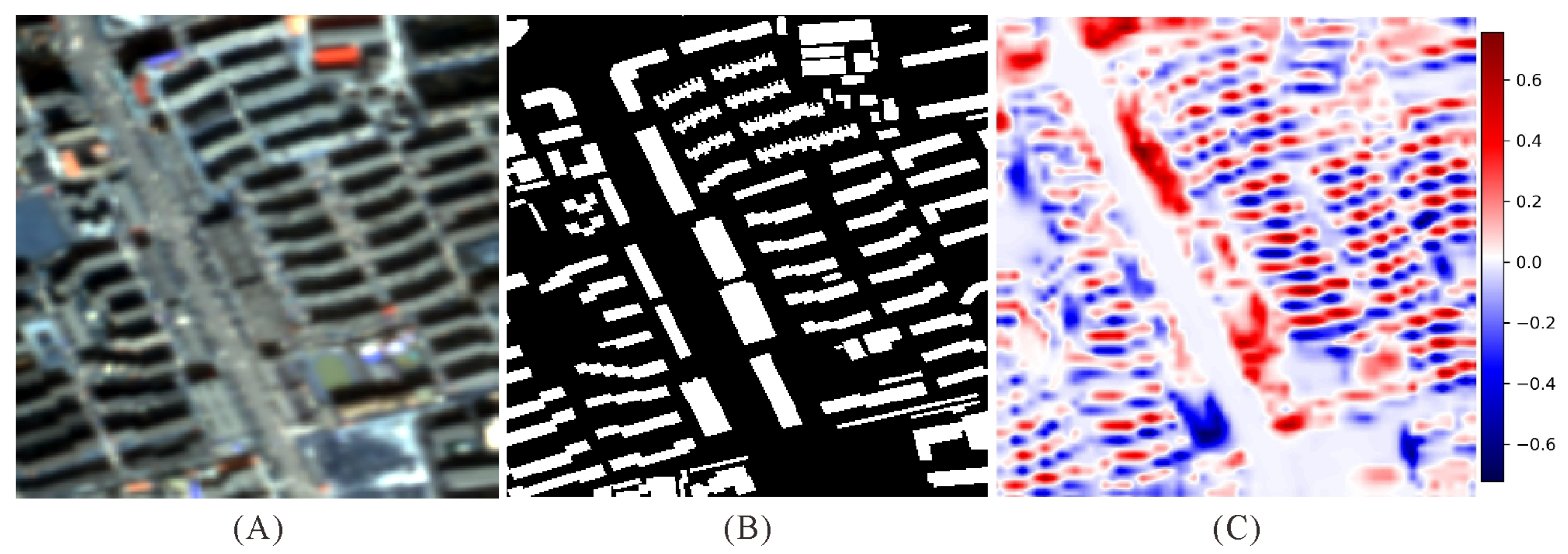
As previously described, CNN is limited by its locality when resolving LR images. As we want to emphasize nonlocal attention to compensate for the lack of local texture, we use GT to fully interact with the pyramid feature in both spaces and scales. When using GT, the model encourages representation consistency for the building region and inhibits the false alarms of the building background as shown in Figure 6.

3.4. Decoder and Loss Function

The decoder is used to recover the spatial resolution of the output feature D l | l = 2 , 3 , 4 , 5 R C × H × W . We adopted a simple and lightweight decoder in SGFANet to preserve the model’s efficiency. SGFANet concatenates all the refined D l by upsampling them to the same resolution (1/4 resolution of the input image) and performs the final prediction by a 1 × 1 convolutional layer and sigmoid function.
The overall output of SGFANet is threefold: the edge confidence map, the corner confidence map, and the final segmentation prediction map. We, thus, use binary cross entropy as a loss function, and these losses are weighted to 1 by default.

4. Experiments

4.1. Definition of LR and HR Images in This Paper

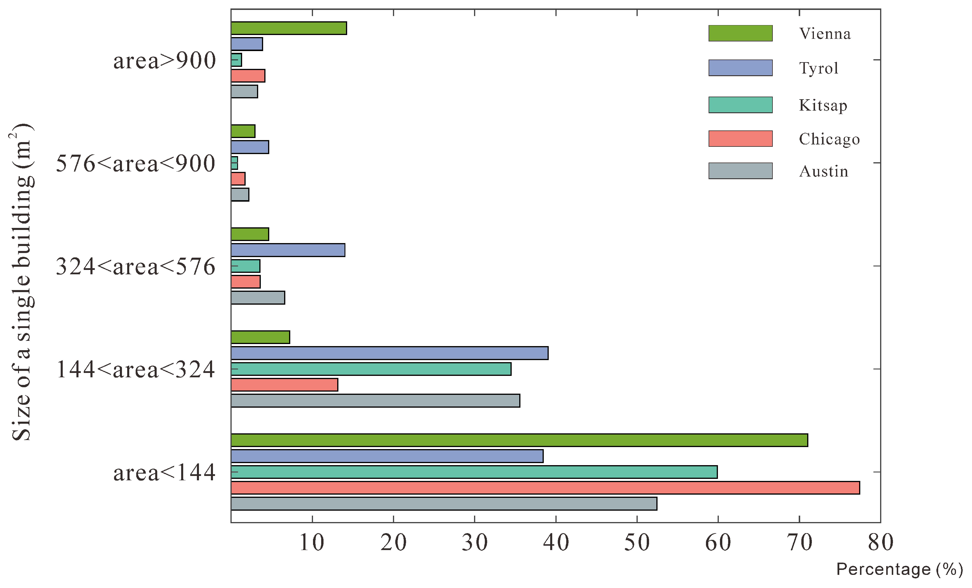
To segment individual buildings, the definitions of LR and HR are different from those of other tasks [46]. As shown in Figure 7, most buildings are under 144 m 2 . Assuming a resolution of 4 m/pixel, up to nine pixels are used to render one building. Convolutional layers with 3 × 3 kernels are the foundation for contemporary deep-learning segmentation models. Due to the small size of the building, a sliding window could not be filled in one convolutional layer, introducing a great deal of background noise into building segmentation. In addition, the geometric components of buildings (e.g., the edges and corners) are small and could blend into the background. Accurate building segmentation could, thus, be strongly hampered by these confusing pixels. Xu et al. [18] and Zhang et al. [15] defined 1.2, 2, and 4 m/pixel as low resolution, while Shi et al. [47] defined 3 m/pixel as moderate resolution. In this study, the LR images are those with a resolution of greater than 4 m, while the HR images are the reverse.

4.2. Datasets

To demonstrate the effectiveness of the proposed methods, we have three goals: (1) to assess the performance of SGFANet on LR images and other existing methods; (2) to assess the performance of SGFANet as an SS module under the existing SR-then-SS framework; and (3) to assess the effectiveness of the proposed module and evaluating how different combinations affect the model performance.
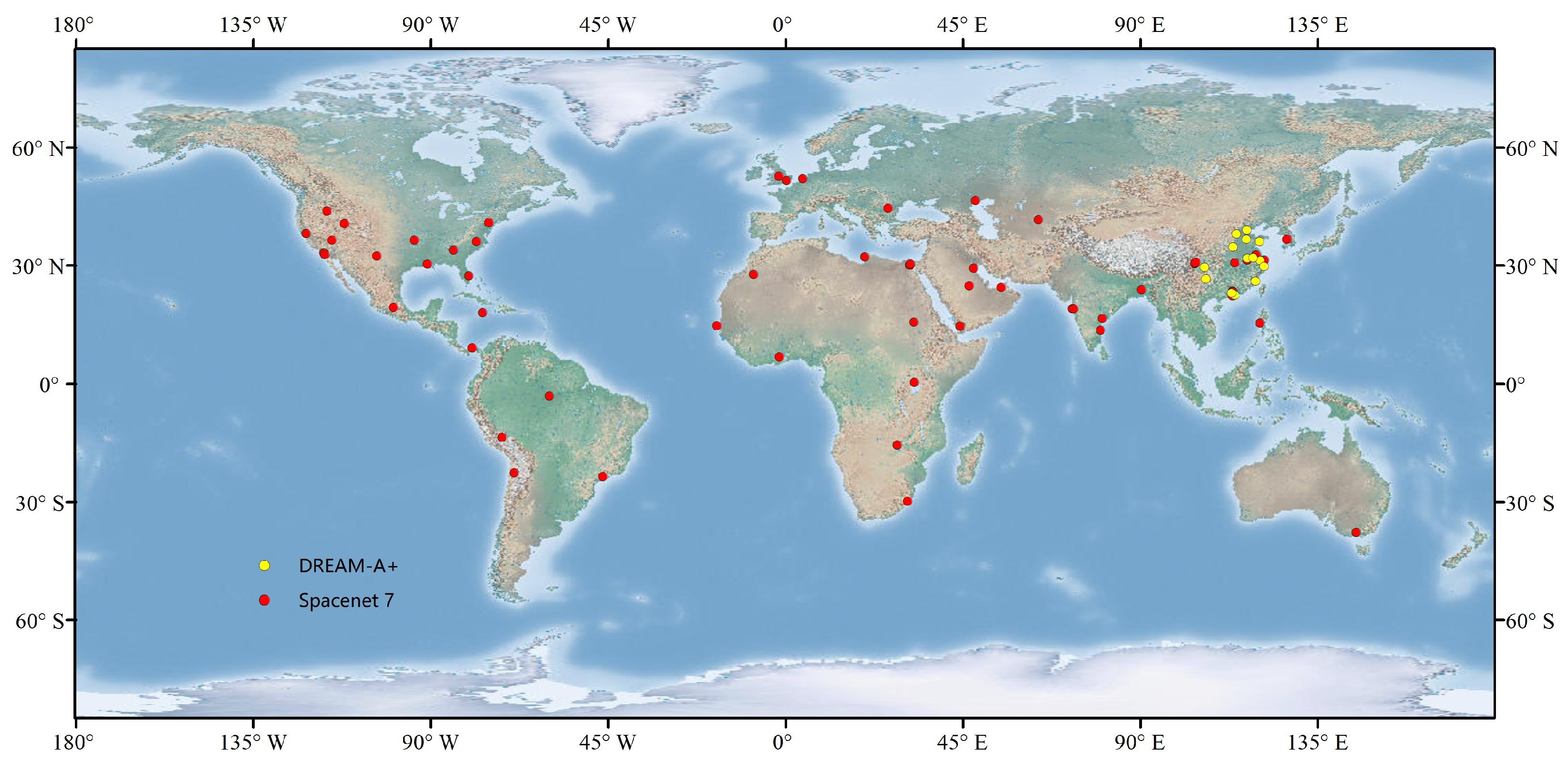
We used two datasets: the Multi-Temporal Urban Development Spacenet (i.e., Spacenet 7) and the DREAM-A+ dataset [18,19]. Spacenet 7 provides 4 m/pixel RGB imagery and the corresponding building footprint in GeoJSON format. The released images and the ground truth were captured in 60 locations worldwide. Each location provided 24 images (one per month) with a size of 1024 × 1024 between 2017 and 2020, covering an area of approximately 18 km 2 . The DREAM-A+ dataset contains 4 m/pixel RGB imagery captured by the Gaofen-2 satellite sensor as well as the corresponding building footprints in Shapefile format. The images are presented as 256 × 256 image patches that were uniformly collected across 14 cities in China. The distribution of the data samples is shown in Figure 8.
In addition, we collected the corresponding low-resolution imagery with RGB and NIR bands from Sentinel-2 (10 m/pixel). The images were obtained in the same period and location as the corresponding image in Spacenet 7 and DREAM-A+. Images with an excessive amount of clouds (e.g., 20%) were omitted from the Sentinel-2 dataset, reducing the amount of available imagery. Then, by rasterizing the related GeoJSON and Shapefile, we matched each Sentinel-2 image with a 2.5 m building ground truth.
With these datasets, we conducted three types of experiments. First, we evaluated SGFANet compared to existing methods on Spacenet 7 and DREAM-A+, which we merged into one dataset. This scenario is closer to practical applications (i.e., satellite images derived from multiple sensors and geographic locations), which requires higher generalization performance of the model. Second, we evaluated the SGFANet performance in the SR-then-SS framework on the collected Sentinel-2 imagery. Sentinel-2 imagery is publicly accessible from most places around the globe; therefore, it is practicable to use only this sensor. Third, we verified the proposed module utilizing the DREAM-A+ dataset. In this experiment, we were concerned with the effect of various modules on the model performance; thus, we used a single source image to make the experiment reliable.

4.3. Implementation Details

We cropped the 4 m/pixel images into a fixed size of 256 × 256 and the 10 m/pixel images into the size of 64 × 64. In the process of training, the AdamW [48] optimizer was used with a 0.001 learning rate, and the method was trained for 100 epochs on image tiles. The batch size was 16. In each mini-batch, we used standard data augmentation with a probability of 20 % , including rotation of [ 20 , 20 ] , horizontal and vertical flip during training. For hyperparameter N, we adopted 128 and 32 for sampling points from the edges and corners, respectively.
The threshold of the sigmoid output was 0.5. The layers in Resnet-50 were initialized with the pre-trained weight on ImageNet. The training, validation, and test set were randomly divided in a ratio of 5:2:3. The number of image tiles in each set is shown in Table 1. During training, we assumed that the test set was invisible. After each epoch, we verified the accuracy of the model on the validation set and chose the model with the highest accuracy in the validation set for testing. Unless otherwise stated, the precision we report in the experiment is the precision of the test set. All experiments were implemented in PyTorch.

4.4. Accuracy Assessment

Four evaluation metrics were used to assess the performance of the models, including the intersection over union (IoU), overall accuracy (OA), F1 score (F1), and boundary F1 score (b-F1). After obtaining the prediction maps, true-positive (TP), false-positive (FP), true-negative (TN), and false-negative (FN) pixels were calculated. True positives mean the truly predicted pixels with positive labels, and false positives denote negative labels with false predictions. For IoU, OA, and F1, the positive pixels are the building regions. For b-F1, the positive pixels are building boundary pixels. The evaluation metrics are calculated as follows:
I o U = T P T P + F P + F N O A = T P + T N T P + F P + F N + T N F 1 = 2 × T P 2 × T P + F P + F N

4.5. Results of SGFANet

Using the collected 4 m/pixel images, we compare the proposed SGFANet with several literature works to assess its effectiveness on the semantic segmentation task, including state-of-the-art (SOTA) methods, the dense boundary propagation method, and the shape-learning method:
  • DeepLabV3+ [49] achieved SOTA results in the PASCAL VOC dataset. It is also a common baseline method in the semantic segmentation field.
  • Unet++ [38] is the SOTA architecture among variants of the Unet. Its multi-scale architecture makes it effective in capturing various sized targets and is, therefore, often applied in building extraction.
  • ICTNet [31] was the winner in the 2019 INRIA competition. It utilizes dense-connection block [50] to extract building features. Instead, our method adopts a sparse propagation strategy supervised by the building boundary label.
  • CBR-Net [34] achieved SOTA results in the WHU building dataset. It is also the most recent SOTA algorithm.
  • PFNet [37] achieved SOTA results in the iSAID dataset. It is not dedicated to extracting buildings; however, it uses a sampling strategy similar to ours. The greatest difference is that it samples mainly to tackle the imbalance between the foreground and background pixels, while we are more refined, targeting only the building boundary and corner pixels.
  • EPUNet [40] is a dense boundary propagation method. Compared with ICTNet, it introduces building boundaries as supervision. Compared with our method, it propagates the boundary contexts densely (i.e., without any context filtering).
  • ASLNet [27] is a shape-learning method that applies the adversarial loss as a boundary regularizer. It is designed to extract a more regularized building shape.
For the comparison methods, we used the hyperparameter settings from their respective studies (e.g., the dimensions of the convolution filters). To create fair comparisons, other training parameters, such as the backbone network, learning rate, and batch size, were kept consistent with the proposed approach.

4.5.1. Comparison with State-of-the-Art Methods

The quantitative evaluations of the proposed SGFANet and other existing methods are listed in Table 2. The proposed SGFANet outperformed the other methods by a wide margin. DeepLabV3+, Unet++, and PFNet were initially proposed for segmentation on general segmentation tasks but do not consider special issues in segmentation on building extraction and achieved lower accuracies than SGFANet. ICTNet was designed to use the compact internal representation of the backbone network and dynamic attention mechanisms in the decoder network to extract buildings in HR images well.
However, ICTNet’s lack of explicitly modeling the LR issues makes it inefficient compared to the proposed method. The CBR-Net is built upon a coarse-to-fine framework by simultaneously taking several sources of prior information about buildings (e.g., the boundary directions). Unfortunately, in LR images, this prior information is less marked than that in HR images due to less detailed spatial information, which poses a weak supervision problem for CBR-Net. Compared with CBR-Net, our method achieved 0.66%, 0.21%, 0.60%, and 0.21% improvement on IoU, OA, F1, and b-F1, respectively.
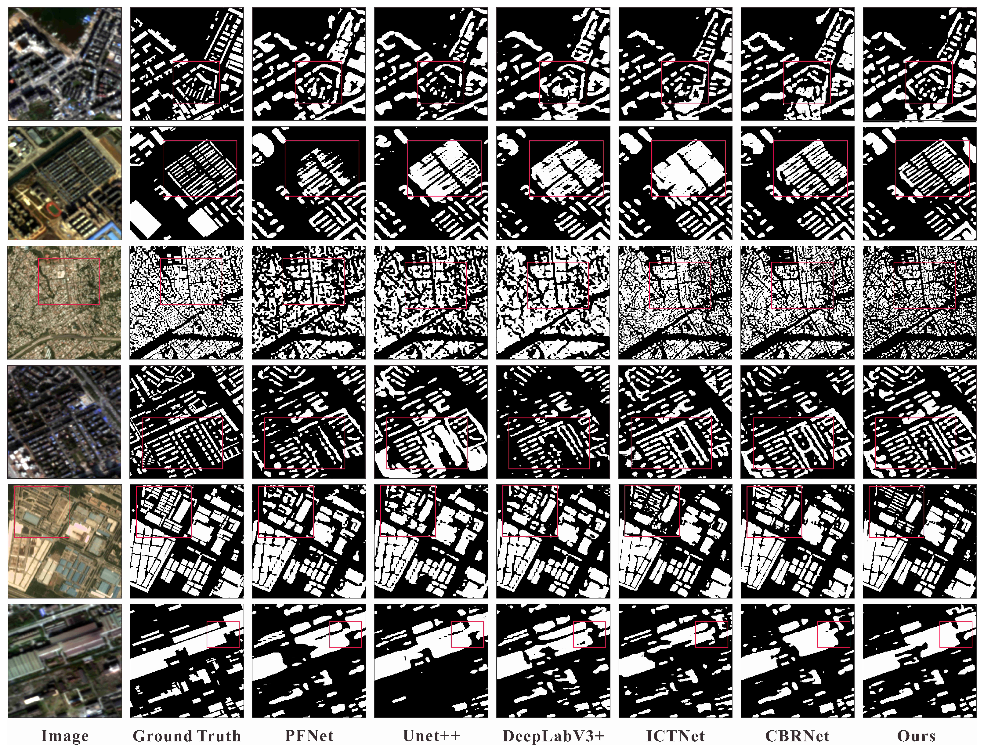
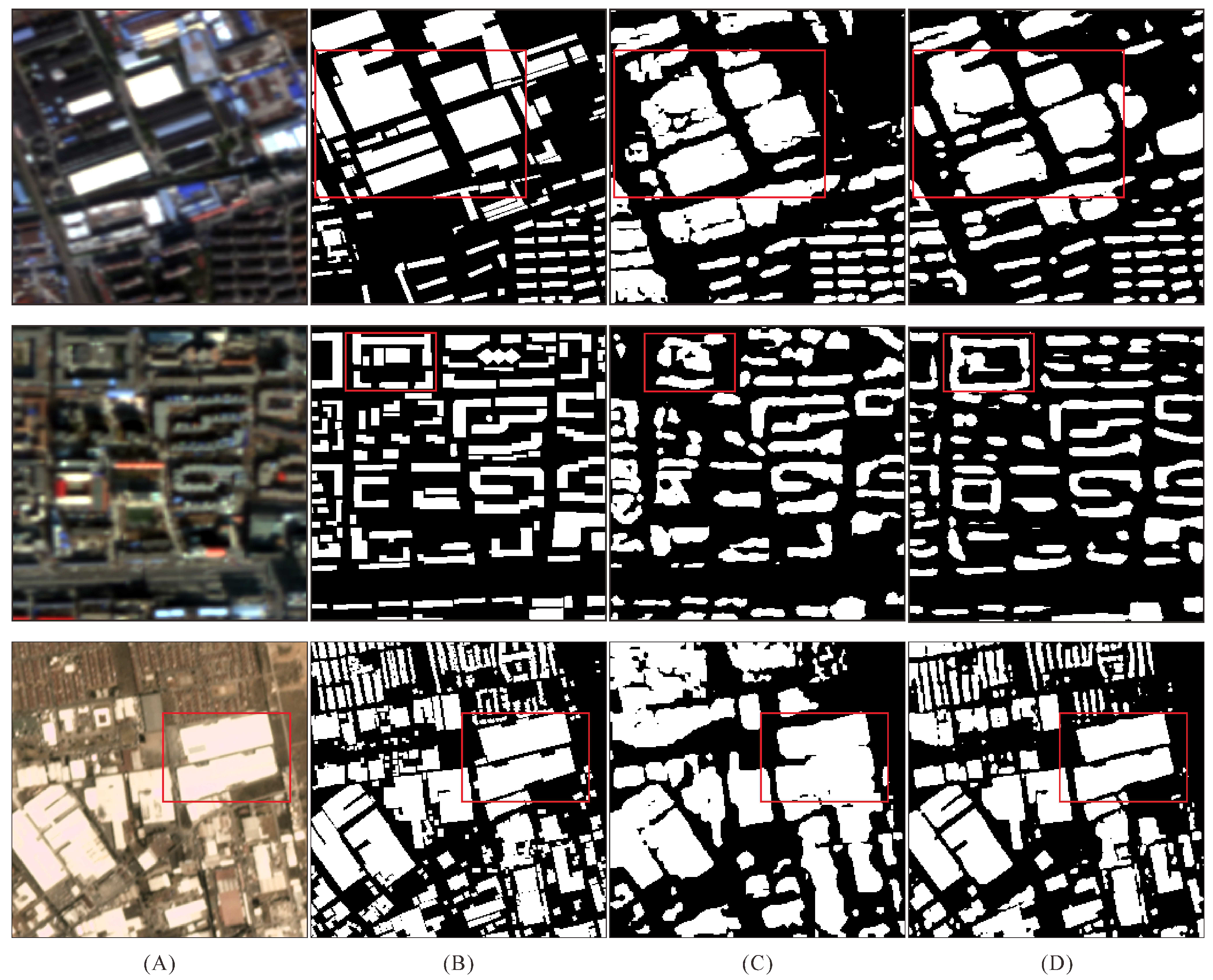
Qualitative results are shown in Figure 9. Due to the image’s low resolution, the building in it is smaller and more difficult to distinguish. However, the proposed SGFANet still had better segmentation results in handling false-positives of dense building regions and a better capability to extract high-quality building boundaries compared with the other methods. Specifically, the proposed SGFANet had several advantages in different scenes. The method could accurately extract individual buildings from the first row to the third row of Figure 9.
When the building boundary becomes much fuzzier in the fourth row, the proposed method still produced accurate predictions, while the other compared methods failed to manage this change. The segmentation results of the proposed method have fine-grained boundaries in the fifth and sixth rows, while other methods may generate blob-like results. Notwithstanding the advancements achieved by our proposed technique, the extent of progress in the small-sized building extraction remains constrained as illustrated in (Figure 10). While SGFANet successfully identified small buildings, it faced difficulties in accurately outlining their boundaries. This inadequacy can be mainly attributed to the comparatively smaller dimensions of these buildings, resulting in an imbalanced training set with fewer pixels available for training.

4.5.2. Comparison with Dense Boundary Propagation Methods

We further compare our method with a dense boundary context propagation method, the EPUNet [40], which adopts the opposite strategy to ours in handling the boundary supervisions. The EPUNet achieved promising results on HR remote sensing benchmarks, such as the WHU Building Dataset (0.3 m/pixel) and SYSU Building Dataset (0.8 m/pixel) with 7.47% and 2.86% accuracy gaps of IoU compared with DeepLabV3+ as reported in Guo et al. [40]. However, in our experiment, when the resolution was reduced to 4 m/pixel, the accuracy of EPUNet dropped by a large amount and approached that of Deeplabv3+ (see in Table 2).
We propose that the dense propagation of edge information brings too many fuzzy contexts to the prediction, and this phenomenon was more significant when the resolution decreases. The proposed SGFANet propagates the building boundary information (i.e., the edges and the corners) sparsely by the proposed SBSM and the GFM. As seen in Table 2, our result outperformed EPUNet by 2.62%, 0.92%, 2.41%, and 1.49% at IoU, OA, F1, and b-F1. Additionally, when buildings are densely distributed, the EPUNet tends to obtain ambiguous predictions of building boundaries, while we could more reliably detect boundary pixels from this dense area (see in Figure 11).

4.5.3. Comparison with Shape Learning Methods

Recent studies in building extraction have used shape constraints as an additional loss to optimize the training procedure, particularly when employing HR images [26,27,51]. ASLNet [27] uses adversarial loss [52] to determine whether the morphology of the model output is consistent with the ground truth and, thereby, achieves good performance that is comparable to those of other generative adversarial network (GAN)-based methods. However, ASLNet struggles to appropriately capture building shape when it meets with LR imagery. As shown in Table 2, our method improved 7.99%, 1.27%, 6.99%, and 6.76% in terms of the IoU, OA, F1, and b-F1, respectively. In Figure 12, the ASLNet did not converge as well as expected and therefore output blob-like results. This result likely occurred because the LR images typically have unclear building shape patterns due to confusing pixels, providing the model with less effective shape information for optimization.

4.6. Super Resolution and then Semantic Segmentation

4.6.1. Framework Architecture

Without a loss of generality, we used the commonly used baseline method from the SR field of research (i.e., the efficient subpixel convolutional neural network (ESPCN) [53]) as our SR module. Following the previous well-established experimental setting [18], we used the SR as the front component and the SS as the rear component. Specifically, the input LR imagery was first processed by the SR to output the upsampling feature. Then, the SS was fed the generated upsampling feature to obtain an upsampling prediction result. In this experiment, we kept the SR module invariant and only replaced the SS module with the model mentioned in Section 4.5 and conducted experiments on the collected Sentinel-2 imagery.
Additionally, to comprehensively evaluate the performance, we introduce two additional comparison methods:
(1)
ESPC_NASUnet [18] realizes the SR by ESPCN and the SS by NASUnet [54].
(2)
FSRSS-Net [19] introduces successive deconvolution layers in Unet, thus, achieving super resolution results.

4.6.2. Results

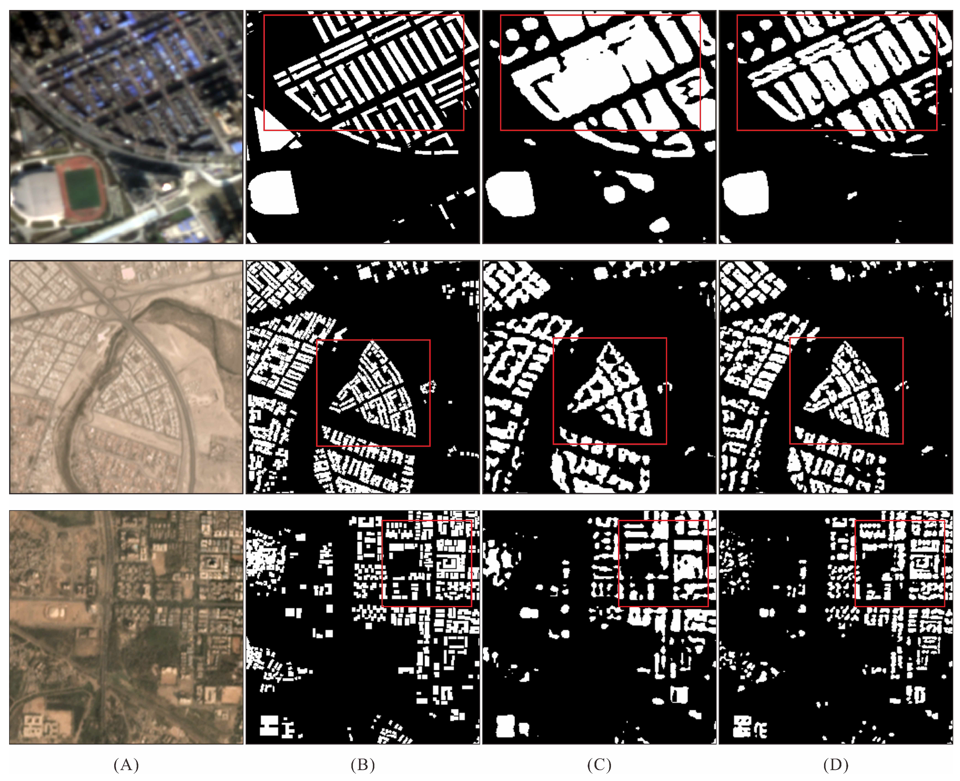
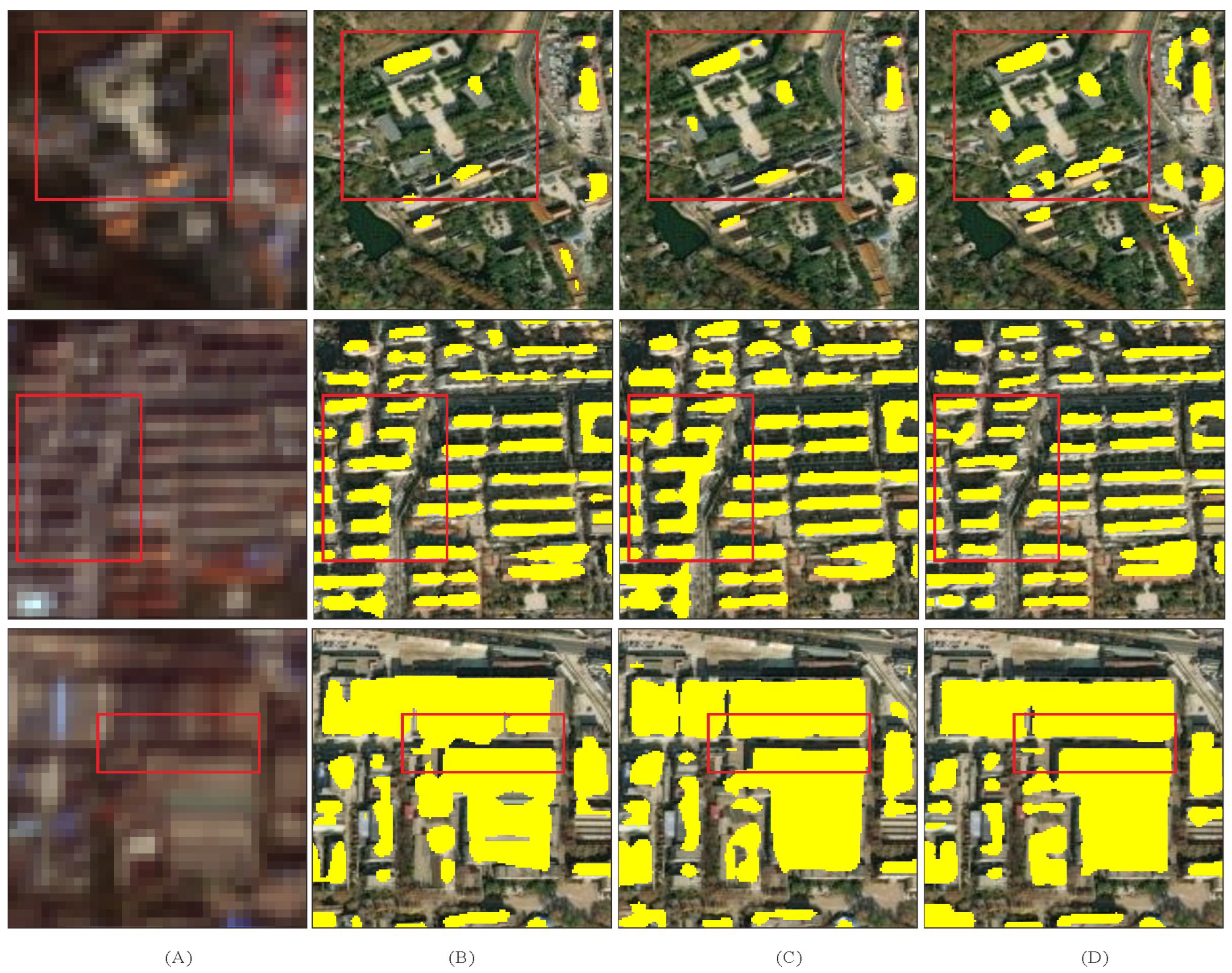
The quantitative results and the qualitative results are shown in Table 3 and Figure 13, respectively. From the quantitative perspective, with the SR module plugged in at the front, SGFANet still outperformed existing semantic segmentation methods and performed markedly better than the other two existing methods, achieving 2.74%, 1.49%, and 3.16% improvements in IoU, OA, and F1. From the qualitative perspective, the proposed method maintained accurate building boundaries while improving the segmentation of single buildings in dense residential areas.

4.7. Model Efficiency

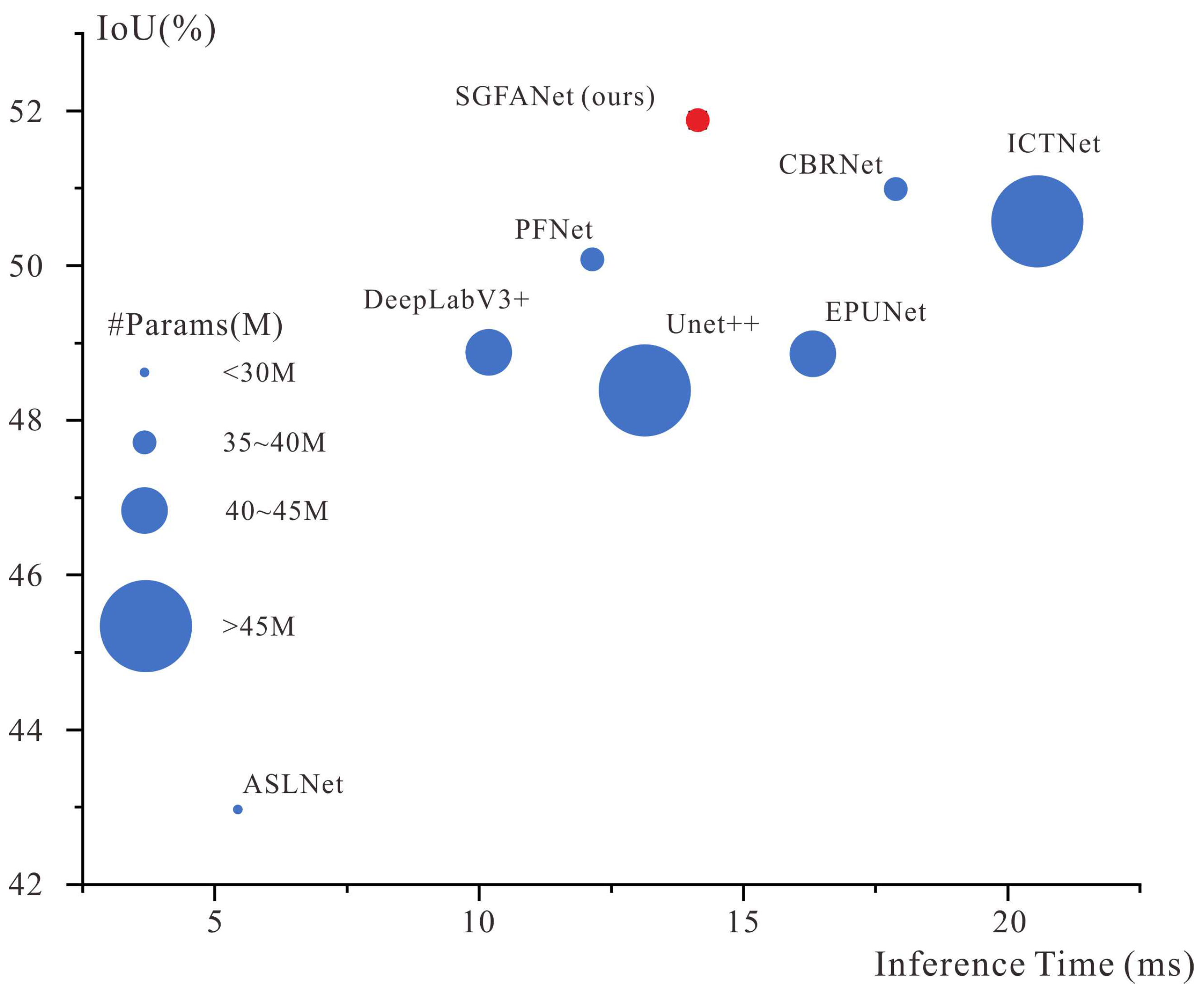
Figure 14 shows the trade-off between speed and accuracy. SGFANet outperformed methods with comparable parameter sizes, such as PFNet and CBR-Net, and achieved a higher efficiency improvement than did ICTNet (1.77 % in IoU). Thus, the proposed method achieved the optimal balance between speed and accuracy on the proposed benchmark.

4.8. Sampling of Edge and Corner Points

The number of sampled feature points about the edge ( N e ) and the corner ( N c ) impact the model performance. Due to the presence of these two parameters, it would be laborious to find their optimal combination during training. Although several parameter optimization approaches [55], such as grid search, random search [56], and genetic algorithms [57], have been shown to be useful in deep learning, directly using them would markedly increase the computational load.
In this study, we propose three straightforward and intuitive strategies for selecting the optimal number of sampled edges and corners: (1) sample only the edge points first and look for the best N e , and then adjust N c based on the best N e ; (2) sample only the corner points first and look for the best N c , and then N e is adjusted based on the best N c ; and (3) keep the ratio of N e and N c constant and adjust N e and N c concurrently.
We conducted experiments with these strategies separately on the DREAM-A+ dataset. As reported in Figure 15, different strategies obtained different trained results with different times. Table 4 reports the results on DREAM-A+ t e s t of these three sets of parameters, where “S1”, “S2”, and “S3” denote the adjusting strategy used, and the column “Time” is the rough cost time to adjust N e and N C on a single V-100 GPU. Considering the trade-off between accuracy and time cost, we recommend the third strategy, as mentioned above, for selecting the optimal N e and N c combination.
In Figure 15, if less appropriate parameter values are chosen, the accuracy of SGFANet decreases considerably. Thus, three configurations degrade the accuracy: (1) only sampling the corner or edge points; (2) undersampling the edge and corner points; and (3) oversampling the edge and corner points. These results verify that both edge and corner supervised information are equally important and indicates that sparse sampling (i.e., only sampling corners and edges simultaneously) is the bottleneck of LR image building segmentation because too little sampling leads to insufficient supervision, and too much sampling introduces too many fuzzy boundary contexts from LR images.

4.9. Ablation Study

In this subsection, we present comprehensive experiments to analyze the proposed modules in SGFANet. All experiments were conducted on the DREAM-A+ dataset.
The baseline of the ablation studies was the vanilla FPN architecture [35]. We ablated four modules in SGFANet: the pyramid pooling module (PPM), sparse boundary sampling module (SBSM), gated fusion module (GFM), and grounding transformer (GT). Table 5 reports the ablation results, where the baseline from the proposed method is the initial row. From top to bottom, the proposed modules are added in different combinations for the module analysis.
The PPM is essential for the feature fusion architecture, which achieved 0.26% improvement in IoU. The SBSM and GFM improved the IoU by 2.51% due to better boundary prediction as verified in Table 6. The primary improvement of GT lies in the undersegmentation of the building area. As a result, baseline+PPM+SBSM+GFM+GT achieved an IoU result with 0.67% improvement and an F1 result with 0.58% improvement compared with the baseline+PPM+SBSM+GFM. The gradual improvement in accuracy is indicative of the complementary property of the proposed method.
To demonstrate the effectiveness of the proposed modules, we verified the boundary improvements using the boundary F1-score metric (b-F1) with three different pixel thresholds in Table 6. Adding GT did not greatly improve the boundary predictions, which suggests that GT should primarily be used to capture the global attention of the image. By further applying SBSM, the boundary accuracy improved almost 1%. Moreover, as noted in the last row, adopting GFM resulted in much better results compared with the other designations. Empirically, using the gated operator is essential to preserve high-quality boundary information due to its ability to filter the boundary contexts in a top-down manner.
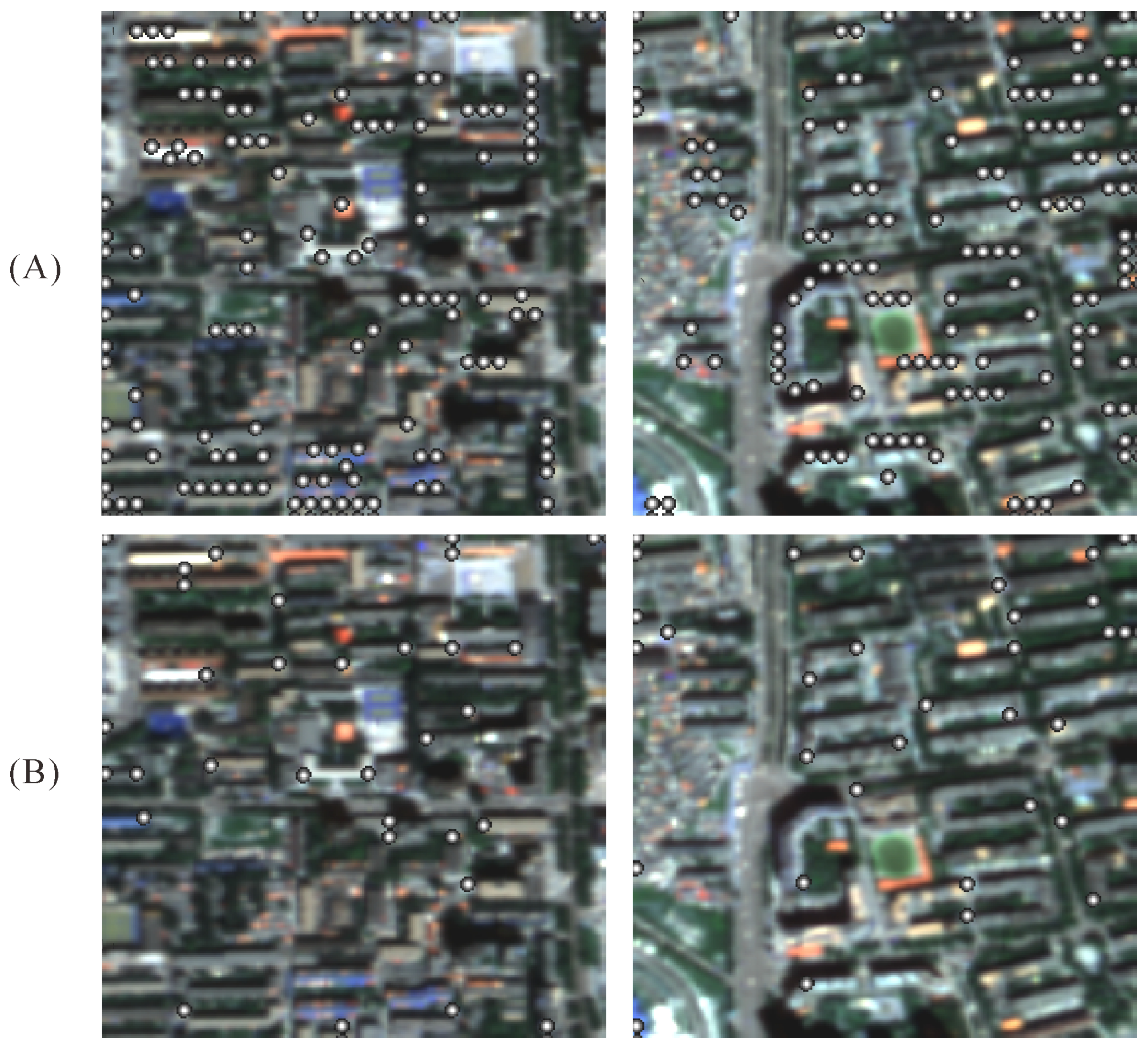
In Figure 16, we show two examples of the locations of the sampled edges and corner points on the original images by visualizing the points from the feature fusion path in the last stage. The positions of the sampled points indicate the representative and salient parts of the building boundary learned by the model. The GT was introduced to capture the non-local (i.e., global) attention of the image. We perform subtraction between the prediction score of SGFANet and that of SGFANet without the grounding transformer. As shown in Figure 6, GT can significantly improve the predicted score of the building region and inhibit the false alarms of the building background. Since the improvement is homogeneous on building predictions, in terms of evaluation metrics, GT brings the improvement of IoU rather than the b-F1 score as Table 6 indicates.
As a conclusion of the ablation study, the proposed modules in SGFANet have three benefits: (1) the sampling process in the SBSM and the gated operator in the GFM preserved high-quality boundaries in building segmentation by alleviating the fuzzy boundary detail from LR remote-sensing imagery; (2) the GT improved the building region predictions and inhibited background noise by introducing global attention to the input; and (3) SBSM, GFM, and GT were complementary to each other, and using these modules concurrently achieved much better performance than using the proposed baseline method.

5. Pilot Application: Dynamic Building Change of the Xiong’an New Area in China

In our benchmark, SGFANet achieved promising results in building segmentation from low-resolution remote-sensing images and improved the extraction accuracy in the SR-then-SS framework, thus, assisting in extending the accessibility and scalability of building dynamic tracking. We demonstrate this capability in this study with one example by presenting the dynamic building change in the Xiong’an New Area in China.
The Xiong’an New Area (XNA) plan [58] was initiated by the Chinese government on 1 April 2017. The XNA plan is a national strategy aimed at relieving the pressure on the Chinese capital city Beijing by migrating “noncore” functions. Large-scale construction activity has occurred in this 2000 square kilometer area since 2017.
Traditionally, there are two alternatives for building tracking. The first is to use HR images (e.g., the metric) to identify single-building-level changes [59], and the second is to use LR imagery (e.g., the decametric) to identify human settlement changes [60] or land-cover changes [61]. Existing research indicates that the high acquisition cost and low time availability of HR images make them problematic for large-scale applications. In addition, for LR imagery, it is challenging to detect changes at the level of individual buildings. Therefore, we would like to address the aforementioned issue using free LR data to enable the tracking of HR building changes.
We used publicly available Sentinel-2 images collected from the GEE platform to implement building-change detection at the annual scale from 2016 to 2021. We extracted the buildings for each year utilizing SGFANet with ESPCN (Section 4.6). Figure 17 shows the final building-change-detection results obtained after a time series analysis of the building distribution maps. The building construction and demolition activities were concentrated in three primary regions, as the red rectangle indicates.
Figure 17A shows the process of the demolition of some small villages and the construction of modern apartments. Between 2019 and 2021, some small settlements were progressively abandoned, and high buildings were created during 2020–2021. In Figure 17B, the process is nearly identical, with demolition occupying the vast majority of the area beginning in 2020, indicating that more construction is planned for the area. Figure 17C shows the building process of Xiong’an Railway Station, which was under construction in 2018 and operational in 2020.
As reported by the statistical curve in Figure 17, construction began as early as 2018–2019, while demolition activity peaked in 2020–2021. Compared to 2016, 1.2% of buildings were constructed, and 4.1% were demolished. The trend of the curve indicates that the construction and demolition process will continue in the future.
To verify these results, we calculated the temporal correlation coefficients (2016–2021) on the number of foreground pixels of the results with three well-acknowledged products: (1) the Dynamic World product (https://dynamicworld.app/, accessed on 23 March 2023), providing global land coverage at a 10 m resolution from 2015 to the present, including the “built-up area” category; (2) global artificial impervious area (GAIA) [62], providing an impervious surface at 30 m from 1985 to 2018; and (3) MCD12Q1 (https://lpdaac.usgs.gov/products, accessed on 23 March 2023), providing global land-cover types at yearly intervals (2001–2020), including the “urban and built-up lands” category.
As reported in Table 7, the results show good temporal consistency with Dynamic World ( R 2 = 0.7702 ), indicating the reliability of the proposed results. However, the result with GAIA is lower ( R 2 = 0.6864 ), which might be caused by GAIA being constructed based on a one-way conversion assumption [63] (i.e., that the impervious surface will increase from year to year). The result with MCD12Q1 is the lowest ( R 2 = 0.4907 ), which is likely due to its limited expression in local areas due to its low resolution (500 m).
Thus, we demonstrated the dynamic tracking of building changes at an annual scale of 2.5 m in a developing region using LR images. Compared to using HR images, the proposed approach can save individual users approximately $200,000 in data expenditures. In the future, we plan to use multiple data sources to achieve even higher accuracies (both spatial and temporal) for the dynamic monitoring of buildings, thus, offering data support for human activity investigations.

6. Conclusions

In this study, we argued that the fuzzy boundary detail (i.e., the edges and corners) and the lack of local textures are the bottlenecks of building segmentation in LR remote-sensing imagery. To mitigate these bottlenecks, we proposed the sparse geometric feature attention network (SGFANet), which learns representative edges and corners on buildings to resolve the fuzzy effect and converts the top-down propagation from local to nonlocal to harvest the global attention of the input image, thus, alleviating the lack of local textures.
Comprehensive experiments showed that SGFANet obtained good accuracy compared with other existing methods. A pilot application using SGFANet in Xiong’an New Area, China demonstrated the potential of the proposed approach for future large-scale tracking of buildings. We anticipate that the proposed method could help expand the accessibility of large-scale building segmentation and building-change tracking on low-resolution remote-sensing images.

Author Contributions

Conceptualization, H.T. and Z.L.; methodology, Z.L.; software, Z.L.; validation, H.T. and Z.L.; writing—original draft preparation, Z.L.; writing—review and editing, H.T. All authors have read and agreed to the published version of the manuscript.

Funding

This study was supported by the National Natural Science Foundation of China under Grant Nos. 42192584 and 41971280 and by the Key Laboratory of Environmental Change and Natural Disaster of Ministry of Education, Beijing Normal University (Project No. 2022-KF-07).

Data Availability Statement

The code is available at https://github.com/zpl99/SGFANet, accessed on 23 March 2023.

Conflicts of Interest

The authors declare no conflict of interest. The funders had no role in the design of the study; in the collection, analyses, or interpretation of data; in the writing of the manuscript; or in the decision to publish the results.

References

  1. Wong, C.H.H.; Cai, M.; Ren, C.; Huang, Y.; Liao, C.; Yin, S. Modelling building energy use at urban scale: A review on their account for the urban environment. Build. Environ. 2021, 205, 108235. [Google Scholar] [CrossRef]
  2. Ma, R.; Li, X.; Chen, J. An elastic urban morpho-blocks (EUM) modeling method for urban building morphological analysis and feature clustering. Build. Environ. 2021, 192, 107646. [Google Scholar] [CrossRef]
  3. Chen, J.; Tang, H.; Ge, J.; Pan, Y. Rapid Assessment of Building Damage Using Multi-Source Data: A Case Study of April 2015 Nepal Earthquake. Remote Sens. 2022, 14, 1358. [Google Scholar] [CrossRef]
  4. Li, J.; Huang, X.; Tu, L.; Zhang, T.; Wang, L. A review of building detection from very high resolution optical remote sensing images. GISci. Remote Sens. 2022, 59, 1199–1225. [Google Scholar] [CrossRef]
  5. Chen, Q.; Wang, L.; Wu, Y.; Wu, G.; Guo, Z.; Waslander, S.L. Aerial imagery for roof segmentation: A large-scale dataset towards automatic mapping of buildings. ISPRS J. Photogramm. Remote Sens. 2019, 147, 42–55. [Google Scholar] [CrossRef] [Green Version]
  6. Maggiori, E.; Tarabalka, Y.; Charpiat, G.; Alliez, P. Can semantic labeling methods generalize to any city? The inria aerial image labeling benchmark. In Proceedings of the 2017 IEEE International Geoscience and Remote Sensing Symposium (IGARSS), IEEE, Fort Worth, TX, USA, 23–28 July 2017; pp. 3226–3229. [Google Scholar]
  7. Ji, S.; Wei, S.; Lu, M. Fully convolutional networks for multisource building extraction from an open aerial and satellite imagery data set. IEEE Trans. Geosci. Remote Sens. 2018, 57, 574–586. [Google Scholar] [CrossRef]
  8. Jing, W.; Lin, J.; Lu, H.; Chen, G.; Song, H. Learning holistic and discriminative features via an efficient external memory module for building extraction in remote sensing images. Build. Environ. 2022, 222, 109332. [Google Scholar] [CrossRef]
  9. Zhu, Y.; Liang, Z.; Yan, J.; Chen, G.; Wang, X. ED-Net: Automatic building extraction from high-resolution aerial images with boundary information. IEEE J. Sel. Top. Appl. Earth Obs. Remote Sens. 2021, 14, 4595–4606. [Google Scholar] [CrossRef]
  10. Lee, K.; Kim, J.H.; Lee, H.; Park, J.; Choi, J.P.; Hwang, J.Y. Boundary-Oriented Binary Building Segmentation Model With Two Scheme Learning for Aerial Images. IEEE Trans. Geosci. Remote Sens. 2021, 60, 5604517. [Google Scholar] [CrossRef]
  11. Nauata, N.; Furukawa, Y. Vectorizing world buildings: Planar graph reconstruction by primitive detection and relationship inference. In Proceedings of the European Conference on Computer Vision, Glasgow, UK, 23–28 August 2020; Springer: Berlin/Heidelberg, Germany, 2020; pp. 711–726. [Google Scholar]
  12. Girard, N.; Smirnov, D.; Solomon, J.; Tarabalka, Y. Polygonal building extraction by frame field learning. In Proceedings of the IEEE/CVF Conference on Computer Vision and Pattern Recognition, Nashville, TN, USA, 22–25 June 2021; pp. 5891–5900. [Google Scholar]
  13. Zhu, Y.; Huang, B.; Gao, J.; Huang, E.; Chen, H. Adaptive Polygon Generation Algorithm for Automatic Building Extraction. IEEE Trans. Geosci. Remote Sens. 2021, 60, 1–14. [Google Scholar] [CrossRef]
  14. Li, W.; Zhao, W.; Zhong, H.; He, C.; Lin, D. Joint semantic–geometric learning for polygonal building segmentation. In Proceedings of the AAAI Conference on Artificial Intelligence, Online, 2–9 February 2021; Volume 35, pp. 1958–1965. [Google Scholar]
  15. Zhang, L.; Dong, R.; Yuan, S.; Li, W.; Zheng, J.; Fu, H. Making low-resolution satellite images reborn: A deep learning approach for super-resolution building extraction. Remote Sens. 2021, 13, 2872. [Google Scholar] [CrossRef]
  16. He, Y.; Wang, D.; Lai, N.; Zhang, W.; Meng, C.; Burke, M.; Lobell, D.; Ermon, S. Spatial-Temporal Super-Resolution of Satellite Imagery via Conditional Pixel Synthesis. Adv. Neural Inf. Process. Syst. 2021, 34, 27903–27915. [Google Scholar]
  17. Kang, X.; Li, J.; Duan, P.; Ma, F.; Li, S. Multilayer Degradation Representation-Guided Blind Super-Resolution for Remote Sensing Images. IEEE Trans. Geosci. Remote Sens. 2022, 60, 5534612. [Google Scholar] [CrossRef]
  18. Xu, P.; Tang, H.; Ge, J.; Feng, L. ESPC_NASUnet: An End-to-End Super-Resolution Semantic Segmentation Network for Mapping Buildings From Remote Sensing Images. IEEE J. Sel. Top. Appl. Earth Obs. Remote Sens. 2021, 14, 5421–5435. [Google Scholar] [CrossRef]
  19. Zhang, T.; Tang, H.; Ding, Y.; Li, P.; Ji, C.; Xu, P. FSRSS-Net: High-resolution mapping of buildings from middle-resolution satellite images using a super-resolution semantic segmentation network. Remote Sens. 2021, 13, 2290. [Google Scholar] [CrossRef]
  20. Zhang, D.; Zhang, H.; Tang, J.; Wang, M.; Hua, X.; Sun, Q. Feature pyramid transformer. In Proceedings of the European Conference on Computer Vision, Glasgow, UK, 23–28 August 2020; Springer: Berlin/Heidelberg, Germany, 2020; pp. 323–339. [Google Scholar]
  21. Krizhevsky, A.; Sutskever, I.; Hinton, G.E. Imagenet classification with deep convolutional neural networks. In Advances in Neural Information Processing Systems; MIT Press: Cambridge, MA, USA, 2012; Volume 25. [Google Scholar]
  22. Long, J.; Shelhamer, E.; Darrell, T. Fully convolutional networks for semantic segmentation. In Proceedings of the IEEE Conference on Computer Vision and Pattern Recognition, Boston, MA, USA, 7–12 June 2015; pp. 3431–3440. [Google Scholar]
  23. Yang, G.; Zhang, Q.; Zhang, G. EANet: Edge-aware network for the extraction of buildings from aerial images. Remote Sens. 2020, 12, 2161. [Google Scholar] [CrossRef]
  24. Huang, W.; Liu, Z.; Tang, H.; Ge, J. Sequentially Delineation of Rooftops with Holes from VHR Aerial Images Using a Convolutional Recurrent Neural Network. Remote Sens. 2021, 13, 4271. [Google Scholar] [CrossRef]
  25. Liu, Z.; Tang, H.; Huang, W. Building Outline Delineation From VHR Remote Sensing Images Using the Convolutional Recurrent Neural Network Embedded With Line Segment Information. IEEE Trans. Geosci. Remote Sens. 2022, 60, 4705713. [Google Scholar] [CrossRef]
  26. Zorzi, S.; Bittner, K.; Fraundorfer, F. Machine-learned regularization and polygonization of building segmentation masks. In Proceedings of the 2020 25th International Conference on Pattern Recognition (ICPR), IEEE, Milan, Italy, 10–15 January 2021; pp. 3098–3105. [Google Scholar]
  27. Ding, L.; Tang, H.; Liu, Y.; Shi, Y.; Zhu, X.X.; Bruzzone, L. Adversarial shape learning for building extraction in VHR remote sensing images. IEEE Trans. Image Process. 2021, 31, 678–690. [Google Scholar] [CrossRef] [PubMed]
  28. Zhao, H.; Shi, J.; Qi, X.; Wang, X.; Jia, J. Pyramid scene parsing network. In Proceedings of the IEEE Conference on Computer Vision and Pattern Recognition, Honolulu, HI, USA, 21–26 July 2017; pp. 2881–2890. [Google Scholar]
  29. Ronneberger, O.; Fischer, P.; Brox, T. U-net: Convolutional networks for biomedical image segmentation. In Proceedings of the International Conference on Medical Image Computing and Computer-Assisted Intervention, Munich, Germany, 5–9 October 2015; Springer: Berlin/Heidelberg, Germany, 2015; pp. 234–241. [Google Scholar]
  30. Wei, S.; Ji, S.; Lu, M. Toward automatic building footprint delineation from aerial images using CNN and regularization. IEEE Trans. Geosci. Remote Sens. 2019, 58, 2178–2189. [Google Scholar] [CrossRef]
  31. Chatterjee, B.; Poullis, C. On building classification from remote sensor imagery using deep neural networks and the relation between classification and reconstruction accuracy using border localization as proxy. In Proceedings of the 2019 16th Conference on Computer and Robot Vision (CRV), IEEE, Kingston, ON, Canada, 29–31 May 2019; pp. 41–48. [Google Scholar]
  32. Liu, P.; Liu, X.; Liu, M.; Shi, Q.; Yang, J.; Xu, X.; Zhang, Y. Building footprint extraction from high-resolution images via spatial residual inception convolutional neural network. Remote Sens. 2019, 11, 830. [Google Scholar] [CrossRef] [Green Version]
  33. Wen, X.; Li, X.; Zhang, C.; Han, W.; Li, E.; Liu, W.; Zhang, L. ME-Net: A multi-scale erosion network for crisp building edge detection from very high resolution remote sensing imagery. Remote Sens. 2021, 13, 3826. [Google Scholar] [CrossRef]
  34. Guo, H.; Du, B.; Zhang, L.; Su, X. A coarse-to-fine boundary refinement network for building footprint extraction from remote sensing imagery. ISPRS J. Photogramm. Remote Sens. 2022, 183, 240–252. [Google Scholar] [CrossRef]
  35. Lin, T.Y.; Dollár, P.; Girshick, R.; He, K.; Hariharan, B.; Belongie, S. Feature pyramid networks for object detection. In Proceedings of the IEEE Conference on Computer Vision and Pattern Recognition, Honolulu, HI, USA, 21–26 July 2017; pp. 2117–2125. [Google Scholar]
  36. Li, X.; You, A.; Zhu, Z.; Zhao, H.; Yang, M.; Yang, K.; Tan, S.; Tong, Y. Semantic flow for fast and accurate scene parsing. In Proceedings of the European Conference on Computer Vision, Glasgow, UK, 23–28 August 2020; Springer: Berlin/Heidelberg, Germany, 2020; pp. 775–793. [Google Scholar]
  37. Li, X.; He, H.; Li, X.; Li, D.; Cheng, G.; Shi, J.; Weng, L.; Tong, Y.; Lin, Z. Pointflow: Flowing semantics through points for aerial image segmentation. In Proceedings of the IEEE/CVF Conference on Computer Vision and Pattern Recognition, Nashville, TN, USA, 20–25 June 2021; pp. 4217–4226. [Google Scholar]
  38. Zhou, Z.; Siddiquee, M.M.R.; Tajbakhsh, N.; Liang, J. Unet++: Redesigning skip connections to exploit multiscale features in image segmentation. IEEE Trans. Med. Imaging 2019, 39, 1856–1867. [Google Scholar] [CrossRef] [PubMed] [Green Version]
  39. Li, X.; Zhao, H.; Han, L.; Tong, Y.; Tan, S.; Yang, K. Gated fully fusion for semantic segmentation. In Proceedings of the AAAI Conference on Artificial Intelligence, New York, NY, USA, 7–12 February 2020; Volume 34, pp. 11418–11425. [Google Scholar]
  40. Guo, H.; Shi, Q.; Marinoni, A.; Du, B.; Zhang, L. Deep building footprint update network: A semi-supervised method for updating existing building footprint from bi-temporal remote sensing images. Remote Sens. Environ. 2021, 264, 112589. [Google Scholar] [CrossRef]
  41. Akiva, P.; Purri, M.; Leotta, M. Self-supervised material and texture representation learning for remote sensing tasks. In Proceedings of the IEEE/CVF Conference on Computer Vision and Pattern Recognition, New Orleans, LA, USA, 18–24 June 2022; pp. 8203–8215. [Google Scholar]
  42. Su, H.; Jampani, V.; Sun, D.; Gallo, O.; Learned-Miller, E.; Kautz, J. Pixel-adaptive convolutional neural networks. In Proceedings of the IEEE/CVF Conference on Computer Vision and Pattern Recognition, Long Beach, CA, USA, 16–17 June 2019; pp. 11166–11175. [Google Scholar]
  43. He, K.; Zhang, X.; Ren, S.; Sun, J. Deep residual learning for image recognition. In Proceedings of the IEEE Conference on Computer Vision and Pattern Recognition, Las Vegas, NV, USA, 26 June–1 July 2016; pp. 770–778. [Google Scholar]
  44. Azulay, A.; Weiss, Y. Why do deep convolutional networks generalize so poorly to small image transformations? J. Mach. Learn. Res. 2019, 20, 1–25. [Google Scholar]
  45. Gulati, A.; Qin, J.; Chiu, C.C.; Parmar, N.; Zhang, Y.; Yu, J.; Han, W.; Wang, S.; Zhang, Z.; Wu, Y.; et al. Conformer: Convolution-augmented Transformer for Speech Recognition. In Proceedings of the Interspeech 2020, Shanghai, China, 25–29 October 2020; pp. 5036–5040. [Google Scholar] [CrossRef]
  46. Ma, L.; Liu, Y.; Zhang, X.; Ye, Y.; Yin, G.; Johnson, B.A. Deep learning in remote sensing applications: A meta-analysis and review. ISPRS J. Photogramm. Remote Sens. 2019, 152, 166–177. [Google Scholar] [CrossRef]
  47. Shi, Y.; Li, Q.; Zhu, X.X. Building segmentation through a gated graph convolutional neural network with deep structured feature embedding. ISPRS J. Photogramm. Remote Sens. 2020, 159, 184–197. [Google Scholar] [CrossRef]
  48. Loshchilov, I.; Hutter, F. Decoupled weight decay regularization. arXiv 2017, arXiv:1711.05101. [Google Scholar]
  49. Chen, L.C.; Zhu, Y.; Papandreou, G.; Schroff, F.; Adam, H. Encoder-decoder with atrous separable convolution for semantic image segmentation. In Proceedings of the European Conference on Computer Vision (ECCV), Munich, Germany, 8–14 September 2018; pp. 801–818. [Google Scholar]
  50. Huang, G.; Liu, Z.; Van Der Maaten, L.; Weinberger, K.Q. Densely connected convolutional networks. In Proceedings of the IEEE Conference on Computer Vision and Pattern Recognition, Honolulu, HI, USA, 21–26 July 2017; pp. 4700–4708. [Google Scholar]
  51. Li, Q.; Zorzi, S.; Shi, Y.; Fraundorfer, F.; Zhu, X.X. RegGAN: An End-to-End Network for Building Footprint Generation with Boundary Regularization. Remote Sens. 2022, 14, 1835. [Google Scholar] [CrossRef]
  52. Goodfellow, I.; Pouget-Abadie, J.; Mirza, M.; Xu, B.; Warde-Farley, D.; Ozair, S.; Courville, A.; Bengio, Y. Generative adversarial nets. In Advances in Neural Information Processing Systems; MIT Press: Cambridge, MA, USA, 2014; Volume 27. [Google Scholar]
  53. Shi, W.; Caballero, J.; Huszár, F.; Totz, J.; Aitken, A.P.; Bishop, R.; Rueckert, D.; Wang, Z. Real-time single image and video super-resolution using an efficient sub-pixel convolutional neural network. In Proceedings of the IEEE Conference on Computer Vision and Pattern Recognition, Las Vegas, NV, USA, 26 June–1 July 2016; pp. 1874–1883. [Google Scholar]
  54. Weng, Y.; Zhou, T.; Li, Y.; Qiu, X. Nas-unet: Neural architecture search for medical image segmentation. IEEE Access 2019, 7, 44247–44257. [Google Scholar] [CrossRef]
  55. Bergstra, J.; Bardenet, R.; Bengio, Y.; Kégl, B. Algorithms for hyper-parameter optimization. In Advances in Neural Information Processing Systems; MIT Press: Cambridge, MA, USA, 2011; Volume 24. [Google Scholar]
  56. Bergstra, J.; Bengio, Y. Random search for hyper-parameter optimization. J. Mach. Learn. Res. 2012, 13, 281–305. [Google Scholar]
  57. Young, S.R.; Rose, D.C.; Karnowski, T.P.; Lim, S.H.; Patton, R.M. Optimizing deep learning hyper-parameters through an evolutionary algorithm. In Proceedings of the Workshop on Machine Learning in High-Performance Computing Environments, Austin, TX, USA, 15 November 2015; pp. 1–5. [Google Scholar]
  58. Zou, Y.; Zhao, W. Making a new area in Xiong’an: Incentives and challenges of China’s “Millennium Plan”. Geoforum 2018, 88, 45–48. [Google Scholar] [CrossRef]
  59. Zheng, H.; Gong, M.; Liu, T.; Jiang, F.; Zhan, T.; Lu, D.; Zhang, M. HFA-Net: High frequency attention siamese network for building change detection in VHR remote sensing images. Pattern Recognit. 2022, 129, 108717. [Google Scholar] [CrossRef]
  60. Marconcini, M.; Metz-Marconcini, A.; Üreyen, S.; Palacios-Lopez, D.; Hanke, W.; Bachofer, F.; Zeidler, J.; Esch, T.; Gorelick, N.; Kakarla, A.; et al. Outlining where humans live, the World Settlement Footprint 2015. Sci. Data 2020, 7, 242. [Google Scholar] [CrossRef]
  61. Xu, L.; Herold, M.; Tsendbazar, N.E.; Masiliūnas, D.; Li, L.; Lesiv, M.; Fritz, S.; Verbesselt, J. Time series analysis for global land cover change monitoring: A comparison across sensors. Remote Sens. Environ. 2022, 271, 112905. [Google Scholar] [CrossRef]
  62. Gong, P.; Li, X.; Wang, J.; Bai, Y.; Chen, B.; Hu, T.; Liu, X.; Xu, B.; Yang, J.; Zhang, W.; et al. Annual maps of global artificial impervious area (GAIA) between 1985 and 2018. Remote Sens. Environ. 2020, 236, 111510. [Google Scholar] [CrossRef]
  63. Li, X.; Gong, P.; Liang, L. A 30-year (1984–2013) record of annual urban dynamics of Beijing City derived from Landsat data. Remote Sens. Environ. 2015, 166, 78–90. [Google Scholar] [CrossRef]
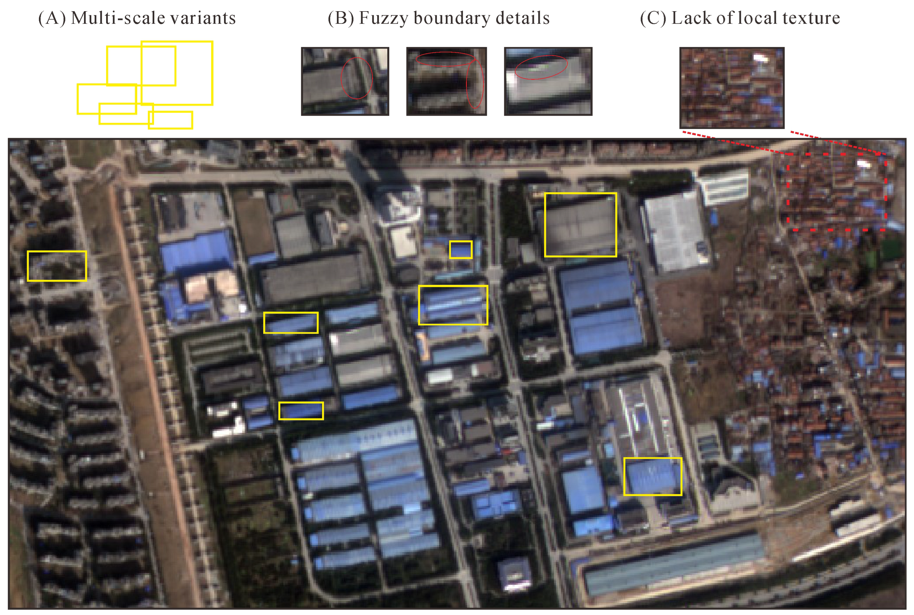
Figure 1. The main challenges of building segmentation in the LR remote-sensing imagery. (A) multi-scale variants. (B) fuzzy boundary details. (C) lack of local textures. The image was captured by the Gaofen-2 satellite with a resolution of 4 m/pixel. Red circles in subfigure (B) indicate the notable parts of the fuzzy boundary.
Remotesensing 15 01741 g001
Figure 2. Real-world examples of the SOTA method. From top to bottom, the resolution of the images are 0.3, 4, and 8 m/pixel, respectively. The circle in the upper right of the images indicates the Intersect Over Union (IoU) score (%) for buildings. (A) Image. (B) Unet++. (C) EPUNet. (D) CBR-Net.
Remotesensing 15 01741 g002
Figure 3. Schematic diagram of three types of feature fusion structures. (A) The FPN, where the top feature is directly propagated by the addition function. (B) The recent feature fusion structure with a dense affinity function, where the top feature is propagated by calculating the affinity on two adjacent layers. (C) The sparse affinity function, which only calculates the affinity of representative features.
Remotesensing 15 01741 g003
Figure 4. Frameworks of the proposed SGFANet. (A) The overall pipeline of the proposed SGFANet includes a bottom-up basic hierarchical feature extractor, a top-down feature fusion path composed of SBSM, GFM, and GT, and a decoder. (B) The sparse boundary fragment sampler module (SBSM) serves to sample the top-N representative feature points about the building boundaries (i.e., the edges and corners). N is a hyperparameter and can be different for edges and corners. (C) The gated fusion module (GFM), which is used to calculate the affinity of the selected point-wise features.
Remotesensing 15 01741 g004
Figure 5. The detailed structure of (A) the gated operator and (B) dual region propagation. The input of our gated operator is with dimension of C × N . SGFANet utilizes it in three features, e.g., D l ( p ) , D l 1 ( p ) and V i ( p ) . The dual region propagation is a kind of self-attention mechanism, for projecting the feature D l i ( p ) and E l 1 i ( p ) to one-feature embedding.
Remotesensing 15 01741 g005
Figure 6. The impact of the GT can be better recognized by a heat map of the predicted score. The building predicted scores are the output of the sigmoid layer with the range [0, 1]. (A,B) The image and the corresponding label, respectively. (C) Heatmap obtained by visualizing the values of the difference between the prediction score of SGFANet and that of SGFANet without GT.
Remotesensing 15 01741 g006
Figure 7. Statistical results of the single building size in the INRIA building dataset, including five cities, e.g., Vienna, Tyrol, Kitsap, Chicago, and Austin.
Remotesensing 15 01741 g007
Figure 8. Distributions of images and the corresponding ground truths in the proposed experiment.
Remotesensing 15 01741 g008
Figure 9. Examples of the building extraction results of the proposed SGFANet and other SOTA methods. The red squares indicate our notable improvement.
Remotesensing 15 01741 g009
Figure 10. Example of the poor extraction result. (A) Image. (B) The ground truth. (C) CBR-Net. (D) SGFANet. A distinct area of inadequate extraction is highlighted by a red circle.
Remotesensing 15 01741 g010
Figure 11. Sample images and results where the buildings are densely distributed. (A) Image tile. (B) Ground truth. (C) EPUNet. (D) SGFANet. EPUNet propagates all features of the building boundary without filtering, which limits the performance in LR imagery due to the fuzzy boundary details—particularly for the buildings in dense areas. The red squares indicate our notable improvement.
Remotesensing 15 01741 g011
Figure 12. Examples of the ability to capture building shapes. From left to right are (A) Image tile. (B) Ground truth. (C) ASLNet. (D) GFANet. ASLNet was proposed to find the regularized shape of buildings. However, it failed to predict accurate building boundaries compared with our method. The red squares indicate our notable improvement.
Remotesensing 15 01741 g012
Figure 13. Examples of the super resolution and then semantic segmentation results obtained by the different methods in Sentinel-2 images. (A) The image tile (10 m/pixel). (BD) The building extraction results (2.5 m/pixel) from ESPC_NASUnet, FSRSS-Net, and our SGFANet under the SR-then-SS framework, respectively. For better visual effects, we used the 2.5 m image from Esri community as the base map. The red squares indicate our notable improvement.
Remotesensing 15 01741 g013
Figure 14. Speed versus accuracy on the DREAM-A+ dataset. The radii of circles represent the number of parameters (million). All the methods were tested with one V-100 GPU for a fair comparison.
Remotesensing 15 01741 g014
Figure 15. The IoU on DREAM-A+ v a l of different combinations of sampled edges ( N e ) and corners ( N c ) under different strategies. First, we sampled the edge points while N c remained zero (shown in (A)). Then, based on the best N e , we sampled the corner (shown in (B)). The best combination was 192 and 8 for N e and N c , respectively. Second, we sampled the corners (shown in (C)) and then sampled the edges (shown in (D)), and the best combination was 128 and 16. Third, we kept the ratio of N e and N c to 4:1, and the best combination was 128 and 32 as shown in (E).
Remotesensing 15 01741 g015
Figure 16. Visualization of the locations of sampled points. (A) Edge points. (B) Corner points.
Remotesensing 15 01741 g016
Figure 17. Dynamic building-change-tracking results (2016–2021) of the Xiong’an New area in China. The subplots (AC) are three detail examples to show the building dynamic.
Remotesensing 15 01741 g017
Table 1. Number of image tiles in the train set, validation set, and test set for each dataset.
TrainValidationTest
DREAM-A+ dataset19507801169
Spacenet7 dataset657126283941
Sentinel-2 dataset15,27461099164
Table 2. Comparison with the related results on the benchmark. The bold values in each column means the best entries.
IoU (%)OA (%)F1 (%)b-F1 (3PX)
DeepLabV3+45.0989.2962.1563.70
Unet++46.1289.3263.1365.87
ICTNet46.6989.3263.6666.89
CBR-Net47.8089.8564.6866.73
PFNet47.2689.7264.1964.92
EPUNet45.8489.1462.8765.45
ASLNet40.4788.7958.2960.18
SGFANet48.4690.0665.2866.94
Table 3. Comparison with the related results based on the SR-then-SS framework. The bold values in each column means the best entries.
SR ModuleIoU (%)OA (%)F1 (%)
DeepLabV3+ESPCN31.0782.9047.41
Unet++ESPCN32.0483.5748.53
ICTNetESPCN32.1982.7548.71
CBR-NetESPCN32.7283.0949.53
PFNetESPCN29.4484.1145.49
EPUNetESPCN31.8383.0748.29
ASLNetESPCN28.1282.5643.90
SGFANet (ours)ESPCN33.1184.0049.75
ESPC_NASUnetESPCN30.3782.5146.59
FSRSS-Net-27.2883.6642.87
Table 4. Comparisons on DREAM-A+ of different N e and N c adjusting strategies. The bold values in each column means the best entries.
IoU (%)OA (%)F1 (%)Time (h)
SGFANet-S1
(192, 8)
51.9478.8068.5436
SGFANet-S2
(128, 16)
51.7278.5268.0436
SGFANet-S3
(128, 32)
51.8878.7068.3219
Table 5. Ablation experimental results. The bold values in each column means the best entries.
+PPM+SBSM+GFM+GTIoU (%)OA (%)F1 (%)Description
----48.4478.0762.91The baseline of the ablation studies
---48.7078.3565.50Add PPM to the top layer in the top-down procedure, the propagation is feature-wise
--49.6878.6866.38Append GT and PPM into the top-down procedure, the propagation is feature-wise
-50.3178.6966.94Append GT and PPM into the top-down procedure, the propagation is point-wise realized by the SBSM
-51.2179.1367.74Append GFM and PPM into the top-down procedure, the further contexts filtering is included in the point-wise propagation
51.8878.7068.32Our method
Table 6. Boundary F1 score. The bold values in each column means the best entries.
IoUb-F1 (3px)b-F1 (9px)b-F1 (12px)
baseline + PPM48.7055.3777.1979.65
+GT49.6855.6376.8379.29
+GT + SBSM50.3156.3377.7380.18
+GT + SBSM + GFM51.8860.4481.1383.38
Table 7. Correlation coefficients ( R 2 ) between our results and other thematic related products.
ResolutionCorrelation Coefficients
Dynamic World10 m0.7702
GAIA30 m0.6864
MCD12Q1500 m0.4907
Disclaimer/Publisher’s Note: The statements, opinions and data contained in all publications are solely those of the individual author(s) and contributor(s) and not of MDPI and/or the editor(s). MDPI and/or the editor(s) disclaim responsibility for any injury to people or property resulting from any ideas, methods, instructions or products referred to in the content.