Article

Machine Learning Models for Approximating Downward Short-Wave Radiation Flux over the Ocean from All-Sky Optical Imagery Based on DASIO Dataset

1
Shirshov Institute of Oceanology, Russian Academy of Sciences, 36 Nakhimovskiy pr., Moscow 117997, Russia
2
Moscow Institute of Physics and Technology, 9 Institutskiy per., Dolgoprudny 141701, Russia
3
Moscow Center for Fundamental and Applied Mathematics, Moscow 119991, Russia
*
Author to whom correspondence should be addressed.
Remote Sens. 2023, 15(7), 1720; https://doi.org/10.3390/rs15071720
Submission received: 3 January 2023 / Revised: 2 March 2023 / Accepted: 20 March 2023 / Published: 23 March 2023
(This article belongs to the Special Issue Remote Sensing of the Earth’s Radiation Budget)

Abstract

:
Downward short-wave (SW) solar radiation is the only essential energy source powering the atmospheric dynamics, ocean dynamics, biochemical processes, and so forth on our planet. Clouds are the main factor limiting the SW flux over the land and the Ocean. For the accurate meteorological measurements of the SW flux one needs expensive equipment-pyranometers. For some cases where one does not need golden-standard quality of measurements, we propose estimating incoming SW radiation flux using all-sky optical RGB imagery which is assumed to incapsulate the whole information about the downward SW flux. We used DASIO all-sky imagery dataset with corresponding SW downward radiation flux measurements registered by an accurate pyranometer. The dataset has been collected in various regions of the World Ocean during several marine campaigns from 2014 to 2021, and it will be updated. We demonstrate the capabilities of several machine learning models in this problem, namely multilinear regression, Random Forests, Gradient Boosting and convolutional neural networks (CNN). We also applied the inverse target frequency (ITF) re-weighting of the training subset in an attempt of improving the SW flux approximation quality. We found that the CNN is capable of approximating downward SW solar radiation with higher accuracy compared to existing empiric parameterizations and known algorithms based on machine learning methods for estimating downward SW flux using remote sensing (MODIS) imagery. The estimates of downward SW radiation flux using all-sky imagery may be of particular use in case of the need for the fast radiative budgets assessment of a site.

1. Introduction

Solar radiation is the main source of energy on Earth [1]. It is also of great significance for biogeochemical, physical, ecological, and hydrological processes [2,3]. Cloud cover, in turn, is the main physical factor limiting the downward solar radiation flux [4,5,6]. Cloud cover during the day reduces the influx of solar radiation to the Earth’s surface, and significantly weakens its outgoing long-wave radiation at night due to backscattering [7]. This entails corresponding changes in other meteorological quantities. The functioning of agriculture, transport, aviation, resorts, alternative energy enterprises, and other sectors of the economy, in one way or another, depends on the amount and shape of clouds.
There are two options for flux estimation in modern models of climate and weather forecasts. The first is physics-based modeling of radiation transfer through two-phase medium (clouds), which includes modeling of multi-scattering, taking into account the microphysics of cloud water drops [8] and aerosols. This option is extremely computationally expensive. Alternatively, one may use parameterizations which are simplified schemes for approximating environmental variables using only routinely observed cloud properties, such as Total Cloud Cover (TCC), cloud types, and cloud cover per height layer. The existing parametrizations are empirical and were proposed years and decades ago based on observations and expert-based assumptions [9,10]. As a result, they may not take into account the entire variety of cloud situations occurring in nature, which may lead to a reduced quality of approximation of downward SW solar radiation flux.
Our goals were to get computationally cheaper estimations of downward solar radiation flux and to study flux dependence on structural characteristics of clouds. The aim of this study was to improve the accuracy of existing parameterizations of downward SW radiation flux. In this study, we assess the capability of machine learning models in the scenario of statistical approximation of radiation flux from all-sky optical imagery. We solve the problem using various machine learning (ML) models with the assumption that an all-sky photo contains complete information about the downward SW radiation.
There are a number of studies on the forecasting of downward SW radiation using advanced statistical models, namely, machine learning models [3,11,12]. Most of them deal with the time-series of SW radiation flux measured directly by an instrument (radiometer); thus, in case of the need for a low-cost assessment package, one cannot apply this approach. There are also a number of ML methods published for estimating other useful properties of the clouds, for example, total cloud cover [13,14] or cloud types [15,16,17].
There are a number of studies demonstrating the capabilities of machine learning methods in estimating the SW flux from remote sensing data, for example, MODIS [3,18] or GMS-5 [19]. There are also studies demonstrating the links between properties of cloud cover and surface solar irradiance [20,21]. However, these studies are not focused on approximating the flux directly from all-sky imagery. Rather, in these studies, all-sky imagery is commonly used for assessing some semantically meaningful properties of cloud cover, that are then used to categorize the events of solar irradiance measurements.
To the best of our knowledge, there is only one study demonstrating the capabilities of statistical modeling in the problem of the estimation of downward SW radiation flux [22]. In this study, though, the statistical relation is demonstrated between the semantically rich meteorological features (solar zenith angle, surface albedo, hemispherical effective cloud fraction, ground altitude and atmospheric visibility) and the SW radiation flux. In contrast with this study, we model the statistical relations between the raw all-sky imagery and the SW radiation flux. We do not propose to infer any of semantically significant features of the all-sky visual scene. The only semantically meaningful feature we propose to use is the sun altitude, which we compute using the position, date, and time of observations.
The rest of the paper is organized as follows: in Section 2, we describe the dataset that we used in our study; in Section 3, we introduce the methods we exploited in our study for approximating the SW downward radiation flux; in Section 4, we present and discuss the results of our study. In Section 6, we summarize the paper and present the outlook for further study.

2. Data

In this section, we present source data for our study. The problem we tackle is to map all-sky imagery to net downward SW radiation flux using state-of-the-art statistical models (also known as machine learning models). We used a high-resolution fish-eye cloud-camera «SAIL cloud v.2» [14], also known as SAILCOP (which stands for “Sea–Air Interactions Laboratory Clouds Optical Package”) [13] to collect all-sky images, and a Kipp and Zonen CNR-1 net radiometer (Kipp and Zonen, Delft, The Netherlands) to measure net downward SW flux. In Figure 1, we present the equipment used to collect the data.
The net radiometer Kipp and Zonen CNR-1 is a tool used for the measurements of incoming and outgoing net solar (also known as short-wave, SW hereafter) and far-infrared (also known as long-wave, LW hereafter) radiation in various weather conditions, including rough seas. The CNR-1 net radiometer is equipped with four separate sensors: two for downward fluxes (SW and LW components), and the rest for outgoing radiation (SW and LW components). The CNR-1 design is such that both the upward-facing and downward-facing sensors measure the energy that is received from the whole hemispheres, upper and lower, thus having a 180-degree field of view. The output is expressed in Watts per square meter; thus, one may use the measurements as is, without any transformations. The spectral range covers both the SW radiation, meaning wavelengths from 300 to 3000 nm, and the LW radiation, meaning wavelengths from 4.5 to 42 μ m. SW net radiation is measured by two pyranometers, one for measuring incoming radiation from the sky, and the other, which faces downward, for measuring the reflected SW radiation. LW radiation is measured by two pyrgeometers, one for measuring the LW radiation from the sky, and the other from the sea surface. We use the CNR-1 net radiometer in the four Separate Components Mode (4SCM) [23]. According to the user manual [23], the nonlinearity of the measurements of both SW and LW sensors is ± 2.5 % . In recent studies, the CNR-1 net radiometers were compared to high-standard reference radiation instruments measuring individual SW and LW downward and upward flux components [24]. It was shown that the CNR-1 radiometer demonstrates quite a high measurement quality commonly characterized by root-mean-square errors below 14 Wm 2 . In our study, we used the measurements as is, without any corrections. In our marine missions, though, the CNR-1 net radiometer was mounted close to the shipboard; thus, the reflected SW and LW radiation was strongly influenced by the reflection and self-irradiance of the board. Thus, we did not use the outgoing radiation measurements.
The fish-eye cloud-camera SAILCOP is developed and assembled in Sea-Air Interactions Laboratory, Shirshov Institute of Oceanology, Russian Academy of Sciences, Moscow, Russia. It was first presented in 2016 [14]. It was designed following the concept of all-sky digital optical imagers presented in 1998 by Long et al. [25]. The concept was then adopted in various recent studies [26,27,28,29,30,31,32,33,34]. The term “cloud-camera”, which we use here, is a synonym for “all-sky camera”, “all-sky imager”, “whole sky camera”, “total sky imager”, and many others similar to those mentioned in the studies referenced above. The main function of these packages is to register the visual image of the visible hemisphere of the sky-dome using a ground-based optical fish-eye camera. In our marine expeditions, our all-sky camera was mounted onboard a ship, and directed upwards when the ship was not waving. An all-sky camera commonly has a 180-degree field of view; thus, an image taken by it presents the whole visible part of the sky. The common purpose of an all-sky imager is to register the sky with visible clouds in order to automatically retrieve properties of clouds that are historically assessed by a human observer, for example, total cloud cover [13,31,34] or cloud types [17,35,36,37,38,39]. In our optical package, we used an all-sky fish-eye optical camera, Vivotek FE8171V [40,41]. One may examine its complete characteristics in the Data Sheet [41] or User’s Manual [40]. Here, we emphasize its main properties in Table 1. The camera was operated by a software package developed in our Sea–Air Interactions Laboratory of the Shirshov Institute of Oceanology, Russian Academy of Science. The software runs on a personal computer collecting the imagery and concurrent data. The concurrent data were acquired by an extra mini-computer equipped with a GPS device and a positioning sensor (see the box under the camera in Figure 1b). The concurrent data include NMEA sentences from the GPS device, 50 Hz three-dimensional accelerometer measurements, 50 Hz three-dimensional gyroscope measurements, and additional service readings. The software on the operating personal computer requests imagery from the optical camera once during a 10-s period if the camera is horizontal according to the accelerometer. The communication of an operating personal computer with the camera and mini-computer was established using a high-speed TCP/IP connection over an Ethernet cable, which was also used to provide a power supply to both the camera and the mini-computer using PoE (Power over Ethernet) technology. SAILCOP includes two identical optical cameras, each equipped with its own extra mini-computer, GPS device, and positioning sensor. We mounted them apart from each other and measured the distance between them. The software on the operating personal computer requests imagery from both optical cameras simultaneously. This way, we always acquire two images of the same sky-dome taken from two different points 15 to 35 m apart, depending on the ship and mounting scheme.
Due to a common misconception that can be observed during various discussions about all-sky imagery, we describe here the sense of all-sky images. They are the hemispheric photographs of the upper visible hemisphere taken from the ground, from the sea surface, or from the board of a ship using a fish-eye optical camera directed upwards, or employing a hemispherical mirror with a narrow-angle camera [25] (see an example of an all-sky image in Figure 1c). In an all-sky image, one may usually observe the blue sky partially covered with (commonly) white clouds of various degrees of translucency. An all-sky camera is commonly used to assess cloud features; thus, it is usually mounted apart from large structures in order to prevent them from obscuring a substantial fraction of a visible sky-dome. In the case of marine expeditions, one cannot place the cameras far enough from high structures of the ship; thus, we use a mask covering the parts of the ship in an image (see black regions in Figure 1c).
The source data we used in our study was the Dataset of All-sky Imagery over the Ocean (DASIO) [13], which we collected in marine expeditions starting from 2014 using the equipment we presented above. The regions covered in these missions include the Indian and Atlantic oceans, Mediterranean sea, and Arctic ocean. In this dataset, the exhaustive set of cloud types is present. DASIO contains over 1,500,000 images of the sky-dome over the ocean, accompanied by downward SW radiation flux measurements. SW solar flux was averaged over 10 s intervals, and the all-sky images were registered every 20 s. The viewing angle of the Kipp&Zonen CNR-1 sensors was 180° in both vertical planes. The viewing angle of the cloud-camera was similar. Photos taken from the fisheye cloud-camera had a high enough resolution to resolve fine cloud structural details (1920 × 1920 px). The white balance and brightness of photos was adjusted automatically for the most comfortable visual experience.
In our study, we employed a subset of DASIO. The size of the training subset was more than 1,000,000, and the size of the test subset was more than 350,000 images (see Table 2). In other words, the ratio of the volumes of test and training subsets is 1:3. A particular sampling strategy was involved when we split the dataset into training and testing subsets. Since the period of image acquisition is 20 s, the visual scene of the sky-dome does not change substantially between subsequent images. Thus, two subsequent all-sky images are strongly correlated. In this case, subsequent images may be considered identical with small perturbations. Since training and testing subsets should not include identical examples, one needs to sample subsequent images in such a way that it prevents images from falling into training and test sets on a systematic basis. The issue of strongly correlated examples being massively included into training and testing subsets may arise in the case of random per-image sampling. In order to avoid this issue, we applied temporal block-folded sampling. To be precise, we applied random sampling using hours of observations instead of objects (images) themselves.
In the ML approach, one also needs to split the dataset into training and testing subsets in a way that would preserve the statistical characteristics in both of them. In the case of the sampling strategy we exploited in our study, our training and testing subsets have the same statistical characteristics. In order to demonstrate this, we present the distributions of target value (SW flux) in Figure 2b for both training and testing subsets. One may clearly see that the distributions are close to each other.
In Figure 3, we present the map of the missions that were included in the DASIO subset we employed in this study. One may observe that the tracks of the missions are not continuous, since we limited the set of examples based on local sun elevation; that is, we excluded the examples of the DASIO dataset with a sun elevation lower than 5 . Thus, during the nighttime, there were no data. In Table 3, we also provide a brief summary of the research missions contributing to the DASIO subset used in this study.
Figure 1c also demonstrates a mask we applied to each photo, which filters out visual objects that are not related to the subject of our study. In addition, when training our ML models, we used only the data acquired during daylight hours. In particular, we subset the images taken when the sun altitude exceeded 5 , and the radiation flux exceeded 5 W/m 2 .
We state the problem as follows: for each observation of the whole sky registered in an all-sky image, one needs to approximate the value of the short-wave radiation flux, which is supervised in the form of CNR-1 measurements. In terms of the machine learning (ML) approach, it is a regression task with the scalar target value. We used mean squared error as a loss function for the ML models exploited in this study. We also characterized the quality of the solutions using a mean absolute error (MAE) measure.

Inverse Target-Frequency (ITF) Re-Weighting of Training Subset

In target value distribution (see Figure 4), one may notice a strong predominance of data points with low SW flux. Thus, the dataset is strongly imbalanced w.r.t. target value. This kind of issue may cause reduced approximation quality [42,43]. In our study, we chose to exploit the approach of weighting the data space (following the terminology of [43]). In order to improve the approximation skills of our models, we balanced the training dataset using inverse-frequency re-weighting. We named it inverse target frequency (ITF) re-weighting. To be precise, we made the weights w i of individual examples of the training dataset inversely proportional to the frequency of target values:
w i = d i · N p i = 1 N p d i d i ,
where i enumerates inter-percentile intervals from 0-th to 99-th; d i are the inter-percentile intervals of empiric target value distribution, and N p = 100 is a number of inter-percentile intervals. Here, the less the target frequency, the greater the inter-percentile interval d i ; thus, the greater the weights w i of the examples. In order to illustrate the approach we propose, we present percentile-wise vertical lines in Figure 4, so one may notice uneven inter-percentile distances in the cumulative distribution function figure.
In addition to the ITF re-weighting, we also propose the scheme for controlling the re-weighting strength using the α coefficient:
w i = ( w i 1 ) · α + 1 .
Here, one may notice that the closer the α gets to 1, the stronger the re-weighting which is applied. In the case where α = 0 , there is no re-weighting, meaning w i = 1 . Given the form of the weights w i and w i , one may notice that their expected value is exactly 1.0 . Coefficient α is a hyperparameter of our re-weighting scheme, which is optimized during the hyperparameter optimization stage.
In order to demonstrate the effect of ITF re-weighting, we present the resulting histogram in Figure 2a. In this histogram, we show the frequencies for inter-percentile ranges of target value (SW flux) scaled in accordance with the ITF re-weighting scheme. One may notice that the bars of the histogram have uneven widths. This is expected behavior, since we demonstrate the resulting distribution for the set of inter-percentile intervals that are uneven (see Figure 4b). One may clearly see that the effective frequencies of various inter-percentile ranges are close to each other. Thus, one may consider the dataset balanced w.r.t. target value.

3. Methods

3.1. Feature Engineering

An arbitrary optical digital image may be considered an array of size W × H × C , where W and H are its width and height in pixels, and C is the channel number, C = 3 for a regular RGB image. Here, RGB stands for red, green and blue components of the color of a pixel in the RGB color model [44]. When composing the feature space for an image, we collected various statistics of each color channel (R,G,B) excluding masked pixels. A mask is the black-and-white binary picture obscuring constructions of a ship visible in an all-sky image. These constructions are irrelevant in our problem. One may observe an example of a mask (black part of the image) in Figure 1c. Here, we enlist the statistics we collect for each color channel of all-sky images as real-valued features of feature space:
  • Maximum and minimum values;
  • Sample mean;
  • Sample variance;
  • Sample skewness;
  • Sample kurtosis;
  • Sample estimates of the following percentiles: p 1 , p 5 , p 10 , p 15 , p 20 , … , p 90 , p 95 , p 99 (21 in total). Here, p d stands for a sample estimate of the percentile of level d.
There are various color models [44], including one that is particularly useful in cloud detection when using optical imagery, which is a HSV color model. Here, H, S, and V stand for Hue, Saturation, and Value. The latter is strongly correlated with brightness and intensity calculated in other color models. Since these characteristics of pixels are useful in cloud detection, segmentation, and classification problems [32,45], we decided to include the same statistics (see the list above) of HSV channels into feature space as well. Additionally, since downward SW radiation flux is strongly dependent on the sun altitude [9], we included this feature into feature space.
Using the statistics types listed above (27 in total including 21 percentiles) computed for all of the six color channels (R,G,B,H,S,V), as well as sun elevation, we engineered a 163-dimensional real-valued feature space for all-sky images in our study. The feature engineering step was only performed when we employed classic machine learning models (see Section 3.2).

3.2. Machine Learning Methods

In our study, we used two approaches: the classic approach, and the so-called end-to-end approach with the convolutional neural network employed.

3.2.1. Classic Models

Within the classic approach, we examined the following ML models: multilinear regression and non-parametric ensemble models, that is, Random Forests (RF) [46] and Gradient Boosting (GB) [47,48,49]. Training and inference of the “classical” ML models in our study was performed using scikit-learn [50] implementations of these models.

3.2.2. Convolutional Neural Network
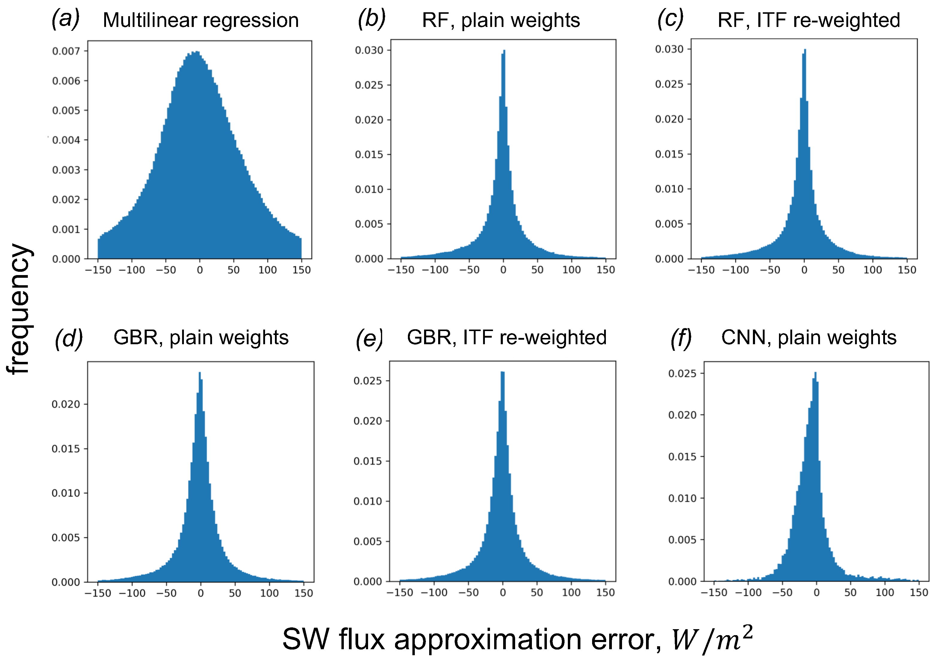
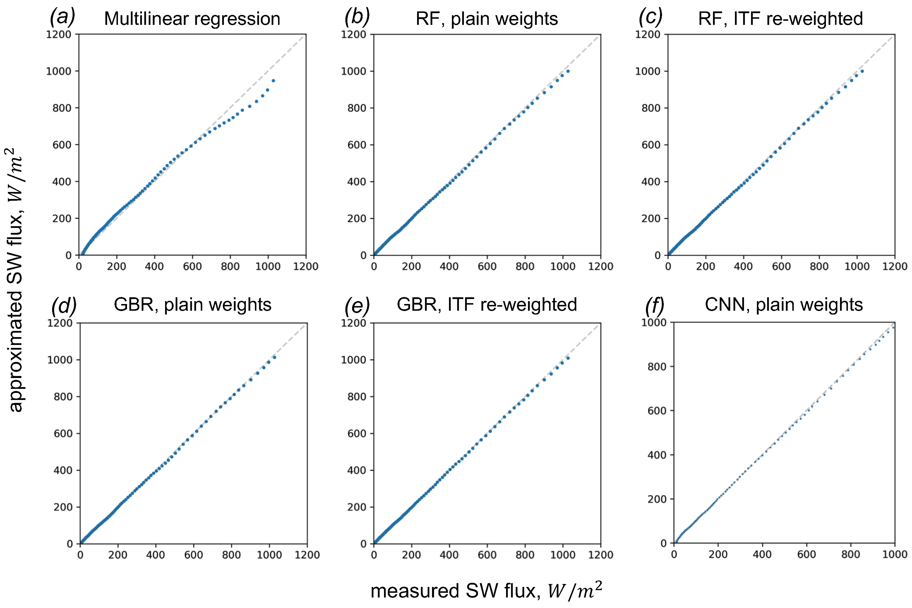
Within the end-to-end approach, we did not compute any of the expert-designed features described in Section 3.1. In contrast, we applied a convolutional neural network (CNN) [51] directly to the images.
Prior to the processing of an image by our CNN, we preprocessed the image. First, we resized the image to 512 × 512 px size using the “nearest neighbor” aggregation method. Then, we applied strong alterations of average brightness. We altered the brightness in order to encourage the CNN to learn the dependency of SW flux on the cloud spatial structure, rather than average brightness, average blue saturation, or other simple statistics of the image. We also added spatially correlated Gaussian noise to each image in order to prevent CNN from learning the dependency of SW flux on channels’ simple aggregated statistics (e.g., mean, variance). These augmentations are also meant to increase the generalization ability of our CNN. Within this end-to-end neural networks-based approach, we used the feature of sun altitude, as well as in the case of classic machine learning models.
The structure of the CNN exploited in our study is shown in Figure 5. As one may see in this figure, the input example is an all-sky RGB image resized to the resolution of 512 × 512 px. In order to speed up the training process and improve the quality of the approximation, we employed the transfer learning approach [52]. That is, a pre-trained version of ResNet50 [53] network was used, which was pre-trained on the ImageNet [54] dataset. The output of the ResNet50 convolutional sub-network is a 2048-dimensional vector. We concatenated the sun altitude to this vector; thus, the resulting vector is 2049-dimensional. This 2049-dimensional vector is then processed by a fully connected sub-network. The structure of this sub-network is presented in Figure 5. The output of this subnet is a real scalar value approximating SW flux.
When training our CNN, we used the Adam stochastic optimization algorithm [55]. Training and inference of our CNN was implemented with a Python programming language [56] using Pytorch [57], OpenCV [58] for Python, and other high-level computational libraries for Python.
In both the ensemble models (RF and GB) we exploited in our study, there are hyperparameters besides the α re-weighting coefficient we presented above. Among them are the ensemble members in RF and GB, the maximum depth of the trees of the ensemble, and so forth. The CNN is also characterized by a number of hyperparameters: its depth, the width of fully connected layers in fully connected subnets, the hyperparameters of the Adam optimization procedure, and also the magnitude of data augmentation transformations. We employed the Optuna framework [59] for hyperparameter optimization (HPO). During the HPO stage, the quality of each model initialized with a sampled hyperparameter set is assessed within the K-fold cross-validation (CV) approach with K = 5 . Due to strongly correlated examples (all-sky images) that are close in temporal domain, we ensured the independence of training and validation CV subsets using a Group K-fold cross-validation approach where groups are hourly subsets of all-sky images. In the case of RF and GB models, we assessed the mean RMSE measure, as well as its uncertainty within the Group K-fold CV approach.

4. Results

In this section, we present the results of our study. To assess the quality of our models, we used the root mean square error (RMSE) measure. In order to estimate the uncertainty of the quality measures, we trained and evaluated each model several times (typically, 5–7) and estimated the confidence interval of 95% significance levels, assuming the RMSE is a normally distributed random variable. Additionally, the visual representation of the results is given in the form of value mapping diagrams (Figure 6), where the correspondence between approximated and measured flux values is presented in the form of point density. In Figure 7, we present the error histograms for the models involved in our study.
In Figure 6 and Figure 8, one may see that the models generally underestimate high fluxes and overestimate low fluxes. It is also clear that the multilinear model approximates the flux worse than other models, which is supported by the RMSE measures in Table 4 and quantile–quantile plots in Figure 8. The results of CNN are the best among others in terms of formal RMSE measures, as well as approximated-to-measured value-mapping diagrams.
In our study, we built and trained four ML models to approximate the downward shortwave radiation flux. We found that the quality of the CNN, which was built within the end-to-end approach, is the best compared to other ML models. As we mentioned in Section 1, there are no previously published papers demonstrating any methods for approximating downward SW flux using all-sky imagery. Thus, the only approaches we may compare with are the ones that propose estimating downward SW flux using complementary data (e.g., geoposition, date and time, properties of clouds) also known as parameterizations. In this study, we compared the quality of our models with existing SW radiation parameterizations known from the literature [9,10] and existing algorithms based on machine learning for estimating downward SW flux using remote sensing (MODIS) imagery [3]. In Table 4, we presented the quality of our models assessed after the hyperparameter optimization. We also provided RMSE estimates of the parametrizations [9,10] and an ML-based algorithm applied on MODIS imagery [3] as a reference. One may observe that parameterization errors strongly depend on the amount of cloudiness: the higher the total cloud cover (TCC), the higher a parameterization error. We have provided the error range in brackets for parameterizations known from the literature.
In Figure 7, we also demonstrate error distributions for each of the ML models of our study. In the CNN error distribution (Figure 7d), one may see that the neural network is prone to underestimate the SW flux slightly. Additionally, it is clear that error distribution tails are pretty heavy for both the RF and GB models, and are light for CNN. These features of error distribution for our models are also in agreement with the variance of errors that have been presented in Table 4 in the form of RMSE (taking into account that the errors are zero-centered; thus, RMSE is the square root of variance in this case).

5. Discussion

One may observe that the ITF re-weighting did not make any difference in terms of the RMSE quality measure. Neither Random Forests, nor Gradient Boosting for Regression models demonstrated any performance improvement due to ITF re-weighting. It is a common belief in the machine learning community that in order to improve the performance of a ML model in a problem characterized by a strongly imbalanced dataset, one needs to re-weight it, bringing the distribution of target variables close to uniform distribution. Alternatively, one needs to apply a sampling strategy that has an equivalent effect in the case of mini-batch training, such as when training artificial neural networks. In this study, we applied proper re-weighting that brings the effective distribution of downward SW flux to a uniform distribution. We present here the results of machine learning models with ITF re-weighting applied in order to demonstrate a perfect case of a strongly imbalanced dataset where a proper hyperparameter-optimized re-weighting does not improve ML models’ performance.
One may also note that the models we present demonstrate some issues. Multilinear regression is a fast model; however, it has the worst quality. RF and GBR demonstrate comparable quality and are relatively fast in their inference times. At the same time, one may note non-smooth error distribution in diagrams in Figure 6b–e. We suppose that the regular drops in point density may be explained by the decision-tree-based nature of these two ensemble models. One may also notice the outliers in these diagrams that may be of interest in forthcoming studies. In this study, we did not filter the outliers comprehensively; thus, there may be irrelevant examples in the dataset that represent photographs of birds, operators cleaning the glass dome of SAILCOP cameras, and so forth.
There are limitations to the approach we used in our study for approximating downward SW flux from all-sky RGB optical imagery. We found that our CNN is capable of approximating SW flux by relying on the spatial structure of clouds present in an all-sky image. We even encouraged our CNN to learn this link by applying heavy image augmentations described in Section 3.2. However, in the presence of fog or haze, it is most probable that most clouds will be present in a corresponding all-sky image; thus, the method exploiting our CNN may deliver SW flux estimates with certain errors. The degree of uncertainty imposed by particular meteorological conditions, including the presence of fog, haze, and strong aerosol pollution, is to be assessed in forthcoming studies.

6. Conclusions

In this study, we presented an approach for the approximation of short-wave solar radiation flux over the ocean from all-sky optical imagery using state-of-the-art machine learning algorithms, including multilinear regression, Random Forest, Gradient Boosting, and Convolutional Neural Networks. We trained our models using the data of the DASIO dataset [13]. We assessed the quality of our models in terms of root mean squared error (RMSE), approximated versus measured flux diagrams, error histograms, and quantile–quantile plots. The results allowed us to conclude that one may estimate downward SW radiation flux directly from all-sky imagery, taking some well-known uncertainty into account. We also demonstrate that our CNN trained with strong data augmentations is capable of estimating downward SW radiation flux, mostly based on clouds’ visible structure. At the same time, the CNN has shown to be superior in terms of flux RMSE compared to other ML models in our study.
Our method of flux estimation may be especially useful in the tasks of low-cost monitoring of downward SW flux. From a practical point of view, one may use an all-sky imager instead of high-grade radiometer in order to assess the radiative regimen of a region using a low-cost, all-sky camera. In our study, we demonstrated that a low-cost optical package accompanied by a trained ML algorithm may provide SW flux estimates of reasonable quality. These estimates may be useful for planning the positions of solar power plants, predicting the power plants generation, and so forth.
In our study, we demonstrated that the SW flux may be estimated by a ML model with a reasonable quality using all-sky imagery and sun elevation only. At the same time, there are a number of studies presenting the methods for retrieving various cloud properties from all-sky images [13,14,16,25,37,38,39]. Thus, one may use these methods for assessing the properties of clouds and downward SW radiation based on an all-sky image, and hence, train an ML model linking the properties of clouds to SW radiation flux. One may also assess the same cloud properties from atmospheric models. Thus, there is a way to use an ML model to estimate downward SW flux based on modeled atmospheric data containing characteristics of clouds. This method of estimating SW flux in an atmospheric model may significantly reduce the computational load of its radiation subroutine.
Our results suggest that there are outliers in the DASIO dataset that may be filtered in forthcoming studies. The results also suggest that hyperparameter optimization of our CNN and ensemble models may help in discovering better configurations, including proper dataset re-weighting, as well as more suitable CNN architecture.
In further studies, we plan to improve the approach of resampling and re-weighting. We also plan to approximate downward long-wave solar radiation flux using an approach similar to the one presented in this paper. Additionally, modern statistical models of the machine learning class provide an opportunity for short-term forecasting of fluxes, which may be useful in forecasting the generation of solar power plants.

Author Contributions

Conceptualization, M.K. and S.G.; data curation, V.K., N.A. and S.G.; funding acquisition, S.G.; methodology, M.K.; project administration, M.A.; software, M.K., V.K., M.B. and N.A.; supervision, S.G.; validation, V.K., M.B. and N.A.; writing—original draft, M.K. and V.K.; writing—review & editing, M.K. and M.A. All authors have read and agreed to the published version of the manuscript.

Funding

This research was supported by an Agreement with the Ministry of Science and Higher Education No. 13.2251.21.0120 (unique identifier RF-2251.61321X0014, 075-15-2021-1398).

Data Availability Statement

Publicly available datasets were analyzed in this study. This data can be found here: https://dasio.ru/.

Conflicts of Interest

The authors declare no conflict of interest.

Abbreviations

The following abbreviations are used in this manuscript:
CNNConvolutional neural network
DLDeep learning
MLMachine learning
SWshort wave
LWlong wave
DASIODataset of All-Sky Imagery over the Ocean
RFRandom Forests
LRLinear regression
MLRMultilinear regression
GBRGradient Boosting for Regression

References

  1. Trenberth, K.E.; Fasullo, J.T.; Kiehl, J. Earth’s Global Energy Budget. Bull. Am. Meteorol. Soc. 2009, 90, 311–324. [Google Scholar] [CrossRef] [Green Version]
  2. Stephens, G.L.; Li, J.; Wild, M.; Clayson, C.A.; Loeb, N.; Kato, S.; L’Ecuyer, T.; Stackhouse, P.W.; Lebsock, M.; Andrews, T. An update on Earth’s energy balance in light of the latest global observations. Nat. Geosci. 2012, 5, 691–696. [Google Scholar] [CrossRef]
  3. Wu, H.; Ying, W. Benchmarking Machine Learning Algorithms for Instantaneous Net Surface Shortwave Radiation Retrieval Using Remote Sensing Data. Remote Sens. 2019, 11, 2520. [Google Scholar] [CrossRef] [Green Version]
  4. Cess, R.D.; Nemesure, S.; Dutton, E.G.; Deluisi, J.J.; Potter, G.L.; Morcrette, J.J. The Impact of Clouds on the Shortwave Radiation Budget of the Surface-Atmosphere System: Interfacing Measurements and Models. J. Clim. 1993, 6, 308–316. [Google Scholar] [CrossRef]
  5. McFarlane, S.A.; Mather, J.H.; Ackerman, T.P.; Liu, Z. Effect of clouds on the calculated vertical distribution of shortwave absorption in the tropics. J. Geophys. Res. Atmos. 2008, 113, D18203. [Google Scholar] [CrossRef] [Green Version]
  6. Lubin, D.; Vogelmann, A.M. The influence of mixed-phase clouds on surface shortwave irradiance during the Arctic spring. J. Geophys. Res. Atmos. 2011, 116, D00T05. [Google Scholar] [CrossRef] [Green Version]
  7. Chou, M.D.; Lee, K.T.; Tsay, S.C.; Fu, Q. Parameterization for Cloud long-wave Scattering for Use in Atmospheric Models. J. Clim. 1999, 12, 159–169. [Google Scholar] [CrossRef] [Green Version]
  8. Stephens, G.L. Radiation Profiles in Extended Water Clouds. I: Theory. J. Atmos. Sci. 1978, 35, 2111–2122. [Google Scholar] [CrossRef]
  9. Aleksandrova, M.; Gulev, S.; Sinitsyn, A. An improvement of parametrization of short-wave radiation at the sea surface on the basis of direct measurements in the Atlantic. Russ. Meteorol. Hydrol. 2007, 32, 245–251. [Google Scholar] [CrossRef]
  10. Dobson, F.W.; Smith, S.D. Bulk models of solar radiation at sea. Q. J. R. Meteorol. Soc. 1988, 114, 165–182. [Google Scholar] [CrossRef]
  11. Ebtehaj, I.; Soltani, K.; Amiri, A.; Faramarzi, M.; Madramootoo, C.A.; Bonakdari, H. Prognostication of Shortwave Radiation Using an Improved No-Tuned Fast Machine Learning. Sustainability 2021, 13, 8009. [Google Scholar] [CrossRef]
  12. Voyant, C.; Notton, G.; Kalogirou, S.; Nivet, M.L.; Paoli, C.; Motte, F.; Fouilloy, A. Machine learning methods for solar radiation forecasting: A review. Renew. Energy 2017, 105, 569–582. [Google Scholar] [CrossRef]
  13. Krinitskiy, M.; Aleksandrova, M.; Verezemskaya, P.; Gulev, S.; Sinitsyn, A.; Kovaleva, N.; Gavrikov, A. On the generalization ability of data-driven models in the problem of total cloud cover retrieval. Remote Sens. 2021, 13, 326. [Google Scholar] [CrossRef]
  14. Krinitskiy, M.A.; Sinitsyn, A.V. Adaptive algorithm for cloud cover estimation from all-sky images over the sea. Oceanology 2016, 56, 315–319. [Google Scholar] [CrossRef]
  15. Liu, S.; Duan, L.; Zhang, Z.; Cao, X.; Durrani, T.S. Multimodal Ground-Based Remote Sensing Cloud Classification via Learning Heterogeneous Deep Features. IEEE Trans. Geosci. Remote Sens. 2020, 58, 7790–7800. [Google Scholar] [CrossRef]
  16. Liu, S.; Li, M.; Zhang, Z.; Xiao, B.; Cao, X. Multimodal Ground-Based Cloud Classification Using Joint Fusion Convolutional Neural Network. Remote Sens. 2018, 10, 822. [Google Scholar] [CrossRef] [Green Version]
  17. Taravat, A.; Frate, F.D.; Cornaro, C.; Vergari, S. Neural Networks and Support Vector Machine Algorithms for Automatic Cloud Classification of Whole-Sky Ground-Based Images. IEEE Geosci. Remote Sens. Lett. 2015, 12, 666–670. [Google Scholar] [CrossRef]
  18. Chen, J.; He, T.; Jiang, B.; Liang, S. Estimation of all-sky all-wave daily net radiation at high latitudes from MODIS data. Remote Sens. Environ. 2020, 245, 111842. [Google Scholar] [CrossRef]
  19. Lu, N.; Liu, R.; Liu, J.; Liang, S. An algorithm for estimating downward shortwave radiation from GMS 5 visible imagery and its evaluation over China. J. Geophys. Res. Atmos. 2010, 115, 1–15. [Google Scholar] [CrossRef]
  20. Pfister, G.; McKenzie, R.; Liley, J.; Thomas, A.; Forgan, B.; Long, C.N. Cloud coverage based on all-sky imaging and its impact on surface solar irradiance. J. Appl. Meteorol. Climatol. 2003, 42, 1421–1434. [Google Scholar] [CrossRef]
  21. Tzoumanikas, P.; Nikitidou, E.; Bais, A.; Kazantzidis, A. The effect of clouds on surface solar irradiance, based on data from an all-sky imaging system. Renew. Energy 2016, 95, 314–322. [Google Scholar] [CrossRef]
  22. Chen, L.; Yan, G.; Wang, T.; Ren, H.; Calbó, J.; Zhao, J.; McKenzie, R. Estimation of surface shortwave radiation components under all sky conditions: Modeling and sensitivity analysis. Remote Sens. Environ. 2012, 123, 457–469. [Google Scholar] [CrossRef]
  23. Kipp & Zonen. CNR 1 Net Radiometer Instruction Manual. Available online: https://www.kippzonen.com/Download/85/Manual-CNR-1-Net-Radiometer-English (accessed on 27 February 2023).
  24. Michel, D.; Philipona, R.; Ruckstuhl, C.; Vogt, R.; Vuilleumier, L. Performance and Uncertainty of CNR1 Net Radiometers during a One-Year Field Comparison. J. Atmos. Ocean. Technol. 2008, 25, 442–451. [Google Scholar] [CrossRef]
  25. Long, C.; DeLuisi, J. Development of an automated hemispheric sky imager for cloud fraction retrievals. In 10th Symposium on Meteorological Observations and Instrumentation: Proceedings of the 78th AMS Annual Meeting, Phoenix, AZ, USA, 11–16 January 1998; American Meteorological Society (AMS): Boston, MA, USA, 1998; pp. 171–174. [Google Scholar]
  26. Wang, Y.; Liu, D.; Xie, W.; Yang, M.; Gao, Z.; Ling, X.; Huang, Y.; Li, C.; Liu, Y.; Xia, Y. Day and Night Clouds Detection Using a Thermal-Infrared All-Sky-View Camera. Remote Sens. 2021, 13, 1852. [Google Scholar] [CrossRef]
  27. Sunil, S.; Padmakumari, B.; Pandithurai, G.; Patil, R.D.; Naidu, C.V. Diurnal (24 h) cycle and seasonal variability of cloud fraction retrieved from a Whole Sky Imager over a complex terrain in the Western Ghats and comparison with MODIS. Atmos. Res. 2021, 248, 105180. [Google Scholar] [CrossRef]
  28. Kim, B.Y.; Cha, J.W.; Chang, K.H. Twenty-four-hour cloud cover calculation using a ground-based imager with machine learning. Atmos. Meas. Tech. 2021, 14, 6695–6710. [Google Scholar] [CrossRef]
  29. Azhar, M.A.D.M.; Hamid, N.S.A.; Kamil, W.M.A.W.M.; Mohamad, N.S. Daytime Cloud Detection Method Using the All-Sky Imager over PERMATApintar Observatory. Universe 2021, 7, 41. [Google Scholar] [CrossRef]
  30. Xie, W.; Liu, D.; Yang, M.; Chen, S.; Wang, B.; Wang, Z.; Xia, Y.; Liu, Y.; Wang, Y.; Zhang, C. SegCloud: A novel cloud image segmentation model using a deep convolutional neural network for ground-based all-sky-view camera observation. Atmos. Meas. Tech. 2020, 13, 1953–1961. [Google Scholar] [CrossRef] [Green Version]
  31. Kim, B.Y.; Cha, J.W. Cloud Observation and Cloud Cover Calculation at Nighttime Using the Automatic Cloud Observation System (ACOS) Package. Remote Sens. 2020, 12, 2314. [Google Scholar] [CrossRef]
  32. Alonso-Montesinos, J. Real-Time Automatic Cloud Detection Using a Low-Cost Sky Camera. Remote Sens. 2020, 12, 1382. [Google Scholar] [CrossRef]
  33. Shi, C.; Zhou, Y.; Qiu, B.; He, J.; Ding, M.; Wei, S. Diurnal and nocturnal cloud segmentation of all-sky imager (ASI) images using enhancement fully convolutional networks. Atmos. Meas. Tech. 2019, 12, 4713–4724. [Google Scholar] [CrossRef] [Green Version]
  34. Lothon, M.; Barnéoud, P.; Gabella, O.; Lohou, F.; Derrien, S.; Rondi, S.; Chiriaco, M.; Bastin, S.; Dupont, J.C.; Haeffelin, M.; et al. ELIFAN, an algorithm for the estimation of cloud cover from sky imagers. Atmos. Meas. Tech. 2019, 12, 5519–5534. [Google Scholar] [CrossRef] [Green Version]
  35. Liu, S.; Li, M.; Zhang, Z.; Xiao, B.; Durrani, T.S. Multi-Evidence and Multi-Modal Fusion Network for Ground-Based Cloud Recognition. Remote Sens. 2020, 12, 464. [Google Scholar] [CrossRef] [Green Version]
  36. Liu, S.; Duan, L.; Zhang, Z.; Cao, X. Hierarchical Multimodal Fusion for Ground-Based Cloud Classification in Weather Station Networks. IEEE Access 2019, 7, 85688–85695. [Google Scholar] [CrossRef]
  37. Xiao, Y.; Cao, Z.; Zhuo, W.; Ye, L.; Zhu, L. mCLOUD: A Multiview Visual Feature Extraction Mechanism for Ground-Based Cloud Image Categorization. J. Atmos. Ocean. Technol. 2015, 33, 789–801. [Google Scholar] [CrossRef]
  38. Heinle, A.; Macke, A.; Srivastav, A. Automatic cloud classification of whole sky images. Atmos. Meas. Tech. 2010, 3, 557–567. [Google Scholar] [CrossRef] [Green Version]
  39. Calbó, J.; Sabburg, J. Feature Extraction from Whole-Sky Ground-Based Images for Cloud-Type Recognition. J. Atmos. Ocean. Technol. 2008, 25, 3–14. [Google Scholar] [CrossRef] [Green Version]
  40. Vivotek FE8171V Network Camera User’s Manual; Vivotek Inc.: New Taipei City, Taiwan, 2015; Available online: http://download.vivotek.com/downloadfile/downloads/usersmanuals/fe8171vmanual_en.pdf (accessed on 27 February 2023).
  41. Vivotek FE8171V Network Camera Data Sheet; Vivotek Inc.: New Taipei City, Taiwan, 2015; Available online: http://download.vivotek.com/downloadfile/downloads/datasheets/fe8171vdatasheet_en.pdf (accessed on 27 February 2023).
  42. He, H.; Garcia, E.A. Learning from Imbalanced Data. IEEE Trans. Knowl. Data Eng. 2009, 21, 1263–1284. [Google Scholar] [CrossRef]
  43. Branco, P.; Torgo, L.; Ribeiro, R. A Survey of Predictive Modelling under Imbalanced Distributions. arXiv 2015, arXiv:1505.01658. [Google Scholar]
  44. Ibraheem, N.A.; Hasan, M.M.; Khan, R.Z.; Mishra, P.K. Understanding color models: A review. ARPN J. Sci. Technol. 2012, 2, 265–275. [Google Scholar]
  45. Krinitskiy, M. Cloud cover estimation optical package: New facility, algorithms and techniques. AIP Conf. Proc. 2017, 1810, 080009. [Google Scholar] [CrossRef] [Green Version]
  46. Breiman, L. Random forests. Mach. Learn. 2001, 45, 5–32. [Google Scholar] [CrossRef] [Green Version]
  47. Prokhorenkova, L.; Gusev, G.; Vorobev, A.; Dorogush, A.V.; Gulin, A. CatBoost: Unbiased boosting with categorical features. Adv. Neural Inf. Process. Syst. 2018, 31, 1–11. [Google Scholar]
  48. Ke, G.; Meng, Q.; Finley, T.; Wang, T.; Chen, W.; Ma, W.; Ye, Q.; Liu, T.Y. Lightgbm: A highly efficient gradient boosting decision tree. Adv. Neural Inf. Process. Syst. 2017, 30, 1–9. [Google Scholar]
  49. Chen, T.; Guestrin, C. Xgboost: A scalable tree boosting system. In Proceedings of the 22nd ACM Sigkdd International Conference on Knowledge Discovery and Data Mining, San Francisco, CA, USA, 13–17 August 2016; pp. 785–794. [Google Scholar]
  50. Pedregosa, F.; Varoquaux, G.; Gramfort, A.; Michel, V.; Thirion, B.; Grisel, O.; Blondel, M.; Prettenhofer, P.; Weiss, R.; Dubourg, V.; et al. Scikit-learn: Machine Learning in Python. J. Mach. Learn. Res. 2011, 12, 2825–2830. [Google Scholar]
  51. O’Shea, K.; Nash, R. An introduction to convolutional neural networks. arXiv 2015, arXiv:1511.08458. [Google Scholar]
  52. Tan, C.; Sun, F.; Kong, T.; Zhang, W.; Yang, C.; Liu, C. A survey on deep transfer learning. In Artificial Neural Networks and Machine Learning—ICANN 2018: Proceedings of the 27th International Conference on Artificial Neural Networks, Rhodes, Greece, 4–7 October 2018; Springer: Cham, Switzerland, 2018; pp. 270–279. [Google Scholar]
  53. He, K.; Zhang, X.; Ren, S.; Sun, J. Deep Residual Learning for Image Recognition. In Proceedings of the IEEE Conference on Computer Vision and Pattern Recognition (CVPR), Las Vegas, NV, USA, 27–30 June 2016; pp. 770–778. [Google Scholar]
  54. Deng, J.; Dong, W.; Socher, R.; Li, L.J.; Li, K.; Fei-Fei, L. Imagenet: A large-scale hierarchical image database. In Proceedings of the 2009 IEEE Conference on Computer Vision and Pattern Recognition, Miami, FL, USA, 20–25 June 2009; pp. 248–255. [Google Scholar]
  55. Kingma, D.P.; Ba, J. Adam: A Method for Stochastic Optimization. arXiv 2017, arXiv:1412.6980. [Google Scholar]
  56. Van Rossum, G.; Drake, F.L. Python 3 Reference Manual; CreateSpace: Scotts Valley, CA, USA, 2009. [Google Scholar]
  57. Paszke, A.; Gross, S.; Massa, F.; Lerer, A.; Bradbury, J.; Chanan, G.; Killeen, T.; Lin, Z.; Gimelshein, N.; Antiga, L.; et al. PyTorch: An Imperative Style, High-Performance Deep Learning Library. In Advances in Neural Information Processing Systems 32; Wallach, H., Larochelle, H., Beygelzimer, A., d’Alché-Buc, F., Fox, E., Garnett, R., Eds.; Curran Associates, Inc.: Red Hook, NY, USA, 2019; pp. 8026–8037. [Google Scholar]
  58. Bradski, G. The OpenCV Library. Dr. Dobb’s J. Softw. Tools 2000, 25, 120–123. [Google Scholar]
  59. Akiba, T.; Sano, S.; Yanase, T.; Ohta, T.; Koyama, M. Optuna: A Next-generation Hyperparameter Optimization Framework. arXiv 2019, arXiv:1907.10902. [Google Scholar]
Figure 1. Equipment we used to collect the data, and an example of all-sky optical imagery over the ocean: (a) radiometer Kipp and Zonen CNR-1; (b) cloud-camera SAILCOP [13]; (c) an all-sky photo with its mask covering the structures of the ship.
Remotesensing 15 01720 g001
Figure 2. (a) Effective distribution of target values (SW radiation flux) in the train subset as a result of ITF re-weighting. One may clearly see that re-weighted frequencies of various ranges are close to each other (bars have almost the same height); thus, one may consider the dataset balanced. (b) Distribution of target value (SW radiation flux) in training and test subsets without ITF re-weighting. One may clearly see that the distributions are close.
Remotesensing 15 01720 g002
Figure 3. The map of marine missions contributing to the subset of the DASIO collection used in this study. The points represent the positions of a ship each hour during the corresponding expedition. The tracks are discontinuous due to the sampling strategy of our study: the images were not taken during the nighttime (when the sun’s altitude is lower than 5 ).
Remotesensing 15 01720 g003
Figure 4. Dataset target (SW radiation flux) distribution (histogram) and approximated cumulative density function (right panel). One may clearly see the imbalance of the dataset w.r.t. target value. We present the percentiles in the CDF figure using vertical red lines in order to demonstrate the inter-percentile distances.
Remotesensing 15 01720 g004
Figure 5. Architecture of a CNN we exploited in our study. Here, with numbers, we present the shapes of input data or activation maps.
Remotesensing 15 01720 g005
Figure 6. Value mapping diagrams for: (a) Multilinear Regression as a baseline; (b) Random Forests without ITF re-weighting; (c) Random Forests using ITF re-weighting of train subset; (d) Gradient Boosting for Regression without ITF re-weighting; (e) Gradient Boosting for Regression using ITF re-weighting of train subset; (f) convolutional neural network (no re-weighting). Here, density colormaps are logarithmic for presentation purposes. Each diagram has been provided with a diagonal dashed line representing an ideal model approximating SW flux without any errors.
Remotesensing 15 01720 g006
Figure 7. Error histograms for: (a) Multilinear Regression as a baseline; (b) Random Forests without ITF re-weighting; (c) Random Forests using ITF re-weighting of the train subset; (d) Gradient Boosting for Regression without ITF re-weighting; (e) Gradient Boosting for Regression using ITF re-weighting of train subset; (f) convolutional neural network (no re-weighting).
Remotesensing 15 01720 g007
Figure 8. quantile–quantile plots for: (a) Multilinear Regression as a baseline; (b) Random Forests without ITF re-weighting; (c) Random Forests using ITF re-weighting of train subset; (d) Gradient Boosting for Regression without ITF re-weighting; (e) Gradient Boosting for Regression using ITF re-weighting of the train subset; (f) convolutional neural network (no re-weighting). Each diagram has been provided with a diagonal dashed line representing an ideal model mapping the distributions without any errors.
Remotesensing 15 01720 g008
Table 1. Key features of the Vivotek FE8171V fish-eye camera [41], the main component of our optical package, SAILCOP.
FeatureValue, Property, Description
LensBoard lens, Fixed, f = 1.27 mm, F2.8
Field of View 180
Shutter Time1/5 s to 1/32,000 s
Image properties1920 × 1920 JPEG, 96 DPI, 24 bit color depth
Table 2. Quantitative summary of the dataset in our study.
IndicatorValue
Train subset size1,041,734
Test subset size350,859
Total size of the dataset1,392,593
SW flux mean271.0 W/m 2
SW flux std273.0 W/m 2
SW flux minimum value5.0 W/m 2
SW flux 25% percentile59.0 W/m 2
SW flux 50% percentile162.4 W/m 2
SW flux 75% percentile411.0 W/m 2
SW flux maximum value1458.7 W/m 2
Table 3. Scientific missions resulting in the DASIO collection of all-sky imagery over the ocean with the corresponding expert records of meteorological parameters.
MissionDepartureDestinationRouteNo. of Examples
NameTrain/Test Subset
AI4517 Septmeber 201425 Septmeber 2014Northern Atlantic10,050/
Reykjavik, IcelandRotterdam, The Netherlands 2757
AI4912 June 20152 July 2015Northern Atlantic49,124 /
Gdansk, PolandHalifax, NS, Canada 16,457
AI-5230 Septmeber 20163 November 2016Atlantic ocean158,908/
Gdansk,Ushuaia, 57,622
PolandArgentina
ABP-4221 January 201725 March 2017Indian ocean, Red sea,178,354/
SingaporeKaliningrad,Mediterranean sea,58,025
RussiaAtlantic ocean
AMK-705 October 201713 October 2017Northern Atlantic,20,384/
Arkhangelsk,Kaliningrad,Arctic ocean7322
RussiaRussia
AMK-7124 June 201813 August 2018Northern Atlantic,220,782/
Kaliningrad,Arkhangelsk,Arctic ocean73,228
RussiaRussia
AMK-792 December 20195 January 2020Atlantic ocean51,921/
Kaliningrad,Montevideo,Arctic ocean15,876
RussiaUruguay
AI-5826 July 20216 Septmeber 2021Northern Atlantic,352,211/
Kaliningrad,Kaliningrad,Arctic ocean119,572
RussiaRussia
Table 4. Quality metrics of ML models exploited in this study, parameterizations of SW radiation known from the literature [9,10], and an algorithm based on machine learning for estimating downward SW flux using remote sensing (MODIS) imagery [3]. Best model along with its quality metric are highlighted using bold font.
Model/StudyRMSE, W/m 2
Multilinear Regression (baseline) 84 ± 22
Random Forests, plain weights 57.68 ± 18.7
Random Forests, ITF re-weighted 57.66 ± 18.5
Gradient Boosting, plain weights 56.43 ± 20.3
Gradient Boosting, ITF re-weighted 56.43 ± 20.1
CNN 39 . 2
Dobson–Smith parameterization [10]78.2 (38–116)
LVOAMKI parameterization [9]61.9 (26–115)
ML algorithms on remote sensing data (MODIS) [3]51.73–54.04
Disclaimer/Publisher’s Note: The statements, opinions and data contained in all publications are solely those of the individual author(s) and contributor(s) and not of MDPI and/or the editor(s). MDPI and/or the editor(s) disclaim responsibility for any injury to people or property resulting from any ideas, methods, instructions or products referred to in the content.

